From the Kuramoto-Sakaguchi model to the Kuramoto-Sivashinsky equation

Abstract

We derive the Kuramoto-Sivashinsky-type phase equation from the Kuramoto-Sakaguchi-type phase model via the Ott-Antonsen-type complex amplitude equation and demonstrate heterogeneity-induced collective-phase turbulence in nonlocally coupled individual-phase oscillators.

Introduction.

Large populations of coupled limit-cycle oscillators exhibit various types of collective behavior ref:winfree80 ; ref:kuramoto84 ; ref:pikovsky01 . Among them, the following two types of collective dynamics emerging from a system of coupled oscillators have received considerable attention: collective synchronization in globally coupled systems ref:kuramoto75 ; ref:sakaguchi86 ; ref:kuramoto02 ; ref:strogatz00 ; ref:acebron05 ; ref:arenas08 ; ref:kiss02 ; ref:kiss07 ; ref:taylor09 ; ref:tinsley12 ; ref:nkomo13 and pattern formation including spatiotemporal chaos in locally coupled systems ref:kuramoto74 ; ref:kuramoto76 ; ref:cross93 ; ref:aranson02 ; ref:kim01 ; ref:mikhailov06 ; ref:mikhailov13 . The phase description method ref:winfree80 ; ref:kuramoto84 ; ref:pikovsky01 , which enables us to describe the dynamics of an oscillator by a single variable called the phase, is commonly used to analyze the system of coupled oscillators. On one hand, a phase description approach to collective synchronization resulted in the Kuramoto model ref:kuramoto84 ; ref:kuramoto75 , which was generalized by including a phase shift to the Kuramoto-Sakaguchi model ref:sakaguchi86 :

$$\dot{\phi}_{j}(t)=\omega_{j}-\frac{K}{N}\sum_{k=1}^{N}\sin(\phi_{j}-\phi_{k}+\alpha).$$ (1)

This type of phase model has been experimentally realized using electrochemical oscillators ref:kiss02 ; ref:kiss07 or discrete chemical oscillators ref:taylor09 ; ref:tinsley12 ; ref:nkomo13 . On the other hand, a phase description approach to pattern formation resulted in the Kuramoto-Sivashinsky equation ref:kuramoto84 ; ref:kuramoto76 (see also Refs. ref:sivashinsky77 ; ref:kuramoto80 ; ref:kuramoto84ptp ):

$$\partial_{t}\psi(\mbox{\boldmath$r$},t)=-\nabla^{2}\psi-\nabla^{4}\psi+(\nabla\psi)^{2},$$ (2)

which exhibits spatiotemporal chaos called phase turbulence ref:kim01 ; ref:mikhailov06 ; ref:mikhailov13 . In this Letter, we consider a nonlocal Kuramoto-Sakaguchi model and derive a Kuramoto-Sivashinsky equation from it. Namely, we clarify a connection between the above two phase equations.

Derivation.

We consider a system of nonlocally coupled phase oscillators described by the following equation ref:kuramoto02 :

$$\partial_{t}\phi(\mbox{\boldmath$r$},t)=\omega(\mbox{\boldmath$r$})-\int d\mbox{\boldmath$r$}^{\prime}\,G(\mbox{\boldmath$r$}-\mbox{\boldmath$r$}^{\prime})\sin\bigl{(}\phi(\mbox{\boldmath$r$},t)-\phi(\mbox{\boldmath$r$}^{\prime},t)+\alpha\bigr{)},$$ (3)

where $\phi(\mbox{\boldmath$r$},t)\in\mathbb{S}^{1}$ is the phase at location $r$ and time $t$. The nonlocal coupling function $G(\mbox{\boldmath$r$})$ is isotropic and normalized as $\int d\mbox{\boldmath$r$}\,G(\mbox{\boldmath$r$})=1$. The type of the phase coupling function is assumed to be in-phase coupling, i.e., $|\alpha|<\pi/2$. We note that this system is heterogeneous owing to the spatially dependent frequency $\omega(\mbox{\boldmath$r$})$, which is independently drawn from an identical distribution $g(\omega)$ at each point. Equation (3) can be called a nonlocal Kuramoto-Sakaguchi model because of the similarity to Eq. (1).

Introducing a complex order parameter $A(\mbox{\boldmath$r$},t)$ with modulus $R(\mbox{\boldmath$r$},t)$ and phase $\Theta(\mbox{\boldmath$r$},t)$ through

$$A(\mbox{\boldmath$r$},t)=R(\mbox{\boldmath$r$},t)e^{i\Theta(\mbox{\boldmath$r$},t)}=\int d\mbox{\boldmath$r$}^{\prime}\,G(\mbox{\boldmath$r$}-\mbox{\boldmath$r$}^{\prime})e^{i\phi(\mbox{\boldmath$r$}^{\prime},t)},$$ (4)

we rewrite Eq. (3) as

$$\partial_{t}\phi(\mbox{\boldmath$r$},t)=\omega(\mbox{\boldmath$r$})-\frac{1}{2i}\Bigl{(}\bar{A}(\mbox{\boldmath$r$},t)\,e^{i\phi(\mbox{\boldmath$r$},t)}\,e^{i\alpha}-{\rm c.c.}\Bigr{)},$$ (5)

where $\bar{A}(\mbox{\boldmath$r$},t)$ is the complex conjugate of $A(\mbox{\boldmath$r$},t)$. Applying mean-field theory to Eq. (5), we obtain the following continuity equation:

$$\frac{\partial}{\partial t}f(\phi,\omega,\mbox{\boldmath$r$},t)$$

$$=-\frac{\partial}{\partial\phi}\Biggl{[}\Biggl{\{}\omega-\frac{1}{2i}\Bigl{(}\bar{A}\,e^{i\phi}\,e^{i\alpha}-{\rm c.c.}\Bigr{)}\Biggr{\}}f(\phi,\omega,\mbox{\boldmath$r$},t)\Biggr{]},$$ (6)

where the probability density function $f(\phi,\omega,\mbox{\boldmath$r$},t)$ satisfies the following normalization conditions for each location $r$ and each time $t$:

$$\int_{-\infty}^{\infty}d\omega\int_{0}^{2\pi}d\phi\,f(\phi,\omega,\mbox{\boldmath$r$},t) =1,$$ (7)

$$\int_{0}^{2\pi}d\phi\,f(\phi,\omega,\mbox{\boldmath$r$},t) =g(\omega),$$ (8)

and the complex order parameter $A(\mbox{\boldmath$r$},t)$ is given by

$$A(\mbox{\boldmath$r$},t)=\int d\mbox{\boldmath$r$}^{\prime}\,G(\mbox{\boldmath$r$}-\mbox{\boldmath$r$}^{\prime})\int_{-\infty}^{\infty}d\omega\int_{0}^{2\pi}d\phi\,e^{i\phi}f(\phi,\omega,\mbox{\boldmath$r$}^{\prime},t).$$ (9)

Now, we utilize the Ott-Antonsen ansatz ref:ott08 ; ref:ott09 :

$$f(\phi,\omega,\mbox{\boldmath$r$},t)$$

$$=\frac{g(\omega)}{2\pi}\left[1+\sum_{n=1}^{\infty}\Biggl{\{}\Bigl{(}a(\omega,\mbox{\boldmath$r$},t)\Bigr{)}^{n}e^{in\phi}+{\rm c.c.}\Biggr{\}}\right].$$ (10)

Substituting Eq. (10) into Eq. (6), we obtain the following equation:

$$\partial_{t}a(\omega,\mbox{\boldmath$r$},t)=-i\omega a-\frac{1}{2}\Bigl{(}A\,a^{2}\,e^{-i\alpha}-\bar{A}\,e^{i\alpha}\Bigr{)},$$ (11)

where the complex order parameter $A(\mbox{\boldmath$r$},t)$ is given by

$$A(\mbox{\boldmath$r$},t)=\int d\mbox{\boldmath$r$}^{\prime}\,G(\mbox{\boldmath$r$}-\mbox{\boldmath$r$}^{\prime})\int_{-\infty}^{\infty}d\omega\,g(\omega)\,\bar{a}(\omega,\mbox{\boldmath$r$}^{\prime},t).$$ (12)

In the case of the Lorentzian frequency distribution

$$g(\omega)=\frac{\gamma}{\pi}\,\frac{1}{(\omega-\omega_{0})^{2}+\gamma^{2}},$$ (13)

the complex order parameter $A(\mbox{\boldmath$r$},t)$ is given by

$$A(\mbox{\boldmath$r$},t)=\int d\mbox{\boldmath$r$}^{\prime}\,G(\mbox{\boldmath$r$}-\mbox{\boldmath$r$}^{\prime})z(\mbox{\boldmath$r$}^{\prime},t),$$ (14)

where the complex variable $z(\mbox{\boldmath$r$},t)$ is defined as

$$z(\mbox{\boldmath$r$},t)=\bar{a}(\omega=\omega_{0}-i\gamma,\mbox{\boldmath$r$},t).$$ (15)

From Eq. (11), we thus obtain the following complex amplitude equation for $z(\mbox{\boldmath$r$},t)$ in a closed form:

$$\partial_{t}z(\mbox{\boldmath$r$},t)=(-\gamma+i\omega_{0})z-\frac{1}{2}\Bigl{(}\bar{A}\,z^{2}\,e^{i\alpha}-A\,e^{-i\alpha}\Bigr{)}.$$ (16)

We note that this complex amplitude field is homogeneous. Equation (16) can be called a nonlocal Ott-Antonsen equation, which was first derived by Laing ref:laing09 . This type of equation has been derived and investigated by several authors ref:laing09 ; ref:laing11 ; ref:lee11 ; ref:bordyugov10 ; ref:wolfrum11 ; ref:omelchenko13 , but we clarify yet another point mentioned below.

Equation (16) can also be written in the following form:

$$\partial_{t}z(\mbox{\boldmath$r$},t)=(\varepsilon+i\Omega_{0})z-\beta|z|^{2}z+\Bigl{[}\bar{\beta}\,(A-z)-\beta z^{2}(\bar{A}-\bar{z})\Bigr{]},$$ (17)

where the parameters are given by

$$\varepsilon=\frac{\cos\alpha}{2}-\gamma,\qquad\Omega_{0}=\omega_{0}-\frac{\sin\alpha}{2},\qquad\beta=\frac{1}{2}e^{i\alpha}.$$ (18)

We note that the first and second terms on the right-hand side of Eq. (17) represent the local dynamics called a Stuart-Landau oscillator ref:kuramoto84 , and the remaining term represents the coupling. From the condition of $\varepsilon>0$, collective oscillations exist in the following region:

$$\cos\alpha>2\gamma.$$ (19)

Considering the long-wave dynamics of the complex variable $z(\mbox{\boldmath$r$},t)$, we expand the nonlocal coupling term as

$$A(\mbox{\boldmath$r$},t)-z(\mbox{\boldmath$r$},t)=\sum_{n=1}^{\infty}G_{2n}\nabla^{2n}z(\mbox{\boldmath$r$},t),$$ (20)

where $G_{2n}$ is the $2n$-th moment of $G(\mbox{\boldmath$r$})$. Substituting Eq. (20) into Eq. (17), we obtain the following equation:

$$\partial_{t}z(\mbox{\boldmath$r$},t)=(\varepsilon+i\Omega_{0})z-\beta|z|^{2}z +G_{2}\Bigl{[}\bar{\beta}\,\nabla^{2}z-\beta z^{2}\nabla^{2}\bar{z}\Bigr{]}$$

$$+G_{4}\Bigl{[}\bar{\beta}\,\nabla^{4}z-\beta z^{2}\nabla^{4}\bar{z}\Bigr{]}$$

$$+O\left(\nabla^{6}z\right).$$ (21)

Owing to the long-wave dynamics of the complex variable $z(\mbox{\boldmath$r$},t)$, the complex order parameter $A(\mbox{\boldmath$r$},t)$ is approximated as follows:

$$A(\mbox{\boldmath$r$},t)=R(\mbox{\boldmath$r$},t)e^{i\Theta(\mbox{\boldmath$r$},t)}\simeq z(\mbox{\boldmath$r$},t).$$ (22)

Therefore, the phase of $z(\mbox{\boldmath$r$},t)$ can also be considered as the collective phase $\Theta(\mbox{\boldmath$r$},t)$.

The uniformly oscillating solution $X_{0}(\Theta)$ of Eq. (21) or Eq. (17) is described by

$$z(\mbox{\boldmath$r$},t)=X_{0}(\Theta)=\sqrt{\frac{\varepsilon}{{\rm Re}\,\beta}}e^{i\Theta},\qquad\dot{\Theta}(\mbox{\boldmath$r$},t)=\Omega,$$ (23)

where the collective frequency $\Omega$ is obtained as

$$\Omega=\Omega_{0}-\varepsilon\frac{{\rm Im}\,\beta}{{\rm Re}\,\beta}=\omega_{0}-\sin\alpha+\gamma\tan\alpha.$$ (24)

The left and right Floquet eigenvectors associated with the zero eigenvalue $\Lambda_{0}=0$ are respectively given by

$$U_{0}^{\ast}(\Theta)=i\sqrt{\frac{{\rm Re}\,\beta}{\varepsilon}}\frac{\beta}{{\rm Re}\,\beta}e^{i\Theta},\qquad U_{0}(\Theta)=i\sqrt{\frac{\varepsilon}{{\rm Re}\,\beta}}e^{i\Theta},$$ (25)

where $U_{0}(\Theta)=dX_{0}(\Theta)/d\Theta$. The left and right Floquet eigenvectors associated with another eigenvalue $\Lambda_{1}=-2\varepsilon$ are respectively given by

$$U_{1}^{\ast}(\Theta)=\sqrt{\frac{{\rm Re}\,\beta}{\varepsilon}}e^{i\Theta},\qquad U_{1}(\Theta)=\sqrt{\frac{\varepsilon}{{\rm Re}\,\beta}}\frac{\beta}{{\rm Re}\,\beta}e^{i\Theta}.$$ (26)

These eigenvectors satisfy the following orthonormalization condition:

$${\rm Re}\,\Bigl{[}\bar{U}_{p}^{\ast}(\Theta)U_{q}(\Theta)\Bigr{]}=\delta_{pq},$$ (27)

where $p,q=0,1$. Although the Floquet eigenvectors and their inner product are expressed by complex numbers for the sake of convenience in the analytical calculations performed below, they exactly coincide with the known results for the Stuart-Landau oscillator ref:kuramoto84 .

Applying the second-order phase reduction method ref:kuramoto84 to Eq. (21), we derive the following Kuramoto-Sivashinsky equation for $\Theta(\mbox{\boldmath$r$},t)$:

$$\partial_{t}\Theta(\mbox{\boldmath$r$},t)=\Omega+\nu\nabla^{2}\Theta+\mu(\nabla\Theta)^{2}-\lambda\nabla^{4}\Theta.$$ (28)

Defining the following operator,

$$\hat{D}_{2n}U(\Theta)=G_{2n}\left[\bar{\beta}\,U(\Theta)-\beta\bigl{(}X_{0}(\Theta)\bigr{)}^{2}\bar{U}(\Theta)\right],$$ (29)

we can write the coefficients as follows. First, the coefficient $\nu$ is given by

$$\nu={\rm Re}\,\Bigl{[}\bar{U}_{0}^{\ast}(\Theta)\hat{D}_{2}U_{0}(\Theta)\Bigr{]}=G_{2}\left(\cos\alpha-\frac{\gamma}{\cos^{2}\alpha}\right).$$ (30)

Second, the coefficient $\mu$ is given by

$$\mu={\rm Re}\,\Bigl{[}\bar{U}_{0}^{\ast}(\Theta)\hat{D}_{2}U_{0}^{\prime}(\Theta)\Bigr{]}=G_{2}\sin\alpha.$$ (31)

Finally, the coefficient $\lambda$ is given by

$$\lambda= \;\Lambda_{1}^{-1}{\rm Re}\,\Bigl{[}\bar{U}_{0}^{\ast}(\Theta)\hat{D}_{2}U_{1}(\Theta)\Bigr{]}{\rm Re}\,\Bigl{[}\bar{U}_{1}^{\ast}(\Theta)\hat{D}_{2}U_{0}(\Theta)\Bigr{]}$$

$$-{\rm Re}\,\Bigl{[}\bar{U}_{0}^{\ast}(\Theta)\hat{D}_{4}U_{0}(\Theta)\Bigr{]}$$

$$= \;G_{2}^{2}\left(\frac{1}{\cos\alpha-2\gamma}\right)\left(\frac{\gamma\tan\alpha}{\cos\alpha}\right)^{2}$$

$$-G_{4}\left(\cos\alpha-\frac{\gamma}{\cos^{2}\alpha}\right).$$ (32)

By introducing the following collective phase gradient, $\mbox{\boldmath$V$}(\mbox{\boldmath$r$},t)=2\nabla\Theta(\mbox{\boldmath$r$},t)$, Eq. (28) is also written as

$$\partial_{t}\mbox{\boldmath$V$}(\mbox{\boldmath$r$},t)=\nu\nabla^{2}\mbox{\boldmath$V$}+\mu\mbox{\boldmath$V$}\cdot\nabla\mbox{\boldmath$V$}-\lambda\nabla^{4}\mbox{\boldmath$V$},$$ (33)

which is also called the Kuramoto-Sivashinsky equation.

Here, we note the derivation of the coefficients in another manner ref:kuramoto84ptp . The linear stability analysis of Eq. (17) around the uniformly oscillating solution $X_{0}(\Theta)$ given in Eq. (23) provides two linear dispersion curves $\Lambda_{\pm}(q)$: one is the phase branch, which satisfies $\Lambda_{+}(0)=\Lambda_{0}=0$; the other is the amplitude branch, which satisfies $\Lambda_{-}(0)=\Lambda_{1}=-2\varepsilon$. The phase branch is expanded with respect to the wave number $q$ as follows: $\Lambda_{+}(q)=-\nu q^{2}-\lambda q^{4}+O(q^{6})$. The linear coefficients, $\nu$ and $\lambda$, are also obtained in this way. In addition, the coefficient $\mu$ is found from the dependence of the frequency $\Omega_{k}$ on the wave number $k$ for plane wave solutions to Eq. (17) as follows: $\Omega_{k}=\Omega+\mu k^{2}+O(k^{4})$.

We also note that the collective phase diffusion coefficient $\nu$ can be negative despite the in-phase coupling, $|\alpha|<\pi/2$, and that negative diffusion results in spatiotemporal chaos. In fact, from the condition of $\nu<0$, spatiotemporal chaos can occur in the following region:

$$\cos^{3}\alpha<\gamma.$$ (34)

At the onset of collective oscillation, i.e., $\cos\alpha=2\gamma$, spatiotemporal chaos can occur in the following region:

$$\cos^{2}\alpha<\frac{1}{2},$$ (35)

which gives $|\alpha|>\pi/4$. Figure 2 shows the phase diagram, which is composed of Eqs. (19), (34), and (35) in the parameter plane, $\alpha$ and $\gamma$. When $\pi/4<|\alpha|<\pi/2$, the sign of the coefficient $\nu$ changes from positive to negative as the dispersion parameter $\gamma$ increases; this transition phenomenon can be called heterogeneity-induced turbulence.

Simulation.

For the sake of simplicity, we carried out numerical simulations in one spatial dimension. As the nonlocal coupling function $G(x)$, we used the Helmholtz-type Green’s function:

$$G(x)=\frac{1}{2\pi}\int_{-\infty}^{\infty}dq\,\frac{e^{iqx}}{1+q^{2}}=\frac{1}{2}e^{-|x|},$$ (36)

which gives $G_{2n}=1$. The truncation of the Kuramoto-Sivashinsky equation (28) holds if and only if the collective phase diffusion coefficient $\nu$ is small and negative. The parameter values are thus chosen to be $\alpha=1.08$ and $\gamma=\cos(\alpha)/4$, which give $\nu\simeq-0.06$, $\mu\simeq 0.88$, and $\lambda\simeq 0.99$. The central value of the frequency distribution is fixed at $\omega_{0}=\sin(\alpha)-\gamma\tan(\alpha)$, which gives $\Omega=0$. The system size is $512$, and a periodic boundary condition is imposed.

Numerical simulations of the nonlocal Kuramoto-Sakaguchi model (3) , the nonlocal Ott-Antonsen equation (16), and the Kuramoto-Sivashinsky equation (28) are shown in Figs. 2, 4, and 4, respectively. The spatiotemporal evolutions of the collective phase gradient $V(x,t)$ shown in Figs. 2(d), 4(d), and 4 are remarkably similar to each other. Equivalently, the spatiotemporal evolutions of the collective phase $\Theta(x,t)$ shown in Figs. 2(b) and 4(b) are also similar to each other. As seen in Figs. 2(a) and 2(b), the spatial pattern of the individual phase $\phi(x,t)$ is non-smooth, but that of the collective phase $\Theta(x,t)$ is smooth. As seen in Figs. 4(a) and 4(b), the phase of $z(x,t)$ can be considered as the collective phase $\Theta(x,t)$, namely, Eq. (22) is actually valid. As seen in Figs. 2(c) and 4(c), the order parameter modulus $R(x,t)$ is almost constant, so that the phase reduction approximation is also valid. We thus conclude that this spatiotemporal chaos is the so-called phase turbulence in the complex order parameter field. Here, we note that amplitude turbulence also occurs in the large negative $\nu$ region.

Discussion.

In this Letter, we studied heterogeneity-induced turbulence in nonlocally coupled oscillators (i.e., the nonlocal Kuramoto-Sakaguchi model), where the Kuramoto-Sivashinsky equation was derived via the nonlocal Ott-Antonsen equation. In Ref. ref:kawamura07 , we have studied noise-induced turbulence in nonlocally coupled oscillators (i.e., a nonlocal noisy Kuramoto-Sakaguchi model), where the Kuramoto-Sivashinsky equation has been derived via the complex Ginzburg-Landau equation ref:kuramoto84 ; ref:kuramoto74 ; ref:aranson02 or the nonlinear Fokker-Planck equation ref:kuramoto84 . There exists a remarkable connection between the nonlocal Kuramoto-Sakaguchi model and the Kuramoto-Sivashinsky equation.

As mentioned in Ref. ref:kawamura10a , noise-induced turbulence in a system of nonlocally coupled oscillators ref:kawamura07 is closely related to noise-induced anti-phase synchronization between two interacting groups of globally coupled oscillators ref:kawamura10a . Similarly, heterogeneity-induced turbulence in a system of nonlocally coupled oscillators is also closely related to heterogeneity-induced anti-phase synchronization between two interacting groups of globally coupled oscillators ref:kawamura10b ; namely, Eqs. (30) and (31) in this Letter correspond to Eq. (31) in Ref. ref:kawamura10b .

In summary, we derived the Kuramoto-Sivashinsky equation from the nonlocal Kuramoto-Sakaguchi model and demonstrated heterogeneity-induced phase turbulence. We hope that the connection between these two landmark phase equations will facilitate the theoretical analysis of coupled oscillators and that heterogeneity-induced turbulence will be experimentally confirmed in the near future.

Figure 1: (color online). Phase diagram in the parameter plane, $\alpha$ and $\gamma$. The red solid curve indicates the Hopf bifurcation line, $\gamma=\cos(\alpha)/2$. The blue broken curve indicates the transition line to turbulence, $\gamma=\cos^{3}(\alpha)$. The dotted line ($\alpha=\pi/4$) is a guide for the eye. The plus sign ($+$) indicates $\alpha=1.08$ and $\gamma=\cos(\alpha)/4$, which were used in all the numerical simulations.

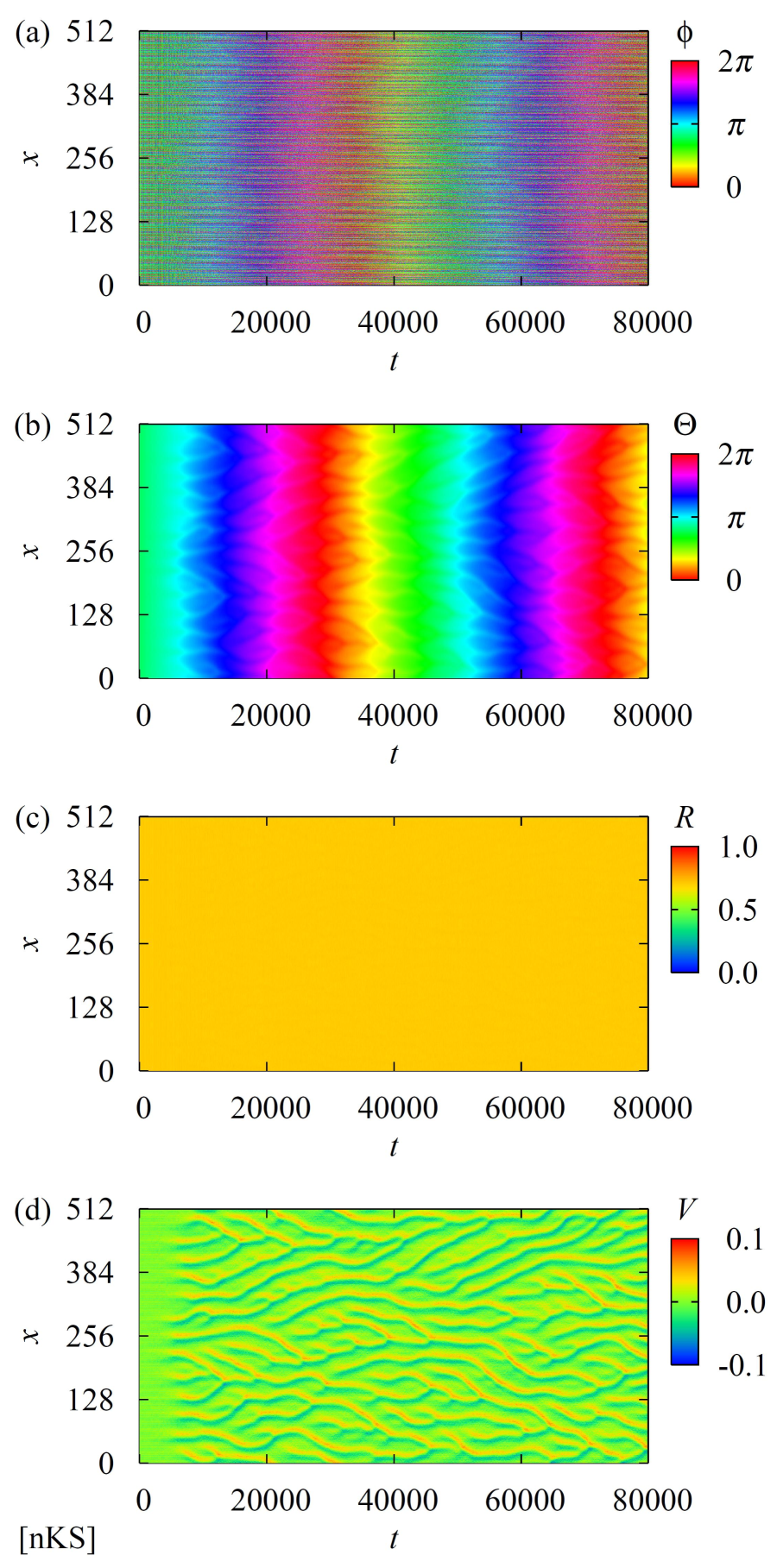
Figure 2: (color online). Numerical simulation of the nonlocal Kuramoto-Sakaguchi (nKS) model. The number of grid points is $2^{19}$. (a) Local phase $\phi(x,t)$. (b) Order parameter phase $\Theta(x,t)$. (c) Order parameter modulus $R(x,t)$. (d) Order parameter phase gradient $V(x,t)$.

Figure 3: (color online). Numerical simulation of the nonlocal Ott-Antonsen (nOA) equation. The number of grid points is $2^{11}$. (a) Local variable argument $\arg z(x,t)$. (b) Order parameter phase $\Theta(x,t)=\arg A(x,t)$. (c) Order parameter modulus $R(x,t)=|A(x,t)|$. (d) Order parameter phase gradient $V(x,t)=2\partial_{x}\Theta(x,t)$.

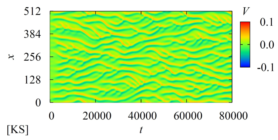
Figure 4: (color online). Numerical simulation of the Kuramoto-Sivashinsky (KS) equation. The number of grid points is $2^{11}$.

- (1) A. T. Winfree, The Geometry of Biological Time (Springer, Second Edition, New York, 2001).
- (2) Y. Kuramoto, Chemical Oscillations, Waves, and Turbulence (Springer, New York, 1984).
- (3) A. Pikovsky, M. Rosenblum, and J. Kurths, Synchronization: A Universal Concept in Nonlinear Sciences (Cambridge University Press, Cambridge, 2001).
- (4) Y. Kuramoto, in International Symposium on Mathematical Problems in Theoretical Physics, edited by H. Araki, Lecture Notes in Physics, Vol. 39 (Springer, New York, 1975), p. 420.
- (5) H. Sakaguchi and Y. Kuramoto, Prog. Theor. Phys. 76, 576 (1986).
- (6) Y. Kuramoto and D. Battogtokh, Nonlinear Phenom. Complex Syst. 5, 380 (2002).
- (7) S. H. Strogatz, Physica D 143, 1 (2000).
- (8) J. A. Acebrón, L. L. Bonilla, C. J. Pérez Vicente, F. Ritort, and R. Spigler, Rev. Mod. Phys. 77, 137 (2005).
- (9) A. Arenas, A. Díaz-Guilera, J. Kurths, Y. Moreno, and C. Zhou, Phys. Rep. 469, 93 (2008).
- (10) I. Z. Kiss, Y. Zhai, and J. L. Hudson, Science 296, 1676 (2002).
- (11) I. Z. Kiss, C. G. Rusin, H. Kori, and J. L. Hudson, Science 316, 1886 (2007).
- (12) A. F. Taylor, M. R. Tinsley, F. Wang, Z. Huang, and K. Showalter, Science 323, 614 (2009).
- (13) M. R. Tinsley, S. Nkomo, and K. Showalter, Nature Physics 8, 662 (2012).
- (14) S. Nkomo, M. R. Tinsley, and K. Showalter, Phys. Rev. Lett. 110, 244102 (2013).
- (15) Y. Kuramoto and T. Tsuzuki, Prog. Theor. Phys. 52, 1399 (1974).
- (16) Y. Kuramoto and T. Tsuzuki, Prog. Theor. Phys. 55, 356 (1976).
- (17) M. C. Cross and P. C. Hohenberg, Rev. Mod. Phys. 65, 851 (1993).
- (18) I. S. Aranson and L. Kramer, Rev. Mod. Phys. 74, 99 (2002).
- (19) M. Kim, M. Bertram, M. Pollmann, A. von Oertzen, A. S. Mikhailov, H. H. Rotermund, and G. Ertl, Science 292, 1357 (2001).
- (20) A. S. Mikhailov and K. Showalter, Phys. Rep. 425, 79 (2006).
- (21) A. S. Mikhailov and G. Ertl (Editors), Engineering of Chemical Complexity (World Scientific, Singapore, 2013).
- (22) G. I. Sivashinsky, Acta Astronautica 4, 1177 (1977).
- (23) Y. Kuramoto, Prog. Theor. Phys. 63, 1885 (1980).
- (24) Y. Kuramoto, Prog. Theor. Phys. 71, 1182 (1984).
- (25) E. Ott and T. M. Antonsen, Chaos 18, 037113 (2008).
- (26) E. Ott and T. M. Antonsen, Chaos 19, 023117 (2009).
- (27) C. R. Laing, Physica D 238, 1569 (2009).
- (28) C. R. Laing, Physica D 240, 1960 (2011).
- (29) W. S. Lee, J. G. Restrepo, E. Ott, and T. M. Antonsen, Chaos 21, 023122 (2011).
- (30) G. Bordyugov, A. Pikovsky, and M. Rosenblum, Phys. Rev. E 82, 035205(R) (2010).
- (31) M. Wolfrum, O. E. Omel’chenko, S. Yanchuk, and Y. L. Maistrenko, Chaos 21, 013112 (2011).
- (32) O. E. Omel’chenko, Nonlinearity 26, 2469 (2013).
- (33) Y. Kawamura, H. Nakao, and Y. Kuramoto, Phys. Rev. E 75, 036209 (2007). [arXiv:nlin/0702042]
- (34) Y. Kawamura, H. Nakao, K. Arai, H. Kori, and Y. Kuramoto, Chaos 20, 043109 (2010). [arXiv:1007.4382]
- (35) Y. Kawamura, H. Nakao, K. Arai, H. Kori, and Y. Kuramoto, Chaos 20, 043110 (2010). [arXiv:1007.5161]