Inference for Monotone Functions Under Short and Long Range Dependence: Confidence Intervals and New Universal Limits

Abstract

We introduce new point-wise confidence interval estimates for monotone functions observed with additive, dependent noise. Our methodology applies to both short- and long-range dependence regimes for the errors. The interval estimates are obtained via the method of inversion of certain discrepancy statistics. This approach avoids the estimation of nuisance parameters such as the derivative of the unknown function, which previous methods are forced to deal with. The resulting estimates are therefore more accurate, stable, and widely applicable in practice under minimal assumptions on the trend and error structure. The dependence of the errors especially long-range dependence leads to new phenomena, where new universal limits based on convex minorant functionals of drifted fractional Brownian motion emerge. Some extensions to uniform confidence bands are also developed.

Keywords. Isotonic Regression, Trend Estimation, Weak Dependence, Strong Dependence.

1 Introduction

The estimation of a trend function observed with additive noise is a canonical problem of substantial interest, widely studied in the statistical literature (see e.g. Clifford et. al.(2005)[9], Fan and Yao (2003)[11], Robinson (2009)[35], Wu and Zhao (2007) [46]). Most existing methods are based upon smoothness conditions on the trend (e.g. higher order differentiability, or curvature). They do not incorporate shape constraints like monotonicity or convexity, even in the presence of such information. Monotonicity, in particular, is naturally associated with trend functions arising in many disciplines like climatology (e.g. global warming), environmental and air pollution (e.g. ground-level Ozone or fine particulate matter (PM₁₀ or PM_2.5) as a function of temperature or humidity), engineering (diurnal trends in network traffic loads), among many others. One motivating application, illustrated in Figures 3 and 4 below, involves the annual global temperature anomalies data available at the NASA website [27]. The data comprises annual temperature records, measured relative to a baseline mean temperature, during the period 1850–1999; see also Jones and Mann (2002)[20] for a study of the paleoclimatic temperature and Steig et. al. (2009)[38] for evidence of warming trends at Antarctic locations. In the context of environmental pollution, monotone trends have been observed, for example, in the monitoring of water quality (Meal, 2001[22]), and mercury concentration of edible fish (Hussian et. al. 2005 [18]). In air pollution monitoring it is often the case that important factors (temperature, humidity, elevation) have an isotonic effect on the concentration of pollutants[26]. In many such scenarios, a natural model for the response as a function of time (or another natural covariate) is to write it as in (1) as the sum of an unobserved monotone trend function and dependent noise. A fundamental problem of interest is then to provide accurate confidence intervals for the underlying parameter that work well in practice under a variety of trend and dependence conditions on the data. It is desirable, for purposes of improved inference, to let the monotonicity constraint inform the statistical analysis of the data.

In the context of independent observations, the study of isotonic inference dates back to Rao (1969)[31]. Since then, the field has amassed a large body of research (see e.g. Banerjee and Wellner (2001, 2005)[4, 5], Banerjee (2007,2009) [6, 7], Brunk (1970) [8], Groeneboom (1985) [13], Groeneboom and Wellner (1992) [15], Woodroofe and Sun (1993) [44], Sun and Woodroofe (1996) [40], to name a few). Yet, isotonic inference in the presence of dependence is relatively less developed, despite a clear need for it. Recent breakthrough was achieved thanks to the important work of Anevski and Hossjer (2006) [2] (henceforth AH) and Zhao and Woodroofe (2012)[47] (subsequently ZW). AH develops a general asymptotic scheme for inference under order restrictions that applies, in principle, to arbitrary dependence in the model. A number of practical, as well as, theoretical challenges, however, remain open. Most notably, deriving confidence intervals (based on the work AH and ZW) requires estimation of the derivative $m^{\prime}(t_{0})$ of the unknown function. This is known to be a difficult problem in the context of shape restricted inference and often leads to biased confidence intervals and substantial under-coverage in practice, as will be demonstrated later.

This paper develops new methodology (and the corresponding theory), purely within the isotonic regression framework, in the signal plus noise model for making inference on a monotone trend function that largely circumvents the nuisance parameter estimation problems above and is substantially more robust to functions ill-behaved around the point of interest. Our approach should be contrasted with ones that combine isotonization with smoothing; see, for example Mammen (1991) [21], Mukherjee (1988) [25], Pal and Woodroofe (2007) [28], Ramsay (1998) [30] where a variety of methods of this type have been developed in the i.i.d. framework, but typically under higher order smoothness assumptions. Here, our goal is to work under minimal smoothness assumptions and to provide estimates that apply to a broad variety of both weakly and strongly dependent (stationary) error structures.

In Section 5, we describe a general methodology for constructing point-wise confidence intervals in both short- and long-range dependence settings. The supporting theory is presented in Section 4. The performance of this methodology is studied with extensive simulations and shown to generally outperform existing estimates in terms of both coverage accuracy and length of the resulting intervals. Most notably, we offer a new type of dependence-adaptive procedure, which works under both weak and strong dependence in the data requiring minimal assumptions on the trend and dependence structure. We also extend our point-wise methodology to construct conservative confidence bands under short-range dependence. Section 6 contains details of the simulation studies as well as applications of our methods to two real data problems where monotonicity constraints as well as dependence are natural and ubiquitous.

2 Problem formulation and overview of the results

Consider the isotonic regression model

$$Y_{i}=m(t_{i})+\epsilon_{i},\ \ i=1,\cdots,n,$$ (1)

where $m:[0,1]\to{\mathbb{R}}$ is an unknown monotone non-decreasing function, $t_{i}=i/n,\ i=1,\cdots,n$ is a fixed uniform design and where the errors $\epsilon_{i}$ have zero means and variance ${\rm Var}(\epsilon_{i})=\sigma^{2}.$ We are interested in the case where the noise is dependent. We shall model it by a stationary time series $\{\epsilon_{k}\}_{k\in\mathbb{Z}}$, which may have either weak or strong dependence (cf Section 3, below). The trend $m$ will be assumed monotone non-decreasing and to satisfy the following mild condition.

Assumption C. The regression function $m(t)$ is continuously differentiable in a neighborhood of $t_{0}$ with $m^{\prime}(t_{0})>0$.

Our ultimate goal is to construct an asymptotic confidence interval for $m(t_{0})$, $(0<t_{0}<1)$, which is largely robust to the dependence structure of the errors. To this end, we consider the testing problem: $H_{0}:m(t_{0})=\theta_{0}$ vs. $H_{1}:m(t_{0})\neq\theta_{0}$. Confidence intervals for $m(t_{0})$ will be obtained by inversion of acceptance regions of tests for the above problem. Consider the usual isotonic regression estimate (IRE) of $m$ (cf. Robertson et. al. (1988)[34]), obtained as

$$(\hat{m}_{n}(t_{i}),\ i=1,\cdots,n)=\mathop{\rm Argmin}_{m_{1}\leq\cdots\leq m_{n}}\sum_{i=1}^{n}(Y_{i}-m_{i})^{2}.$$ (2)

To address the above testing problem, we also consider the following constrained isotonic estimate $\hat{m}_{n}^{0}$. Let $l=\lfloor nt_{0}\rfloor$, so that $t_{l}\leq t_{0}<t_{l+1}$ and define

$$(\hat{m}_{n}^{0}(t_{i}),\ i=1,\cdots,n)=\mathop{\rm Argmin}_{m_{1}\leq\cdots\leq m_{l}\leq\theta_{0}\leq m_{l+1}\leq\cdots\leq m_{n}}\sum_{i=1}^{n}(Y_{i}-m_{i})^{2}.$$ (3)

Note that both functions $\hat{m}_{n}$ and $\hat{m}_{n}^{0}$ are identified only at the grid points. By convention, we extend them as left-continuous piece-wise constant functions defined on the entire interval $(0,1]$.

Our hypothesis tests will be based on the following discrepancy statistics

$$L_{n} =\frac{n}{\sigma_{n}^{2}}\left(\sum_{i=1}^{n}(Y_{i}-\hat{m}_{n}^{0}(t_{i}))^{2}-\sum_{i=1}^{n}(Y_{i}-\hat{m}_{n}(t_{i}))^{2}\right)\equiv\frac{n}{\sigma_{n}^{2}}\,\mathbb{L}_{n}$$ (4)

$$T_{n} =\frac{n}{\sigma_{n}^{2}}\sum_{i=1}^{n}\left(\hat{m}_{n}(t_{i})-\hat{m}_{n}^{0}(t_{i})\right)^{2}\equiv\frac{n}{\sigma_{n}^{2}}\,\mathbb{T}_{n},$$

where $\sigma_{n}^{2}={\rm Var}(\sum_{k=1}^{n}\epsilon_{k})$. A third statistic which will prove particularly useful in the long-range dependence case is the ‘ratio statistic’ $R_{n}:=L_{n}/T_{n}$. Its asymptotic properties will be derived from the joint asymptotic behavior of $L_{n}$ and $T_{n}$.

In the rest of this section, we give the intuition behind our methodology. The precise asymptotic results are given in Section 4. Consider the rescaled discrepancy statistics $\mathbb{L}_{n}$ and $\mathbb{T}_{n}$ in (4). As shown in Banerjee (2009)[7], in the i.i.d. setting if $m(t_{0})=\theta_{0}$, then $\mathbb{L}_{n}/\sigma^{2}\Rightarrow{\mathbb{L}}$, where ${\mathbb{L}}$ is a positive random variable expressed as a functional of the two-sided Brownian motion plus quadratic drift $\{\mathbb{W}(t)+t^{2}\}_{t\in{\mathbb{R}}}$ and $\sigma^{2}$ is the common variance of the errors. Further, the closely related $L^{2}$-type discrepancy statistic $\mathbb{T}_{n}$ is similarly shown to satisfy: $\mathbb{T}_{n}/\sigma^{2}\Rightarrow{\mathbb{T}}$, where the limit ${\mathbb{T}}$ is another functional of $\{\mathbb{W}(t)+t^{2}\}_{t\in{\mathbb{R}}}$. As both these limits are universal (free of the parameters of the problem), the confidence sets obtained by the method of inversion of these statistics do not involve the nuisance parameter $m^{\prime}(t_{0})$ – a most challenging quantity to estimate in practice. Only an estimate of $\sigma^{2}$ is required, which easy to obtain in practice. This methodology in the i.i.d. setting has lead to accurate confidence intervals, which work well in practice for rather challenging isotonic trends. The asymptotic phenomena encountered in the i.i.d. case then naturally motivate us to investigate whether similar benefits accrue from the above statistics in the dependent case.

In the case of dependent errors two fundamentally different regimes arise: (i) short-range dependence and (ii) long-range dependence. The finite variance stationary time series in (1) is said to be long-range dependent if $\sum_{k=1}^{\infty}|{\rm Cov}(\epsilon_{k},\epsilon_{0})|=\infty$ and if the latter covariances are summable, it is referred to as short-range dependent (see e.g. Doukhan et. al. (2003) [10]). We refer to $\mbox{Cov}(\epsilon_{k},\epsilon_{0})$ as $\mbox{Cov}(k)$, the covariance at lag $k$ which is well-defined by stationarity.

In the short-range dependence context, one expects that the discrepancy statistics $\mathbb{L}_{n}$ and $\mathbb{T}_{n}$ will have similar asymptotic behavior to the independent errors situation. We show in Theorem 4.1 below that, under mild assumptions, this is indeed the case, and in fact, under $m(t_{0})=\theta_{0}$, we have the following joint convergence:

$$(\mathbb{L}_{n}(\theta_{0})/\tau^{2},\mathbb{T}_{n}(\theta_{0})/\tau^{2})\Longrightarrow({\mathbb{L}},{\mathbb{T}}),\ \ \mbox{ as }n\to\infty,$$

where $\tau^{2}=\sum_{k=-\infty}^{\infty}{\rm Cov}(k)$ and ${\mathbb{L}}$ and ${\mathbb{T}}$ are functionals of the same quadratically drifted standard Brownian motion. In practice, this result justifies an effective and robust inference methodology for constructing confidence intervals for $m(t_{0})$ via the method of inversion (Section 5.2), where the only parameter that needs to be estimated is $\tau^{2}$.

In the long-range dependence setting, the discrepancy statistics $\mathbb{L}_{n}$ and $\mathbb{T}_{n}$ exhibit fundamentally new behavior. In fact, the problem here is ill-posed since multiple different types of long-range dependence may arise (Samorodnitsky, 2006) [37]. In this paper, we focus on one of the most frequently encountered long-range dependence regimes where the cumulative sums of the error sequence converge to the fractional Brownian motion (fBm, in short): see Section 3. In this setting, from Theorem 4.2 below, we get that

$$r_{n}\,(\mathbb{L}_{n}(\theta_{0}),\mathbb{T}_{n}(\theta_{0}))\Longrightarrow C\,(\mathbb{L}^{(H)},\mathbb{T}^{(H)}),$$

where the factor $r_{n}$ and the constant $C$ are both unknown and the limits $\mathbb{L}^{(H)}$ and $\mathbb{T}^{(H)}$ are now expressed as functionals of a standard two-sided fBm plus quadratic drift $\{B_{H}(t)+t^{2}\}_{t\in{\mathbb{R}}}$. The functionals defining $\mathbb{L}^{(H)}$ and $\mathbb{T}^{(H)}$ are similar to those defining $\mathbb{L}$ and $\mathbb{T}$, respectively. Their analysis, however, requires new results on the behavior of greatest convex minorants of fBm plus quadratic drift, which may be of independent interest (see Supplement B). The distributions of $\mathbb{L}^{(H)}$ and $\mathbb{T}^{(H)}$ only depend on the Hurst parameter $H\in(1/2,1)$ of the fractional Brownian motion.

In contrast to the weak dependence case, inversion of the $\mathbb{L}_{n}$ or $\mathbb{T}_{n}$ statistics to construct confidence intervals in the long-range dependence case requires the estimation of $m^{\prime}(t_{0})$, since the constant $C$ depends on it. One can eliminate this nuisance parameter, however, by considering the ratio statistic $R_{n}:=\mathbb{L}_{n}/\mathbb{T}_{n}$. This can be thought of as a self-normalization. We show that the limit distribution of $R_{n}$ depends only on the Hurst parameter $H$ (Theorem 5.1). This result, again through the method of inversion, yields confidence intervals for $m(t_{0})$ without having to estimate the derivative. In practice, $H$ is the only parameter that needs to be estimated, but this problem has received considerable attention in the literature (see e.g. Fay et. al. (2009)[12] and references therein). Our confidence intervals based on plug-in estimates of $H$ have close to nominal coverage (cf Table 6 in Supplement A). In fact, a certain partial nesting property of the quantiles of the asymptotic distribution can be used to obtain conservative confidence intervals without having to estimate $H$ precisely (see, Section 6, below for more detials). Furthermore, the new ratio statistic can also be used in the short-range dependence and, in particular, the i.i.d. context ($H=1/2$). It provides an alternative methodology to that based on the discrepancy statistics $\mathbb{L}_{n}$ and $\mathbb{T}_{n}$, where in fact no estimation of $\tau^{2}$ is necessary!

Selected quantiles of this new family of universal limit distributions are tabulated in the short- and long-range dependence regimes (Table 1 in the paper and Tables 1 through 4 in Supplement B). A striking feature of these quantiles, discussed in detail in Section 6.1, is a type of partial nesting as a function of $H$. It allows one to obtain conservative intervals with 90% or 95% nominal coverage from the ratio statistic without a precise estimate of $H$, provided the true value of $H$ is not very close to 1. Thus, inference based on the ratio statistic provides a remarkable degree of robustness across both short and long-range dependence.

3 Dependence structure

In this section, we introduce and discuss our formal assumptions on the dependence structure of the errors $\epsilon_{i}$’s in (1). These assumptions will be tacitly adopted for the rest of the paper and will require some technicalities for a precise description.

We suppose that the errors have zero means, finite variances and form a strictly stationary time series $\{\epsilon_{k}\}_{k\in{\mathbb{Z}}}$. Let $S_{n}=\sum_{k=1}^{n}\epsilon_{k},$ and consider the piece-wise linear cumulative sum diagram

$$w_{n}(t)=\frac{1}{\sigma_{n}}{\Big{(}}\sum_{i=1}^{\lfloor nt\rfloor}\epsilon_{i}+(nt-\lfloor nt\rfloor)\epsilon_{\lfloor nt\rfloor+1}{\Big{)}},\quad\mbox{ where }\quad\sigma_{n}^{2}={\rm Var}(S_{n}).$$ (5)

The asymptotic behavior of the process $\{w_{n}(t)\}_{t\geq 0}$ is generally determined by the degree of dependence of the errors in addition to their tail behavior. If the $\epsilon_{i}$’s are weakly dependent, then as in the usual Donsker theorem, the limit is the Brownian motion and the corresponding statistical results are similar to the situation of independent errors. On the other hand, as noted in the introduction, strong dependence of the $\epsilon_{i}$’s leads to different types of limits and new statistical theory. We shall consider two different regimes: [i] short-range dependent errors, and, [ii] long-range dependent errors, as explained in Section II.

3.0.1 Short-range dependence

To formalize weak dependence, let $\|\cdot\|$ denote the $L^{2}$ norm on the probability space and introduce the discrete filtration ${\cal F}_{n}=\sigma\{\epsilon_{m},\ m\leq n\},\ n\in{\mathbb{Z}}$, i.e. ${\cal F}_{n}$ is the $\sigma$-algebra generated by all errors up to and including ‘time’ $n$. In the short-range dependent case, following ZW[47], we assume that

$$\sum_{n=1}^{\infty}n^{-\frac{3}{2}}\|\mathbb{E}(S_{n}|\mathcal{F}_{0})\|<\infty.$$ (6)

It is shown in Peligrad and Utev (2005)[29] that if (6) is satisfied then,

$$\Gamma:=\sum_{k=0}^{\infty}2^{-\frac{1}{2}k}\|\mathbb{E}(S_{2^{k}}|\mathcal{F}_{0})\|<\infty\quad\mbox{ {\em and} }\quad\mathbb{E}\left[\max_{k\leq n}S_{k}^{2}\right]\leq 6\left[\mathbb{E}(\epsilon_{1}^{2})+\Gamma\right]n.$$ (7)

Furthermore, the limit

$$\tau^{2}=\lim_{n\to\infty}\frac{1}{n}\mathbb{E}(S_{n}^{2})<\infty$$ (8)

exists and the process $\{w_{n}(t)\}_{0\leq t\leq 1}$ converges in distribution to the Brownian motion $\mathbb{B}$ in the space $D[0,1]$ equipped with the usual $J_{1}$-Skorohod topology.

Remark 3.1.

In AH[2], weak dependence was quantified in terms of mixing conditions. Here, we use an alternative condition (6) from ZW[47], implied by the strong mixing Assumption (A9) of AH[2], and therefore weaker.

3.0.2 Long-range dependence

A great variety of models exhibit long-range dependence. We focus here on a special but important case when the error $\epsilon_{k}=g(\xi_{k}),\ k\in\mathbb{Z}$, where $\left\{\xi_{i}\right\}_{i\in\mathbb{Z}}$ is a stationary Gaussian time series with zero mean. The function $g$ is deterministic and from $L^{2}(\phi)$ where $\phi$ denotes standard normal density, i.e., $\mathbb{E}(g(Z))^{2}=E(\epsilon_{1}^{2})<\infty$ where $Z\sim N(0,1)$ . In this setting, an elegant theory characterizing the possible limits of the cumulative sums in (5) was developed in the seminal work of Taqqu (1975[41], 1979[42]).

Following AH[2], let ${\rm Cov}(k)=\mathbb{E}(\xi_{i}\xi_{i+k})$ be such that ${\rm Cov}(0)=1$ and ${\rm Cov}(k)=k^{-d}l_{0}(k)$, where $0<d<1$ is fixed and $l_{0}$ is a function slowly varying at infinity, i.e., for all $a>0$, $l_{0}(ax)/l_{0}(x)\to 1$, as $x\to\infty$.

As $\mathbb{E}(g(Z)^{2})<\infty$, the function $g$ can be expanded using Hermite polynomials and we have the representation:

$$\epsilon_{i}:=g(\xi_{i})=\sum_{k=r}^{\infty}\frac{\eta_{k}}{k!}H_{k}(\xi_{i}),$$

where the series converges in $L^{2}(\mathbb{P})$, $\eta_{k}=\mathbb{E}(g(\xi_{i})H_{k}(\xi_{i})),\ k\geq r$; the $H_{k}$’s are the Hermite polynomials of order $k$ and the summation starts from $r\geq 1$ – the index of the first nonzero coefficient in the expansion. Note that $r\geq 1$ corresponds to centered $\epsilon_{i}$’s, since $E(H_{k}(\xi_{1}))=0$ for all $k\geq 1$. The index $r$ is referred to as the Hermite rank of the function $g$. For the rest of the paper we restrict our discussion to the case $r=1$

The results of Taqqu (1975[41], 1979[42]) show that if $0<d<1$, the sequence $\{\epsilon_{i}\}$ also exhibits long-range dependence and, in fact,

$${\Big{\{}}\sigma_{n}^{-1}w_{n}(t){\Big{\}}}_{t\in[0,1]}\Longrightarrow{\Big{\{}}B_{H}(t){\Big{\}}}_{t\in[0,1]},$$ (9)

in $D[0,1]$ equipped with Skorohod topology, where the limit process $B_{H}$ is a Gaussian process in $C[0,1]$ a.s. with stationary increments. It can be shown that

$$\sigma_{n}^{2}=\eta_{1}^{2}n^{2-d}l_{1}(n)(1+o(1)),$$ (10)

where $l_{1}$ is another slowly varying function: $l_{1}(k)={2l_{0}(k)}/(1-d)(2-d))$. The process $B_{H}$ can be uniquely extended to a process on the entire line with stationary increments which is denoted by the same symbol and known as the fractional Brownian motion (fBm) with self-similarity parameter (also called Hurst index) $H=1-d/2$: i.e. for all $c>0$, the processes $\{B_{H}(ct)\}_{t\in\mathbb{R}}$ and $\{c^{H}B_{H}(t)\}_{t\in\mathbb{R}}$ are equal in distribution. The stationarity of the increments and self-similarity imply that

$${\rm Cov}(B_{H}(t),B_{H}(s))=\frac{\sigma^{2}}{2}{\Big{(}}|t|^{2H}+|s|^{2H}-|t-s|^{2H}{\Big{)}},\ \ t,s\in\mathbb{R}.$$ (11)

For more details on the properties of the fBm, see e.g. the review chapter by Taqqu in Doukhan et. al. (2003)[10].

4 Key results

We present in this section the joint asymptotic behavior of the statistics $L_{n}$ and $T_{n}$ which is central to the subsequent methodology. To this end, we first introduce the greatest convex minorant (GCM) functional.

Greatest convex minorants: Let $\mathcal{T}_{I}(f)$ denote the GCM of a real-valued function $f$, defined on an interval $I\subseteq\mathbb{R}$. For an interval $J\subset I$, we denote the GCM of the restriction of $f$ to $J$ by $\mathcal{T}_{J}(f)$. When $f$ is defined on $\mathbb{R}$, we sometimes write $\mathcal{T}(f)$ for $\mathcal{T}_{\mathbb{R}}(f)$ and $\mathcal{T}_{c}(f)$ for $\mathcal{T}_{[-c,c]}(f)$. Also, let $\mathcal{L}(f)$ denote the left derivative functional of a convex function $f$, which is a well-defined, non-decreasing and left-continuous function (cf. Theorem 24.1 of Rockafellar (1970)[36]).

Define the process: $\{\mathbb{G}(z)\}_{z\in\mathbb{R}}\equiv\{\mathbb{G}_{a,b}(z)\}_{z\in\mathbb{R}}:=\{a\mathbb{W}(z)+bz^{2}\}_{z\in\mathbb{R}}$, where $b=\frac{1}{2}m^{\prime}(t_{0})$ and (i) (under weak dependence) $\mathbb{W}$ is a two-sided Brownian motion on $\mathbb{R}$, and $a:=\tau$ given in (8), (ii) (under strong dependence) $\mathbb{W}$ is the fBm process $B_{H}$ and $a:=|\eta_{1}|$.
Next, define the following slope-of-greatest-convex-minorant functionals as follows:

$$\mathcal{S}_{a,b}(z) = \mathcal{L}\circ\mathcal{T}\left(\mathbb{G}\right)(z)$$ (12)

$$\mathcal{S}_{a,b}^{h}(z) = \left\{\begin{array}[]{lll}\mathcal{L}\circ\mathcal{T}_{(-\infty,0)}\left(\mathbb{G}\right)(z)\wedge h&,\ z\in(-\infty,0)\\ \lim_{u\uparrow 0}\mathcal{L}\circ\mathcal{T}_{(-\infty,0)}\left(\mathbb{G}\right)(u)\wedge h&,\ z=0\\ \mathcal{L}\circ\mathcal{T}_{(0,\infty)}\left(\mathbb{G}\right)(z)\vee h&,\ z\in(0,\infty)\\ \end{array}\right.$$ (16)

We are now ready to state the limit distributions of the statistics $L_{n}$ and $T_{n}$ in terms of $\mathcal{S}_{a,b}(z)$ and $\mathcal{S}_{a,b}^{0}(z)$. Define:

$$\mathbb{L}_{a,b}=\int_{\mathbb{R}}\Big{(}(\mathcal{S}_{a,b}(z))^{2}-(\mathcal{S}_{a,b}^{0}(z))^{2}\Big{)}dz\ \mbox{ and }\ \mathbb{T}_{a,b}=\int_{\mathbb{R}}\left(\mathcal{S}_{a,b}(z)-\mathcal{S}_{a,b}^{0}(z)\right)^{2}dz.$$ (17)

Remark 4.1.

The processes $\mathcal{S}_{a,b}(z)$ and $\mathcal{S}_{a,b}^{0}(z)$ differ on a compact interval. This is rigorously established in Theorem 3.1 of Supplement B showing that the statistics in (17) are proper random variables.

Remark 4.2.

In the long-range dependence case where $\mathbb{L}_{a,b}$ and $\mathbb{T}_{a,b}$ depend on the Hurst index $H$, we denote them by $\mathbb{L}_{a,b}^{(H)}$ and $\mathbb{T}_{a,b}^{(H)}$. When $a=b=1$, we drop the subscripts and write $\mathbb{L}$ and $\mathbb{T}$ in the short-range dependence case, and $\mathbb{L}^{(H)}$ and $\mathbb{T}^{(H)}$ in the long-range dependence case. In the following sections we will, often, drop $H$ and just use $\mathbb{L}$ and $\mathbb{T}$ for both short- and long-range dependence when there is no chance of confusion.

Theorem 4.1.

For short-range dependent errors, $(L_{n},T_{n})\Rightarrow(\mathbb{L},\mathbb{T})$, as $n\to\infty$.

Remark 4.3.

Since $\sigma_{n}^{2}\sim n\,\tau^{2}$ under short-range dependence, the above result can be rewritten as:

$$\frac{1}{\tau^{2}}\,(\mathbb{L}_{n},\mathbb{T}_{n})\Rightarrow(\mathbb{L},\mathbb{T}),as\;n\to\infty.$$ (18)

Theorem 4.2.

For long-range dependent errors, as $n\to\infty$,

$$\frac{\sigma_{n}^{2}}{n^{2}d_{n}^{3}}(L_{n},T_{n})\Longrightarrow a^{2}\left(\frac{a}{b}\right)^{\frac{2H-1}{2-H}}(\mathbb{L}^{(H)},\mathbb{T}^{(H)}),$$ (19)

where $a=|\eta_{1}|,b=\frac{1}{2}m^{\prime}(t_{0})$, $\sigma_{n}^{2}$ is as defined at the beginning of Section III and $d_{n}\rightarrow 0$ is as in Theorem A.1 (ii).

The proof in the long-range dependent case is given in Appendix B. The proof in the simpler, short-range case is similar and omitted for brevity. For a proof-sketch of the asymptotics of $L_{n}$ and $T_{n}$ see Appendix A.

Remark 4.4.

Using the definitions of $L_{n},T_{n}$ in (4), the result of Theorem 4.2 can be restated as:

$$\frac{1}{n\,d_{n}^{3}}(\mathbb{L}_{n},\mathbb{T}_{n})\Longrightarrow a^{2}\left(\frac{a}{b}\right)^{\frac{2H-1}{2-H}}(\mathbb{L}^{(H)},\mathbb{T}^{(H)})\,.$$ (20)

Now, by Theorem A.1 (ii), $d_{n}=n^{-d/(2+d)}\,l_{2}(n)$ where $d$ is the long memory parameter encountered in Section III.2 and $l_{2}(n)$ is a slowly varying function related to $l_{1}(n)$ that appears in the representation of $\sigma_{n}^{2}$ in (10). The long-range dependent error structures generally used in statistical applications, and, in particular, in our paper – namely, Fractional Gaussian Noise (FGN) and FARIMA processes – have trivial slowly varying functions: $l_{1}(n)=1$ and (therefore) $l_{2}(n)=1$, and in such cases the above display further simplifies to:

$$\frac{1}{n^{1-3d/(2+d)}}(\mathbb{L}_{n},\mathbb{T}_{n}) = n^{-(2H-1)/(2-H)}(\mathbb{L}_{n},\mathbb{T}_{n})$$ (21)

$$\Longrightarrow a^{2}\left(\frac{a}{b}\right)^{\frac{2H-1}{2-H}}(\mathbb{L}^{(H)},\mathbb{T}^{(H)})\,,$$ (22)

using $H=1-d/2$.

5 Methodology

5.1 An asymptotically pivotal ratio statistic

Recall (18). To be able to use the statistics $\mathbb{L}_{n},\mathbb{T}_{n}$, one needs a suitable ‘plug-in’ estimate for $\tau^{2}$ in (8), but this can typically be estimated well in practice. The use of the statistics $\mathbb{L}_{n}$ and $\mathbb{T}_{n}$ in the LRD case, however, is more problematic because by (21), the limit distributions involve the derivative $m^{\prime}(t_{0})$ (appearing in the constant $b$) which is difficult to estimate, and in addition, the quantities $\eta_{1}$ (appearing in the constant $a$) and $H$ (both in the normalization of the test statistics and the limit distributions). An elegant way to eliminate the need for estimating $m^{\prime}(t_{0})$ as well as $\eta$ and the $H$-dependent normalization on the right side of (21) is to consider the ratio statistic, introduced next.

Note that $L_{n}$ and $T_{n}$ are always non-negative by definition. By (4), if $T_{n}=0$ we have $L_{n}=0$. Also, as shown in Lemma 3.1 from Supplement A, we have $L_{n}\geq T_{n}$. Therefore $L_{n}$ and $T_{n}$ are either both equal to $0$ or both strictly positive. Similarly (17) implies that if $\mathbb{T}=0$, then $\mathbb{L}=0$ and by Theorems 4.1 and 4.2 and the Portmanteau theorem, we obtain that $\mathbb{L}\geq\mathbb{T}$ almost surely. It follows again that $\mathbb{T}$ and $\mathbb{L}$ are also either both equal to $0$ or strictly positive.

Now, define the ratio statistic $R_{n}=L_{n}/T_{n}\equiv\mathbb{L}_{n}/\mathbb{T}_{n}$, where $0/0$ is interpreted as 1. By the discussion in the above paragraph, $\mathbb{P}(R_{n}<\infty)=1$.

Theorem 5.1.

For both short- and long-range dependent errors, we have

$$R_{n}\Longrightarrow\mathcal{R}:=\frac{\mathbb{L}}{\mathbb{T}},\ \quad\mbox{ as }n\to\infty,$$

where the limit has a proper probability distribution.

Proof.

The convergence follows from Theorems 4.1, 4.2 and the Continuous Mapping Theorem, provided that $\mathbb{P}(\mathbb{T}=0)=0$. The latter is true thanks to Theorem 3.2 in Supplement B. $\Box$ ∎

Remark 5.1.

Note that though the computation of $R_{n}$ does not require us to know/estimate $H$, the limit distribution of $R_{n}$ does involve the Hurst parameter.

5.2 Construction of Confidence Intervals

We first focus on the use of the statistics $\mathbb{L}_{n}$ and $\mathbb{T}_{n}$.
Short-range dependence: Let $\mathbb{L}_{n}(\theta)$ and $\mathbb{T}_{n}(\theta)$ denote the residual sum of squares and $L_{2}$ statistics, respectively, for testing $H_{0}:m(t_{0})=\theta$ against $H_{a}:m(t_{0})\neq\theta$. Letting $\theta_{0}$ denote the true value of $m(t_{0})$, an asymptotic level $1-\alpha$ confidence set for $\theta_{0}$, using inversion of $L_{n}$, is given by $\{\theta:\mathbb{L}_{n}(\theta)/\hat{\tau}^{2}\leq F_{\mathbb{L}}^{\leftarrow}(1-\alpha)\}$, where $F_{\mathbb{L}}^{\leftarrow}$ denotes the left-continuous quantile function of $F_{\mathbb{L}}$, the distribution function of ${\mathbb{L}}$ and $\hat{\tau}$ is a consistent estimate of $\tau$. For weakly dependent errors $\tau^{2}$ was estimated as

$$\hat{\tau}^{2}=\hat{\gamma}_{n}(0)+2\,\sum_{k\leq\sqrt{n}}\Big{(}1-\frac{k}{\sqrt{n}}\Big{)}\hat{\gamma}_{n}(k)$$ (23)

where $\hat{\gamma}_{n}(k)$ is the empirical auto-covariance of $\hat{e}_{i}:=Y_{i}-\hat{m}_{n}(t_{i})$ at lag $k$, i.e. $\hat{\gamma}_{n}(k)=n^{-1}\sum_{i=1}^{n-k}\,\hat{e}_{i}\,\hat{e}_{i+k}$. This is a consistent estimator under the presence of a monotone trend as shown in Theorem 2 of Wu et. al. (2001)[45].
The statistic $T_{n}$ can be used in an exact similar fashion to obtain confidence intervals.
By our results on the shape of $L_{n}(\theta)$ and $T_{n}(\theta)$ (which completely describe the shapes of $\mathbb{L}_{n}(\theta)$ and $\mathbb{T}_{n}(\theta)$) in Lemma 3.2 of Supplement A, letting,

$$C_{L}(\alpha):=\inf\{\theta:\mathbb{L}_{n}(\theta)/\hat{\tau}^{2}<F_{\mathbb{L}}^{\leftarrow}(1-\alpha)\}\hskip 7.22743pt\mbox{and}\hskip 7.22743ptC_{U}(\alpha):=\sup\{\theta:\mathbb{L}_{n}(\theta)/\hat{\tau}^{2}<F_{\mathbb{L}}^{\leftarrow}(1-\alpha)\}\,,$$

we conclude that $[C_{L}(\alpha),C_{U}(\alpha)]$ is precisely the set $\{\theta:L_{n}(\theta)\leq F_{\mathbb{L}}^{\leftarrow}(1-\alpha)\}$, giving us an asymptotic $100(1-\alpha)\%$ confidence interval for $\theta_{0}$. The lemma also ensures that the intervals produced by inverting $\mathbb{L}_{n}$ and $\mathbb{T}_{n}$ are always of finite length.

Long-range dependence: If $\hat{H}$ is a polynomial-rate-consistent estimate of $H$: i.e. $n^{\lambda}(\hat{H}-H)=O_{p}(1)$ for some $\lambda>0$, then

$$n^{-(2\hat{H}-1)/(2-\hat{H})}(\mathbb{L}_{n},\mathbb{T}_{n})\Longrightarrow a^{2}\left(\frac{a}{b}\right)^{\frac{2H-1}{2-H}}(\mathbb{L}^{(H)},\mathbb{T}^{(H)})\,.$$

The above result follows immediately from (21) and the fact that for a polynomial-rate-consistent $\hat{H}$, $n^{-(2\hat{H}-1)/(2-\hat{H})+(2H-1)/(2-H)}\rightarrow_{p}1$.
Furthermore, if $\hat{a},\hat{b}$ are consistent estimates of $a,b$ and $F_{\mathbb{L}^{(H)}}^{\leftarrow}(1-\alpha)$, the $(1-\alpha)$’th quantile of $\mathbb{L}^{(H)}$ is continuous in $H$, as suggested strongly by extensive simulations, $\{\theta:n^{-(2\hat{H}-1)/(2-\hat{H})}\mathbb{L}_{n}(\theta)\leq\hat{a}^{2}\,(\hat{a}/\hat{b})^{(2\,\hat{H}-1)/(2-\hat{H})}\,F_{\mathbb{L}^{(H)}}^{\leftarrow}(1-\alpha)\}$ gives an asymptotic level $1-\alpha$ confidence set for $\theta_{0}$, by an easy application of Slutsky’s lemma. As under short-range dependence, this is a confidence interval.
Details on the estimation of $H$ for our simulations and data analysis are provided later. Simulated quantiles for $\mathbb{L}$ for both short- and long-range dependent errors with different Hurst parameters $H$ are presented in Tables 3 and 4, Supplement B. In the sequel we will often refer to the $\mathbb{L}_{n}$ based intervals as $L_{n}$ based intervals.

We next turn to confidence sets using $R_{n}$ which avoids the estimation of difficult nuisance parameters in the long-range dependence case as discussed previously. Consider first, the shape of $R_{n}(\theta)$ as a function of $\theta$. It assumes the value $1$ at $\theta=\hat{m}_{n}(t_{0})$, converges to $1$ as $|\theta|\to\infty$ and displays irregular humps in between. Figure 1 illustrates the behavior of this statistic as a function of $h$, where $h=n^{1/3}(\theta-\theta_{0})$ under SRD and $h=d_{n}^{-1}(\theta-\theta_{0})$ under LRD. As a sensible inversion of $R_{n}$ should avoid values away from $\hat{m}_{n}(t_{0})$, an asymptotic confidence set should look like: $\{\theta:R_{n}(\theta)>\zeta\}$, where $\zeta>1$ is an appropriate quantile (depending on the level of confidence desired) of $\mathcal{R}$, the limiting random variable in Theorem 5.1. This will, however, not yield a confidence interval but a rather irregular confidence set, and, in particular, may miss values of $\theta$ close to $\theta_{0}$.

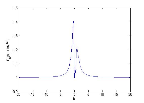
((a)) Short-range dependence

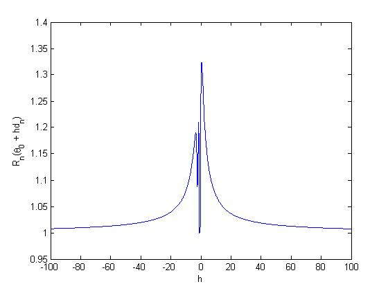
((b)) Long-range dependence

Figure 1: Shape of ratio statistic as a function of $h$

Another issue with using $R_{n}$ is that the quantiles of $\mathcal{R}$ grow extremely slowly from 1 and are hard to represent in a table. For matters of practical convenience, we therefore make a monotone transformation of $R_{n}$, namely,

$$\Psi_{n}(\theta)=\begin{cases}-\log(R_{n}(\theta)-1),&\mbox{if }R_{n}(\theta)>1\\ \infty,&\mbox{if }R_{n}(\theta)=1.\end{cases}$$

Then, the following Proposition follows easily from Theorem 5.1 and the Continuous Mapping Theorem.

Proposition 5.1.

Under the assumptions of Theorem 5.1, we have

$$\Psi_{n}(\theta_{0})\stackrel{{\scriptstyle d}}{{\to}}\Psi:=-\log(\mathcal{R}-1)\mbox{ as }n\to\infty.$$ (24)

where $\mathbb{P}(\Psi=\infty)=\mathbb{P}(\mathcal{R}=1)$.

As $\Psi_{n}$ is a monotone decreasing transformation of $R_{n}=L_{n}/T_{n}$, it exhibits the same irregularities; see Figure 1 in Supplement A, and therefore, in terms of $\Psi_{n}$, our confidence set $\{\theta:\Psi_{n}(\theta)<-\log(\zeta-1)\}$, is still irregular. To avoid this, we propose a confidence interval of the form $[\widetilde{C}_{L}(\alpha),\widetilde{C}_{u}(\alpha)]$, where $\widetilde{C}_{L}$ and $\widetilde{C}_{U}$ are defined thus:

$$\widetilde{C}_{L}(\alpha):=\inf\{\theta:\Psi_{n}(\theta)<F_{\Psi}^{\leftarrow}(1-\alpha)\},\;\;\widetilde{C}_{U}(\alpha):=\sup\{\theta:\Psi_{n}(\theta)<F_{\Psi}^{\leftarrow}(1-\alpha)\}.$$

Note that this gives us a conservative $100(1-\alpha)\%$ C.I. for $\theta_{0}$. Selected quantiles of $\Psi$ are presented in Table 1I. See, Supplement B, Tables 1 and 2 for a detailed presentation of the quantiles of $\Psi$.

While our knowledge of the behavior of $R_{n}(\theta)$ is limited, we do have the following result.

Proposition 5.2.

Let $\theta\neq\theta_{0}$ and $R_{n}(\theta)$ be the ratio statistic calculated under the null hypothesis $H_{0,\theta}:m(t_{0})=\theta$. Then, $R_{n}(\theta)\stackrel{{\scriptstyle P}}{{\to}}1$ as $n\to\infty$.

Equivalently, $\Psi_{n}(\theta)\stackrel{{\scriptstyle P}}{{\to}}\infty$, which means that the probability that any $\theta\neq\theta_{0}$ falls outside our proposed honest confidence interval converges to 1. The proof of this lemma is given in Section 3 of Supplement A (Proposition 3.2) which also contains additional discussions and speculations on the $\Psi_{n}(\theta)$ based confidence sets.

Table 1: Quantiles of $\Psi$

p	SRD	H = 0.7	H = 0.8	H = 0.9	H = 0.95
0.50	2.21 (0.021)	2.19 (0.006)	2.11 (0.012)	2.20 (0.051)	2.66 (0.025)
0.80	24.25 (0.020)	23.79 (0.019)	10.89 (0.494)	5.72 (0.132)	5.77 (0.122)
0.85	24.67 (0.022)	24.51 (0.036)	24.14 (0.023)	8.43 (0.539)	8.30 (0.096)
0.90	25.00 (0.041)	25.12 (0.031)	25.28 (0.054)	26.43 (0.165)	27.05 (0.248)
0.95	25.21 (0.023)	25.92 (0.017)	26.32 (0.026)	28.02 (0.489)	33.13 (0.188)

Finally, to construct a confidence interval using the $\Psi$-statistic under long-range dependence, one will often need an estimate of $H$. For a known $H$, recall the conservative confidence interval given by $I_{n}=[\widetilde{C}_{L}(\alpha),\widetilde{C}_{U}(\alpha)]$ and denote the corresponding interval using $\hat{H}$, a consistent plug-in estimator of $H$, by $\hat{I}_{n}=[\hat{C}_{L}(\alpha),\hat{C}_{U}(\alpha)]$. If the quantiles of $\Psi$ are continuous as a function of $H$, again suggested strongly by extensive simulations, a simple application of Slutsky’s lemma shows that $\lim\inf_{n\rightarrow\infty}\,P(\theta_{0}\in[\hat{C}_{L}(\alpha),\hat{C}_{U}(\alpha)])\geq 1-\alpha$. Our simulation studies with estimated $H$, presented later, indicate that the above is indeed the case.

5.3 Construction of Confidence Bands

We now describe how our proposed methodology can be extended to construct conservative confidence bands for the monotone trend under short-range dependent errors. We also briefly discuss the long-range dependence case.
Define $L_{n}(\theta,t)$ to be the $L_{n}$ test statistic for testing $H_{0}:m(t)=\theta$ and let $T_{n}(\theta,t),\Psi_{n}(\theta,t)$ be defined similarly. First, consider the problem of constructing simultaneous confidence intervals for the function $m$ at $k$ fixed points $0<a=t_{1}\leq t_{2}\leq\dots\leq t_{k}=b<1$. By Theorem 3.1 from Supplement A, $\{L_{n}(\theta,t_{i})\}_{\theta}$ for $i=1,\dots,k$ are asymptotically independent as processes in $\theta$ under both short and long-range dependence provided the errors in the time-series model have Gaussian distributions and in the rest of this section we work under this (Gaussian) assumption.
Now, for each $1\leq i\leq k$, use the method of inversion on $\{L_{n}(\theta,t_{i})\}$ to construct an asymptotic $(1-\alpha)^{1/k}$-level confidence interval $(l_{i,n},u_{i,n}):=\{\theta:L_{n}(\theta,t_{i})\leq F_{\mathbb{L}}^{\leftarrow}((1-\alpha)^{1/k})\}$ for $m(t_{i})$. Since $P((l_{i,n},u_{i,n})\ni m(t_{i}))\rightarrow(1-\alpha)^{1/k}$ and each $(l_{i,n},u_{i,n})$ is a function of $\{L_{n}(\theta,t_{i})\}_{\theta}$, the pairs $\{l_{i,n},u_{i,n}\}_{i=1}^{k}$ are asymptotically independent and

$$\lim_{n\rightarrow\infty}P((l_{i,n},u_{i,n})\ni m(t_{i})\,\forall i)=\lim_{n\rightarrow\infty}\prod_{i=1}^{k}\mathbb{P}((l_{i,n},u_{i,n})\ni m(t_{i}))=(1-\alpha)\,.$$

Next, we extend this approach to construct a confidence band for the function $m$. The first step is to monotonize the sequences $l_{i,n}$ and $u_{i,n}$, i.e., define $\tilde{l}_{1,n}=l_{1,n}$ and $\tilde{l}_{i,n}=\min(\tilde{l}_{i-1,n},l_{i,n})$ for $i\geq 2$ and similarly $\tilde{u}_{1,n}=u_{1,n}$ and $\tilde{u}_{i,n}=\max(\tilde{u}_{i-1,n},u_{i,n})$ for $i\geq 2$. On $[a,b]\subset(0,1)$, define the functions $l_{n}$ and $u_{n}$ as $l_{n}(t)=\tilde{l}_{i,n}$ if $t\in[t_{i},t_{i+1})$ and $u_{n}(t)=\tilde{u}_{i+1,n}$ if $t\in(t_{i},t_{i+1}]$.

Proposition 5.3.

The pair of functions $(l_{n}(t),u_{n}(t))$ gives a conservative $100(1-\alpha)\%$ asymptotic confidence band for the function $m$ on the interval $[a,b]$, i.e., $\lim\inf_{n\rightarrow\infty}\,\mathbb{P}\left((l_{n}(t),u(t))\ni m_{n}(t)\hskip 3.61371pt\forall t\in[a,b]\right)\geq(1-\alpha)$.

Remark 5.2.

We construct confidence intervals on a sub-interval of the domain away from the boundaries, since isotonic estimates are known to be inconsistent at boundaries. See, for example Woodroofe and Sun (1993) [44]. Confidence bands may be constructed in a similar fashion using the statistics $\Psi_{n}(\theta,t)$ and $T_{n}(\theta,t)$. While the asymptotic independence is rigorously established under Gaussian errors (which simply entails showing that the asymptotic covariance goes to 0), we believe that it is true under more general errors; however, this appears to be a challenging problem.

Proof.

By construction, for $i=1,2,\ldots,k$, we have:

$$l_{n}(t_{i})=\tilde{l}_{i,n}\leq l_{i,n}\leq m(t_{i})\leq u_{i,n}\leq\tilde{u}_{i,n}=u_{n}(t_{i})\,.$$

For any $t\in(t_{i},t_{(i+1)})$ we have $m(t)\geq m(t_{i})\geq l_{n}(t_{i})=l_{n}(t)$ and $m(t)\leq m(t_{i+1})\leq u_{n}(t_{i+1})=u_{n}(t)$. Therefore

$$\mathbb{P}((l_{n}(t),u_{n}(t))\ni m(t),\hskip 3.61371pt\forall t\in[a,b]) = P((l_{n}(t_{i}),u_{n}(t_{i}))\ni m(t_{i}),\hskip 3.61371pt\forall i=1,\dots,k)$$

$$\geq P((l_{i,n},u_{i,n})\ni m(t_{i}),\hskip 3.61371pt\forall i=1,\dots,k)\,,$$

and the last probability converges to $(1-\alpha)$ by the discussion above. ∎

We show in the simulation section that our method performs reasonably well for a number of different models under short-range dependent Gaussian errors. Note that as $L_{n}(\theta,t)=n\,\mathbb{L}_{n}(\theta,t)/\sigma_{n}^{2}$ and $\sigma_{n}^{2}\sim n\,\tau^{2}$ under short-range dependence, our implementation requires using the estimate $\hat{\tau}^{2}$ introduced previously in connection with the point-wise confidence intervals.
From the theoretical perspective, our method relies on a fixed number of points $k$ in the time-domain. However, for a meaningful practical implementation of this method, we would like to choose larger values of $k$ for larger data-sets. A rule of thumb is to take the number $k$ to be no larger than the order of the number of jump-points of the isotonic estimator (equivalently the number of flat stretches of the same) for a data-set of size $n$. This number is of the order $n^{1/3}$ under independence of errors or short-range dependence; indeed, this is what we use in our simulation experiments, keeping the points equi-spaced. Indeed, we believe that if the number of (equi-spaced) points $k$ is allowed to grow with $n$ at a rate slightly slower than $n^{1/3}$, the $L_{n}(\theta,t_{i})$’s will continue to be asymptotically independent as processes and the conservative confidence band argument can be extended. However, a full-fledged justification of this is expected to require substantial additional developments of theoretical tools even in the i.i.d. case and is beyond the scope of the paper.

We next briefly comment on the long-range dependence case. A similar strategy combining finitely many point-wise CIs can be pursued here as well under Gaussian errors. However, empirical simulations using the above strategy with $L_{n}$ and $\Psi_{n}$ both yield unsatisfactory confidence bands (not reported): with $L_{n}$, one must contend with the estimation of $m^{\prime}(t_{i})$ which leads to coverage problems even for point-wise CIs, while, on the other hand, due to the lack of structure in the shape of the $\Psi$-statistic (for example, the nice path properties of $L_{n}$ and $T_{n}$ in $\theta$ as described in Lemma 3.2 of Supplement A do not hold for $\Psi_{n}$), the confidence bands constructed using $\Psi_{n}(\theta,t_{i})$ are generally extremely conservative (and therefore un–informative). To the best of our understanding, the confidence bands question under LRD using isotonic methods remains a hard open problem.

6 Simulation and Data Analysis

6.1 Performance of Confidence Intervals

To study the performance of our confidence intervals we consider two choices for $m(t)$, namely:

$$m_{1}(t)=e^{t}\ \quad\mbox{ and }\quad m_{2}(t)=\begin{cases}t,&t\in(0,1/4]\\ 1/4+20000(t-1/4)^{2},&t\in(1/4,1/4+1/200]\\ t+3/4,&t\in(1/4+1/200,1].\end{cases}$$ (25)

Observe the capricious behavior of $m_{2}$ in the interval $(1/4,1/4+1/200]$, where the function grows rapidly. We choose the midpoint $t_{0}=1/4+1/400$ from this interval. For $m_{1}$ we choose $t_{0}=1/2$.

In the following sections we demonstrate that our confidence intervals outperform existing methods for both conventional and challenging trend functions such as $m_{1}$ and $m_{2}$ respectively. We also show that the intervals perform well under both short and long-range dependent errors.

Data were generated from the models $y_{i}=m_{j}(i/n)+\epsilon_{i},$ for $i=1,2,\dots,n$, and $j=1,2$. The errors were generated from different ARMA processes, fractional Gaussian noise for different Hurst indices and a FARIMA process. The marginal variance of the errors was $0.2$ in all cases. Three statistics: $R_{n}$, $L_{n}$ (equivalently $\mathbb{L}_{n}$) and the IRE (defined in (2)) were used to construct confidence intervals for $m_{1}(0.5)$ in the first case, and $m_{2}(0.25+1/400)$ in the second. To use IRE, we constructed Wald-type confidence intervals based on the results of AH[2] (see Theorem 3) and ZW[47]. The required quantiles for this method can be found in Groeneboom (1989)[16] for the weak dependence case. For long-range dependent errors, we simulated (approximations to) the quantiles for some specific values of $H$. The average length and coverage of 90% confidence intervals based on 1000 repetitions were reported for various sample sizes ($n$).

Constructing confidence intervals using $R_{n}$ is straightforward and follows the method outlined in the previous section. In order to use $L_{n}$ and the IRE, estimates of $\tau^{2}$ and $m^{\prime}(t_{0})$ (only for the IRE) were needed under short-range dependence, while estimates of $m^{\prime}(t_{0}),\eta_{1}$ and $H$ were required for long-range dependence. Note that $\eta_{1}^{2}=\sigma^{2}$ is simply the common variance of the errors. Estimation of $\tau^{2}$ in the short-range dependence case has been already discussed. In the long-range dependence case, for FGN errors, $\sigma^{2}$ was estimated by the empirical variance of the $Y_{i}$’s and in the case of FARIMA, using the approximate maximum likelihood method discussed in Haslett and Raftery (1989)[17].

Estimation of $m^{\prime}(t_{0})$ is the most challenging part. Even for i.i.d. data, principled estimation in the monotone function setting is challenging – see Section 3.1 of Banerjee and Wellner (2005) for a discussion – and the difficulties are only exacerbated under dependence. Kernel based estimation, as in Banerjee and Wellner (2005) was used; thus,

$$\hat{m}^{\prime}(t_{0})=\frac{1}{h}\int K\left(\frac{t_{0}-t}{h}\right)d\hat{m}_{n}(t)$$

where $h$ is the bandwidth and $K$, a Gaussian kernel. Two different bandwidth selection methods were considered: the method of cross-validation (see Section 5 from Supplement A), and, for short-range dependent data, over-smoothing with respect to the order of the spacing of the jumps ($n^{-1/3}$) using the theoretically optimal bandwidth $n^{-1/7}$ for estimating the derivative of a monotone function by kernel smoothing its nonparametric MLE (see Groeneboom & Jongbloed (2002) [14], Theorem 5.1 (iii)).

Estimation of $H$: As seen above, estimation of $H$ is typically necessary for constructing confidence intervals using both $\mathbb{L}_{n}$ and $R_{n}$ under long-range dependence. In our simulations and data analysis we used the wavelet based Whittle estimator proposed in Moulines et. al. (2008)[24] for $H$. (For other methods see Abry and Veitch (1998)[1], Stoev et. al. (2005)[39], Fay et. al. (2009)[12] and Doukhan et. al. (2003)[10].) There are two advantages of using this approach. First, the wavelet based method is invariant to smooth polynomial trends in the data up to a given order $k$, where $k$ is the number of zero moments of the mother wavelet function. This is because the discrete wavelet transform amounts to convolving the data with a low-pass filter, which acts similarly to finite differencing operators of order $k$. Thus, the wavelet coefficients and hence the Hurst parameter estimator are unaffected by adding to the data any polynomial trend of degree up to $k$. Although irregular (or higher order) trends do affect the wavelet estimators, in practice, the aforementioned zero-moment property minimizes the effect of the unknown monotone function $m$ on the estimation of $H$. For more details and the effect of irregularities in the trend on the wavelet estimators of $H$, see Stoev et. al. (2005)[39]. (We used wavelets of order $k=7$ for this paper.) Secondly, the estimate of $H$ obtained by this method is known to be consistent at a polynomial rate under rather general conditions (see Corollary 4 of Moulines et. al., 2008 [24]). This result allows us to use the $\mathbb{L}_{n}$ statistic under long-range dependence (see Section 5.2, above).

Also, note that the dependence of $\Psi_{n}$-based inference on $H$ is minimal in the sense that $H$ is only required to determine the cut-off value for inversion and does not enter into the computation of $\Psi_{n}$ itself (unlike what happens with the IRE or $L_{n}$). Hence, if there were a general nesting of quantiles of $\Psi$ with respect to $H$, one could have built conservative confidence intervals at any given level without estimating $H$! Such type of robustness to long-range dependence is too much to hope for. Nevertheless, while the nesting property is absent in general, at both 90% and 95% levels, our estimated quantiles increase as a function of $H$ for $0.5\leq H\leq 0.95$, as a quick inspection of Table I (and more extensive simulations not reported here) reveals. This empirical observation can, therefore, be used to construct conservative $\Psi_{n}$-based confidence intervals at these two levels, by using the quantiles corresponding to $H=0.95$. Values of $H$ greater than $0.95$ indicate extreme levels of long-range dependence, which should be dealt with care, but are rarely encountered in practice. Note that such conservative CI’s are completely agnostic as to whether the underlying dependence is short- or long-range, exemplifying the robustness of our method. The bottomline here is that if little is qualitatively known about the extent of dependence, it is better to go with the conservative intervals above, whereas if reasonably reliable information about the error structure is available, the best distributional approximation to the $\Psi$-statistic (generally at the expense of estimating $H$) should be used.

Discussion of the simulation results:

$\bullet$ Short-range dependence regime: From Tables 1 and 2 in Supplement A, we observe that for short-range dependent errors, $L_{n}$ and $\Psi_{n}$ are performing much better, in terms of coverage, than the Wald-type confidence intervals based on the IRE. Note that the IRE based CIs show systematic under-coverage, especially for $m_{2}$, as the derivative estimation procedure is highly unstable in this situation. The $L_{n}$ and $\Psi_{n}$ based intervals both exhibit coverage much closer to the nominal, though the $\Psi_{n}$ based ones tend to over-cover, which can be attributed to the manner of their construction; see the comments following Proposition 5.1. The average lengths of the CIs using $\Psi_{n}$ are also somewhat larger than their $L_{n}$ based counterparts. Since accurate estimators of $\tau^{2}$ are often available, in applications, we recommend using $L_{n}$ whenever possible, i.e. unless we have very little information about the dependence structure of the errors, or if the dependence structure involves estimating too many parameters compared to sample size.

$\bullet$ Long-range dependence regime: Tables 3,4 and 5 in Supplement A report simulation results (for CIs) based on $\Psi_{n},L_{n}$ and IRE for long-range dependent errors using the true value of $H$ but estimating all other parameters wherever necessary. We see that the $\Psi_{n}$ based method outperforms both $L_{n}$ and the IRE based methods, in terms of coverage, as is evident from Tables3, 4 and 5 in Supplement A, with the latter intervals showing systematic under-coverage, especially at higher values of $H$ and under FARIMA errors. While $L_{n}$ was seen to be reliable in the short-range dependence case, its performance suffers under long-range dependence because the derivative $m_{2}^{\prime}(t_{0})$ now needs to be estimated for the corresponding CIs. For function $m_{2}$, the coverage of the IRE based CIs worsens significantly, owing to reasons similar to the short-range dependence case. The average lengths of the intervals using $\Psi_{n}$ are consistently larger than those from the other methods, showing that the lengths of asymptotically pivotal $\Psi_{n}$-based CIs adapt nicely to the underlying variability in order to maintain close-to-nominal coverage. Additional simulations (not reported here) were run to assess the performance of oracle $L_{n}$-based CIs, constructed using the true values of the nuisance parameters. It was seen that such oracle $CI$s are substantially better: close-to-nominal coverage was restored and the average lengths were now less than the $\Psi_{n}$-based CIs. Of course, the oracle CIs are not available in practice, but the experiments underscore the importance of (asymptotic) pivotality.

Since the performance of $L_{n}$ and IRE were not terribly satisfactory assuming $H$ known, we refrain from presenting results for estimated $H$ (which only worsens the performance). Table 6 in Supplement A demonstrates the performance of the $\Psi$-statistic based CIs for $m_{1}$ using the estimated $H$ to determine the critical value. The performance of the $CI$s is seen to be very reasonable.

Finally, in view of our discussion, we recommend using $L_{n}$ or $T_{n}$ under short-range dependence unless the covariance is difficult to estimate. For short-range dependent data where the covariance is difficult to estimate or if one suspects the presence of long-range dependence, we recommend using $\Psi_{n}$ to construct confidence intervals.

6.2 Performance of Confidence Bands Under SRD

To study the performance of the confidence bands proposed in Section 5.3 we used two choices for the trend function namely $m_{1}(t)=1/(1+e^{-20(t-0.5)})$ and $m_{2}(t)=t^{2}$. We used two different dependence structures for errors. The first one is an AR(2) model with AR coefficients $0.7$ and $-0.6$, for the second dependence structure we used an ARMA(1,1) model with AR coefficient $0.8$ and MA coefficient $0.4$. The marginal variance for both the structures was taken to be $0.2$. Table 2 presents simulated coverage of (conservative) 90% confidence bands calculated from 1000 iterations for sample sizes $n=2000$ and $n=5000$. We chose $13$ and $17$ equidistant points (starting from the 10-th data-point) respectively for sample sizes $2000$ and $5000$ (i.e. roughly $n^{1/3}$) to construct the confidence band. As seen from Table 2, the bands constructed by this method give reasonable coverage.

Table 2: Coverage of 90% Confidence Bands

Function	Errors	n	Coverage
$m(t)=1/(1+e^{-20(t-0.5)})$	AR(2) coeff (0.7, -0.6)	2000	92.5%
$m(t)=1/(1+e^{-20(t-0.5)})$	AR(2) coeff (0.7, -0.6)	5000	91.9%
$m(t)=1/(1+e^{-20(t-0.5)})$	ARMA(1,1) coeff (0.8, 0.4)	2000	91.0%
$m(t)=1/(1+e^{-20(t-0.5)})$	ARMA(1,1) coeff (0.8, 0.4)	5000	90.4%
$m(t)=t^{2}$	AR(2) coeff (0.7, -0.6)	2000	93.5%
$m(t)=t^{2}$	AR(2) coeff (0.7, -0.6)	5000	91.7%
$m(t)=t^{2}$	ARMA(1,1) coeff (0.8, 0.4)	2000	92.3%
$m(t)=t^{2}$	ARMA(1,1) coeff (0.8, 0.4)	5000	92.5%

Figure 2 shows confidence bands for simulated datasets from the isotonic regression model with trend functions $m_{1}$ and $m_{2}$ and errors coming from the AR(2) model above. Both data-sets have $n=2000$ data-points and we used $13$ equally spaced points to construct the confidence bands.

Note that our confidence bands are not smooth but staircase-shaped. Indeed, given our minimal assumptions on the underlying monotone function – namely continuous differentiability – one cannot hope for smoother confidence bands than the staircase-shaped ones. A smoother confidence band would require reliable bounds on the derivative of the function on the interval over which the band is sought to be constructed: such bounds would restrict the rate at which the function could increase over the domain and this information could then be used to modify/smoothen the stair-case shaped bands.

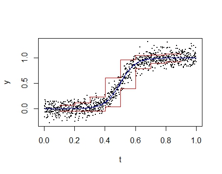
((a)) $m_{1}(t)=1/(1+e^{-20(t-0.5)})$

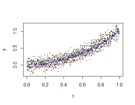
((b)) $m_{2}(t)=t^{2}$

Figure 2: 90% confidence bands

6.3 Analysis of Global Temperature Anomaly and Internet Usage Data

We apply our methodology to two data sets, one exhibiting short- and the other long-range dependence. In the former case we use the $L_{n}$ statistic and in the latter the ratio based statistic $\Psi_{n}$.

Global Temperature Anomaly Data (Short-range dependence)

We consider the global warming data used in ZW[47], which consists of global annual temperature anomalies, measured in degrees celsius from 1850 to 2009. These anomalies are, simply, temperature deviations measured with respect to the base period 1961-1990. The autocorrelation plot of these data suggests that the dependence can be well accounted for using an AR(2) process, see ZW[47]. The short-range dependence condition (6) applies to AR(2) time series. Figures 3(a) and 3(b) represent the data along with its isotonic regression estimates and 90% confidence intervals and band respectively obtained by using $L_{n}$. The estimate of the asymptotic standard deviation $\tau$ was taken to be $0.1248$ from Wu et. al. (2001)[45]. Note that the point-wise confidence intervals in the left panel form a rather smooth band, which mimics, in shape, the isotonic regression curve but should not be confused with the uniform confidence band in the right panel which is naturally wider. Apart from the estimate of $\tau$, our methodology is completely agnostic to the nature of short-range dependence and regularity of the trend. As can be seen from the two figures, our confidence intervals show some (data-based) evidence for systematic growth of the global temperature anomalies, as should be expected, given the compelling evidence from numerical climate model simulations of the Intergovernmental Panel of Climate Change IPCC (2007)[19]. We compare our point-wise confidence intervals method with those obtained by kernel smoothing ignoring the monotonicity constraint as decribed in Robinson (1997)[33]. Following the example described in Section 5 of that paper, we use the kernel $k(x)=[1/2(1+\cos(\pi x))]\mathbf{1}(|x|\leq 1)$ and the three fixed bandwidths used therein: $b=.05,.075,.1$ for the regression estimator. We use the differencing method, equation (4.6) (with the same kernel $l=k$ and the same three bandwidths ($c=b$)), along with the formulas in equation (4.10) of that paper to estimate the asymptotic variance. Note that Robinson’s set-up assumes Lipschitz continuity of the regression function and its derivative, which is stronger than the assumptions underlying our isotonic procedure. Figure 4(b) shows these point-wise CIs for $b=c=0.05$ (the other bandwidths produced similar results) with the isotonic point-wise CIs being plotted alongside in Figure 4(a) for convenience of comparison. The pattern of the CIs using Robinson’s method is similar to those obtained by the isotonic procedure for the latter half of the time period when the monotonicity of the trend is more pronounced. The different behavior of the two estimators in the earlier time period can be accounted for by noticing that our procedure enforces global monotonicity while Robinson’s does not.

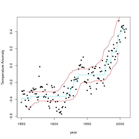
((a)) Point-wise confidence intervals

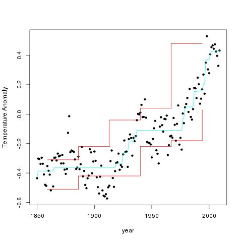
((b)) Confidence band

Figure 3: 90% confidence intervals and confidence band for global temperature anomaly data

((a)) Point-wise confidence intervals using $L_{n}$

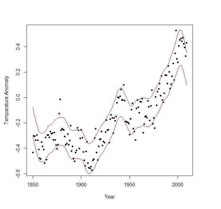
((b)) Point-wise confidence intervals using kernel smoothing

Figure 4: 90% point-wise confidence intervals for global temperature anomaly data

Internet Traffic Data (Long-range dependence)

This example involves computer network traffic data obtained from the Internet2 network [3]. The data consists of number of bytes per 100 millisecond time-intervals over a fast backbone link measured on 17th March, 2009. Such traffic traces exhibit typical diurnal patterns with clearly defined periods of monotone non-decreasing or non-increasing trends throughout the day. This is associated with usual growth/decay of the number of active users in the beginning/middle of the day. Further, it is well known and documented that Internet traffic traces exhibit long-range dependence (see e.g. Willinger et. al. (1995)[43] and Stoev et. al. (2005)[39]). Such data provide an ideal test-bed for the performance of our confidence intervals based on the ratio statistic. To be able to provision network capacity as well as detect anomalous network activity, it is important to have accurate estimates of confidence intervals that are robust to the presence of long-range dependence and account for natural traffic trends, without imposing stringent parametric/smoothness assumptions. This is particularly important in the network traffic context, where unusual changes in the regularity of the trend may occur and methods that involve estimation of derivatives require great care to implement and, in fact, can lead to non-robust interval estimates.

We focused on the time period $11:06$ to $16:36$ GMT, corresponding to $7:06$ AM to $12:36$ AM in US EST, where there is a typical monotone non-decreasing diurnal trend due to systematic increase of the number of active users in the beginning of the day. The Hurst parameter was estimated to be $\hat{H}=0.9491$ using wavelet methods[39].

Figure 5(a) shows 90% point-wise confidence intervals at 50 time points based on the $\Psi_{n}$ statistic with $H=0.95$. Observe that the confidence intervals (which are joined across time) generally track the monotone trend but should not be interpreted as uniform bands. In contrast to the intervals based on the $L_{n}$ and $T_{n}$ statistics, the intervals based on $\Psi_{n}$ are not smooth over time. Since we have not performed any smoothing, nor aimed to produce a confidence band, this feature is not alarming. This irregularity of the proposed confidence intervals is yet to be fully understood, theoretically. Since $\Psi_{n}$ is obtained as a non-linear, ratio functional of the discrepancy statistics $L_{n}$ nor $T_{n}$, the joint behavior of $L_{n}$ and $T_{n}$ near zero should play a key role. Regardless of the unusual irregularity feature, our confidence estimates provide reliable coverage and are nearly dependence-universal, as confirmed by our theory and extensive simulation studies only some of which are reported.

We compare our intervals to Figure 5(b) which provides point-wise confidence intervals at the same 50 time points using the method in Robinson (1997) [33]. The details of the construction remain the same as in the short-range dependence case described previously, the only difference being that $\hat{H}$ and $\hat{G}$ appearing in the asymptotic variance are now computed using the raw data, i.e. $\hat{u}_{t}=Y_{t}$ as in (4.12) of Robinson’s paper instead of the formula (4.6) used under short-range dependence. The estimated $\hat{H}$ based on the alternative method is 0.9502, close to our obtained estimate $0.9491$. The most striking difference between this kernel method and ours is that the length of the confidence intervals constructed by the kernel method remains the same for all the 50 points, since the asymptotic variance of the estimator of $m(x)$ does not depend on $x$ therein. Our confidence intervals appear to be reacting more keenly to the variability in the data relative to the slope of the trend curve.

Section 6 and Table 7 in Supplement A present some limited studies of the coverage properties of the kernel based CIs for the same two functions $m_{1}$ and $m_{2}$ in (25), which we used to study our proposed methods. As is evident from the table, the kernel based CIs suffer from considerable under-coverage for the ill-behaved $m_{2}$ and especially so under strong dependence, similar to the IRE based intervals reported in other tables. Thus, while being visually more appealing (smother) than the $\Psi_{n}$ based CIs, the kernel based CIs are not accurate for ill-behaved trend functions and the $\Psi_{n}$ based ones remain substantially more reliable in such cases.

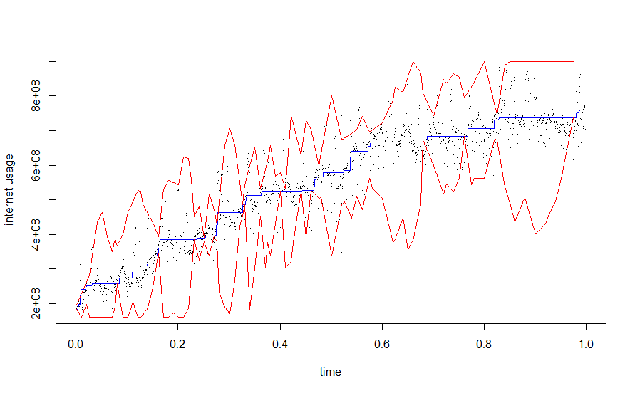
((a)) Point-wise confidence intervals using $R_{n}$

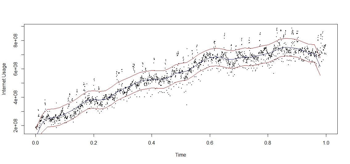
((b)) Point-wise confidence intervals using kernel smoothing

Figure 5: 90% point-wise confidence intervals for internet traffic data

Appendix A Proof-sketch of asymptotics of the test statistics $L_{n}$ and $T_{n}$:

The statistics $L_{n}$ and $T_{n}$ are determined by the discrepancy between $\hat{m}_{n}(t)$ and $\hat{m}_{n}^{0}(t)$ in the neighborhood of $t_{0}$ over which they differ.
We focus on a shrinking neighborhood of $t_{0}$ at rate $d_{n}\downarrow 0$, which will determined by the type of dependence structure of the error sequence, since $\hat{m}_{n}$ and $\hat{m}_{n}^{0}$ are equal outside of neighborhoods of this order of magnitude. For example, under independence or short-range dependence $d_{n}\sim n^{-1/3}$, while under long-range dependence the rate will involve the Hurst index. More formally, let $z:=d_{n}^{-1}(t-t_{0})$ and define

$$X_{n}(z)=\frac{1}{d_{n}}\left(\hat{m}_{n}\left(t_{0}+zd_{n}\right)-\theta_{0}\right)\mbox{ and }Y_{n}(z)=\frac{1}{d_{n}}\left(\hat{m}_{n}^{0}\left(t_{0}+zd_{n}\right)-\theta_{0}\right),$$ (26)

for $z\in(a_{n},b_{n}]:=(-d_{n}^{-1}t_{0},d_{n}^{-1}(1-t_{0})]$. Here $\theta_{0}=m(t_{0})$. It turns out that the statistics $L_{n}$ and $T_{n}$ can be represented asymptotically as fairly simple integrals involving $X_{n}$ and $Y_{n}$ and also that the set of $z$’s on which they differ is contained, with high probability, in a compact set. These are the contents of the two results stated below.

Proposition A.1.

For $L_{n}$ and $T_{n}$ as in (4), we have

$$L_{n} = \frac{n^{2}d_{n}^{3}}{\sigma_{n}^{2}}{\Big{(}}\int_{(a_{n},b_{n}]}\left(X_{n}^{2}(z)-Y_{n}^{2}(z)\right)dz+o_{P}(1){\Big{)}}$$ (27)

$$T_{n} = \frac{n^{2}d_{n}^{3}}{\sigma_{n}^{2}}{\Big{(}}\int_{(a_{n},b_{n}]}\left(X_{n}(z)-Y_{n}(z)\right)^{2}dz+o_{P}(1){\Big{)}}.$$

Lemma A.1.

Let $D_{n}:=\{z\in\mathbb{R}\,:\,X_{n}(z)\not=Y_{n}(z)\}$. For any $\epsilon>0$, there exist $M_{\epsilon}>0$ and $n_{\epsilon}>0$, such that

$$\mathbb{P}{\Big{(}}D_{n}\subset[-M_{\epsilon},M_{\epsilon}]{\Big{)}}\geq 1-\epsilon,$$

for all $n\geq n_{\epsilon}.$

The proofs of the preceding proposition and lemma are given in Section 2.2 of Supplement A.
It is then clear that fathoming the asymptotic behavior of $L_{n},T_{n}$ requires an understanding of the asymptotic behavior of the processes $(X_{n},Y_{n})$ on compact sets, since with high probability, the difference set $D_{n}$ is contained in a compact set. If we could show that $(X_{n},Y_{n})$ converge to limit processes $(X_{\infty},Y_{\infty})$ with increasing sample size on every compact set (in a strong-enough metric under which integral type functionals are continuous), then, roughly speaking, up to adequate normalizations our limits for $L_{n}$ and $T_{n}$ should have forms:

$$\int\,(X_{\infty}^{2}(z)-Y_{\infty}^{2}(z))\,dz\;\;\mbox{and}\;\;\int\,(X_{\infty}(z)-Y_{\infty}(z))^{2}\,dz\,,$$ (28)

respectively. It turns out that the topology of $L^{2}$ convergence on compact sets is adequate for this purpose.
The processes $X_{n}$ and $Y_{n}$ can be represented as greatest convex minorant functionals of a normalized version of the the process $U_{n}$, the linear interpolation of the cumulative sum process of the $Y_{i}$’s, namely:

$$U_{n}(t)=\frac{Y_{1}+Y_{2}+\dots+Y_{\lfloor nt\rfloor}}{n}+\frac{(nt-\lfloor nt\rfloor)}{n}Y_{\lfloor nt\rfloor+1},\;t\in[0,1]\,.$$ (29)

More specifically, defining:

$$\mathbb{V}_{n}(z):=d_{n}^{-2}\Big{(}U_{n}(t_{0}+d_{n}z)-U_{n}(t_{0})-m(t_{0})d_{n}z\Big{)},\hskip 14.45377ptz\in(a_{n},b_{n}]\,,$$ (30)

we can write:

$$X_{n}(z)= \mathcal{L}\circ\mathcal{T}_{(a_{n},b_{n}]}\left(\mathbb{V}_{n}\right)(z)$$ (31)

$$Y_{n}(z)= \left(\mathcal{L}\circ\mathcal{T}_{(a_{n},l_{n}]}\left(\mathbb{V}_{n}\right)(z)\wedge 0\right)\mathbf{1}_{(a_{n},l_{n}]}(z)+0\times\mathbf{1}_{(l_{n},0]}(z)$$

$$+\left(\mathcal{L}\circ\mathcal{T}_{(l_{n},b_{n}]}\left(\mathbb{V}_{n}\right)(z)\vee 0\right)\mathbf{1}_{(0,b_{n}]}(z),$$

where $l_{n}=d_{n}^{-1}(t_{l}-t_{0})$. (Recall that the operators involved in the definition of $X_{n}$ and $Y_{n}$ were introduced in Section 4.) This is a direct consequence of the well-known representation of $\hat{m}_{n}$ and $\hat{m}_{n}^{0}$ in terms of $U_{n}$ (see (2.1) in Supplement A) followed by an appropriate renormalization. The limiting properties of $(X_{n},Y_{n})$ are therefore driven by those of $\mathbb{V}_{n}$, which is fortunately well-studied (AH [2]). More concretely, we know:

Theorem A.1.

Consider the processes $\mathbb{V}_{n}$ in the space $C(\mathbb{R})$ equipped with the topology of uniform convergence on compact sets. Then, as $n\to\infty$,

$$\mathbb{V}_{n}\Longrightarrow\{\mathbb{G}(z)\}_{z\in\mathbb{R}}\equiv\{\mathbb{G}_{a,b}(z)\}_{z\in\mathbb{R}}:=\{a\mathbb{W}(z)+bz^{2}\}_{z\in\mathbb{R}},$$ (32)

where $b=\frac{1}{2}m^{\prime}(t_{0})$ and (i) (under weak dependence) $d_{n}=n^{-\frac{1}{3}},$ $\mathbb{W}$ is a two-sided Brownian motion on $\mathbb{R}$, and $a:=\tau$ given in (8).
(ii) (under strong dependence) $d_{n}=l_{2}(n)n^{-\frac{d}{2+d}},$ $\mathbb{W}$ is the fBm process $B_{H}$ and $a:=|\eta_{1}|$. (Here $l_{2}$ is a slowly varying function related to $l_{1}$ as shown in the proof of the theorem, provided in Supplement A.)

We therefore expect $(X_{\infty},Y_{\infty})$ the limits of $(X_{n},Y_{n})$ to be given by replacing $a_{n},b_{n},l_{n},\mathbb{V}_{n}$ by their corresponding limits in (31). But these are precisely $(\mathcal{S}_{a,b}(z),\mathcal{S}_{a,b}^{0}(z))$ introduced in Section 4.
We next define the space $L^{2}_{loc}$ which appears in the formal statement of convergence of $(X_{n},Y_{n})$. This is the space of all functions which are square integrable on compact sets. The convergence in this space is accordingly defined, that is, a sequence of functions $f_{n}\to f$ as $n\to\infty$ in $L^{2}_{loc}$ if $\int_{I}(f_{n}-f)^{2}\to 0$ as $n\to\infty$ for every compact interval $I$. In fact with this convergence the space is metrizable. We have:

Theorem A.2.

As $n\to\infty$, we have

$$\{(X_{n}(z),Y_{n}(z))\}_{z\in\mathbb{R}}\Longrightarrow\{(\mathcal{S}_{a,b}(z),\mathcal{S}_{a,b}^{0}(z))\}_{z\in\mathbb{R}}\ \ \mbox{ in }L^{2}_{loc}\times L^{2}_{loc},$$ (33)

where the components of the limit process are defined in (12).

The formal proof of this theorem is highly technical and provided in Supplement A. The above result coupled with the forms of the expressions in (28) immediately lead to the forms for $L_{a,b}$ and $T_{a,b}$ given in (17).

Appendix B Proof of Theorem 4.2

We first state a version of the converging together lemma which is used later, and is an adaptation of Theorem 8.6.2 in Resnick (1999)[32].

Lemma B.1.

Let $\xi,\xi_{\delta,c,n},\ \xi_{\delta,c},\ \eta_{n},\ n\in\mathbb{N},\delta,\ c>0$ be random elements taking values in a metric space $(E,d)$. If (i) $\xi_{\delta,c,n}\Rightarrow\xi_{\delta,c}$, as $n\to\infty$, (ii) $\xi_{\delta,c}\Rightarrow\xi$, as $c\to\infty$ and $\delta\uparrow 0$ and (iii) for all $\epsilon>0$,

$$\lim_{\delta\uparrow 0}\lim_{c\to\infty}\limsup_{n\geq 1}\mathbb{P}(d(\xi_{\delta,c,n},\eta_{n})>\epsilon)=0,$$ (34)

then $\eta_{n}\Rightarrow\xi$, as $n\to\infty$.

Proof of Theorem 4.2 By Lemma A.1 and Theorem 3.1 (Supplement B), for every $\epsilon>0$ there exists an interval $K_{\epsilon}:=[-M_{\epsilon},M_{\epsilon}]$ such that, for all large $n$,

$$\mathbb{P}\Big{[}D_{n}\subset[-M_{\epsilon},M_{\epsilon}]\Big{]}>1-\epsilon\mbox{ and }\mathbb{P}\Big{[}D_{a,b}\subset[-M_{\epsilon},M_{\epsilon}]\Big{]}>1-\epsilon.$$

Let now

$$\xi_{\epsilon,n}={\Big{(}}\int_{K_{\epsilon}}\Big{(}X_{n}^{2}(z)-Y_{n}^{2}(z)\Big{)}dz,\,\int_{K_{\epsilon}}\Big{(}X_{n}(z)-Y_{n}(z)\Big{)}^{2}dz{\Big{)}},$$

$$\xi_{\epsilon}={\Big{(}}\int_{K_{\epsilon}}\Big{(}(\mathcal{S}_{a,b}(z))^{2}-(\mathcal{S}_{a,b}^{0}(z))^{2}\Big{)}dz,\,\int_{K_{\epsilon}}\Big{(}\mathcal{S}_{a,b}(z)-\mathcal{S}_{a,b}^{0}(z)\Big{)}^{2}dz{\Big{)}}.$$

Also, let

$$\eta_{n}={\Big{(}}\int_{(a_{n},b_{n}]}\Big{(}X_{n}^{2}(z)-Y_{n}^{2}(z)\Big{)}dz,\ \int_{\mathbb{R}}\Big{(}X_{n}(z)-Y_{n}(z)\Big{)}^{2}dz{\Big{)}},$$

$$\xi={\Big{(}}\int_{D_{a,b}}\Big{(}(\mathcal{S}_{a,b}(z))^{2}-(\mathcal{S}_{a,b}^{0}(z))^{2}\Big{)}dz,\,\int_{D_{a,b}}\Big{(}\mathcal{S}_{a,b}(z)-\mathcal{S}_{a,b}^{0}(z)\Big{)}^{2}dz{\Big{)}}.$$

Since $K_{\epsilon}$ contains $D_{n}:=\{z\,:\,X_{n}(z)\not=Y_{n}(z)\}$ with probability greater than $1-\epsilon$ and $(a_{n},b_{n}]$ grows up to $\mathbb{R}$, for large $n$, we have $\lim_{\epsilon\downarrow 0}\limsup_{n\geq 1}\mathbb{P}(\xi_{\epsilon,n}\neq\eta_{n})=0$. We similarly have that $\lim_{\epsilon\downarrow 0}\mathbb{P}(\xi_{\epsilon}\neq\xi)=0$. Finally, by Theorem A.2 and the continuous mapping Theorem, for all fixed $\epsilon>0$, we have $\xi_{\epsilon,n}\Rightarrow\xi_{\epsilon}$, as $n\to\infty$. Thus, all conditions of the converging together lemma (cf Lemma B.1) hold, where in this simple case there is no dependence on $\delta>0$. Hence $\eta_{n}\Rightarrow\xi,\ n\to\infty$, which, in view of Proposition A.1, yields

$$\frac{\sigma_{n}^{2}}{n^{2}d_{n}^{3}}(L_{n},T_{n})\Longrightarrow\left(\mathbb{L}_{a,b}^{(H)},\mathbb{T}_{a,b}^{(H)}\right)$$

as $n\to\infty$.

To complete the proof, it remains to show that

$$\left(\mathbb{L}_{a,b}^{(H)},\mathbb{T}_{a,b}^{(H)}\right)\stackrel{{\scriptstyle d}}{{=}}a^{2}\left(\frac{a}{b}\right)^{\frac{2H-1}{2-H}}\left(\mathbb{L}^{(H)},\mathbb{T}^{(H)}\right).$$ (35)

This follows from a scaling argument. Indeed, by the $H$-self-similarity of $B_{H}$, for $\mathbb{G}(z)\equiv\mathbb{G}_{a,b}^{H}(z)=a{B}_{H}(z)+bz^{2}$, we have

$$\{\mathbb{G}_{a,b}^{H}(z)\}_{z\in\mathbb{R}}\stackrel{{\scriptstyle d}}{{=}}a(a/b)^{\frac{H}{2-H}}{\Big{\{}}{\Big{(}}\mathbb{G}_{1,1}^{H}((b/a)^{\frac{1}{2-H}}z){\Big{)}}{\Big{\}}}_{z\in\mathbb{R}}.$$ (36)

Thus, the process $\{(\mathcal{S}_{a,b}(z),\mathcal{S}_{a,b}^{0}(z))\}_{z\in\mathbb{R}}$ equals in distribution

$$a\left(b/a\right)^{\frac{1-H}{2-H}}{\Big{\{}}{\Big{(}}\mathcal{S}_{1,1}(\left(b/a\right)^{\frac{1}{2-H}}z),\,\mathcal{S}_{1,1}^{0}(\left(b/a\right)^{\frac{1}{2-H}}z){\Big{)}}{\Big{\}}}_{z\in\mathbb{R}},$$ (37)

which by substituting in (17) and making a change of variables yields (35). $\Box$

Remark B.1.

The result of Theorem 4.1 can be formally recovered from the statement of Theorem 4.2 by letting $H=1/2$, $a=\tau$, $d_{n}=n^{-1/3}$, using the fact that $\sigma_{n}^{2}/n\rightarrow\tau^{2}$ and noting that $\mathbb{L}^{(1/2)}$ and $\mathbb{T}^{(1/2)}$ are precisely the $\mathbb{L}$ and $\mathbb{T}$ of Theorem 4.1 respectively.

Appendix C Supplementary Materials

Supplement A:

Supplement containing technical details and proofs of the results stated in the paper

Supplement B:

Technical report containing properties of some important functionals Brownian and fractional Brownian motion in context of shape restricted regression. This file also contains properties and simulation of the random variables appearing in the limit distribution of the statistics used in this paper.

References

- Arby and Veitch [1998] Abry, P. and Veitch, D. (1998) Wavelet analysis of long-range dependent traffic. Institute of Electrical and Electronics Engineers. Transactions on Information Theory Vol. 44, No. 1, 2-15.
- Anevski and Hossjer [2006] Anevski, D. and Hossjer, O.(2006) A general asymptotic scheme for inference under order restrictions. The Annals of Statistics Vol. 34, 1874-1930.
- [3] Backbone link traces from the Internet2 network http://www.internet2.edu/
- Banerjee and Wellner [2001] Banerjee, M. and Wellner, J. A.(2001) Likelihood ratio tests for monotone functions. The Annals of Statistics Vol. 29, 1699-1731.
- Banerjee and Wellner [2005] Banerjee, M. and Wellner, J. A.(2005) Confidence intervals for current status data. Scandinavian Journal of Statistics Vol. 32 405-424.
- Banerjee [2007] Banerjee, M.(2007) Likelihood based inference for monotone response models. Annals of Statistics Vol 35, No. 3 931–956.
- Banerjee [2009] Banerjee, M. (2009) Inference in exponential family regression models under certain shape constraints. Advances in Multivariate Statistical Methods, Statistical Science and Interdisciplinary Research, Vol. 4, 249-272. World Scientific.
- Brunk [1970] Brunk, H. D. (1970) Estimation of isotonic regression. In Nonparametric Techniques in Statistical Inference (M. L. Puri, ed,) 177-197. Cambridge University Press, London.
- Clifford et. al. [2005] Clifford, H., Lang, G. and Soulier, P . (2005). Estimation of long memory in the presence of a smooth nonparametric trend. J. Amer. Statist. Assoc., Vol 100, no. 471, 853-871.
- Doukhan et. al. [2003] Doukhan, P., Oppenheim, G. and Taqqu, M. S. (2003). Theory and applications of long-range dependence., Birkhäuser Boston Inc., Boston, MA
- Fan and Yao [2003] Fan, J. and Yao, Q. (2003) Nonlinear Time Series. Nonparametric and Parametric Methods Series: Springer Series in Statistics.
- Fay et. al. [2009] Fay, G., Moulines, E., Roueff, F. and Taqqu, M. S. (2009). Estimators of long-memory: Fourier versus wavelets. Journal of Econometrics Vol. 151, No. 2 159-177.
- Groeneboom [1985] Groeneboom, P. (1985). Estimating a monotone density. Proceeding of the Berkeley Conference in Honor of Jezry Neyman and Jack Kiefer Vol II, (Lucien, M. LeCam and Richard A. Olshen eds.)
- Groeneboom [2003] Groeneboom, P. and Jongbloed, G. (2003). Density estimation in the uniform deconvolution model. Statistica Neerlandica Vol. 57 136-157.
- Groeneboom and Wellner [1992] Groeneboom, P. and Wellner J.A. (1992). Information Bounds and Nonparametric Likelihood Estimation. Birkhauser, Basel.
- Groeneboom and Wellner [2001] Groeneboom, P. and Wellner J.A. (2001). Computing Chernoff’s distribution. Journal of Computational and Graphical Statistics. Vol. 10, 388-400.
- Haslett and Raftery [1989] Haslett J. and Raftery A.E. (1989). Space-Time Modelling with Long-Memory Dependence: Assessing Ireland’s Wind Power Resource. Applied Statistics Vol. 38, 1-50.
- Hussian et. al. [2005] Hussian, M., Grimvall, A., Burdakov, O. and Sysoev O. (2005). Monotonic regression for the detection of temporal trends in environmental quality data. Communications in Mathematical and in Computer Chemistry Vol. 54, 535-550.
- IPCC [2007] IPCC (2007). Nobel Peace Prize, Intergovernmental Panel on Climate Change - Facts. Nobelprize.org. Nobel Media AB 2014. Web. 12 Dec 2014. http://www.nobelprize.org/nobel_prizes/peace/laureates/2007/ipcc-facts.html
- Jones and Mann [2004] Jones, P. D., and Mann, M. E. (2004). Climate over past millennia. Reviews of Geophysics, Vol. 42) RG2002
- Mammen [1991] Mammen, E. (1991). Estimating a Smooth Monotone Regression Function. The Annals of Statistics Vol 19 724-740.
- Meal [2011] Meal, D. (2011). Statistical Analysis for Monotone Trend. The NCSU Water Quality Group Newsletter Issue 135 1-11
- Memendez et. al. [2013] Memendez, P.; Ghosh, S.; Hans, R. K. and Tinner, W. (2013). On trend estimation under monotone Gaussian subordination with long-memory: application to fossil pollen series. Journal of Nonparametric Statistics Vol 25 765-785
- Moulines et. al. [2008] Moulines, E., Roueff, F., and Taqqu, M. S. (2008). A wavelet whittle estimator of the memory parameter of a nonstationary Gaussian time series. The Annals of Statistics, 1925-1956.
- Mukherjee [1988] Mukherjee, H. (1988). Monotone Nonparametric Regression. The Annals of Statistics Vol 16 741-750.
- NAAQS [1990] NAAQS (1990). National Ambient Air Quality Standards (NAAQS), Amendment to the “Clean Air Act" http://www.epa.gov/air/criteria.html.
-
[27]
NASA GISS Surface Temperature Analysis
http://data.giss.nasa.gov/gistemp/graphs_v3/ - Pal and Woodroofe [2007] Pal, J. and Woodroofe, M. (2007). Large Sample Properties of Shape Restricted Regression Estimators With Smoothness Adjustments. Statistics Sinica, Vol. 17, 1601-1616.
- Peligrad and Utev [2005] Peligrad, M. and Utev, S. (2005). A new maximal inequality and invariance principle for stationary sequences. The Annals of Probability Vol. 33, 798-815.
- Ramsay [1998] Ramsay, J.O.(1998). Estimating Smooth Monotone Functions. Journal of the Royal Society: Series B Vol. 60, 365-375.
- Rao [1969] Rao, P.B.L.S.(1969). Estimation of unimodal density. Sankhya Ser. A Vol 31, 23-36.
- Resnick [1999] Resnick, S. I.(1999). A Probability Path. Birkhäuser, Boston.
- Robinson [1997] Robinson, P. M. (1997). Large-sample inference for nonparametric regression with dependent errors. The Annals of Statistics, Vol. 25 no. 5, 2054-2083.
- Robertson et. al. [1988] Robertson, T., Wright, F. T. and Dykstra, R. L.(1988). Order Restricted Statistical Inference. New York: Wiley.
- Robinson [2009] Robinson, P. M. (2009) Inference on nonparametrically trending time series with fractional errors. Econometric Theory, Vol. 25, no. 6, 1716-1733.
- Rockafeller [1970] Rockafellar, R.T.(1970). Convex Analysis. Princeton University Press, Princeton.
- Samorodnitsky [2006] Samorodnitsky, G (2006). Long range dependence. Foundations and Trends® in Stochastic Systems, Vol. 1, No. 3, 163–257.
- Steig et. al. [2009] Steig, E., Schneider, D., Rutherford, S., Mann, M., Comiso, J., and Shindell, D. (2009). Warming of the Antarctic ice-sheet surface since the 1957 International Geophysical Year. Nature Vol. 457, 459-463.
- Stoev et. al. [2005] Stoev, S. A., Taqqu, M. S., Park, C., Marron, J. S. (2005). On the wavelet spectrum diagnostic for Hurst parameter estimation in the analysis of Internet traffic. Computer Networks, 48, 423-445.
- Sun and Woodroofe [1996] Sun, J. and Woodroofe, M.(1996) Adaptive smoothing for a penalized NPMLE of a non-increasing density. Journal of Statistical Planning and Inference Vol. 52, 143-159.
- Taqqu [1975] Taqqu, M. S. (1975). Weak convergence to fractional Brownian motion and to Rosenblatt process. Z. Wahrsch. Verw. Gebiete Vol. 31, 287-302.
- Taqqu [1979] Taqqu, M. S. (1979). Convergence of integrated processes of arbitrary Hermite rank. Z. Wahrsch. Verw. Gebiete Vol. 50, 53-80.
- Willinger et. al. [1995] Willinger, W., Taqqu, M.S., Leland, W. E., and Wilson, V. (1995). Self-Similarity in high-speed packet traffic: analysis and modeling of Ethernet traffic measurements. Statistical Science, 10, 67-85.
- Woodroofe and Sun [1993] Woodroofe, M. and Sun, J. (1993) A penalized maximum likelihood estimate of when is non-uncreasing. Statistica Sinica Vol. 3, 501-515.
- Wu et. al. [2001] Wu, W. B., Woodroofe, M. and Mentz, G. (2001) Isotonic regression: another look at the change point problem. Biometrika Vol. 88, 793-804.
- Wu and Zhao [2007] Wu, W.B. and Zhao, Z. (2007). Inference of trends in time series. J. R. Stat. Soc. Ser. B, Vol. 69, no. 3, 391-410.
- Zhao and Woodroofe [2012] Zhao, O. and Woodroofe, M.(2012) Estimating a monotone trend. Statistica Sinica, Vol. 22, 359-378.