A Limit Formula for Joint Spectral Radius with $p$-radius of Probability Distributions

Abstract

In this paper we show a characterization of the joint spectral radius of a set of matrices as the limit of the $p$-radius of an associated probability distribution when $p$ tends to $\infty$. Allowing the set to have infinitely many matrices, the obtained formula extends the results in the literature. Based on the formula, we then present a novel characterization of the stability of switched linear systems for an arbitrary switching signal via the existence of stochastic Lyapunov functions of any higher degrees. Numerical examples are presented to illustrate the results.

1 Introduction

The joint spectral radius of a set of matrices, originally introduced in the short note [1], is a natural extension of the spectral radius of a single matrix and has found various applications in, for example, wavelet theory, functional analysis, and systems and control theory (see the monograph [2] for detail). This wide range of applications has motivated many authors to study the computation of joint spectral radius. Though even the approximation of joint spectral radius is in general an NP-hard problem [3], there are now a vast amount of efficient methods for the approximation of joint spectral radius [4, 5, 6] and also their implementations on mathematical softwares [7].

The result [4] by Blondel and Nesterov is of a particular theoretical interest because it characterizes joint spectral radius as the limit of another joint spectral characteristics called $L^{p}$-norm joint spectral radius when $p$ tends to $\infty$. Given a finite set $\mathcal{M}=\{A_{1},\dotsc,A_{N}\}$ of real and square matrices of a fixed dimension and a parameter $p\geq 1$, the $L^{p}$-norm joint spectral radius ($p$-radius for short) of $\mathcal{M}$ is defined by

$$\rho_{p,\mathcal{M}}:=\lim_{k\to\infty}\biggl{(}N^{-k}\sum_{i_{1},\dots,i_{k}\in\{1,\dotsc,N\}}\lVert{A_{i_{k}}\dotsm A_{i_{1}}}\rVert^{p}\biggr{)}^{1/kp},$$ (1)

where $\lVert{\cdot}\rVert$ denotes any matrix norm. Firstly introduced [8, 9] for $p=1$ and then extended [10] for a general $p$, $L^{p}$-norm joint spectral radius has found many applications in various areas of applied mathematics (see [11] and references therein). In particular $p$-radius has an application to the stability theory of stochastic switched systems [12, 13, 14], which is a dynamical system whose structure randomly experiences abrupt changes [15, 16].

Recently this “original” version of $L^{p}$-norm joint spectral radius was extended to probability distributions [13]. Roughly speaking, the extension makes it possible to consider the $p$-radius of a set of infinitely many matrices and is useful when, for example, one wants to study the stability of a stochastic switched system with infinitely many subsystems that naturally arise as a result of uncertainty in modeling of dynamical systems. Being an extension, the $p$-radius of distributions inherits [13] from the $p$-radius of sets of matrices the characterization [10] as the spectral radius of a matrix. Though the characterization is valid only either when $p$ is an even integer or when matrices in $\mathcal{M}$ leave a common proper cone invariant, it still covers several interesting cases that appear in the stability analysis of stochastic switched linear systems. Then it is natural to expect that the other properties of the $p$-radius of sets of matrices can be extended to the $p$-radius of distributions.

In this paper we show that the characterization by Blondel and Nesterov [4] is still valid when we use the $p$-radius of probability distributions. This extension in particular circumvents the finiteness limitation of the original characterization. Since the proof for the original result relies on the finiteness of the number of matrices, it cannot be directly applied to the current setting. Instead, our proof extensively utilizes so-called cone linear absolute norms [17] and the approximation of a given set of possibly infinitely many matrices by subsets having a certain uniformity property.

As a theoretical application of the characterization of joint spectral radius, we will discuss the stability of switched linear systems. We will present a novel characterization of the stability of a switched linear system for an arbitrary switching signal with a so-called stochastic Lyapunov function [18, 19, 20], which is a positive definite functional whose value decreases along the trajectory of the switched linear system in expectation. The characterization in particular deduces the existence of stochastic Lyapunov functions from stability and hence is a variant of the converse Lyapunov theorems [21, 22] in systems and control theory. The construction of stochastic Lyapunov functions is also investigated.

This paper is organized as follows. After preparing necessary notations in Section 2, in Section 3 we give a brief overview of the joint spectral radius of sets of matrices and the $L^{p}$-norm joint spectral radius of probability distributions. Then Section 4 gives the characterization of joint spectral radius as the limit of $L^{p}$-norm joint spectral radius. In Section 5 we discuss the application of the characterization to the stability theory of switched linear systems.

2 Mathematical Preliminaries

Let $\mathbb{R}_{+}$ denote the set of nonnegative real numbers. For $x\in\mathbb{R}^{n}$ its Euclidean norm is denoted by $\lVert{x}\rVert$, if not explicitly stated otherwise. For a real matrix $A$ its maximal singular value is denoted by $\lVert{A}\rVert$. If $A$ is square then its spectral radius is denoted by $\rho(A)$. When $A$ is symmetric and negative semidefinite we write $A\preceq 0$. Let $\mathcal{M}\subset\mathbb{R}^{n\times n}$. The interior and the boundary of $\mathcal{M}$ are denoted by $\operatorname{int}\mathcal{M}$ and $\partial\mathcal{M}$, respectively. The distance between $A$ and $\mathcal{M}$ is defined by $d(A,\mathcal{M}):=\inf_{M\in\mathcal{M}}\lVert{A-M}\rVert$.

Let $\Omega$ be a probability space with a probability measure $\mu$. The support of $\mu$, denoted by $\operatorname{supp}\mu$, is defined as the closed set such that $\mu((\operatorname{supp}\mu)^{c})=0$ and, if $G$ is open and $G\cap{(\operatorname{supp}\mu)}\neq\emptyset$, then $\mu(G\cap\operatorname{supp}\mu)>0$. Dirac’s delta distribution on $x\in\Omega$ is denoted by $\delta_{x}$. For an integrable random variable $X$ on $\Omega$ its expected value is denoted by $E[X]$.

2.1 Proper Cones

A subset $K\subset\mathbb{R}^{n}$ is called a cone if $K$ is closed under multiplication by nonnegative numbers. The cone is said to be solid if it possesses a nonempty interior. We say that a cone is pointed if $x,-x\in K$ implies $x=0$. We say that $K$ is proper if it is closed, convex, solid, and pointed. Let $K\subset\mathbb{R}^{n}$ be a proper cone. A matrix $A\in\mathbb{R}^{n\times n}$ is said to leave $K$ invariant, written $A\geq^{K}0$, if $AK\subset K$. The set of all real matrices leaving $K$ invariant is denoted by $\pi(K)$ or simply by $\pi$. Let $B\in\mathbb{R}^{n\times n}$. By $A\geq^{K}B$ we mean $A-B\geq^{K}0$. A set $\mathcal{M}\subset\mathbb{R}^{n\times n}$ is said to leave $K$ invariant if any $A\in\mathcal{M}$ leaves $K$ invariant. $A$ is said to be $K$-positive if $A(K-\{0\})\subset\operatorname{int}K$ and we write $A>^{K}0$. We understand $A>^{K}B$ in the obvious way. It is known that [24, p. 16]

$$\operatorname{int}\pi=\{A\in\mathbb{R}^{n\times n}:A>^{K}0\}.$$ (2)

Also we can show the next lemma.

Lemma 2.1.

The boundary $\partial\pi$ is a null set with respect to the Lebesgue measure.

Proof.

In general, the boundary of a convex set in $\mathbb{R}^{n\times n}$ is a null set with respect to the Lebesgue measure [23, Theorem 1]. This proves the claim because $\pi$ is clearly convex. ∎

A class of norms called cone linear absolute norms (see, e.g., [17]) plays an important role in this paper. A norm $\lVert{\cdot}\rVert$ on $\mathbb{R}^{n}$ is said to be cone absolute [17] with respect to a proper cone $K$ if, for every $x\in\mathbb{R}^{n}$,

$$\lVert{x}\rVert=\inf_{\begin{subarray}{c}v,w\in K\\ x=v-w\end{subarray}}\lVert{v+w}\rVert.$$ (3)

Also we say that $\lVert{\cdot}\rVert$ is cone linear with respect to $K$ if there exists $f$ in the dual cone $K^{*}:=\{f\in\mathbb{R}^{n}:f^{\top}x\geq 0\text{ for every $x\in K$}\}$ such that

$$\lVert{x}\rVert=f^{\top}x$$ (4)

for every $x\in K$. A norm that is cone linear and cone absolute with respect to a proper cone is said to be cone linear absolute. It is known [17] that every $f\in\operatorname{int}(K^{*})$ yields a cone linear absolute norm $\lVert{\cdot}\rVert_{f}$ determined by (3) and (4). The norm $\lVert{\cdot}\rVert_{f}$ induces a norm on $\mathbb{R}^{n\times n}$ as

$$\lVert{A}\rVert_{f}:=\sup_{x\in\mathbb{R}^{n}}\frac{\lVert{Ax}\rVert_{f}}{\lVert{x}\rVert_{f}}.$$ (5)

When $f$ is irrelevant we simply denote $\lVert{\cdot}\rVert_{f}$ by $\lVert{\cdot}\rVert$. Some useful properties of this norm are quoted from [17] in the next lemma.

Lemma 2.2.

Let $K$ be a proper cone and let $\lVert{\cdot}\rVert$ be a cone linear absolute norm with respect to $K$.

1. If $A\geq^{K}0$ then

   $$\lVert{A}\rVert=\sup_{x\in K}\frac{\lVert{Ax}\rVert}{\lVert{x}\rVert}.$$ (6)

2. If $A_{i}\geq^{K}B_{i}\geq^{K}0$ for every $i=1$, $\dotsc$, $k$ then

   $$\lVert{A_{k}\dotsm A_{1}}\rVert\geq\lVert{B_{k}\dotsm B_{1}}\rVert.$$ (7)

Proof.

The first statement follows from [17, Theorem 2.1]. The second one is also proved in [17] when $k=1$. Then the general case follows from the obvious relationship $A_{k}\dotsm A_{1}\geq^{K}B_{k}\dotsm B_{1}\geq^{K}0$. ∎

2.2 Lifts and Kronecker Products

Another notion that is used extensively in this paper is the lift of real vectors. Let $p\geq 1$ be an integer and let $x\in\mathbb{R}^{n}$. The $p$-lift (see, e.g., [5]) of $x$, denoted by $x^{[p]}$, is defined as the real vector of length $n_{p}=\binom{n+p-1}{p}$ with its elements being the lexicographically ordered monomials $\sqrt{\alpha!}\,x^{\alpha}$ indexed by all the possible exponents $\alpha=(\alpha_{1},\dotsc,\alpha_{n})\in\{0,1,\dotsc,p\}^{n}$ such that $\alpha_{1}+\cdots+\alpha_{n}=p$, where $\alpha!:={p!}/({\alpha_{1}!\dotsm\alpha_{n}!})$. For $A\in\mathbb{R}^{n\times n}$ we define the $n_{p}\times n_{p}$ matrix $A^{[p]}$ as the unique matrix [2] satisfying $(Ax)^{[p]}=A^{[p]}x^{[p]}$ for every $x\in\mathbb{R}^{n}$. For a subset $\mathcal{M}$ of $\mathbb{R}^{n\times n}$ we define $\mathcal{M}^{[p]}=\{M^{[p]}:M\in\mathcal{M}\}$. Also for real matrices $A$ and $B$, $A\otimes B$ denotes the Kronecker product [25] of $A$ and $B$. Define the Kronecker power $A^{\otimes p}$ by $A^{\otimes 1}:=A$ and $A^{\otimes(p)}=A^{\otimes(p-1)}\otimes A$ recursively for a general $p$. We define ${\mathcal{M}}^{\otimes p}:=\{M^{\otimes p}:M\in\mathcal{M}\}$. It is known that if $AB$ is defined then

$$(AB)^{\otimes p}=A^{\otimes p}B^{\otimes p}.$$ (8)

The next lemma collects some properties of $p$-lifts and Kronecker products proved in [4].

Lemma 2.3 ([4]).

Let $\mathcal{M}\subset\mathbb{R}^{n\times n}$.

1. $\mathcal{M}^{[2]}$ leaves a proper cone invariant.

2. If $\mathcal{M}$ leaves a proper cone invariant then ${\mathcal{M}}^{\otimes p}$ also leaves a proper cone invariant for every $p\geq 1$.

For a probability distribution $\mu$ on $\mathbb{R}^{n\times n}$ we define the probability distribution $\mu^{\otimes p}$ on $\mathbb{R}^{n^{p}\times n^{p}}$ as the image [26, Section 3.6] of $\mu$ under the measurable mapping $(\cdot)^{\otimes p}\colon\mathbb{R}^{n\times n}\to\mathbb{R}^{n^{p}\times n^{p}}$. Let $f$ be a measurable function on $\mathbb{R}^{n^{p}\times n^{p}}$. If $A$ and $B$ are independent random variables following $\mu$ and $\mu^{\otimes p}$, respectively, then we can show that

$$E[f(B)]=E[f(A^{\otimes p})].$$ (9)

We also define $\mu^{[p]}$ as the image of $\mu$ under $(\cdot)^{[p]}\colon\mathbb{R}^{n\times n}\to\mathbb{R}^{n_{p}\times n_{p}}$.

3 Joint Spectral Characteristics

This section briefly overviews the notions of joint spectral radius and $L^{p}$-norm joint spectral radius. The joint spectral radius [2] of a bounded set $\mathcal{M}\subset\mathbb{R}^{n\times n}$ is defined by

$$\hat{\rho}(\mathcal{M}):=\adjustlimits{\limsup}_{k\to\infty}{\sup}_{A_{1},\dotsc,A_{k}\in\mathcal{M}}\lVert{A_{k}\dotsm A_{1}}\rVert^{1/k}.$$

One of the important applications of joint spectral radius is in the stability theory of switched linear systems [15]. Define the switched linear system $\Sigma_{\mathcal{M}}$ by

$$\Sigma_{\mathcal{M}}:x(k+1)=A_{k}x(k),\ A_{k}\in\mathcal{M}$$ (10)

where $x(0)=x_{0}\in\mathbb{R}^{n}$ is a constant vector. We say that $\Sigma_{\mathcal{M}}$ is absolutely exponentially stable [27] if there exist $C>0$ and $\gamma\in[0,1)$ such that $\lVert{x(k)}\rVert\leq C\gamma^{k}\lVert{x_{0}}\rVert$ for every $\mathcal{M}$-valued sequence $\{A_{k}\}_{k=0}^{\infty}$ and $x_{0}$. This stability is characterized by joint spectral radius as follows (see, e.g., [2]).

Proposition 3.1.

$\Sigma_{\mathcal{M}}$ is absolutely exponentially stable if and only if $\hat{\rho}(\mathcal{M})<1$.

The following lemma lists some other properties of joint spectral radius. To state the lemma we recall that the set $\mathfrak{K}(\mathbb{R}^{n\times n})$ of compact and nonempty subsets of $\mathbb{R}^{n\times n}$ becomes a complete metric space [28] if it is endowed with the Hausdorff metric given by

$$H(\mathcal{M},\mathcal{N}):=\max\Bigl{\{}\max_{A\in\mathcal{M}}d(A,\mathcal{N}),\max_{B\in\mathcal{N}}d(B,\mathcal{M})\Bigr{\}}.$$ (11)

Lemma 3.2.

The following statements are true.

1. The restriction of the mapping $\hat{\rho}$ to the metric space $\mathfrak{K}(\mathbb{R}^{n\times n})$ is continuous [28, Lemma 3.5].

2. It holds [2, Proposition 2.5] that, for any $p\geq 1$,

   $$\hat{\rho}(\mathcal{M}^{[p]})=\hat{\rho}(\mathcal{M})^{p}.$$ (12)

Then we turn to the $L^{p}$-norm joint spectral radius of probability distributions introduced in [13]. Let $\mu$ be a probability distribution on $\mathbb{R}^{n\times n}$ and let $A_{k}$ ($k=1,2,\dotsc$) be random variables independently following $\mu$. Also let $p$ be a positive integer. The $L^{p}$-norm joint spectral radius ($p$-radius for short) of $\mu$ is defined by

$$\rho_{p,\mu}:=\lim_{k\to\infty}\left(E[\lVert{A_{k}\dotsm A_{1}}\rVert^{p}]\right)^{1/pk}.$$ (13)

This definition extends the $L^{p}$-norm joint spectral radius of a set of finitely many matrices shown in (1). One can check that if $\operatorname{supp}\mu$ is bounded then $\rho_{p,\mu}$ exists and is finite [13]. Thus, without being explicitly stated, we assume that probability distributions appearing in this paper have a bounded support. Though in general the computation of $p$-radius is a difficult problem [11], the next simple formula for $p$-radius is available under certain assumptions.

Proposition 3.3 ([13, Theorem 2.5]).

Assume that one of the following conditions is true:

1. $p$ is even;

2. $\operatorname{supp}\mu$ leaves a proper cone invariant.

Then

$$\rho_{p,\mu}=\rho(E[A^{\otimes p}])^{1/p},$$

where $A$ is a random variable following $\mu$.

We also quote from [13] other properties of $p$-radius that will be used in this paper.

Lemma 3.4.

Let $p\geq 1$ be arbitrary.

1. If $p\leq q$ then $\rho_{p,\mu}\leq\rho_{q,\mu}$.

2. It holds that

   $$\rho_{p,\mu}\geq\rho(E[A^{\otimes p}])^{1/p}.$$ (14)

3. For every $m\geq 1$,

   $$\rho_{p,\mu^{\otimes m}}=\rho_{p,\mu^{[m]}}=\rho_{mp,\mu}^{m}.$$ (15)

Proof.

The first two statements can be found in [13]. The last statement can be proved in the same way as (12). ∎

Remark 3.5.

By the equivalence of the norms on a finite dimensional vector space, the value of $L^{p}$-norm joint spectral radius is independent of the norm used in (13).

4 Limit Formula for Joint Spectral Radius

This section presents a novel limit formula for joint spectral radius. We state the next assumption on a probability distribution $\mu$ on $\mathbb{R}^{n\times n}$.

1. The singular part $\mu_{s}$ of $\mu$ is a linear combination of finitely many Dirac measures, i.e., either $\mu_{s}=0$ or there exist positive numbers $p_{1}$, $\dotsc$, $p_{N}$ and matrices $M_{1}$, $\dotsc$, $M_{N}$ such that

   $$\mu_{s}=p_{1}\delta_{M_{1}}+\cdots+p_{N}\delta_{M_{N}}.$$ (16)

Notice that any of the assumptions from A₁ to A₃ does not require $\operatorname{supp}\mu$ to consist of only finitely many matrices. The next theorem is the main result of this paper.

Theorem 4.1.

Let $\mu$ be a probability distribution satisfying A₂ and A₃ and let $\mathcal{M}=\operatorname{supp}\mu$. Then

$$\hat{\rho}(\mathcal{M})=\lim_{p\to\infty}\rho_{p,\mu}.$$

Proposition 3.3 allows us to state the theorem in the following equivalent form, which extends the limit formula of the joint spectral radius of a set of finitely many matrices given in [4].

Theorem 4.2.

Let $\mu$ be a probability distribution satisfying A₂ and A₃ and let $\mathcal{M}=\operatorname{supp}\mu$. Then

$$\hat{\rho}(\mathcal{M})=\lim_{p\to\infty}\rho\left(E[A^{\otimes p}]\right)^{1/p}.$$

If $\mu$ is the uniform distribution on a finite set then the theorem recovers [4, Theorem 3]. As a simple illustration of the present theorem let us see the next example.

Example 4.3.

Let $\gamma>0$ and let $\mu$ be the uniform distribution on $[0,\gamma]$. Clearly $\mu$ is absolutely continuous and $\mathcal{M}=\operatorname{supp}\mu=[0,\gamma]$ leaves the proper cone $\mathbb{R}_{+}$ of $\mathbb{R}$ invariant. It is easy to observe $\hat{\rho}(\mathcal{M})=\gamma$ and $\rho(E[A^{\otimes p}])=\gamma^{p}/(p+1)$. Therefore $\lim_{p\to\infty}\rho(E[A^{\otimes p}])^{1/p}=\gamma=\hat{\rho}(\mathcal{M})$, as expected. The characterization in [4] cannot be applied to this simple example as $\mu$ has an infinite support.

We can use the above limit formula to generalize another limit formula of joint spectral radius given in [29].

Corollary 4.4.

If $\mu$ is of the form (16) then

$$\hat{\rho}(\mathcal{M}) =\lim_{p\to\infty}\rho(E[A^{\otimes(2p)}])^{1/(2p)}$$ (17)

$$=\limsup_{p\to\infty}\rho(E[A^{\otimes p}])^{1/p}.$$ (18)

It is remarked that, setting $\mu$ to be the uniform distribution in this corollary, we can recover Theorem 2.1 in [29].

Proof.

We shall apply Theorem 4.1 to $\mu^{[2]}$, which satisfies both A₂ and A₃ because its support $\{A_{1}^{[2]},\dotsc,A_{N}^{[2]}\}$ leaves a proper cone invariant by Lemma 2.3 and also ${\mu^{[2]}}=\sum_{i=1}^{N}p_{i}\delta_{A_{i}^{[2]}}$ is a finite sum of point masses. Therefore Theorem 4.1 shows $\hat{\rho}(\operatorname{supp}\mu^{[2]})=\lim_{p\to\infty}\rho_{p,\mu^{[2]}}$. This equation implies the first equality (17) because (12) shows $\hat{\rho}(\operatorname{supp}\mu^{[2]})=\hat{\rho}(\mathcal{M})^{2}$ and also (15) and Proposition 3.3 yield $\rho_{p,\mu^{[2]}}=\rho_{2p,\mu}^{2}=\rho(E[A^{\otimes(2p)}])^{1/p}$. Then let us show the second equation (18). Using the inequality (14), the monotonicity of $p$-radius (Lemma 3.4), and Proposition 3.3, we can show

$$\rho(E[A^{\otimes(2p-1)}])^{1/(2p-1)} \leq\rho_{2p-1,\mu}$$

$$\leq\rho_{2p,\mu}$$

$$=\rho(E[A^{\otimes(2p)}])^{1/(2p)}.$$

This inequality and (17) prove the equation (18). ∎

4.1 Proof

This section gives the proof of Theorem 4.1. Let $\mu$ be a probability distribution on $\mathbb{R}^{n\times n}$ with bounded support. First we observe that the definitions of $p$-radius and joint spectral radius immediately show $\hat{\rho}(\mathcal{M})\geq\rho_{p,\mu}$. Since $\rho_{p,\mu}$ is non-decreasing with respect to $p$ by Lemma 3.4, the limit $\lim_{p\to\infty}\rho_{p,\mu}$ exists and satisfies

$$\hat{\rho}(\mathcal{M})\geq\lim_{p\to\infty}\rho_{p,\mu}.$$ (19)

Therefore, to prove Theorem 4.1, we need to show

$$\hat{\rho}(\mathcal{M})\leq\lim_{p\to\infty}\rho_{p,\mu}$$ (20)

under the assumption that $\mu$ satisfies A₂ and A₃ In the rest of this section we prove inequality (20). In the sequel it is assumed that $\mu$ satisfies both A₂ and A₃. Let $\mathcal{M}=\operatorname{supp}\mu$ and let $K$ be the proper cone left invariant by $\mathcal{M}$.

We first note that showing (20) is not as straightforward as showing (19). Inequality (20) means that the maximum growth rate $\hat{\rho}(\mathcal{M})$ of the products of matrices from $\mathcal{M}$ can be attained by the $p$th averaged growth rate $\rho_{p,\mu}$ of the products as $p\to\infty$. The difficulty in showing the inequality is that the set of sequences giving the maximum growth rate can have a very small probability, possibly zero, and therefore we should not expect that the rate can be captured by the averaged growth rate. For example, the joint spectral radius $\gamma$ in Example 4.3 results from the singleton $\{\gamma\}$, which is a null set for $\mu$.

We avoid the above mentioned problem by first focusing on well-behaving subsets of $\mathcal{M}$, and then approximating $\mathcal{M}$ by a sequence of such subsets. For $M\in\mathbb{R}^{n\times n}$ let

$$\mathcal{S}_{M}:=\{A\in\mathbb{R}^{n\times n}:A\geq^{K}M\}.$$

Then we define $\mathfrak{M}$ as a family of measurable and nonempty subsets $\mathcal{N}$ of $\mathcal{M}$ satisfying the following property: for every $\epsilon>0$ there exists $\delta>0$ such that

$$\mu(\mathcal{S}_{(1-\epsilon)M})\geq\delta$$ (21)

for every $M\in\mathcal{N}$. The next proposition shows that the joint spectral radius of a subset belonging to $\mathfrak{M}$ admits an estimate of the form (20). Roughly speaking, inequality (21) will be used to guarantee that $\mu$ is always “aware” of products of matrices with almost maximum growth rates. The uniformity of the lower bound $\delta$ with respect to $M$ plays a key role.

Proposition 4.5.

If $\mathcal{N}\in\mathfrak{M}$ then $\hat{\rho}(\mathcal{N})\leq\lim_{p\to\infty}\rho_{p,\mu}$.

Proof.

If $\hat{\rho}(\mathcal{N})=0$ then the inequality holds vacuously. Assume $\hat{\rho}(\mathcal{N})>0$. Then, without loss of generality we can assume $\hat{\rho}(\mathcal{N})=1$ by scaling matrices in $\mathcal{N}$ by the factor $1/\hat{\rho}(\mathcal{N})$. Take a cone linear absolute norm $\lVert{\cdot}\rVert$ with respect to $K$. By Proposition 3.1, there exist $c>0$ and $\{M_{k}\}_{k=1}^{\infty}\subset\mathcal{N}$ such that $\lVert{M_{k}\dotsm M_{1}}\rVert>c$ for infinitely many $k$. Take an arbitrary $\gamma<1$ and define $\epsilon:=1-\gamma$. Let us take the corresponding $\delta>0$ satisfying (21). Observe that if $A_{i}\in\mathcal{S}_{(1-\epsilon)M_{i}}$ then $A_{i}\geq^{K}(1-\epsilon)M_{i}=\gamma M_{i}$ so that, by (7), we have $\lVert{A_{k}\dotsm A_{1}}\rVert\geq\gamma^{k}\lVert{M_{k}\dotsm M_{1}}\rVert>c\gamma^{k}$. Therefore

$$\mu^{k}\left(\{(A_{1},\dotsc,A_{k}):\lVert{A_{k}\dotsm A_{1}}\rVert>c\gamma^{k}\}\right)\geq\prod_{i=1}^{k}\mu(\mathcal{S}_{(1-\epsilon)M_{i}})\geq\delta^{k}$$

and hence, by Markov’s inequality, we obtain $E[\lVert{A_{k}\dotsm A_{1}}\rVert^{p}]>\delta^{k}(c\gamma^{k})^{p}$, which implies $E[\lVert{A_{k}\dotsm A_{1}}\rVert^{p}]^{1/kp}>\delta^{1/p}c^{1/k}\gamma$. Taking the limit $k\to\infty$ in this inequality shows $\rho_{p,\mu}\geq\delta^{1/p}\gamma$ by Remark 3.5. Thus we obtain $\lim_{p\to\infty}\rho_{p,\mu}\geq\gamma$. Since $\gamma$ can be made arbitrarily close to $1$ we see $\lim_{p\to\infty}\rho_{p,\mu}\geq 1=\hat{\rho}(\mathcal{N})$, as desired. ∎

If we could show that $\mathcal{M}$ is in $\mathfrak{M}$ then Proposition 4.5 proves inequality (20). In this paper, however, we leave open the problem of checking $\mathcal{M}\in\mathfrak{M}$ and take another approach via the approximation of $\mathcal{M}$ by elements in $\mathfrak{M}$. Let us decompose $\mu$ as

$$\mu=\mu_{c}+\mu_{s},$$ (22)

where $\mu_{c}$ is an absolutely continuous measure and $\mu_{s}$ is either the zero measure or is of the form (16). Clearly $\mathcal{M}=(\operatorname{supp}\mu_{c})\cup(\operatorname{supp}\mu_{s})$. For $r>0$ we define

$$\pi_{r}:=\left\{M\in\pi:d(M,\partial\pi)\geq r\right\}.$$

Notice that $\pi_{r}\subset\operatorname{int}\pi$. Finally we let

$$\mathcal{M}_{r}:=(\pi_{r}\cap\operatorname{supp}\mu_{c})\cup\operatorname{supp}\mu_{s}.$$

We shall show that this $\mathcal{M}_{r}$ is indeed in $\mathfrak{M}$ and, furthermore, as $r\to 0$, $\hat{\rho}(\mathcal{M}_{r})$ converges to $\hat{\rho}(\mathcal{M})$. Let us begin with the next observation.

Lemma 4.6.

There exists $r_{0}>0$ such that $\mathcal{M}_{r}\subset\mathfrak{K}(\mathbb{R}^{n\times n})$ for every $r<r_{0}$.

Proof.

Since $\mathcal{M}_{r}$ is always compact, we need show that $\mathcal{M}_{r}$ is not empty for every $r<r_{0}$ for some $r_{0}>0$. Since $\mathcal{M}_{r}$ is decreasing with respect to $r$, it is sufficient to show that there exists $r_{0}>0$ such that $\mathcal{M}_{r_{0}}$ is nonempty. Assume the contrary, i.e., $\mathcal{M}_{r}=\emptyset$ for every $r>0$. Then it must be that $\operatorname{supp}\mu_{c}\subset\partial\pi$ and $\mu_{s}=0$. The latter condition shows that $\mu_{c}$ is nonzero. Thus the former condition shows that the nonzero and absolutely continuous measure $\mu_{c}$ is concentrated on a null set by Lemma 2.1, which is a contradiction. ∎

In the sequel we assume $r<r_{0}$. In order to show $\mathcal{M}_{r}\in\mathfrak{M}$ we will need the next lemma.

Lemma 4.7.

Assume that $\mu$ is absolutely continuous (i.e., $\mu_{s}=0$). Let $M\in\mathbb{R}^{n\times n}$ be arbitrary. If a sequence $\{M_{k}\}_{k=1}^{\infty}\subset\mathbb{R}^{n\times n}$ converges to $M$ then

$$\lim_{k\to\infty}\mu(\mathcal{S}_{M}\backslash\mathcal{S}_{M_{k}}) =0,$$ (23)

$$\lim_{k\to\infty}\mu(\mathcal{S}_{M_{k}}\backslash\mathcal{S}_{M}) =0.$$

Proof.

We only prove the first equation (23) because the second one can be proved in a similar way. By shifting the point $M$ to the origin and also $\mu$ accordingly, without loss of generality we can assume that $M=0$. In this case $\mathcal{S}_{M}=\pi$. Notice that the boundary $\partial\pi$ is a null set with respect to $\mu$ by Lemma 2.1. Therefore it is sufficient to show that, for every $A\in\mathcal{M}\backslash\partial\pi\subset\operatorname{int}\pi$,

$$\lim_{k\to\infty}\chi_{\pi\backslash\mathcal{S}_{M_{k}}}(A)=0,$$ (24)

where $\chi_{S}$ denotes the characteristic function for a set $S$. Since $A\in\operatorname{int}\pi$ we have $A>^{K}0$ by (2). Therefore the origin is in the open set $G=\{B\in\mathbb{R}^{n\times n}:B<^{K}A\}=A-\operatorname{int}\pi$. Hence, since $\{M_{k}\}_{k=1}^{\infty}$ converges to $0$, if $k$ is sufficiently large then $M_{k}$ is in $G$, i.e., $A>^{K}M_{k}$, which shows $A\in\mathcal{S}_{M_{k}}$. Thus (24) actually holds. ∎

Then we can prove the next proposition.

Proposition 4.8.

If $0<r<r_{0}$ then $\mathcal{M}_{r}\in\mathfrak{M}$.

Proof.

Fix $\epsilon>0$ and $r>0$. Define $\phi\colon\mathcal{M}_{r}\to\mathbb{R}$ by $\phi(M):=\mu(\mathcal{S}_{(1-\epsilon)M})$. First assume that $\mu$ is absolutely continuous with respect to the Lebesgue measure, i.e., $\mu_{s}=0$. Since $\mathcal{M}_{r}$ is compact, it is sufficient to show that $\phi$ is continuous and positive. In order to show that $\phi$ is continuous at $M\in\mathcal{M}_{r}$, let $\{M_{k}\}_{k=1}^{\infty}$ be a sequence of $\mathcal{M}_{r}$ converging to $M$. Then we can see that

$$\lvert\phi(M)-\phi(M_{k})\rvert\leq\mu(\mathcal{S}_{(1-\epsilon)M}\backslash\mathcal{S}_{(1-\epsilon)M_{k}})+\mu(\mathcal{S}_{(1-\epsilon)M_{k}}\backslash\mathcal{S}_{(1-\epsilon)M}),$$

which converges to $0$ as $k\to\infty$ by Lemma 4.7. Therefore $\phi$ is continuous. Then let us show that $\phi(M)>0$. Since $\mathcal{M}_{r}\subset\operatorname{int}\pi$ we have $M>^{K}0$ and therefore $M>^{K}(1-\epsilon)M$. This shows that the open set $\operatorname{int}\mathcal{S}_{(1-\epsilon)M}$ and $\operatorname{supp}\mu$ has a nonempty intersection containing $M$. Therefore $\mu(\operatorname{int}\mathcal{S}_{(1-\epsilon)M})>0$ and hence $\phi(M)\geq\mu(\operatorname{int}\mathcal{S}_{(1-\epsilon)M})>0$, as desired.

Then we consider the general case. Decompose $\mu$ as (22). On the one hand, from the above argument, there exists a constant $\delta_{c}>0$ such that $\mu_{c}(\mathcal{S}_{(1-\epsilon)M})\geq\delta_{c}$ for every $M\in\pi_{r}\cap\operatorname{supp}\mu_{c}$. On the other hand, if $M\in\operatorname{supp}\mu_{s}$ then $M=M_{i}\geq^{K}0$ for some $1\leq i\leq N$. Therefore $M_{i}\in\mathcal{S}_{(1-\epsilon)M}$ because $M_{i}\geq^{K}(1-\epsilon)M$. Hence $\phi(M)\geq\mu(\{M_{i}\})=p_{i}>0$. Thus we can see that $\delta=\min(\delta_{c},p_{1},\dotsc,p_{N})$ is a desired constant. This argument is valid even when $\mu_{c}=0$ and therefore completes the proof. ∎

This proposition shows $\hat{\rho}(\mathcal{M}_{r})\leq\lim_{p\to\infty}\rho_{p,\mu}$ for every $0<r<r_{0}$ by Proposition 4.5. Therefore, if we could show

$$\hat{\rho}(\mathcal{M})=\lim_{r\to 0}\hat{\rho}(\mathcal{M}_{r})$$ (25)

then we can complete the proof of inequality (20). The rest of this section is devoted to the proof of (25). For the proof we will need the next lemma.

Lemma 4.9.

For every $A\in\mathcal{M}$ it holds that

$$\lim_{r\to 0}d(A,\mathcal{M}_{r})=0.$$ (26)

Proof.

Let $A\in\mathcal{M}$ be arbitrary. First we suppose $\mu_{s}=0$. Let $\epsilon>0$ be arbitrary and let $\mathcal{B}$ denote the open ball in $\mathbb{R}^{n\times n}$ with center $A$ and radius $\epsilon$. Since $\mu(\mathcal{B})>0$ and the set $\partial\pi$ has the Lebesgue measure $0$ by Lemma 2.1, $\mathcal{B}\cap\mathcal{M}$ is not contained in $\partial\pi$. Therefore we can take $M\in\mathcal{B}\cap\mathcal{M}$ that is not in $\partial\pi$. Let $\delta:=d(M,\partial\pi)>0$ and assume $r\leq\delta$. Then $M\in\mathcal{M}_{\delta}\subset\mathcal{M}_{r}$ and therefore $d(A,\mathcal{M}_{r})\leq\lVert{A-M}\rVert<\epsilon$. This shows (26) since $\epsilon>0$ was arbitrary.

Then let us consider the general case. If $A\in\operatorname{supp}\mu_{c}$ then, since $\mathcal{M}_{r}\supset\pi_{r}\cap\operatorname{supp}\mu_{c}$ we can see $\lim_{r\to 0}d(A,\mathcal{M}_{r})\leq\lim_{r\to 0}d(A,\pi_{r}\cap\operatorname{supp}\mu_{c})=0$, where in the last equation we applied the above argument for the special case $\mu_{s}=0$ to the normalized probability measure $\mu_{c}/(\mu_{c}(\mathbb{R}^{n\times n}))$. On the other hand, if $A\in\operatorname{supp}\mu_{s}$ then (26) clearly holds because $A$ is also in $\mathcal{M}_{r}$ and hence $d(A,\mathcal{M}_{r})=0$ for every $r$. This completes the proof. ∎

Now we can prove (25).

Proof of (25).

By Lemma 3.2 it is sufficient to show $\lim_{r\to 0}H(\mathcal{M},\mathcal{M}_{r})=0$. Notice that the distance $H(\mathcal{M},\mathcal{M}_{r})$ is well defined for each $r$. Since the set $\mathcal{M}_{r}$ is decreasing with respect to $r$, the distance $H(\mathcal{M},\mathcal{M}_{r})$ is increasing with respect to $r$ so that the limit $\lim_{r\to 0}H(\mathcal{M},\mathcal{M}_{r})$ does exist. We assume $\lim_{r\to 0}H(\mathcal{M},\mathcal{M}_{r})>0$ to derive a contradiction. In this case there exists $\epsilon>0$ such that $H(\mathcal{M},\mathcal{M}_{r})>\epsilon$ for every $r>0$. By the definition of the Hausdorff metric (11) this implies $\max_{A\in\mathcal{M}}d(A,\mathcal{M}_{r})>\epsilon$ because $\mathcal{M}_{r}\subset\mathcal{M}$. Therefore there exists $A_{r}\in\mathcal{M}$ such that $d(A_{r},\mathcal{M}_{r})>\epsilon$ for each $r>0$. Now let $\{r_{i}\}_{i=1}^{\infty}$ be a positive sequence decreasingly converging to $0$. Since $\mathcal{M}$ is compact, there exists a subsequence $\{r^{\prime}_{i}\}_{i=1}^{\infty}$ of $\{r_{i}\}_{i=1}^{\infty}$ such that $\{A_{r^{\prime}_{i}}\}_{i=1}^{\infty}$ converges to some $A\in\mathcal{M}$. Using the triangle inequality we can show

$$d(A,\mathcal{M}_{r^{\prime}_{i}}) \geq d(A_{r^{\prime}_{i}},\mathcal{M}_{r^{\prime}_{i}})-d(A_{r^{\prime}_{i}},A)$$

$$>\epsilon-d(A_{r^{\prime}_{i}},A)$$

and hence $\limsup_{r\to 0}d(A,\mathcal{M}_{r})\geq\epsilon$, which contradicts to (26). ∎

5 Lyapunov Theorem for Switched Linear Systems

As a theoretical application of the limit formulas obtained in the last section, in this section we show a novel characterization of the absolute exponential stability of the switched linear system $\Sigma_{\mathcal{M}}$ defined by (10) via so-called stochastic Lyapunov functions. We will also investigate the construction of stochastic Lyapunov functions. Define the stochastic switched linear system $\Sigma_{\mu}$ by

$$\Sigma_{\mu}:x(k+1)=A_{k}x(k),\ \mbox{$A_{k}$ follows $\mu$ independently}$$

where $x(0)=x_{0}\in\mathbb{R}^{n}$ is a constant. We say that $\Sigma_{\mu}$ is exponentially stable in $p$th mean ($p$th mean stable for short) if there exist $C>0$ and $\gamma\in[0,1)$ such that

$$E[\lVert{x(k)}\rVert^{p}]\leq C\gamma^{pk}\lVert{x_{0}}\rVert^{p}$$

for every $x_{0}\in\mathbb{R}^{n}$. We call $\gamma$ as a growth rate of the $p$th mean. As is expected, $p$th mean stability is closely related to $p$-radius.

Proposition 5.1 ([13]).

$\Sigma_{\mu}$ is $p$th mean stable if and only if $\rho_{p,\mu}<1$.

Now we introduce the notion of stochastic Lyapunov functions for $\Sigma_{\mu}$. The following definition extends the ones in [18, 19, 20] by allowing us to study $p$th mean stability for a general $p$.

Definition 5.2.

We say that $V\colon\mathbb{R}^{n}\to\mathbb{R}$ is a stochastic Lyapunov function of degree $p$ for $\Sigma_{\mu}$ if there exist positive numbers $C_{1},C_{2}$ such that

$$C_{1}\lVert{x}\rVert^{p}\leq V(x)\leq C_{2}\lVert{x}\rVert^{p}$$ (27)

and $\gamma\in[0,1)$ such that

$$E[V(Ax)]\leq\gamma^{p}V(x)$$ (28)

for every $x\in\mathbb{R}^{n}$, where $A$ is a random variable following $\mu$. We say that $V$ has a growth rate $\gamma$.

The next theorem is the main result of this section and provides a connection between the stability of deterministic switched linear systems and that of stochastic switched linear systems.

Theorem 5.3.

Let $\mu$ be a probability distribution satisfying A₂ and A₃. Let $\mathcal{M}=\operatorname{supp}\mu$. Then $\Sigma_{\mathcal{M}}$ is absolutely exponentially stable if and only if there exists $\gamma<1$ such that, for every $p\geq 1$, $\Sigma_{\mu}$ admits a stochastic Lyapunov function of degree $p$ with growth rate at most $\gamma$.

Remark 5.4.

In contrast to the well known characterization of absolute exponential stability with the existence of a single Lyapunov function called a common Lyapunov function [22], Theorem 5.3 characterizes absolute exponential stability with the existence of infinitely many stochastic Lyapunov functions. Also we notice that the above theorem deduces the existence of Lyapunov functions from the absolute exponential stability and hence can be considered as a version of converse Lyapunov theorems [22, 21] in the systems and control theory literature.

For the proof of Theorem 5.3 we will need the next proposition.

Proposition 5.5.

Let $\mu$ be a probability distribution on $\mathbb{R}^{n\times n}$.

1. If $\Sigma_{\mu}$ admits a stochastic Lyapunov function with degree $p$ and growth rate $\gamma<1$ then $\Sigma_{\mu}$ is $p$th mean stable with growth rate $\gamma$.

2. If $\Sigma_{\mu}$ is $p$th mean stable then, for every $\gamma\in(\rho_{p,\mu},1)$, $\Sigma_{\mu}$ admits a stochastic Lyapunov function with degree $p$ and growth rate $\gamma$.

Proof.

First assume that $\Sigma_{\mu}$ admits a stochastic Lyapunov function $V$ with degree $p$ and growth rate $\gamma<1$. Let $x_{0}\in\mathbb{R}^{n}$ be arbitrary. Using an induction we can show $E[V(x(k))]\leq\gamma^{pk}V(x_{0})$. Therefore (27) shows $E[\lVert{x(k)}\rVert^{p}]\leq(C_{2}/C_{1})\gamma^{pk}\lVert{x_{0}}\rVert^{p}$. Thus $\Sigma_{\mu}$ is $p$th mean stable with growth rate $\gamma$.

On the other hand assume that $\Sigma_{\mu}$ is $p$th mean stable and let $\gamma\in(\rho_{p,\mu},1)$ be arbitrary. We follow the construction of Lyapunov functions in [30]. Define $h_{k}:=E[\lVert{A_{k}\dotsm A_{1}}\rVert^{p}]^{1/pk}$, where $A_{1}$, $A_{2}$, $\dotsc$ are random variables following $\mu$ independently. Since $h_{k}\to\rho_{p,\mu}$ as $k\to\infty$, there exists $k_{0}$ such that $h_{k_{0}}\leq\gamma$. Define $V\colon\mathbb{R}^{n}\to\mathbb{R}$ by

$$V(x):=\sum_{k=0}^{k_{0}-1}\frac{E[\lVert{A_{k}\dotsm A_{1}x}\rVert^{p}]}{\gamma^{pk}},$$ (29)

where, if $k=0$, the product $A_{k}\dotsm A_{1}$ is understood to be the identity matrix with probability one. Let us show that $V$ is a stochastic Lyapunov function for $\Sigma_{\mu}$ with degree $p$ and growth rate $\gamma$. It is immediate to see that $\lVert{x}\rVert^{p}\leq V(x)\leq[\sum_{k=0}^{k_{0}-1}{(h_{k}/\gamma)^{pk}}]\lVert{x}\rVert^{p}$, where the first inequality can be obtained by truncating the series in (29) at $k=0$. Moreover the independence of the random variables $A_{k}$ yields

$$E[{V(Ax)}] =\sum_{k=0}^{k_{0}-1}\frac{E[\lVert{A_{k+1}A_{k}\dotsm A_{1}x}\rVert^{p}]}{\gamma^{pk}}$$ (30)

$$=\gamma^{p}\sum_{k=1}^{k_{0}}\frac{E[\lVert{A_{k}\dotsm A_{1}x}\rVert^{p}]}{\gamma^{pk}}.$$

Since the last term of this sum can be bounded as

$$\frac{E[\lVert{A_{k_{0}}\dotsm A_{1}x}\rVert^{p}]}{\gamma^{{pk_{0}}}}\leq\frac{h_{k_{0}}^{{pk_{0}}}\lVert{x}\rVert^{p}}{\gamma^{pk_{0}}}\leq\lVert{x}\rVert^{p},$$

the equation (30) shows $E[V(Ax)]\leq\gamma^{p}V(x)$. This completes the proof of the proposition. ∎

Remark 5.6.

When $\mu$ is the uniform distribution on a finite set, Proposition 5.5 reduces to [31, Proposition 1], where for its proof the author makes use of so-called extremal norms.

Now we prove Theorem 5.3.

Proof of Theorem 5.3.

Assume that $\Sigma_{\mathcal{M}}$ is absolutely exponentially stable. Then there exist $C>0$ and $0\leq\gamma^{\prime}<1$ such that $\lVert{x(k)}\rVert<C\gamma^{\prime k}\lVert{x_{0}}\rVert$ for any choice of the sequence $\{A_{k}\}_{k=0}^{\infty}\subset\mathcal{M}$ and $x_{0}$. Now let $\gamma\in(\gamma^{\prime},1)$ be arbitrary and let us fix $p\geq 1$. Since $E[\lVert{x(k)}\rVert^{p}]<C^{p}\gamma^{\prime pk}$, the system $\Sigma_{\mu}$ is $p$th mean stable with growth rate $\gamma^{\prime}$. Therefore, by Proposition 5.5, $\Sigma_{\mu}$ admits a stochastic Lyapunov function with degree $p$ and growth rate $\gamma$.

On the other hand assume that there exists $\gamma<1$ such that, for every $p\geq 1$, $\Sigma_{\mu}$ admits a stochastic Lyapunov function of degree $p$ with growth rate $\gamma$. By Proposition 5.5, $\Sigma_{\mu}$ is $p$th mean stable with growth rate $\gamma$, which furthermore implies $\rho_{p,\mu}\leq\gamma$ by Proposition 5.1. Therefore $\lim_{p\to\infty}\rho_{p,\mu}\leq\gamma<1$. Hence, by Theorem 4.1, we obtain $\hat{\rho}(\mathcal{M})<1$, which gives the absolute exponential stability of $\Sigma_{\mathcal{M}}$ by Proposition 3.1. ∎

5.1 Construction of Stochastic Lyapunov Functions

The realization (29) of a stochastic Lyapunov function as a sum involving several expected values of products of matrices is not useful in practice. In this section we will show that, if either the conditions A₁ or A₂ in Proposition 3.3 holds, then we can construct stochastic Lyapunov functions easily.

The next theorem covers the case when A₁ holds.

Theorem 5.7.

Assume that $\Sigma_{\mu}$ is $p$th mean stable and A₁ holds. Let $q:=p/2$ and let $\gamma\in(\rho_{p,\mu},1)$ be arbitrary. Then the function

$$V(x)=(x^{\otimes q})^{\top}Hx^{\otimes q},$$ (31)

where the positive definite matrix $H\in\mathbb{R}^{n^{q}\times n^{q}}$ is a solution of the linear matrix inequality

$$E[(A^{\otimes q})^{\top}HA^{\otimes q}]-\gamma^{p}H\preceq 0,$$ (32)

is a stochastic Lyapunov function for $\Sigma_{\mu}$ of degree $p$ with growth rate $\gamma$.

To prove this theorem we need the following special case of the theorem given in [13].

Proposition 5.8.

Assume that $\Sigma_{\mu}$ is mean square stable. Let $\gamma\in(\rho_{2,\mu},1)$ be arbitrary. Then the function $V(x)=x^{\top}Hx$ on $\mathbb{R}^{n}$, where the positive definite matrix $H\in\mathbb{R}^{n\times n}$ is a solution of the linear matrix inequality $E[A^{\top}HA]-\gamma^{2}H\preceq 0$, is a stochastic Lyapunov function for $\Sigma_{\mu}$ with degree $2$ and growth rate $\gamma$.

Let us prove Theorem 5.7.

Proof of Theorem 5.7.

Assume that $\Sigma_{\mu}$ is $p$th mean stable and let $\gamma\in(\rho_{p,\mu},1)$ be arbitrary. Since (15) and Proposition 5.1 show $\rho_{2,\mu^{\otimes q}}=\rho_{p,\mu}^{q}<1$, the system $\Sigma_{\mu^{\otimes q}}$ is mean square stable again by Proposition 5.1. Since $\gamma^{q}>\rho_{p,\mu}^{q}=\rho_{2,\mu^{\otimes q}}$, Proposition 5.8 implies that $\Sigma_{\mu}$ admits a stochastic Lyapunov function $W(x)=(Hx,x)$ on $\mathbb{R}^{n^{q}}$ with growth rate $\gamma^{q}$. Moreover the matrix $H$ can be obtained as a solution of the matrix linear inequality $E[B^{\top}HB]-(\gamma^{q})^{2}H\preceq 0$, where $B$ is a random variable following $\mu^{\otimes q}$. This linear matrix inequality is indeed equivalent to (32). Now define $V\colon\mathbb{R}^{n}\to\mathbb{R}$ by (31) or, equivalently, by $V(x):=W(x^{\otimes q})$. Let us show that $V$ is a stochastic Lyapunov function of degree $p$ with growth rate $\gamma$. Using (8) and (9) we can see that

$$E[V(Ax)] =E[W(A^{\otimes q}x^{\otimes q})]$$

$$=E[W(Bx^{\otimes q})]$$

$$\leq(\gamma^{q})^{2}W(x^{\otimes q})$$

$$=\gamma^{p}V(x).$$

To show that an inequality of the form (27) holds for $V$, notice that there exist positive constants $C_{1},C_{2}$ satisfying $C_{1}\lVert{y}\rVert^{2}\leq W(y)\leq C_{2}\lVert{y}\rVert^{2}$ for every $y\in\mathbb{R}^{n_{q}}$ because $H$ is positive definite. Letting $y=x^{\otimes q}$ we obtain (27) by the well-known identity $\lVert{x^{\otimes q}}\rVert=\lVert{x}\rVert^{q}$ (see, e.g., [25]) that holds for a general $q$ and $x\in\mathbb{R}^{n}$ provided $\lVert{\cdot}\rVert$ is the Euclidean norm. Hence $V$ is a stochastic Lyapunov function of degree $p$ with growth rate $\gamma$. ∎

Then we consider the condition A₂. In order to proceed we here quote a basic result on $K$-positive matrices from [32].

Lemma 5.9 ([32, Theorem 4.4]).

Let $K$ be a proper cone and assume $A>^{K}0$.

1. $A$ has a simple eigenvalue $\rho(A)$, which is greater than the magnitude of any other eigenvalue of $A$;

2. The eigenvector corresponding to the eigenvalue $\rho(A)$ is in $\operatorname{int}K$.

Then we prove the next proposition. Recall that, for a proper cone $K$ and $f\in\operatorname{int}(K^{*})$ the matrix norm $\lVert{\cdot}\rVert_{f}$ is defined by (5), which is induced by the cone linear absolute norm $\lVert{\cdot}\rVert_{f}$ satisfying (3) and (4).

Proposition 5.10.

Let $K\subset\mathbb{R}^{n}$ be a proper cone and assume that $M\geq^{K}0$. Also let $\epsilon>0$ be arbitrary. Then there exists $f\in\operatorname{int}{(K^{*})}$ such that $\lVert{M}\rVert_{f}<\rho(M)+\epsilon$.

Proof.

First assume $M>^{K}0$. By Lemma 5.9 the matrix $M$ admits the Jordan canonical form $J=V^{-1}MV$ where $V\in\mathbb{R}^{n\times n}$ is an invertible matrix whose columns are the generalized eigenvectors of $M$ and $J\in\mathbb{R}^{n\times n}$ is of the form

$$J=\begin{bmatrix}J_{0}&0\\ 0&\rho(M)\end{bmatrix}$$

for some upper diagonal matrix $J_{0}\in\mathbb{R}^{(n-1)\times(n-1)}$. Define $f\in\mathbb{R}^{n}$ by

$$V^{-1}=\begin{bmatrix}*\\ f^{\top}\end{bmatrix}.$$

Then we can easily see that $f$ is an eigenvector of $M^{\top}$ corresponding to the eigenvalue $\rho(M)$. Since $K^{*}$ is proper and $M^{\top}$ is $K^{*}$-positive (see, e.g., [24]), Lemma 5.9 shows $f\in\operatorname{int}(K^{*})$. Also since $f^{\top}Mx=\rho(M)f^{\top}x$, the equation (6) shows $\lVert{M}\rVert_{f}=\rho(M)$.

Then we consider the general case of $M\geq^{K}0$. Let $\epsilon>0$ be arbitrary and take an arbitrary $P>^{K}0$. Then there exists $\delta>0$ such that $\rho(M+\delta P)<\rho(M)+\epsilon$ because $\rho(M+\delta P)\to\rho(M)$ as $\delta\to 0$ by the continuity of spectral radius. Since $M+\delta P>^{K}0$, the above argument shows that there exists $f\in K^{*}$ satisfying $\lVert{M+\delta P}\rVert_{f}=\rho(M+\delta P)<\rho(M)+\epsilon$. Finally, since $0\leq^{K}M\leq^{K}M+\delta P$, Lemma 2.2 shows $\lVert{M}\rVert_{f}\leq\lVert{M+\delta P}\rVert_{f}$ and thus we obtain the desired inequality. ∎

The next theorem enables us to construct a stochastic Lyapunov function when A₂ holds.

Theorem 5.11.

Assume that $\Sigma_{\mu}$ is $p$th mean stable and A₂ holds. Let $\gamma\in(\rho_{p,\mu},1)$ be arbitrary. Then there exists a cone linear absolute norm $\lVert{\cdot}\rVert$ on $\mathbb{R}^{n^{p}}$ such that $V(x)=\lVert{x^{\otimes p}}\rVert$ is a stochastic Lyapunov function for $\Sigma_{\mu}$ with degree $p$ and growth rate $\gamma$.

Proof.

Assume that $\Sigma_{\mu}$ is $p$th mean stable and let $\gamma\in(\rho_{p,\mu},1)$ be arbitrary. Let $K$ be a proper cone left invariant by $\operatorname{supp}\mu$.

First we consider the special case $p=1$. Since $A$ leaves $K$ invariant with probability one we have $E[A]\geq^{K}0$. Also Proposition 3.3 shows $\rho(E[A])=\rho_{1,\mu}<\gamma$. Therefore, by Proposition 5.10, there exists a cone linear absolute norm $\lVert{\cdot}\rVert_{f}$ on $\mathbb{R}^{n}$ such that $\lVert{E[A]}\rVert_{f}<\gamma$. Let us show that $V(x)=\lVert{x}\rVert_{f}$ gives a stochastic Lyapunov function for $\Sigma_{\mu}$ with degree $1$ and growth rate $\gamma$.

The inequality of the form (27) clearly holds for some positive constants $C_{1}$ and $C_{2}$ by the equivalence of the norms on a finite dimensional normed vector space. To show (28) let $x\in\mathbb{R}^{n}$ and $\delta>0$ be arbitrary. Since $\lVert{\cdot}\rVert_{f}$ is cone linear absolute there exist $x_{1},x_{2}\in K$ such that $x=x_{1}-x_{2}$ and $\lVert{x_{1}}\rVert_{f}+\lVert{x_{2}}\rVert_{f}=\lVert{x_{1}+x_{2}}\rVert_{f}\leq\lVert{x}\rVert_{f}+\delta$. Moreover we have $Ax_{i}\in K$ and therefore $\lVert{Ax_{i}}\rVert_{f}=f^{\top}{Ax_{i}}$ with probability one. Thus it follows that

$$E[\lVert{Ax_{i}}\rVert_{f}] =f^{\top}E[A]x_{i}$$

$$=\lVert{E[A]x_{i}}\rVert_{f}$$

$$<\gamma\lVert{x_{i}}\rVert_{f}$$

for each $i=1,2$. Hence, since $\lVert{Ax}\rVert_{f}=\lVert{Ax_{1}-Ax_{2}}\rVert_{f}\leq\lVert{Ax_{1}}\rVert_{f}+\lVert{Ax_{2}}\rVert_{f}$,

$$E[\lVert{Ax}\rVert_{f}] <\gamma(\lVert{x_{1}}\rVert_{f}+\lVert{x_{2}}\rVert_{f})$$

$$\leq\gamma(\lVert{x}\rVert_{f}+\delta).$$

Since $\delta>0$ was arbitrary we obtain $E[\lVert{Ax}\rVert_{f}]\leq\gamma\lVert{x}\rVert_{f}$. This inequality shows that, since $x\in\mathbb{R}^{n}$ was arbitrary, $\lVert{\cdot}\rVert_{f}$ is a stochastic Lyapunov function for $\Sigma_{\mu}$ with growth rate $\gamma$ and degree $1$.

Then let us give the proof for a general $p$. Since $\rho_{1,\mu^{\otimes p}}=\rho_{p,\mu}^{p}<1$ by (15), $\Sigma_{\mu^{\otimes p}}$ is first mean stable by Proposition 5.1. Also notice that, by Lemma 2.3, $\operatorname{supp}(\mu^{\otimes p})=(\operatorname{supp}\mu)^{\otimes p}$ leaves a proper cone in $\mathbb{R}^{n^{p}}$, say $K_{p}$, invariant. Thus, by the above result for $p=1$, since $\gamma^{p}>\rho_{p,\mu}^{p}=\rho_{1,\mu^{\otimes p}}$, the system $\Sigma_{\mu^{\otimes p}}$ admits a stochastic Lyapunov function $\lVert{\cdot}\rVert_{g}$ with growth rate $\gamma^{p}$ and degree $1$, where $\lVert{\cdot}\rVert_{g}$ is a cone linear absolute norm on $\mathbb{R}^{n^{p}}$ with respect $K_{p}$. Now we define $V\colon\mathbb{R}^{n}\to\mathbb{R}$ by $V(x):=\lVert{x^{\otimes p}}\rVert_{g}$. Then, in the same way as the proof of Theorem 5.7, we can show that $V$ is a stochastic Lyapunov function for $\Sigma_{\mu}$ with degree $p$ and growth rate $\gamma$. ∎

Example 5.12.

Consider the probability distribution

$$\mu=\begin{bmatrix}[0,1.5]&[0,1.8]\\ [0,0.15]&[0,1.2]\end{bmatrix},$$

where each interval denotes the uniform distribution on it. Clearly $\operatorname{supp}\mu$ leaves the proper cone $\mathbb{R}^{2}_{+}$ invariant and moreover we can see $\rho(E[A])<1$. Therefore Propositions 5.1 and 3.3 show that $\Sigma_{\mu}$ is first mean stable and hence, by Proposition 5.5, $\Sigma_{\mu}$ admits a stochastic Lyapunov function of degree $1$. Following the proof of Theorem 5.11 we find a stochastic Lyapunov function $\lVert{x}\rVert_{f}$ for $\Sigma_{\mu}$ where $f=[0.3838\quad 1]^{\top}$. We generate $200$ sample paths of $\Sigma_{\mu}$ with the initial state $x_{0}=[0\quad 1]^{\top}$.

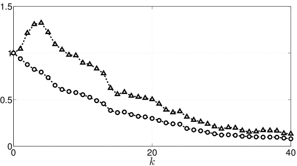
Figure 1: The sample means of the Lyapunov function (circle) and the Euclidean norm (triangle)

Figure 1 shows the sample means of the stochastic Lyapunov function $\lVert{x(k)}\rVert_{f}$ and the Euclidean norm $\lVert{x(k)}\rVert$. We can see that the sample mean of the Lyapunov function decreases at the most of time instances, while that of the Euclidean norm shows an oscillating behavior. It is remarked that the sample mean of the Lyapunov function is not necessarily decreasing because it is actually different from the expectation. Taking more sample paths in general makes the sample mean closer to the expectation by the law of large numbers and therefore is more likely to yield a decreasing sample mean.

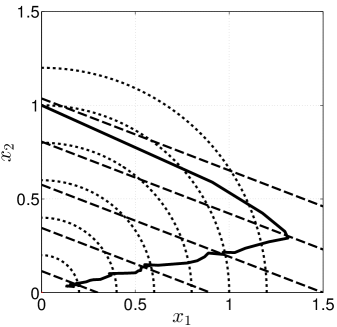
Figure 2: The averaged sample path (solid) and the level plots of the Lyapunov function (dashed) and the Euclidean norm (dotted)

Figure 2 shows the average of the sample paths and the contour plot of the stochastic Lyapunov function and the Euclidean norm. The figure graphically illustrates that the sample mean is evolving in such a way that the value of constructed Lyapunov function almost decreases.

6 Conclusion and Discussion

This paper presented a characterization of the joint spectral radius of a set of matrices as the limit of the $L^{p}$-norm joint spectral radius of a probability distribution on the set when $p\to\infty$ under the assumption that the distribution has a certain regularity and a support leaving a proper cone invariant. The obtained characterization extends the ones in the literature by allowing the set to have infinitely many matrices. Based on the result, we also presented a novel characterization of the absolute exponential stability of switched linear systems via the existence of stochastic Lyapunov functions of any higher degrees. The construction of stochastic Lyapunov functions is also studied.

Understanding the behavior of $p$-radius as $p\to 0$ is one of the problems closely related to the problem studied in this paper. It is known [33] that, as $p\to 0$, the $p$-radius converges to so-called Lyapunov exponent [34] of random products of matrices, which is known to characterize so-called almost sure stability of stochastic switched systems. However the characterization in [33] is proved under the assumption that the number of matrices in the set from which one takes a matrix is finite. It would be interesting to investigate if one can allow the number of matrices to be infinite with the approach taken in this paper.

References

- Rota and Strang [1960] G.-C. Rota, W. G. Strang, A note on the joint spectral radius, Indag. Math 22 (1960) 379–381.
- Jungers [2009] R. M. Jungers, The Joint Spectral Radius, volume 385 of Lecture Notes in Control and Information Sciences, Springer Berlin Heidelberg, Berlin, Heidelberg, 2009.
- Tsitsiklis and Blondel [1997] J. N. Tsitsiklis, V. D. Blondel, The Lyapunov exponent and joint spectral radius of pairs of matrices are hard – when not impossible – to compute and to approximate, Mathematics of Control, Signals, and Systems 10 (1997) 31–40.
- Blondel and Nesterov [2005] V. D. Blondel, Y. Nesterov, Computationally efficient approximations of the joint spectral radius, SIAM Journal on Matrix Analysis and Applications 27 (2005) 256–272.
- P. A. Parrilo and Jadbabaie [2008] P. A. Parrilo, A. Jadbabaie, Approximation of the joint spectral radius using sum of squares, Linear Algebra and its Applications 428 (2008) 2385–2402.
- Protasov et al. [2010] V. Y. Protasov, R. M. Jungers, V. D. Blondel, Joint spectral characteristics of matrices: a conic programming approach, SIAM Journal on Matrix Analysis and Applications 31 (2010) 2146–2162.
- Vankeerberghen et al. [2014] G. Vankeerberghen, J. Hendrickx, R. M. Jungers, JSR: A toolbox to compute the joint spectral radius, in: Proceedings of the 17th international conference on Hybrid systems: computation and control, pp. 151–156.
- Jia [1995] R.-Q. Jia, Subdivision schemes in spaces, Advances in Computational Mathematics 3 (1995) 309–341.
- Wang [1996] Y. Wang, Two-scale dilation equations and the mean spectral radius, Random and Computational Dynamics 4 (1996) 49–72.
- Protasov [1997] V. Y. Protasov, The generalized joint spectral radius. A geometric approach, Izvestiya: Mathematics 61 (1997) 995–1030.
- Jungers and Protasov [2011] R. M. Jungers, V. Y. Protasov, Fast methods for computing the -radius of matrices, SIAM Journal on Scientific Computing 33 (2011) 1246–1266.
- Jungers and Protasov [2010] R. M. Jungers, V. Y. Protasov, Weak stability of switching dynamical systems and fast computation of the -radius of matrices, in: 49th IEEE Conference on Decision and Control, pp. 7328–7333.
- Ogura and Martin [2013a] M. Ogura, C. F. Martin, Generalized joint spectral radius and stability of switching systems, Linear Algebra and its Applications 439 (2013a) 2222–2239.
- Ogura and Martin [2013b] M. Ogura, C. F. Martin, On the mean stability of a class of switched linear systems, in: 52nd IEEE Conference on Decision and Control, pp. 97–102.
- Lin and Antsaklis [2009] H. Lin, P. Antsaklis, Stability and stabilizability of switched linear systems: a survey of recent results, IEEE Transactions on Automatic Control 54 (2009) 308–322.
- Shorten et al. [2007] R. Shorten, F. Wirth, O. Mason, K. Wulff, C. King, Stability criteria for switched and hybrid systems, SIAM Review 49 (2007) 545–592.
- Seidman et al. [2005] T. I. Seidman, H. Schneider, M. Arav, Comparison theorems using general cones for norms of iteration matrices, Linear Algebra and its Applications 399 (2005) 169–186.
- Bertram and Sarachik [1959] J. Bertram, P. Sarachik, Stability of circuits with randomly time-varying parameters, IRE Transactions on Circuit Theory 6 (1959) 260–270.
- Ahmadi [1979] G. Ahmadi, On the mean square stability of linear difference equations, Applied Mathematics and Computation 241 (1979) 233–241.
- Feng et al. [1992] X. Feng, K. A. Loparo, Y. Ji, H. J. Chizeck, Stochastic stability properties of jump linear systems, IEEE Transactions on Automatic Control 31 (1992) 38–53.
- Dayawansa and Martin [1999] W. Dayawansa, C. Martin, A converse Lyapunov theorem for a class of dynamical systems which undergo switching, IEEE Transactions on Automatic Control 44 (1999) 751–760.
- Molchanov and Pyatnitskiy [1989] A. Molchanov, Y. Pyatnitskiy, Criteria of asymptotic stability of differential and difference inclusions encountered in control theory, Systems & Control Letters 13 (1989) 59–64.
- Lang [1986] R. Lang, A note on the measurability of convex sets, Archiv der Mathematik 47 (1986) 90–92.
- Berman and Plemmons [1979] A. Berman, R. J. Plemmons, Nonnegative Matrices in the Mathematical Sciences, SIAM, Philadelphia, 1979.
- Brewer [1978] J. Brewer, Kronecker products and matrix calculus in system theory, IEEE Transactions on Circuits and Systems 25 (1978) 772–781.
- Bogachev [2007] V. I. Bogachev, Measure Theory, Springer Berlin Heidelberg, Berlin, Heidelberg, 2007.
- Gurvits [1995] L. Gurvits, Stability of discrete linear inclusion, Linear Algebra and its Applications 231 (1995) 47–85.
- Wirth [2002] F. Wirth, The generalized spectral radius and extremal norms, Linear Algebra and its Applications 342 (2002) 17–40.
- Xu and Xiao [2011] J. Xu, M. Xiao, A characterization of the generalized spectral radius with Kronecker powers, Automatica 47 (2011) 1530–1533.
- Ando and Shih [1998] T. Ando, M.-H. Shih, Simultaneous contractibility, SIAM Journal on Matrix Analysis and Applications 19 (1998) 487–498.
- Protasov [2008] V. Y. Protasov, Extremal -norms of linear operators and self-similar functions, Linear Algebra and its Applications 428 (2008) 2339–2356.
- Vandergraft [1968] J. S. Vandergraft, Spectral properties of matrices which have invariant cones, SIAM Journal on Applied Mathematics 16 (1968) 1208–1222.
- Fang and Loparo [2002] Y. Fang, K. A. Loparo, On the relationship between the sample path and moment Lyapunov exponents for jump linear systems, IEEE Transactions on Automatic Control 47 (2002) 1556–1560.
- Arnold [1984] L. Arnold, A formula connecting sample and moment stability of linear stochastic systems, SIAM Journal on Applied Mathematics 44 (1984) 793–802.