Empirical geodesic graphs and CAT(k) metrics for data analysis

Abstract.

A methodology is developed for data analysis based on empirically constructed geodesic metric spaces. For a probability distribution, the length along a path between two points can be defined as the amount of probability mass accumulated along the path. The geodesic, then, is the shortest such path and defines a geodesic metric. Such metrics are transformed in a number of ways to produce parametrised families of geodesic metric spaces, empirical versions of which allow computation of intrinsic means and associated measures of dispersion. These reveal properties of the data, based on geometry, such as those that are difficult to see from the raw Euclidean distances. Examples of application include clustering and classification. For certain parameter ranges, the spaces become CAT(0) spaces and the intrinsic means are unique. In one case, a minimal spanning tree of a graph based on the data becomes CAT(0). In another, a so-called “metric cone” construction allows extension to CAT($k$) spaces. It is shown how to empirically tune the parameters of the metrics, making it possible to apply them to a number of real cases.

1. Introduction

In much statistics and data analysis, the metric (distance) for data points is fixed and the loss function is selected from a set of candidates for loss functions and/or tuned by a parameter. However, in the paper, we fix a loss function (usually the squared loss) and instead select/tune the metric. The motivation of such metric-based approach is to propose a set of metrics and a method to select a metric from it which are naturally acquired from geometrical aspects. This enables us to import huge existing literature of various branches of geometry into data analysis. We will begin by focusing the curvature. In this section, after explanation by a motivational example, exiting studies related to our geometrical approach will be surveyed.

1.1. Example

For a random variable $X$ on a metric space $\mathcal{M}$ endowed with a metric $d(\cdot,\cdot)$ the general intrinsic mean is defined by

$$\mu=\mbox{arg}\min_{m\in\mathcal{M}}\mbox{E}[d(X,m)^{2}].$$

The empirical intrinsic mean based on data $x=\{x_{1},\ldots,x_{n}\}$, sometimes called the Fréchet mean, is defined as

$$\hat{\mu}=\mbox{arg}\min_{m\in\mathcal{M}}f(m),$$

where

$$f(m)=\sum_{i=1}^{n}d(x_{i},m)^{2}.$$

The function $f(m)$ is sometimes referred to as the Fréchet function. For Euclidean space, $\hat{\mu}=\bar{x}$, the sample mean. In general, $f(m)$ is not necessarily convex and the means, $\hat{\mu}$, are not unique. Figure 1 shows that the curvature can affect the property of $f(m)$. In particular, for so-called CAT(0) spaces, which (trivially) include Euclidean spaces, the intrinsic means $\hat{\mu}$ are unique.

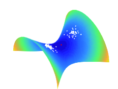
(a) Hyperboloid

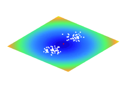
(b) Plane

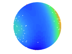
(c) Sphere

Figure 1. The Fréchet function $f(m)$ for data (white dots) on (a) a hyperboloid (curvature $c=-1$), (b) a plane ($c=0$) and (c) a sphere ($c=1$). The bluer represents the smaller value of $f(m)$. The red dots represent the local minima of $f(m)$. Only for the sphere, $f(m)$ has multiple minima.

Even when the mean is not unique, the function $f(m)$ can yield useful information, for example about clustering. We can also define second-order quantities:

$$s_{0}^{2}=\inf_{m\in\mathcal{M}}\frac{1}{n}\sum_{i=1}^{n}d(x_{i},m)^{2}=\frac{1}{n}\sum_{i=1}^{n}d(x_{i},\hat{\mu})^{2}$$

and

$$s_{1}^{2}=\frac{2}{n(n-1)}\sum_{i<j}^{n}d(x_{i},x_{j})^{2}.$$

The quantity $s_{0}^{2}$ is sometimes called the Fréchet variance. We name $s_{1}^{2}$ as the mean pairwise discrepancy.

A key concept in the study of these issues is that the metrics are global geodesic metrics, that is metrics based on the shortest path between points measured by integration along a path with respect to a local metric. The interplay between the global and the local will concern us to a considerable extent.

The general form of the Fréchet function depends, here, on three parameters, $\alpha,\beta,\gamma,$ and it can be written in compact form:

$$f_{\alpha,\beta,\gamma}(m)=\sum_{i=1}^{n}\{g_{\beta}(d_{\alpha}(x_{i},m))\}^{\gamma},$$

where the function $g_{\beta}$ and the construction of $d_{\alpha}$ are given below. Once we have introduced this new class of metrics, variety of statistics can be generalised: intrinsic mean, variance, clustering (based on local minima of $f(m)$). For classification problems, we can select an appropriate metric by cross-validation.

There are many ways to transform one metric into another, regardless of whether they are geodesic metrics. A straightforward way is to use a concave function $g$ such that given a metric $d(\cdot,\cdot)$, the new metric is $d^{\prime}(\cdot,\cdot)=g(d(\cdot,\cdot))$. This is plausible if we use non-convex $f_{\alpha,\beta,\gamma}$, which are useful, as will be explained, in clustering and classification. Such concave maps are often interpreted as loss functions, but we will consider them in terms of changes of metric which may lead to selection using geometric concepts. This is particularly true for the construction based on the $g_{\beta}$ in Section 3 of the paper. In Table 1, we summarise such generalised statistics.

Table 1. A summary of generalised statistics by introducing $\alpha,\beta$ and $\gamma$.

	Euclidean	Generalised metric
Metrics	$d(x,y)=\|x-y\|$	$d_{\alpha\beta}(x,y)=g_{\beta}(d_{\alpha}(x,y))$
Intrinsic mean	$\displaystyle\arg\min_{m\in\mathbb{E}^{d}}\sum_{i=1}^{n}\|x_{i}-m\|^{2}$	$\displaystyle\arg\min_{m\in\mathcal{M}}\sum_{i=1}^{n}g_{\beta}(d_{\alpha}(x_{i},m))^{\gamma}$
Variance	$\displaystyle\min_{m\in\mathbb{E}^{d}}\frac{1}{n}\sum_{i=1}^{n}\|x_{i}-m\|^{2}$	$\displaystyle\min_{m\in\mathcal{M}}\frac{1}{n}\sum_{i=1}^{n}g_{\beta}(d_{\alpha}(x_{i},m))^{\gamma}$
Fréchet function	$f(m)=\displaystyle\sum_{i=1}^{n}\|x_{i}-m\|^{2}$	$f_{\alpha\beta\gamma}(m)=\displaystyle\sum_{i=1}^{n}g_{\beta}(d_{\alpha}(x_{i},m))^{\gamma}$

The basic definition and construction from a geodesic metric space to the special geodesics based on accumulation of density are given in the next section, together with the definition of a CAT(0) space. In Section 2, we first show that means and medians in simple one-dimensional statistics can be placed into our framework. Because geodesics themselves are one-dimensional paths, this should provide some essential motivation. The $d_{\alpha}$-metric is obtained by a local dilation. Our computational shortcut is to use empirical graphs, whose vertices are data points.

We will need, therefore, to define empirical geodesics. We start with a natural geodesic defined via a probability density function in which the distance along a path is the amount of density “accumulated” along that path. Then, an empirical version is defined whenever a density is estimated.

In Section 4, the $d_{\beta}$ metric is introduced. It is based on a function derived from a geodesic metric via shrinking, pointwise, to an abstract origin (apex); that is to say an abstract cone is attached. The smaller the value of $\beta$, the closer to the origin. We cover the more general CAT($k$) spaces, giving some new results related to “diameter” , in Section 5, including conditions for the uniqueness of intrinsic means not requiring the spaces to be CAT(0).

Section 6 provides a summary of the effect of changing $\alpha$ and $\beta$. After some discussion of the selection of $\alpha$ and $\beta$ in Section 7, Section 8 covers some examples.

1.2. Related existing studies

Manifold learning is a group of nonlinear dimension reduction techniques including well-studied methods such as Isomap (Tenenbaum et al (2000)), Locally Linear Embedding (LLE) (Saul (2003)) and Laplacian Eigenmaps (Belkin and Niyogi (2002)). Most manifold learning methods are based on the “manifold hypothesis,” which is an assumption that the data is distributed around a smooth manifold with a lower dimension embedded in a higher-dimensional vector space (usually Euclidean space). There are some similarity between the methods proposed in this paper and manifold learning methods though the original motivation of the research is different; both methods focus on the geometrical structure of an embedded data space and, furthermore, use the geodesic length (shortest path length) in an empirical graph as the distance between data points. Our methods have significant differences from the manifold learning methods. First, we control the curvature of the data space for data analysis via changing the metric while the metric in manifold learning context is fixed and to be estimated. Second, sometimes more positively (or negatively) curved data space is preferable in contrast to a situation in most manifold learning methods which attempt to estimate the manifold by making the approximated empirical graph locally flat (Euclidean) as possible. For more details of the manifold learning methods, there are good surveys, e.g. Yang and Jin (2006), Cayton (2005) (with other metric learning methods such as kernel learning) and Bengio et al (2013)(with various other data representation for machine learning).

Statistical shape analysis (Kendall et al (2009), Ramsay and Silverman (2007), Srivastava and Klassen (2016)), also known as object oriented data analysis (Marron and Alonso (2014)), has a long history after a pioneering work by Kendall (1984) on random segmentations. Statistical shape analysis studies geometrical structure of the set (shape space) of possible populations which themselves have some particular shapes. For various kinds of shape spaces, computation of center points as mean and median and statistical methods as PCA and Bootstrap tests have been studied (see, e.g. Dryden and Mardia (2016)). In particular, Tree space for analyzing phylogenetic trees (Billera et al (2001), Wang and Marron (2007)) is closely related to our research. Tree space is a set of tree graphs and the set is embedded in a Euclidean space with a tacitly defined metric. The space is proved to have the CAT(0) property and therefore both geodesics between any pair of points and Fréchet mean of any finite data sets exit uniquely. Furthermore, a polynomial algorithm to compute the geodesics (Owen and Provan (2011)) and PCA on Tree space (Nye (2011)) have been proposed. Besides such non-smooth spaces as Tree space, there have been many studies of non-parametric statistics on smooth manifolds. There are excellent textbooks in this area such as Bhattacharya and Bhattacharya (2012a), Patrangenaru and Ellingson (2015).

Data analysis using Wasserstein distance also focuses geodesic distance in the space of probability measures (see, e.g., Vallender (1974), Villani (2008), Peyré and Cuturi (2018)). Wasserstein Fréchet mean of measures is also studied (Cuturi and Doucet (2014)) and uniqueness and computation of the mean depends on the curvature of the Wasserstein space. For example, the 2-Wasserstein space for Gaussian measures has positive curvature in general (Takatsu (2011)) and therefore computation of Wasserstein Fréchet mean is difficult. Panaretos and Zemel (2018) is a useful survey of Wasserstein metric from statistical aspects and geometry of Wasserstein space is summarized in a section. Because most of the recent algorithms in machine learning and computer graphics are based on some gradient methods, Wasserstein metric is becoming an active topic in such areas, e.g. Wasserstein-GAN (Arjovsky et al (2017)) and optimal transport of graphics with a penalty on the entropy (Solomon et al (2015)).

Another area in statistics directly dealing with the curvatures is information geometry (Amari (1985), McCullagh (1986)). Fisher metric, based on the Fisher information matrix, is induced in a statistical model manifold which is curved in an embedding space (usually flat, for example, the space of an exponential family). The asymptotic property and efficiency of estimators and predictors can be represented by the embedding curvature and naturally induced dual affine connections. The role of curvatures in information geometry can be somewhat negative; even if the model manifold has non-zero embedding curvature, still some asymptotic efficiency of estimators (like bias-corrected MLE) can be proved.

As we have explained, there are many studies on statistics and data analysis using geodesics and curvatures, but our methods have some special features:

• The curvature of the data space holds not only by its own nature, but is controlled for data analysis.

• The structure of empirical graphs used for computing the distance between the data points is not fixed but transformed via controlling the curvature.

• Our methods can produce non-geodesic distances for data analysis from the aspects of curvatures though the curvatures cannot be defined for non-geodesic metric spaces. This was achieved by considering the curvature of a metric space embedding the data space.

2. Geodesics, intrinsic mean and extrinsic mean

The fundamental object in this paper is a geodesic metric space. This is defined in two stages. First, define a metric space $\mathcal{M}=(X,d)$ with base space $X$ and metric $d(x,x^{\prime})$. Sometimes, $\mathcal{M}$ will be a Euclidean space $E_{d}$ of dimension $d$, containing the data points, but it may also be some special object such as a graph or manifold. Second, define the length of a (rectilinear) path between two points $x,x^{\prime}\in X$ and the geodesic connecting $x$ and $x^{\prime}$ as the shortest such path. The minimal length defines a metric $d^{*}(x,x^{\prime})$, and the space endowed with the geodesic metric is called the geodesic metric space, $\mathcal{M}^{*}={\mathcal{M}}(X,d^{*})$.

The interplay between $\mathcal{M}=(X,d)$ and $\mathcal{M}^{*}=(X,d^{*})$ will be critical for this paper, and, as mentioned, we will have a number of ways of constructing $d^{*}$.

For data points $x_{1},\ldots,x_{n}$ in $X$, the empirical intrinsic (Fréchet) mean is

$$\mu=\arg\inf_{\mu\in X}\sum_{i=1}^{n}d^{*}(x_{i},\mu)^{2}.$$

There are occasions when ${\mathcal{M}}^{*}$ can be represented as a sub-manifold of a larger space (such as Euclidean space) ${\mathcal{M}}^{+}=(X^{+},d^{+})$ with its own metric $d^{+}$. We can then talk about the extrinsic mean:

$$\mu^{+}=\arg\inf_{\mu\in X}\sum_{i=1}^{n}d^{+}(x_{i},\mu)^{2}.$$

Typically, the extrinsic mean is used as an alternative when the geodesic distance $d^{*}$ is hard to compute. The difficultly in considering the intrinsic mean in $X^{+}$ is that it may not lie in the original base space $X$. This leads to a third possibility, which is to project it back to $X$, in some way, as an approximation to the intrinsic mean $\mu$ (which may be hard to compute). We will discuss this again in Section 4. See Bhattacharya and Bhattacharya (2012b) for further discussion on the intrinsic and extrinsic means.

2.1. CAT(0) and CAT($k$) spaces

CAT(0) spaces, which correspond to non-positive curvature Riemannian spaces, are important here because their intrinsic means are unique. The CAT(0) property is as follows. Take any three points $\{a,b,c\}$ in a geodesic metric space $X$ and consider the “geodesic triangle” of the points based on the geodesic segments connecting them. Construct a triangle in Euclidean 2-space with vertices $\{a^{\prime},b^{\prime},c^{\prime}\}$, called the comparison triangle, whose Euclidean distances, $\|a^{\prime}-b^{\prime}\|,\|b^{\prime}-c^{\prime}\|,\|a^{\prime}-c^{\prime}\|$, are the same as the corresponding geodesic distances just described: $d(a,b)=\|a^{\prime}-b^{\prime}\|$, etc. On the geodesic triangle select a point $x$ on the geodesic edge between $b$ and $c$ and find the point $x^{\prime}$ on the edge $b^{\prime}c^{\prime}$ of the Euclidean triangle such that $d(b,x)=\|b^{\prime}-x^{\prime}\|$. Then the CAT(0) condition is that for all $a,b,c$ and all choices of $x$:

(1) $$d(x,a)\leq\|x^{\prime}-a^{\prime}\|.$$

For a CAT(0) space (i) there is a unique geodesic between any two points, (ii) the space is contractible, in the topological sense, to a point and (iii) the intrinsic mean in terms of the geodesic distance is unique. See Gromov (1987) for properties of CAT(0).

Next consider CAT($k$) space which in essence generalizes CAT(0) space. Consider a geodesic triangle $abc$ whose perimeter is less than $2\pi/\sqrt{\max(k,0)}$ for $k\in\mathbb{R}$ and a comparison triangle $a^{\prime}b^{\prime}c^{\prime}$ on a surface $\mathcal{M}_{k}$ with a constant curvature $k$. If the inequality (1) holds for $x$ and $x^{\prime}$ selected in the same manner but with the geodesic length $d_{\mathcal{}M_{k}}(x^{\prime},a^{\prime})$ on the surface $\mathcal{M}_{k}$ is used instead of the Euclidean distance $\|x^{\prime}-a^{\prime}\|$, we say the geodesic metric space has CAT($k$) property. Thus every CAT($k$) space is a CAT($k^{\prime}$) space for $k<k^{\prime}$. Intuitively speaking, CAT(0) space is a space with non-positive sectional curvatures and CAT($k$) space is a space with sectional curvatures at most $k$. See, for example, Bridson and Haefliger (2011) for detailed explanation of CAT(0) and CAT($k$) spaces.

2.2. Geodesic metrics on distributions

Let $X$ be a $d$-dimensional Euclidean random variable absolutely continuous with respect to the Lebesgue measure, with density $f(x)$. Let $\Gamma=\{z(t),t\in[0,1]\}$ be a parametrised integrable path between two points $x_{0}=z(0),x_{1}=z(1)$ in $\mathbb{R}^{d}$, which is rectifiable with respect to the Lebesgue measure. Let

$$s(t)=\sqrt{\sum_{i=1}^{d}\left(\frac{\partial z_{i}(t)}{\partial t}\right)^{2}},$$

with appropriate modification in the non-differentiable case, be the local element of length along $\Gamma$. The weighted distance along $\Gamma$ is

(2) $$d_{\Gamma}(x_{0},x_{1})=\int_{0}^{1}s(t)f(z(t))dt$$

The geodesic distance is

$$d(x_{0},x_{1})=\inf_{\Gamma}d_{\Gamma}(x_{0},x_{1}).$$

Here we consider a random variable on Euclidean space but this can be generalized for Riemannian manifolds and even for singular spaces with a density with respect to a base measure naturally defined by the metric.

From the geodesic distances on distributions we shall follow three main directions:

1. transform the geodesic metrics in various ways with parameters $\alpha,\beta$ to obtain a wide class of metrics,

2. discover (locally) CAT(0) and CAT($k$) spaces for certain ranges of the parameters,

3. apply empirical versions of the metrics based on an empirical graph whose nodes are the data points.

There is an important distinction between global transformations applied to the whole distance between points and local transformations applied to dilate the distance element.

3. The $d_{\alpha}$ metric and the geodesic subgraphs

The general $d_{\alpha}$ metric is a dilation of the original distance $d$ and what we have referred to as a local metric. It is obtained by transforming the density in (2). Thus for $\Gamma=\{z(t),t\in[0,1]\}$ between $x_{0}=z(0)$ and $x_{1}=z(1)$,

$$d_{\Gamma,\alpha}(x_{0},x_{1})=\int^{1}_{0}s(t)f^{\alpha}(z(t))dt$$

and

$$d_{\alpha}(x_{0},x_{1})=\inf_{\Gamma}d_{\Gamma,\alpha}(x_{0},x_{1}).$$

Here $\alpha$ is any real number. Changing $\alpha$ essentially changes the local curvature. Roughly speaking, when $\alpha$ is more negative (positive), the curvature is more negative (positive). In section 6.1, we will explain how to select the value of $\alpha$ for data analysis. Values between -5 to 1 are usually selected.

In the next subsection, we look at the one-dimensional case. Although this case is elementary, good intuition is obtained by rewriting the standard version in terms of a geodesic metric.

3.1. One-dimensional means and medians

Assume that $X$ is a continuous univariate random variable with probability density function $f(x)$ and cumulative distribution function (CDF) $F(x)$. The mean $\mu=\makebox{E}[X]$ achieves $\displaystyle\min_{m}\makebox{E}[(X-m)^{2}]$. Here we are using the Euclidean distance: $d_{E}(x,y)=|x-y|$.

The median is defined by $\nu=F^{-1}(1/2)$. On a geometric basis, we can say that $\nu$ achieves $\displaystyle\min_{m}E_{X}[d_{D}(m,X)^{2}]$, where we use a metric that measures the amount of probability between $x$ and $z$:

(3) $$d_{D}(x,z)=|F(x)-F(z)|.$$

Carrying out the calculations:

$$\mbox{E}_{X}[d_{D}(m,X)^{2}] =\int_{-\infty}^{\infty}(F(m)-F(x))^{2}f_{X}(x)dx$$

$$=\frac{1}{3}-F(m)(1-F(m))$$

which achieves a minimum of $\frac{1}{12}$ at $F(m)=\frac{1}{2}$, as expected.

Another approach for the median would be to take a piecewise linear approximation to $F$ which is equivalent to having a density $\hat{f}$ that is proportional to $\frac{1}{x_{(n+1)}-x_{(n)}}$ in the interval $[x_{(n)},x_{(n+1)})$. Then, the metric is

$$\tilde{d}_{2}(x,z)=\int_{\min(x,z)}^{\max(x,z)}\hat{f}(y)dy,$$

and $\displaystyle\min_{m}\sum_{i=1}^{n}\tilde{d}_{2}(x_{i},m)^{2}$ is achieved at $x_{(\frac{n+1}{2})}$ when $n$ is odd and at $\frac{1}{2}(x_{(\frac{n}{2})}+x_{(\frac{n+2}{2})})$, when $n$ is even.

The idea of weighting intervals should provide intuition when we extend the intervals to edges on a graph, because edges are one-dimensional.

3.2. The $d_{\alpha}$ metric for graphs

There are a number of options to define an empirical version of the $d_{\alpha}$ metric, based on data. One such option would be to produce a smooth empirical density $f(t)$ followed by numerical integration and optimization to compute the geodesics. We prefer a much simpler method based on a metric graph whose vertices are the data points. All geodesic computation is then restricted to the graph. We list some candidates: (1) the complete graph, (2) the edge graph (1-skeleton) of the Delaunay simplicial complex, (3) the Gabriel graph, (4) the $k$-NN graph, etc. (see, for example, Okabe et al (2009) for Delaunay complex and Gabriel graph). The discussion below applies to the complete graph or any connected sub-graph.

For any such graph, define a version of the $d_{\alpha}$ distance just for edges,

$$\tilde{d}_{\alpha,ij}=d_{ij}^{1-\alpha},$$

where $d_{ij}$ is the Euclidean distance from $x_{i}$ to $x_{j}$. This can be explained by making a transformation $ds\rightarrow\frac{ds}{d_{ij}}.$ We refer to this as edge regularization. We then apply $\alpha$ in the usual way to obtain $\frac{ds}{d_{ij}^{\alpha}}.$ The new “length” of each edge $e_{ij}$ is obtained by integrating this “density” along the edge. In this sense, $d_{ij}$ also plays the role of density estimation. Although we need a regularization $d_{ij}^{-1/p}$ with respect to the dimension $p$ for density estimation (see Kendall and Morán (1963)), we manage the regularization by rescaling the parameter $\alpha$. Note that $\alpha=1$ gives the unit length and $\alpha=0$ restores the original length.

Now we consider only the set of edges $E$ of the graph $G(V,E)$ as a metric space with the metric defined by the geodesic:

$$\tilde{d}_{\alpha}(x_{0},x_{1})=\inf_{\Gamma}\sum_{(i,j)\in\Gamma}\tilde{d}_{\alpha,ij},$$

where the infimum is taken over all (connected) paths $\Gamma$ between $x_{0}$ and $x_{1}$. Here we will admit $\tilde{d}_{\alpha}$ as an approximation of $d_{\alpha}$.

Note that the graph is not a complete Euclidean graph with weights equal to the Euclidean lengths of the edges, some edges may not be in any edge geodesics between any pair of vertices.

Definition 3.1.

For an edge-weighted graph $G$ with weights $\{d_{ij}\}$ on the graph, $G^{*}$, which is the union of all the edge geodesics between all pairs of vertices, is called the geodesic sub-graph (or geodesic graph) of $G$.

We will see how the geodesic sub-graphs transform as the value of $\alpha$ changes.

We make an important general position assumption that the set of values $\{d_{ij}\mid(i,j)\in E\}$ are distinct, that is there are no ties. We order the values using only a single suffix for simplicity: $d_{1}<d_{2}<\cdots<d_{M}$ where $M=|E|$. For $\alpha<1$, this induces the $\tilde{d}_{\alpha,i}(=d_{i}^{1-\alpha})$ values:

$$\tilde{d}_{\alpha,1}<\tilde{d}_{\alpha,2}<\cdots<\tilde{d}_{\alpha,M}.$$

Now, consider the geodesics as $\alpha\rightarrow-\infty$. Recall that a circuit in a graph is a connected path that begins and ends in some vertex and an elementary circuit is a circuit that visits a vertex no more than once. Consider an edge $(i,j)\in E$ that has the following property which we call $Q$: it is in an elementary circuit $\mathcal{C}$ of the graph in which all other edges have smaller values of $d_{ij}$ namely

$$d_{rs}<d_{ij}\mbox{ for }(r,s)\in\mathcal{C},\;(r,s)\neq(i,j).$$

Then, the path $\Gamma(i,j)$ (within the circuit) from $x_{i}$ to $x_{j}$ not containing the edge $(i,j)$ has length smaller than $\tilde{d}_{\alpha,ij}$ when $\alpha$ is sufficiently negative:

$$\sum_{(r,s)\in\Gamma(i,j)}d_{rs}^{1-\alpha}<d_{ij}^{1-\alpha}$$

From this argument, we see that for sufficiently large $|\alpha|$ as $\alpha$ approaches $-\infty$, every edge having property Q is removed from the geodesic sub-graph, and we obtain a tree.

Let us summarize this algorithm, which applies to a general edge-weighted graph with distinct edges. We refer to this algorithm as the backwards algorithm. It clearly gives a tree.

1. Let $|E|=M$ and label the edges $e_{1},\ldots,e_{M}$ in increasing order of their weights.

2. Starting with edge $e_{M}$, remove $e_{M}$ if it is in a cycle otherwise continue to $e_{M-1}$.

3. (General step) Continue downwards at each stage removing an edge if it is in a cycle of the remaining subgraph.

4. Stop if no more edges can be removed using step 3.

There is a natural forwards algorithm that also yields a tree as follows.

1. Let $|E|=M$ and label the edges $e_{1},\ldots,e_{M}$ in increasing order of their weights.

2. Starting with $e_{1}$, add an edge if adding it does not create a cycle.

3. (General step) Continue adding an edge at each step provided that the addition does not create a cycle.

4. Stop if no more edges can be added.

We have the following theorem (the proof is in the appendix).

Theorem 3.2.

Given a connected edge-weighted graph $G(V,E)$ with distinct edge weights $\{d_{ij},\;(i,j)\in E\}$, the backward and forward algorithms yield the same tree, which we call $T^{*}(G)$. Furthermore, $T^{*}(G)$ becomes the minimum spanning tree of $G$.

For sufficiently negative $\alpha$, the tree $T$ itself, that is the tree as a metric space with metric $d_{\alpha}$, is a CAT(0) space (Deza and Deza (2009)). We need to extend the metric somewhat so that it applies to the edges, in addition to the nodes. Thus, for any two points $x,x^{\prime}$ on the tree, define

$$d_{\alpha}(x,x^{\prime})=\inf_{\Gamma(x,x^{\prime})}\int_{\Gamma(x,x^{\prime})}w(s)ds,$$

where the integral is taken along the (unique) path $\Gamma(x,x^{\prime})$ on the tree and $w(s)=\frac{1}{d_{ij}^{\alpha}}$ when line element $ds$ is in edge $e$ in $\Gamma(x,x^{\prime})$. Since every metric tree is a CAT(0) space, the following is an immediate consequence of Theorem 3.2.

Corollary 3.3.

There is an $\alpha^{*}$ such that for any $\alpha\leq\alpha^{*}$, the geodesic sub-graph becomes the minimal spanning tree $T^{*}(G)$ endowed with the $d_{\alpha}$ metric and, therefore, becomes a CAT(0) space.

We see that for sufficiently negative $\alpha$, every geodesic defined with the $d_{\alpha}$ metric lies in the tree $T^{*}$. In fact, although we started with a general connected graph, any graph for which the edges can be mapped into a Euclidean interval gives a CAT(0) tree using this construction.

Furthermore, the geodesic subgraph “shrinks” as $\alpha$ changes away from 1.

Theorem 3.4.

Let $G_{\alpha}$ be an edge-weighted graph with distinct weights $\{d_{ij}^{1-\alpha}\}$ and let $G^{*}_{\alpha}$ be its geodesic subgraph; then for any real $\alpha$ and $\alpha^{\prime}$,

$$|1-\alpha^{\prime}|>|1-\alpha|\Rightarrow G^{*}_{\alpha^{\prime}}\subseteq G^{*}_{\alpha}.$$

Here $\subseteq$ represents the inclusion of the edge sets.

Proof. This follows from the consideration of geodesics. An edge $(i,j)$ in $G$ is not in $G^{*}_{\alpha}$ if it is not a geodesic. In this case, there is an alternative path $\Gamma$ from $i$ to $j$ such that $d_{ij}^{1-\alpha}>\sum_{(r,s)\in\Gamma}d_{rs}^{1-\alpha}$. However, this inequality is preserved if $\alpha$ is decreased, so that $1-\alpha$ is increased. Thus an edge absent from $G^{*}_{\alpha}$ is absent from $G^{*}_{\alpha^{\prime}}$. ∎

Note that, while Theorem 3.4 holds for any real $\alpha$ and $\alpha^{\prime}$, in application $\alpha$ is usually set at most one since otherwise the ordering of the magnitude of $d_{ij}$s becomes the inverse by taking the $1-\alpha$-th power.

3.3. $\alpha$ and CAT($k$)

If a space is CAT(0), then it is CAT($k$) for all $k>0$. Let $C(X,p,r):=\{x\in X\mid d(p,x)\leq r\}$ be a geodesic disk of radius $r\geq 0$ centred at $p\in X$. Define the maximum radius $D_{k}(X,x)$ of the disk centred at $x$ as being CAT($k$), that is

$$D_{k}(X,x):=\sup\{r\geq 0\mid X\cap C(X,x,r)~{}\mbox{is CAT($k$)}\}.$$

If $X$ is a metric graph, $D_{k}(X,x)$ is the maximum radius of the disk which is centred at $x$ and does not include a cycle shorter than $2\pi/\sqrt{\max(k,0)}$.

Consider a rescaling of $X$ such that the shortest (longest) edge length is 1, and denote it as $\bar{X}$ for $\alpha\leq 1$ ($\alpha>1$).

Theorem 3.5.

If $|\alpha^{\prime}-1|>|\alpha-1|$,

$$D_{k}(\bar{G}^{*}_{\alpha^{\prime}},x)>D_{k}(\bar{G}^{*}_{\alpha},x)~{}\mbox{\rm for each}~{}k\in\mathbb{R}.$$

Proof.

Because the $\alpha$-chain is increasing for $\alpha<1$, each cycle in $\bar{G}^{*}_{\alpha}$ is removed one by one as $\alpha$ decreases. Furthermore, each cycle length increases as $\alpha$ decreases because, by the rescaling, every edge length is greater than 1 and it increases as $\alpha$ decreases. This gives the decreasing property of $D_{k}(\bar{G}^{*}_{\alpha},x)$ for $\alpha\leq 1$. We can prove the result for $\alpha>1$ similarly.∎

By the theorem, $\bar{G}^{*}_{\alpha}$ becomes “more CAT($k$)” for a smaller $\alpha<1$. Because rescaling of the graph does not affect the uniqueness of the intrinsic mean, $G^{*}_{\alpha}$ tends to have a unique mean for a smaller $\alpha<1$.

3.4. Geodesic subgraphs in 2-d with different $\alpha$

Figures 2 (a)-(f) are geodesic subgraphs with different values of $\alpha$ for 50 samples of the standard 2-d Normal distribution. We give two cases in which we decrease $\alpha$: the Delaunay graph in Figure 2 and the complete graph in Figure 3. By the time $\alpha=-0.3$ the cases are indistinguishable and have the same minimal spanning geodesic graph for large negative values of $\alpha$, as expected.

This is predictable from Theorem 3.4 and gives an important practical strategy: when the dimension is high and $\alpha$ is small, use the complete graph rather than the Delaunay graph because the former requires computational cost only proportional to $d$, whereas the computational cost of the latter is $O(n^{d/2})$ (see De Berg et al (2000)).

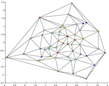
(a) $\alpha=1$

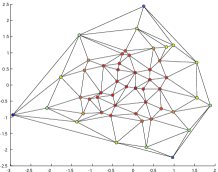
(b) $\alpha=0$

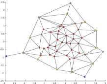
(c) $\alpha=-0.3$

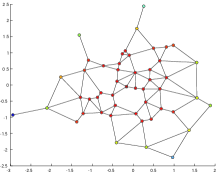
(d) $\alpha=-1$

(e) $\alpha=-5$

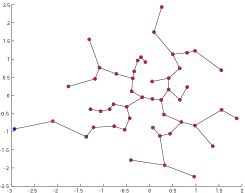
(f) $\alpha=-30$

Figure 2. Geodesic subgraphs with different values of $\alpha$ for 50 samples from the standard 2-d Normal distribution. The initial graph ($\alpha=0$) is the Delaunay graph. The value $f(x)=\sum_{i}d_{\alpha}(x_{i},x)^{2}$ for each sample point $x$ is represented by the colours red (small) and blue (large), and the minimum is represented by a square.

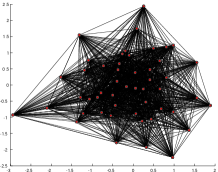
(a) $\alpha=1$

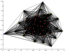
(b) $\alpha=0$

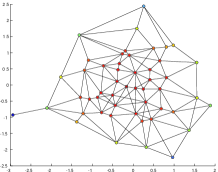
(c) $\alpha=-0.3$

(d) $\alpha=-1$

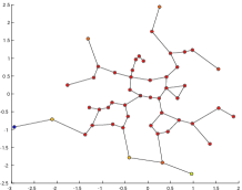
(e) $\alpha=-5$

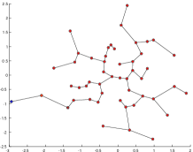
(f) $\alpha=-30$

Figure 3. The figures are made by the same setting of Figure 2 but the initial graph ($\alpha=0$) is the complete graph.

4. The $d_{\beta}$ metric and the metric cones

The CAT(0) property of Euclidean space implies that we do not obtain multiple local minima of the Fréchet function $f$ even for multi-modal distributions. However, an appropriate concave transformation of the metric can modify the base data space making it less CAT(0). We introduce the $d_{\beta}$ metric via a transformation $g_{\beta}$ as a candidate.

For any geodesic metric space $(X,d)$ with metric $d(x_{0},x_{1})$ and a parameter $\beta>0$, we can define the metric

$$d_{\beta}(x_{0},x_{1})=g_{\beta}(d(x_{0},x_{1}))$$

where

$$g_{\beta}(z)=\left\{\begin{array}[]{l}\sin(\frac{\pi z}{2\beta}),\;\mbox{for}\;\;0\leq z\leq\beta,\\ 1,\;\;\mbox{for}\;\;z>\beta.\end{array}\right.$$

Since $g_{\beta}$ is a concave function on $[0,\infty)$, $d_{\beta}$ becomes a metric but not necessarily a geodesic metric. We can express this conveniently as $g_{\beta}(z)=\max\left(\sin(\frac{\pi z}{2\beta}),H(z-\beta)\right)$, where $H$ is the Heaviside function.

It is easiest to consider the case that $d(x_{0},x_{1})$ is the Euclidean distance on the real line. As $\beta\rightarrow\infty$ for small values of $d$, the metric behaves like $\frac{\pi d}{2\beta}$, and as $\beta\rightarrow 0$, it behaves like $\sin(d)$ rescaled to $(0,\beta]$. For Euclidean distances greater than $\beta$, $d_{\beta}$ returns a constant distance of unity. The metric has the effect of downsizing large distances to unity. Because, as will soon be seen, $d_{\beta}$ can be recognized as a geodesic metric of a cone embedding $X$, we refer to the mean

$$\hat{\mu}_{\beta}=\arg\inf_{\mu\in X}\sum_{i=1}^{n}g_{\beta}(d(x_{i},\mu))^{2}$$

as the $\beta$-extrinsic mean.

4.1. The $\beta$-extrinsic mean: one dimension

Controlling $\beta$, as will be seen below, controls the value of $k$ when the embedding space is considered as a CAT($k$) space. We have an indirect link between clustering and CAT($k$) spaces. As $\beta$ decreases while the embedding space becomes more CAT(0) ($k$ decreasing) the original space becomes less CAT(0). This demonstrates, we believe, the importance of the CAT($k$) property in geodesic-based clustering.

In Euclidean space, the standard Euclidean distance dose not exhibit multiple “local means” (i.e. local minimum points of the Fréchet function) because the space is trivially CAT(0). However, by using the $d_{\beta}$-metric with a sufficiently small $\beta$, the space can have multiple local means, as shown in Figure 4.

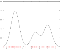
(a) Density function

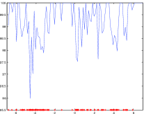
(b) $\beta=0.1$

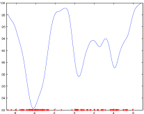
(c) $\beta=1$

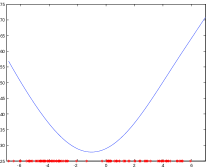
(d) $\beta=10$

Figure 4. (a) The density function is a mixture of three normal distributions and 100 i.i.d. samples (red dots on the horizontal axis) from it. (b)-(d) Graphs of $\sum_{i}d_{\beta}(x_{i},m)^{2}$ against $m$ for different values of $\beta$.

4.2. The general case: metric cone

The above construction is a special case of a general construction that applies to any geodesic metric space and hence to those in this paper. Let $\mathcal{X}$ be a geodesic metric space with a metric $d_{\mathcal{X}}$. A metric cone $\tilde{\mathcal{X}}_{\beta}$ with $\beta\in(0,\infty)$ is a cone $\mathcal{X}\times[0,1]/\mathcal{X}\times\{0\}$ with a metric

$$\tilde{d}_{\beta}((x,s),(y,t))$$

$$=\frac{1}{2}\sqrt{t^{2}+s^{2}-2ts\cos(\pi\min(d_{\mathcal{X}}(x,y)/\beta,1))}$$

for any $(x,s),(y,t)\in\tilde{\mathcal{X}}_{\beta}$.

The intuitive explanation is as follows. See Figure 5. Let $\mathcal{X}_{\beta}$ be the subset $\{(x,1)\mid(x,t)\in\tilde{\mathcal{X}}_{\beta}\}$ with the extrinsic geodesic metric on $\tilde{\mathcal{X}}_{\beta}$. Thus, $\mathcal{X}_{\beta}$ and $\mathcal{X}$ are the same as a set but endowing different metrics. Since $\tilde{d}_{\beta}((x,1),(y,1))=g_{\beta}(d_{\mathcal{X}}(x,y))$, $\mathcal{X}_{\beta}$ is a rescaling of the metric on $\mathcal{X}$ by $\beta$. For any $(x,s),(y,t)\in\tilde{\mathcal{X}}_{\beta}$, their projections $(x,1),(y,1)$ give two points $x,y\in\mathcal{X}$, respectively. For a geodesic $\gamma\subset\mathcal{X}$ between $x$ and $y$, consider a cone $\{(z,s)\mid z\in\gamma,s\in[0,1]\}$ spanned by $\gamma$. This cone can be isometrically embedded into an “extended unit circular sector”, i.e. a covering $\{(r,\theta)\mid r\in[0,1],\theta\in(-\infty,\infty)\}/\{(0,\theta)\mid\theta\in(-\infty,\infty)\}$ of the unit disk corresponding to $\theta\in[0,\pi d_{\mathcal{X}}(x,y)/\beta]$. Then $(x,s)$ and $(y,t)$ are also mapped into the extended unit circular sector; the distance $\tilde{d}_{\beta}((x,s),(y,t))$ for $\beta=1$ corresponds to the case (D2) of a disk if we set $(r,r^{\prime})=(s,t)$ and $(\theta,\theta^{\prime})=(\pi x,\pi y)$. This corresponds to the length of the blue line path in Figure 5 (b1) and (b2). For further details on metric cones, refer to Deza and Deza (2009).

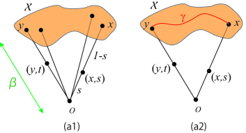
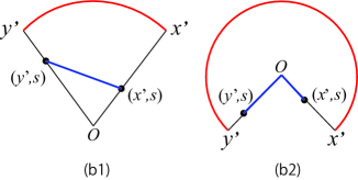
Figure 5. How to define a metric cone for a geodesic metric space $\mathcal{X}$.

The following result indicates that the metric cone space preserves the CAT(0) property of the original space and the smaller values of $\beta$ continue this process.

Theorem 4.1.

1. If $\mathcal{X}$ is a CAT(0) space, the metric cone $\tilde{\mathcal{X}}_{\beta}$ is also CAT(0) for every $\beta\in(0,\infty)$.

2. If $\tilde{\mathcal{X}}_{\beta_{2}}$ is CAT(0), $\tilde{\mathcal{X}}_{\beta_{1}}$ is also CAT(0) for $\beta_{1}<\beta_{2}$.

3. If $\mathcal{X}$ is CAT($k$) for $k\geq 0$, $\tilde{\mathcal{X}}_{\beta}$ becomes CAT(0) for $\beta\leq\pi/\sqrt{k}$.

The proof is given in appendix A.

It should be stressed that the theorems on $\beta$ cover metric cones based on an arbitrary geodesic metric space. If we start with the Euclidean graph as our geodesic space, it may not be CAT(0), but it can be shown that it is a CAT($k$) space for some $k$ and will eventually be CAT(0) for sufficiently small $\beta$.

5. CAT($k$) spaces, curvature, diameter and uniqueness of means

In this section we prove relation between the CAT($k$) property and the uniqueness of the intrinsic means. Let $\mathcal{X}$ be a geodesic metric space and fix it throughout this section. The diameter of a subset $A\subset\mathcal{X}$ is defined as the length of the longest geodesic in $A$. We define classes $\mathcal{C}_{\rm convex}$, $\mathcal{C}_{L_{\gamma}}$ and $\mathcal{C}_{\rm geodesic}$ as follows.

1. $\mathcal{C}_{\rm convex}$: the class of subsets $A\subset\mathcal{X}$ such that the geodesic distance function $f_{p}(x):=d(p,x)$ is strictly convex on $A$ for each $p\in A$. Here, “convex” means geodesic convex, i.e. a function $f$ on $\mathcal{X}$ is convex iff for every geodesic $\{\gamma(t)\mid t\in(t_{0},t_{1})\}$ on $\mathcal{X}$, $f(\gamma(t))$ is convex with respect to $t$.

2. $\mathcal{C}_{L_{\gamma}}$ for $\gamma\in[1,\infty]$: the class of the subsets $A\subset\mathcal{X}$ such that for any probability measure whose support is in $A$ and non-empty, the intrinsic $L_{\gamma}$-mean

   $$\mu=\mathop{\arg\min}_{m\in\mathcal{X}}E[d(X,m)^{\gamma}]$$

   exists uniquely. We refer to $\mathcal{C}_{L_{2}}$ as $\mathcal{C}_{\rm mean}$.

3. $\mathcal{C}_{\rm geodesic}$: the class of subsets $A\subset\mathcal{X}$ such that for every pair $p,q\in A$, the geodesic between $p$ and $q$ is unique.

Lemma 5.1.

$$\mathcal{C}_{\rm convex}\subset\mathcal{C}_{L_{\gamma}}\subset\mathcal{C}_{\rm geodesic}$$

for any $\gamma\in[1,\infty]$.

Proof.

If $A\in\mathcal{C}_{\rm convex}$, $f_{y}(x)=d(y,x)$ is a strictly convex function on $A$ for each $y\in A$; hence, $\int d(y,x)\mathrm{d}\mu_{Y}$ is strictly convex for any probability measure $\mu$ whose support is in $A$ and non-empty. Thus, $A\in\mathcal{C}_{L_{\gamma}}$. Next, assume that $B\notin\mathcal{C}_{\rm geodesic}$ and $x,y\in B$; then, there are at least two different geodesics, $\gamma_{1}$ and $\gamma_{2}$, between $x$ and $y$. Thus, there are two points $x^{\prime}$ and $y^{\prime}$ in $\gamma_{1}\cap\gamma_{2}$ such that there is no intersection of $\gamma_{1}$ and $\gamma_{2}$ between $x^{\prime}$ and $y^{\prime}$. Then, the mid points of $x^{\prime}$ and $y^{\prime}$ on each geodesic become intrinsic $L_{\gamma}$-means of the measure with two equal point masses on $x^{\prime}$ and $y^{\prime}$. This implies that $B\notin\mathcal{C}_{L_{\gamma}}$. ∎

Let $D_{\rm convex},D_{L_{\gamma}}$ and $D_{\rm geodesic}$ be the largest values (including $\infty$) such that every subset whose diameter is less than the value belongs to $\mathcal{C}_{\rm convex},\mathcal{C}_{L_{\gamma}}$ and $\mathcal{C}_{\rm geodesic}$, respectively. Then, evidently from Lemma 5.1, $D_{\rm convex}\leq D_{L_{\gamma}}\leq D_{\rm geodesic}$ for $1\leq\gamma\leq\infty$.

Note that if $\mathcal{X}$ is CAT(0), $D_{\rm convex}=D_{L_{\gamma}}=D_{\rm geodesic}=\infty$. In general, the following theorem holds.

Theorem 5.2.

• If $\mathcal{X}$ is CAT($k$), $D_{\rm convex}\geq\pi/(2\sqrt{\max(k,0)})$.

• If $\mathcal{X}$ is CAT($k$), $D_{\rm geodesic}\geq\pi/\sqrt{\max(k,0)}$.

• If $\mathcal{X}$ is a surface with a constant curvature $k>0$, $D_{L_{1}}\geq\pi/(2\sqrt{k})$.

Some parts of Theorem 5.2 are know results. See appendix B for details. The proof is also given in appendix B. By Theorem 5.2(1), $D_{L_{\gamma}}\geq D_{\rm convex}\geq\pi/(2\sqrt{k})$. Thus, a lower curvature $k$ gives a wider area where the intrinsic $L_{\gamma}$-mean is unique. According to Theorem 5.2(3), this lower bound for $D_{L_{1}}$ is the best universal upper bound for any $\mathcal{X}$ with CAT($k$) property.

For $\gamma>1$, $D_{L_{\gamma}}$ is bounded above by $(\theta_{0}(\gamma)+\pi/2)/\sqrt{k}$ where $\theta_{0}$ is an increasing function of $\gamma$ as shown in Figure 6. This bound is proved in appendix C. The upper bound shows that the parameter $\gamma$ plays a role in controlling the uniqueness of the mean, but it does not do so in Euclidean space, where the $L_{\gamma}$-mean functions are always convex.

Figure 6. Graph of $\theta_{0}(\gamma)$.

6. Choosing $\alpha$ and $\beta$

Combining the two deformations by $\alpha$ and $\beta$, we proposed a class of deformed metrics

$$d_{\alpha\beta}(x,y)=g_{\beta}(d_{\alpha}(x,y)).$$

If we use these metrics, the Fréchet function becomes

$$f_{\alpha\beta\gamma}(m)=\sum_{i=1}^{n}\{g_{\beta}(d_{\alpha}(x_{i},m))\}^{\gamma}$$

and the corresponding Fréchet mean and generalized variance are proposed:

$$\hat{\mu}=\arg\min_{m\in\mathcal{M}}f_{\alpha\beta\gamma}(m)~{}~{}\mbox{and}~{}~{}{\rm Var}_{\alpha\beta\gamma}=\displaystyle\min_{m\in\mathcal{M}}\frac{1}{n}f_{\alpha\beta\gamma}(m).$$

As explained in the previous sections, since $\alpha$ changes the curvature of the original data space and $\beta$ changes the curvature of a metric cone embedding the data space. Thus by tuning the values of $\alpha$ and $\beta$ we can control the uniqueness of the Fréchet function via the curvatures of these two geodesic metric spaces.

In this section, we suggest how to select the values of $\alpha$ and $\beta$ empirically from the data. For classification analysis with labels, the cross validation can be used to tune $\alpha$ and $\beta$. Thus we will focus on the case of cluster analysis, the Fréchet mean and the generalized variance.

6.1. Choosing $\alpha$

First, assume that we have Euclidean data (equivalent to $\beta=\infty)$ and recall the basic effect of decreasing $\alpha$ from $0$ to $-\infty$. At $\alpha=0$, we make no change to the metric. As $\alpha$ decreases, we lose edges from the geodesic graph. That is to say from time to time, an edge that is in a particular geodesic is discarded and every geodesic that passes through that edge then has to use an alternative route.

Let us assume that at $\alpha$ (and under mild extra conditions), only a single edge $e_{0}$ is removed and let $d_{0}^{1-\alpha}$ be its length. Let $d_{1}^{1-\alpha},\ldots,d_{k}^{1-\alpha}$ be the lengths of the edges on the new geodesic that will replace the removed edge. In addition, let there be $n_{0}$ distinct geodesics that use $e_{0}$. It is straightforward to see that all geodesics that use $e_{0}$ will use the new arc for an interval $[\alpha,\alpha+\epsilon)$, for sufficiently small $\epsilon>0$. The total change in geodesic length is

$$\Delta(\alpha)=n_{0}(d_{0}^{1-\alpha}-\sum_{i=1}^{k}d_{i}^{1-\alpha}),$$

and it is continuous at the current $\alpha$ but the first derivative changes: $\Delta^{\prime}(\alpha)$ is typically not zero. To see this, take the case where all the $d_{i},i=1,\ldots,k,$ are equal. Then, the change in the first derivative is

$$-\frac{n_{0}d_{0}^{1-\alpha}}{1-\alpha}\log k.$$

In graph theory, the number of geodesics using a particular edge, $n_{0}$ in our case, is sometimes called the edge betweenness. We might therefore refer to the term $n_{0}d_{0}^{1-\alpha}$ as the weighted betweenness. This quantity measures changes in the configuration: if $n_{0}$ and $d_{0}^{1-\alpha}$ are large then a long edge with large betweenness is removed, and it is replaced by $k$ shorter edges from the current geodesic graph.

If $n_{e}$ is the betweenness of an edge $e$, the total betweenness of a graph $G(V,E)$ is the sum of all the individual edge betweennesses, $\displaystyle\sum_{e\in E}n_{e},$ and the weighted version is $\displaystyle\sum_{e\in E}n_{e}d_{e}^{1-\alpha},$ which except for a scalar factor is the $L_{1}$ variance given by $\gamma=1$, in this paper.

We shall in fact favour the use of $s_{1}$ ($\gamma=2)$, and with the above discussion in mind, we will see in Examples 1 and 2 that plots of the second derivative of $\log s_{1}$ do indeed have pronounced peaks and there is some matching of the $\alpha$-values at the peaks with the analogous differential of the aggregate betweenness.

6.2. Choosing $\beta$

Section 4.1 and Figure 4 are important for understanding the $\beta$ metric. We can summarise the material in a way that will indicate how to estimate $\beta$. The first point is that $\beta$ provides a metric cone. In one dimension, we wrap the real line around a circle and attach the origin. Then, the metric cone is based on the Euclidean metric inside the cone. The enlarged space (referred to as the embedding space) is CAT(0) with respect to this metric.

We claim that this construction is fundamental because even in larger spaces, the geodesics are one-dimensional. Every geodesic, in some sense, has its private cone but they all have a common vertex. Moreover, by Theorem 4.1, if the base space is CAT(0), the embedding space is CAT(0), and in both cases, we have a unique intrinsic mean and our statistics are well defined. However, if we compute the intrinsic mean restricted to the base space, e.g. Euclidean space, then the uniqueness no longer holds. As stated above, the space may not be CAT(0) for small $\beta$ but may become more so for large $\beta$. We can use this to our advantage: for sufficiently large $\beta$, we expect a single minimum

$$f_{\beta}(m)=\sum_{i=1}^{n}g_{\beta}(d(x_{i},m))^{2},$$

but multiple minima for smaller $\beta$, as shown in Figure 4. If we recall that the value of the function $f_{\beta}$ for a given $\beta$ is helpful in clustering, we can suggest a number of plots to show the local minima.

However, we can say more. First, note that in one dimension,

$$W_{\beta}(|x|)=\frac{1}{\beta}(1-g_{\beta}(|x|)^{2})=\frac{1}{2}\cos^{2}\left(\frac{\pi|x|}{2\beta}\right)$$

over $[-\beta,\beta]$ is a smooth kernel with bandwidth $\beta$. Thus, with $d(x_{i},m)=|x_{i}-m|$, we see that

$$\frac{1}{\beta}\left(1-\frac{f_{\beta}(x)}{n}\right)=\frac{1}{n}\sum_{i}W_{\beta}(|x_{i}-x|)$$

is a smooth density. This interpretation helps to intuitively choose $\beta$: select a “typical value” of $\|x_{i}-x\|$, e.g. the average of $\|x_{i}-x_{j}\|$, by analogy with bandwidth selection for kernel functions.

Another option is to use cycle lengths in the geodesic graph. As can be seen from Theorem 3.3 and the proof of Theorem 4.1, if we set $\beta=|\Gamma|/2\pi$ for a cycle $\gamma$ and its length $|\Gamma|$, then the metric cone generated by the cycle becomes CAT(0). The use of $\beta$ is shown in Examples 1 and 3.

7. Examples

In this section, we apply the $d_{\alpha,\beta,\gamma}$ metric to real data. Because the $L^{\gamma}$ loss function is more familiar than deformation of metrics by $\alpha$ and $\beta$, we will set $\gamma=2$ and focus on $\alpha$ and $\beta$ throughout the section.

For the $d_{\alpha}$ metric (for $\beta=\infty$, $\gamma=2$), we briefly describe the computation. For each fixed $\alpha$ and each pair of points initially every $d_{\alpha}(x_{i},x_{j})$ is computed, giving a complete graph. On this graph the $x_{i}$ to $x_{j}$ geodesic is computed for all $i\neq j$. The geodesic graph, for this $\alpha$, is then computed as the union of all such geodesics. The present version of the software computes the geodesic graph for a grid of around 100 points, depending on the range of $\alpha$. As mentioned, we are interested, here, only in the range $(-\infty,1]$ and typically consider the range $(-r,1]$, where $r$ is a small positive integer. For each $\alpha$, we compute $s_{0}^{2}$ and $s_{1}^{2}$.

7.1. Example 1: $k$-nearest neighbour classification with $d_{\alpha,\beta}$

We apply the $d_{\alpha,\beta}$ metric to the $k$-nearest neighbour ($k$-NN) method, one of the simplest and most popular classification methods. We will see that if we can choose adequate values for $\alpha$ and $\beta$, the classification error can be reduced.

We use five data sets from he UCI Machine Learning Repository (Bache and Lichman (2013)): (i) Fisher’s iris data set (number of instances $n=150$, number of attributes $d=4$, number of clusters $m=3$), (ii) wine data set ($n=178$, $d=13$, $m=3$), (iii) ionosphere data set ($n=351$, $d=32$, $m=2$), with only real attributes, (iv) breast cancer Wisconsin (diagnostic) data set ($n=569$, $d=30$, $m=2$), and (v) yeast data set ($n=1484$, $d=8$, $m=10$). The average $l^{2}$ norm of each data set is normalized to be one.

The Euclidean complete graphs are used as the initial metric graphs ($\alpha=0$), and classification is performed using the weighted $k$-NN method ($k$=10) with a common weighting $1/d^{2}$ where $d$ is the distance to the neighbour data point but using $d_{\alpha,\beta}$ for various values of $\alpha\in\{-5,-4.8,\dots,0.8,1\}$ and $\beta\in\{2^{-6},2^{-2},\dots,2^{5},\infty\}$. A half of the samples is selected at random as a training set and the rest half is used as a testing set to evaluate the classification result. We repeat it 1000 times and estimate the error rate.

Table 2. Classification by $k$-NN method

	$k$-NN with $d_{\alpha,\beta}$			with Euclidean
data set	$\hat{\alpha}$	$\hat{\beta}$	$\hat{r}$	$r$
(i) iris	-4.4	0.0156	0.0334$\pm$0.0011	0.0366$\pm$0.0011
(ii) wine	0	$\infty$	0.2814$\pm$0.0025	0.2814$\pm$0.0025
(iii) ionosphere	-0.4	$\infty$	0.1671$\pm$0.0018	0.1677$\pm$0.0018
(iv) cancer	0.4	2	0.0708$\pm$0.0008	0.0729$\pm$0.0007
(v) yeast	0.4	8	0.4184$\pm$0.0009	0.4227$\pm$0.0008

In Table 2, $\hat{\alpha}$ and $\hat{\beta}$ are the values attaining minimum mean classification error and $\hat{r}$ is the error rate with 95% confidence interval ($\pm 1.96(\mbox{std.})/\sqrt{1000}$) In addition, $r$ is the classification error for the ordinary Euclidean $k$-NN. The boldfaces represent significantly smaller error rates by $d_{\hat{\alpha},\hat{\beta}}$ than Euclidean $k$-NN.

Figure 7 shows the geodesic graphs of the first three data sets with the optimum values of $\alpha$ and $\beta$. To simplify the figures, 100 samples from each data set are randomly selected and the optimum values of $\alpha$ and $\beta$ are recomputed. The shape of the sample points represents their class (we use only three types of point shapes by using the same point shape for the third and higher labeled classes for clarity of the figures). The value of $f(x)=\sum_{i}g_{\beta}(d_{\alpha}(x_{i},x))^{2}$ at each sample point is represented by the different colours (red:small, blue:large). We can see that the shapes of the “optimal” geodesic graphs are variable because the optimal value of $\alpha$ depends on the original data spaces and the distributions.

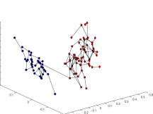
(a) iris ($\hat{\alpha}=-4.2,~{}\hat{\beta}=2^{-4}$)

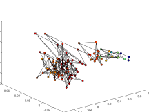
(b) wine ($\hat{\alpha}=-0.4,\hat{\beta}=\infty$)

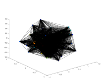
(c) ionosphere ($\hat{\alpha}=0.8,\hat{\beta}=\infty$)

Figure 7. The geodesic graph of each data set with an optimum value of $\alpha$ and $\beta$.

The computation cost is linear in the number $d$ of attributes and therefore, the number $n$ of samples is our main concern. The heaviest part of the algorithm is to compute the shortest path length between each pair of samples. We used Floyd’s algorithm (Floyd (1962)) which requires $O(n^{3})$ computations.

There is a need for a more efficient program for more than 10,000 samples. One option is to begin from the subgraph of the complete graph: for example, the union of the complete subgraph whose vertices are a subset of the samples and the edges connecting the remaining samples to the complete subgraph. Moreover, if we can decrease the number of edges in the geodesic graphs, Johnson’s algorithm for computing the shortest path lengths can be used instead of Floyd’s algorithm, because it requires only $O(|E|n+n^{2}\log n)$, where $|E|$ is the number of edges.

7.2. Example 2: Clustering of the world population

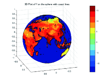
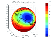
$\beta=1$

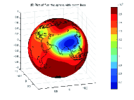
$\beta=0.3$

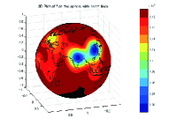
$\beta=0.1$

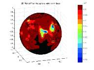
$\beta=0.01$

Figure 8. (left) the population density, (right) the Fréchet function for $\beta=1,0.3,0.1,0.01$

We will show how $\beta$ plays a role in clustering analysis by using a toy example of world population. We used the data “Population Count Grid, v3 (2000)” by NASA (downloadable from CIESEN et al (2005)). The resolution of the angle is 1 degree both for the latitude and the longitude. Figure 8 (left) shows the world population density computed from the data (high:red, low:blue). The colours in Figure 8 (right) represent the value of the Fréchet function,

$$f_{\beta}(m)=\sum_{i}g_{\beta}(\|x_{i}-m\|)^{2},$$

for $x_{i},m\in S^{2}$. Here the higher value of $f$ is red (lower population) and the lower value is blue (higher population).

We can see the Fréchet function has more local minima as $\beta$ becomes smaller. Thus if an adequate value of $\beta$ is selected, we can obtain the centres of a prescribed number of population clusters. As we have seen above, a smaller value of $\beta$ corresponds to a smaller curvature of the embedding metric cone in the sense of the CAT($k$) property. Thus this example shows how the curvature of the embedding metric cone affects the Fréchet function and the clustering analysis by the function.

7.3. Example 3: comparison of empirical graphs via connectedness and graph Ricci curvature

In this section, we compare the structure of empirical graphs computed by three different methods, the $\epsilon$-neighbourhood graph, the $k$-nearest neighbours graph and the $\alpha$-graph (geodesic subgraph) proposed in this paper. The $\epsilon$-neighbourhood graph is an undirected (empirical) graph such that two vertexes are connected if the distance of the two vertexes is smaller than a positive $\epsilon$. The $k$-nearest neighbours ($k$-NN) graph is an undirected (empirical) graph constructed by joining each vertex to its $k$ nearest neighbour vertexes. While the $\epsilon$-neighbourhood graph is a natural option for empirical graphs if the data points are almost uniformly distributed, the $k$-NN graph has several merits in application (e.g. the graph has usually fewer connected components) and is used more often especially for high dimensional data. It is worth to remark that the $k$-NN algorithm is the most popular method to construct empirical graphs in the area of manifold learning. See Section 1.2 and the references there for more details of the manifold learning.

We use three artificial data and one real data: (1) uniform sample on $[0,1]^{2}$, (2) uniform sample on $S^{2}\subset\mathbb{R}^{3}$, (3) uniform sample on a subset of $H^{2}\subset\mathbb{R}^{3}$ defined by the variety $x^{2}+y^{2}-z^{2}=1,(-1\leq z\leq 1)$ and (4) protein data 1BUW. Sample size for artificial data (1)-(3) is 500. (4) is a data of 3-d position of 4326 atoms in a hemoglobin protein (PDB-ID:1BUW) and downloaded from Protein Data Base(PDB) (see Berman et al (2000)).

Table 3 represents how the numbers of edges $e:=|E_{\nu}|$ and the number of connected components $c$ of the empirical graph $G_{\nu}:=(V,E_{\nu})$ for the three graph construction methods change with parameter value $\nu$. Here, $\nu=k$ for the $k$-NN, $\epsilon$ for the $\epsilon$-neighbourhood method and $\alpha$ for the $\alpha$-graph. We first compute the $k$-NN graph for $k=1,2,4$ and $8$ and next select the values for $\epsilon$ and $\alpha$ such that the corresponding graphs have a similar number of edges. For the $\epsilon$-neighbourhood and the $k$-NN graphs, the number of connected components changes with $\epsilon$ and $k$, respectively. As expected, the $\epsilon$-neighbourhood graph is less connected than the $k$-NN graph for non-Euclidean space. On the contrary, the $\alpha$-graph is connected for any value of $\alpha$. This is more evidently depicted by Figure 9 for the protein data. Moreover, we can see the number of edges in the $\alpha$-graphs changes monotonically and more smoothly than other two methods when we changes the parameter value $\nu$. This means the $\alpha$ for the $\alpha$-graph is preferable for controlling the number of edges in the empirical graph.

Table 3. Number of edges $e$ and connected components $c$ of empirical graphs for three graph construction methods with parameter $\nu$.

		$k$-NN ($\nu=k$)				$\epsilon$-neighbourhood ($\nu=\epsilon$)				$\alpha$-graph ($\nu=\alpha$)
Uniform	$\nu$	1	2	4	8	0.03	0.04	0.06	0.08	-10	-2.7	-0.5	-0.1
on $[0,1]^{2}$	$e$	348	652	1202	2300	333	585	1339	2366	523	649	1228	26523
$n=500$	$c$	152	29	1	1	247	124	6	1	1	1	1	1
Uniform	$\nu$	1	2	4	8	0.07	0.10	0.14	0.20	-10	-3.0	-0.6	-0.2
on $S^{2}$	$e$	347	648	1229	2389	340	697	1292	2470	521	643	1180	2098
$n=500$	$c$	153	27	1	1	318	215	118	17	1	1	1	1
Uniform	$\nu$	1	2	4	8	0.14	0.20	0.27	0.37	-10	-2.6	-0.5	-0.2
on $H^{2}$	$e$	350	647	1205	2370	341	666	1243	2353	519	645	1247	2322
$n=500$	$c$	150	24	1	1	244	112	34	11	1	1	1	1
Protein	$\nu$	1	2	4	8	1.6	2.3	2.7	3.7	-10	-2.3	-0.9	-0.5
1BUW	$e$	3194	5289	10556	20830	4420	5321	10563	20800	4446	5295	10198	21393
$n=4326$	$c$	1132	218	1	1	22	6	2	1	1	1	1	1

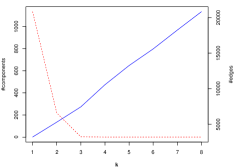
(a) $k$-NN

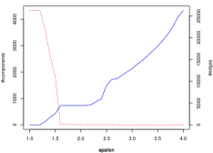
(b) $\epsilon$ neighbourhood

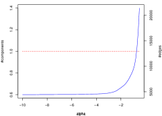
(c) $\alpha$-graph

Figure 9. The number of connected components (red dashed line, left axis) and edges (blue solid line, right axis) for various values of $\epsilon$, $k$ and $\alpha$, respectively, for the protein data.

Next we compare the three types of empirical graphs via the graph Ricci curvature proposed in Lin et al (2011). The graph Ricci curvature for each pair of vertexes is defined by using the graph Wasserstein metric on the graph and has some analogy to the Ricci curvature on Riemannian manifolds. We compute the Ricci curvature for every edge in the empirical graphs for data (3) and (4). In Fig. 10 for data (3) and Fig. 11 for data (4), each edge is coloured (blue:small, red:large) by its Ricci curvature for the three types of empirical graphs. Here the parameters are selected from Table 3 as $k=4$, $\epsilon=0.27$, $\alpha=-0.5$ for Fig. 10 and $k=4$, $\epsilon=2.7$, $\alpha=-0.9$ for Fig. 11. The histogram of Ricci curvatures for all edges of each empirical graph is displayed under the graph. Each histogram seems to converge to normal distribution (this is surprising for us) and the histogram for $\alpha$-graph converges faster than other two. We expect the reason for this property is partly because the $\alpha$ controls the CAT($k$) property, another kind of curvature but related to Ricci curvature, of $\alpha$-graphs. We remark that Ricci curvatures in the $\alpha$-graphs for $\alpha<0$ tend to have some negative bias for our examples. This is reasonable when we remember a negative value of $\alpha$ makes the data space more CAT($k$).

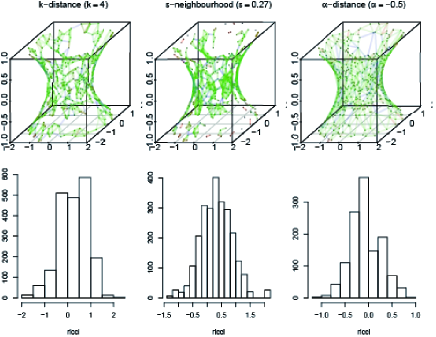
Figure 10. The Ricci curvature of each edge (red:large, blue:small) for Uniform sample on $H^{2}$

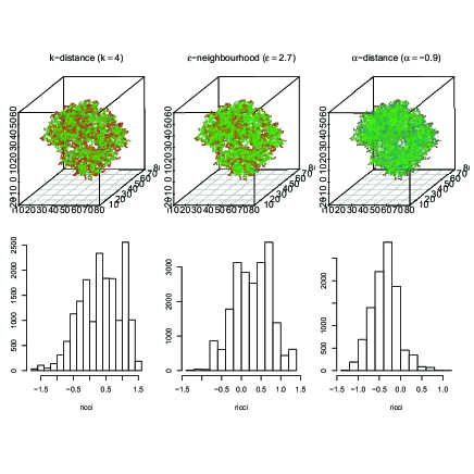
Figure 11. The Ricci curvature of each edge (red:large, blue:small) for the protein data (1BUW)

7.4. Example 4: Rainfall data

We carry out some analysis of rainfall (precipitation) data obtained from the UK Met Office Hadley Centre (downloadable from Alexander and Jones (2000)). Considering a single year’s data we take the “dimensions” as the nine regions of the UK: South East England, South West England and Wales, Central England, North West England and Wales, North East England, South Scotland, North Scotland, East Scotland and Northern Ireland, and the “points” as the 365 (or 366) days of the year. We take the years 1931 to 2014. Initially, we select values of $\alpha=0,-0.1,-0.22,-1$ by using some peaks of $-(\log s_{1})^{\prime\prime}$ in Figure 12. For each year, we compute $s_{0}^{2/(1-\alpha)}$ for values $\alpha=0,-0.1,-0.22,-1$. The data is presented as four time series with different values of $\alpha$ for yearly values from 1931 to 2014 in Figure 13. The figure is consistent with an emerging consensus of increased extremes and volatility in precipitation in the UK in recent years (see Met Office, 2014,“Recent Storms Briefin”).

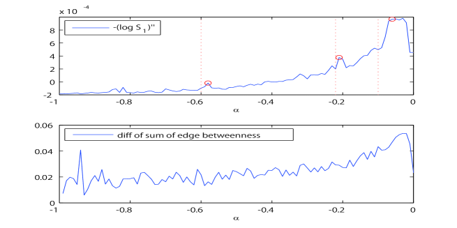
Figure 12. Selecting $\alpha$ for weather data of 2014. Upper graphs: selected peaks of $-\log{s_{1}}^{\prime\prime}$ (marked as circles) and values of $\alpha$ (dashed lines). Lower graphs: numerical differentiation of the sum of betweenness of each edge with respect to $\alpha$.

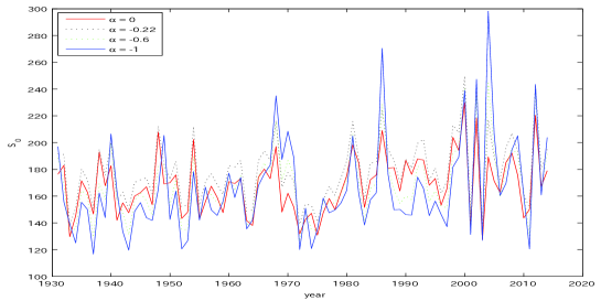
Figure 13. Rainfall data in UK (1931-2014): yearly time series of $s_{0}^{2/(\alpha-1)}$ plotted for $\alpha=0$ (red solid line), $-0.1$ (green dashed line), $-0.6$ (black dashed line) and $-1$ (blue solid line).

We now discuss the choice of $\alpha$. Following the discussion in Figure 12, we plot $-\frac{\partial^{2}}{\partial\alpha^{2}}\log s_{1}$ in the range $\alpha\in[-1,0]$. Figure 12 shows plots for the year 2014. We select the values of $\alpha$ to be slightly smaller than the peaks. The local peak at approximately $\alpha=-0.22$ indicates a rapid change in the topology of the graph at this point: we lose a considerable number of longer edges and reveal the structure in the data as a consequence. The betweenness plot is not so revealing, except near $\alpha=-1$.

8. Conclusion

The $\alpha$ metric is a deformation of the starting geodesic, and as $\alpha$ becomes more negative, the geodesic graph, namely the union of all the geodesics, becomes sparser, and in our graph representation, it becomes a tree. The space is CAT($k$) with smaller $k$ and finally becomes a tree, at which point the space becomes CAT(0). It is quite difficult to see the tree computation because of the numerous short edges, but for moderate values of $\alpha$ such as $-1$, the structure is tree-like. Abrupt changes in various statistics as $\alpha$ changes reveal topological changes in the structure of the geodesic graph, a fact that can be used to tune $\alpha$.

The $\beta$ metric is “non-geodesic” because although the function $g_{\beta}$ operates on a geodesic, that does not mean that the space is a geodesic space in the formal sense. However the cone construction yields a geodesic metric space, which is CAT($k$) with a lower value of $k$ than the original space, and indeed may be CAT(0). If the $\beta$ metric is projected back to the original space, that space can have a non-convex Fréchet function with larger $k$. This is useful for finding clusters because of multiple minima of the Fréchet function, which is itself similar to a kernel. The means obtained by the $\beta$-metric may represent the first study of an extrinsic mean via embedding in non-Euclidean spaces and the first application of metric cones to statistics and data analysis.

We believe that the curvature of the data space underlying this work demands further investigation whereby connections should be established with recent developments related to empirical geodesic graphs, for example in manifold learning. One important direction should be the effect of the curvature of the space on the trade-off between the uniqueness of the Fréchet means and the robustness of estimation. To this end, $\alpha,\beta$ and $\gamma$ can be seen as parameters that can be tuned to change the curvature and hence study the trade-off.

Appendix A Proof of Theorem 4.1

(1) Denote the mapped points of $a,b,c$ and $x$ by the projection $\tilde{\mathcal{X}}_{\beta}\rightarrow\mathcal{X}_{\beta}$ as $A,B,C$ and $X$, respectively, as shown in Figure 14 (left). Denote the origin of the metric cone as $O$. If the sum of the lengths of the geodesics $\widetilde{AB}$, $\widetilde{AC}$ and $\widetilde{BC}$ in $\mathcal{X}_{\beta}$ exceeds $2\pi\beta$, it is easy to see that the cone spanned by $\overline{ab}\cup\overline{ac}\cup\overline{bc}$ becomes CAT(0) and $\Delta abc$ satisfies the CAT(0) property. Therefore, assume that $|\widetilde{AB}|+|\widetilde{AC}|+|\widetilde{BC}|\leq 2\pi\beta$.

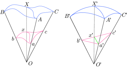
Figure 14. The cone spanned by geodesics $\overline{ab}$, $\overline{ac}$, $\overline{bc}$ and $\overline{ax}$ (left) and the cone spanned by a comparison triangle $\Delta a^{\prime}b^{\prime}c^{\prime}$ (right).

Next, let $\Delta a^{\prime}b^{\prime}c^{\prime}$ be a comparison triangle of $\Delta abc$ and let $x^{\prime}$ be a point on a geodesic $\overline{b^{\prime}c^{\prime}}$ such that $|\overline{bx}|=|\overline{b^{\prime}x^{\prime}}|$. Thus, $|\overline{a^{\prime}x^{\prime}}|<|\overline{ax}|$. Arrange the points $a^{\prime}$, $b^{\prime}$ and $c^{\prime}$ in a three-dimensional Euclidean space with origin $O^{\prime}$ such that the lengths of $\overline{O^{\prime}a^{\prime}}$, $\overline{O^{\prime}b^{\prime}}$ and $\overline{O^{\prime}c^{\prime}}$ are equal to the lengths of $\overline{Oa}$, $\overline{Ob}$ and $\overline{Oc}$, respectively. Denote the radial projection of $a^{\prime}$, $b^{\prime}$, $c^{\prime}$ and $x^{\prime}$ to a unit sphere as $A^{\prime}$, $B^{\prime}$, $C^{\prime}$ and $X^{\prime}$, respectively, as shown in Figure 14 (right). By the definition of a metric cone, $|\overline{Ox}|=|\overline{O^{\prime}x^{\prime}}|$ and the geodesics $\widetilde{A^{\prime}B^{\prime}}$, $\widetilde{A^{\prime}C^{\prime}}$, $\widetilde{B^{\prime}C^{\prime}}$ and $\widetilde{A^{\prime}X^{\prime}}$ in the unit sphere are arcs satisfying $|\widetilde{A^{\prime}B^{\prime}}|=|\widetilde{AB}|$, $|\widetilde{A^{\prime}C^{\prime}}|=|\widetilde{AC}|$, $|\widetilde{B^{\prime}C^{\prime}}|=|\widetilde{BC}|$ and $|\widetilde{B^{\prime}X^{\prime}}|=|\widetilde{BX}|$.

From the argument above, $|\widetilde{A^{\prime}B^{\prime}}|+|\widetilde{A^{\prime}C^{\prime}}|+|\widetilde{B^{\prime}C^{\prime}}|=|\widetilde{AB}|+|\widetilde{AC}|+|\widetilde{BC}|\leq 2\pi$. Since the unit sphere has a positive constant curvature and $\mathcal{X}_{\beta}$ is CAT(0), $|\widetilde{A^{\prime}X^{\prime}}|>|\widetilde{AX}|$. However, since $|\overline{Oa}|=|\overline{O^{\prime}a^{\prime}}|$ and $|\overline{Ox}|=|\overline{O^{\prime}x^{\prime}}|$, $|\widetilde{A^{\prime}X^{\prime}}|>|\widetilde{AX}|$ implies that $|\widetilde{a^{\prime}x^{\prime}}|>|\widetilde{ax}|$ by the property of a metric cone. Thus, $\Delta abc$ has CAT(0) property and (1) of the theorem is proved.

(2) Assume that $0<\beta_{1}<\beta_{2}<\infty$ and a metric cone $\tilde{\mathcal{X}}_{\beta_{1}}$ is not CAT(0) for proving the latter half of the theorem by contradiction. Then, there is a geodesic triangle $\Delta a_{1}b_{1}c_{1}$ in $\tilde{\mathcal{X}}_{\beta_{1}}$ and a point $x_{1}$ on the geodesic $\overline{b_{1}c_{1}}$ such that the geodesic $\overline{a_{1}x_{1}}$ is longer than the corresponding geodesic of a comparison triangle. By defining $A_{1},B_{1},C_{1},X_{1},a^{\prime}_{1},b^{\prime}_{1},c^{\prime}_{1},x^{\prime}_{1},A^{\prime}_{1},B^{\prime}_{1},C^{\prime}_{1}$ and $X^{\prime}_{1}$ as above, we can say that $|\widetilde{A_{1}X_{1}}|>|\widetilde{A^{\prime}_{1}X^{\prime}_{1}}|$.

Next, each of $A_{1},B_{1},C_{1}$ and $X_{1}$ corresponds to a point in $\mathcal{X}_{\beta_{1}}$ and we can consider the corresponding points $A_{2},B_{2},C_{2}$ and $X_{2}$ in the other metric cone $\tilde{\mathcal{X}}_{\beta_{2}}$. When restricted to $\mathcal{X}_{\beta_{1}}$, a geodesic $\widetilde{A_{1}X_{1}}$ is just a rescaling of $\widetilde{A_{2}X_{2}}$ and $|\widetilde{A_{1}X_{1}}|=\frac{\beta_{1}}{\beta_{2}}|\widetilde{A_{2}X_{2}}|$.

Now, $\Delta A_{2}^{\prime}B_{2}^{\prime}C_{2}^{\prime}$ is a geodesic triangle on the unit sphere, but after rescaling by $\frac{\beta_{2}}{\beta_{1}}$, we can get a geodesic triangle $\Delta A_{2}^{\prime\prime}B_{2}^{\prime\prime}C_{2}^{\prime\prime}$ on a sphere of radius $\frac{\beta_{2}}{\beta_{1}}$ whose edges have the same length as $\Delta A_{1}^{\prime}B_{1}^{\prime}C_{1}^{\prime}$. By a known result on spherical triangles with the same edge lengths on different spheres, a larger radius implies a “thinner” triangle and $|\widetilde{A_{1}X_{1}}|<|\widetilde{A_{2}^{\prime\prime}X_{2}^{\prime\prime}}|$ where $X_{2}^{\prime\prime}$ is a point on the geodesic $\widetilde{B_{2}^{\prime\prime}C_{2}^{\prime\prime}}$ such that $|\widetilde{B_{1}X_{1}}|=|\widetilde{B_{2}^{\prime\prime}X_{2}^{\prime\prime}}|$.

Combining all the arguments gives

$$\textstyle|\widetilde{A_{2}X_{2}}|=\frac{\beta_{2}}{\beta_{1}}|\widetilde{A_{1}X_{1}}|>\frac{\beta_{2}}{\beta_{1}}|\widetilde{A^{\prime}_{1}X^{\prime}_{1}}|>\frac{\beta_{2}}{\beta_{1}}|\widetilde{A_{2}^{\prime\prime}X_{2}^{\prime\prime}}|=|\widetilde{A^{\prime}_{2}X^{\prime}_{2}}|.$$

Select a non-degenerate geodesic triangle in $\tilde{\mathcal{X}}_{\beta_{2}}$ by selecting arbitrary points $a_{2},b_{2}$ and $c_{2}$ on the geodesics $\overline{OA_{2}}$, $\overline{OB_{2}}$ and $\overline{OC_{2}}$ in $\tilde{\mathcal{X}}_{\beta_{2}}$, respectively, and let $x_{2}$ be the intersection point of $\overline{OX_{2}}$ and $\overline{b_{2}c_{2}}$. Then, by $|\widetilde{A_{2}X_{2}}|>|\widetilde{A^{\prime}_{2}X^{\prime}_{2}}|$, we can say that $|\overline{a_{2}x_{2}}|>|\overline{a^{\prime}_{2}x^{\prime}_{2}}|$. This implies that $\tilde{\mathcal{X}}_{\beta_{2}}$ is not CAT(0) and (2) of the theorem is proved.

(3) For $k=0$, the statement holds by (1). For $k>0$ and $\beta\leq\pi$, it is sufficient to prove for $\beta=\pi/\sqrt{k}$ by (2). Let $\Delta abc$ be a geodesic triangle in $\tilde{\mathcal{X}}_{\beta}$ and let $\Delta ABC$ be a geodesic triangle in $\mathcal{X}_{\beta}$. Let $A,B,C$ be the projection of $a,b,c$, respectively. If the perimeter of $\Delta ABC$ is longer than or equal to $2\pi$, the cone spanned by the perimeter becomes CAT(0) by the same argument as that for (1). Therefore, $\Delta abc$ is CAT(0) and satisfies the CAT(0) property.

If the perimeter of $\Delta ABC$ is smaller than $2\pi$, since $\mathcal{X}$ is CAT($k$) and $\mathcal{X}_{\beta}$ is CAT(1), for any $X\in\widetilde{BC}$, $\widetilde{BX}$ is shorter than the corresponding great arc $\widetilde{B^{\prime}X^{\prime}}$ of a comparison triangle $\Delta A^{\prime}B^{\prime}C^{\prime}$, which is a spherical triangle on the unit sphere. Since a comparison triangle $\Delta a^{\prime}b^{\prime}c^{\prime}$ of $\Delta abc$ can be embedded on the cone spanned by $\Delta A^{\prime}B^{\prime}C^{\prime}$, $\widetilde{bx}$ is shorter than the corresponding line segment $\widetilde{b^{\prime}x^{\prime}}$. This means the $\Delta abc$ satisfies the CAT(0) property. ∎

Appendix B Proof of Theorem 5.2

(1) Although this is a known result, for example Kendall (1990) Espínola and Fernández-León (2009), we show a short proof. Since a comparison triangle for the CAT($k$) property is on a sphere of radius $1/\sqrt{k}$, first consider the unit sphere $S^{2}$ and the geodesic distance $d$ on it. Take three points $a,b,c\in S^{2}$ and think of the convexity of $d(x,a)$ for $x\in\widetilde{bc}$. Without losing generality, assume that $a$ is on the plane $y=0$ and $\widetilde{bc}$ is on the plane $z=0$ and let $b=(\cos\theta_{0},\sin\theta_{0},0)$, $x=(\cos\theta,\sin\theta,0)$ and $a=(\cos\psi,0,\sin\psi)$ for $\theta_{0},\theta\in(-\pi,\pi]$,$\psi\in[-\pi/2,\pi/2]$.

Thus, $d(a,x)=\arccos(a^{\top}x)=\arccos(\cos\theta\cos\psi)$ and $d(b,x)=|\theta-\theta_{0}|$. Note that for $\psi=0$, $d(a,x)=|\theta|$ for $\psi=0$ is a convex of $d(b,x)$. For a $\psi\neq 0$, $d(a,x)\leq\pi/2$ for $x\in\widetilde{bc}$, $d(a,x)$ is a convex of $d(b,x)$ iff $a^{\top}x=\cos\theta\cos\psi\geq 0$ since $\frac{\partial^{2}}{\partial\theta^{2}}d(a,x)=\cos(\theta)\cos(\psi)\sin^{2}(\psi)(1-\cos^{2}\theta\cos^{2}\psi)^{-2/3}$. This means that if $d(a,x)\leq\pi/2$ for $x\in\widetilde{bc}$, $d(a,x)$ is a convex of $d(b,x)$.

If $\mathcal{X}$ is CAT($k$) and has a diameter of at most $\pi/(2\sqrt{k})$, there is a comparison triangle $\Delta a^{\prime}b^{\prime}c^{\prime}$ on a sphere of radius $1/\sqrt{k}$ such that its perimeter is at most $3\pi/(2\sqrt{k})$ and $d(a^{\prime},x^{\prime})$ is a convex of $d(b^{\prime},x^{\prime})$ for each $x^{\prime}\in\widetilde{b^{\prime}c^{\prime}}$ because of the argument above after scaling by $1/\sqrt{k}$.

(2) is well known. See Espínola and Fernández-León (2009).

(3) We show an example of the probability measure with a three-point support on $S^{2}$ such that the diameter is larger than $\pi/2$ but can be arbitrarily close to $\pi/2$ and the uniqueness of the intrinsic $L_{1}$-mean fails.

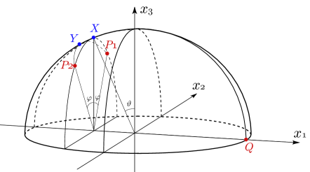
Figure 15. $P_{1}$,$P_{2}$,$Q$, $X$ and $Y$ on the unit hemisphere.

Take $Q=(1,0,0)$, $P_{1}=(-\sin\theta,\cos\theta\sin\psi,\cos\theta\cos\psi)$, $P_{2}=(-\sin\theta,\cos\theta\sin\psi,\cos\theta\cos\psi)$ and $X=(-\sin\theta,0,\cos\theta)$ with $\theta,\psi\in(0,\pi/2)$, as in Figure 15. Let $Y=(-\sin\theta^{\prime},0,\cos\theta^{\prime})$ be the mid point of $\widetilde{P_{1}P_{2}}$ for $\theta^{\prime}>\theta$. Put the point masses $m_{1}$ at $Q$ and $M$ at $P_{1}$ and $P_{2}$, and assume that there is a unique intrinsic median $\mu$.

By the symmetry, $\mu$ must be on the arc $\widetilde{QY}$, and if we change the ratio $M/m$, $\mu$ moves continuously on $\widetilde{QY}$. Thus, we can set $\mu=X$ by tuning $M/m$ adequately. However, $L_{1}$-dispersion from $X$ becomes $S_{X}=md(\theta,X)+Md(P_{1},X)+Md(P_{2},X)=m(\pi/2+\theta)+2M\psi$, and $L_{1}$-dispersion from $P_{1}$ becomes $S_{P_{1}}=md(\theta,P_{1})+Md(P_{2},P_{1})=m(\pi/2+\theta)+2M\psi$. This contradicts the assumption of $X$ being the unique $L_{1}$-intrinsic mean. Since we can set $\theta$ and $\psi$ as arbitrarily small positive numbers, $D_{L_{1}}\leq\pi/(2\sqrt{k})$. However, by (1), $D_{L_{1}}\geq D_{\rm convex}\geq\pi/(2\sqrt{k})$; thus, $D_{L_{1}}=\pi/(2\sqrt{k})$.∎

Appendix C An upper bound of $D_{L_{\gamma}}$

Theorem C.1.

If $\mathcal{X}$ is a surface with a constant curvature $k>0$,

$$D_{L_{\gamma}}\leq\frac{1}{\sqrt{k}}\left(\theta_{0}(\gamma)+\frac{\pi}{2}\right)$$

where $\theta_{0}(\gamma)$ is the inverse function of

$$\gamma_{0}(\theta)=\left\{\begin{array}[]{ll}\left[\log_{2}\frac{(\pi+2\theta)}{2\arccos\left\{\sin^{2}\theta+\cos^{2}\theta\left(1-1/2(1-\sin\theta)\right)^{1/2}\right\}}\right]^{-1}&\mbox{~{}for~{}}0\leq\theta\leq\pi/6,\\ \left[\log_{2}\frac{\pi-2\theta}{\arccos(\sin^{2}\theta)}\right]^{-1}&\mbox{~{}for~{}}\pi/6<\theta\leq\pi/2\end{array}\right.$$

for $1\leq\gamma<2$ and $\theta_{0}(\gamma)=\pi/2$ for $\gamma\geq 2$.

The graph of $\theta_{0}(\gamma)$ is shown in Figure 6.

Proof.

The proof is similar to that of Theorem 5.2(3). We consider two cases of arrangement of three points $Q,P_{1}$ and $P_{2}$.

C1: $Q=(1,0,0)$, $P_{1}=(-\sin\theta,\cos\theta\sin\psi,\cos\theta\cos\psi)$,
        $P_{2}=(-\sin\theta,-\cos\theta\sin\psi,\cos\theta\cos\psi)$ where $\psi=\arccos\left\{\left(1-\frac{1}{2(1-\sin\theta)}\right)^{1/2}\right\}$, as shown in Figure 15. This satisfies $|\widetilde{P_{1}Q}|=|\widetilde{P_{1}P_{2}}|$.

C2: $Q=(1,0,0)$, $P_{1}=(-\sin\theta,\cos\theta,0)$, and $P_{2}=(-\sin\theta,-\cos\theta,0)$, as shown in Figure 16.

We put point masses $m$ at $Q$ and $M$ at $P_{1}$ and $P_{2}$.

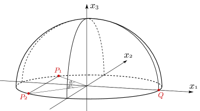
Figure 16. $P_{1}$,$P_{2}$ and $Q$ on the unit hemisphere.

For $1\leq\gamma\leq\left\{\log_{2}\left(\frac{2\pi}{3\arccos{(1/4)}}\right)\right\}^{-1}$, we consider C1. As in the proof of Theorem 5.2(3), we can set $\mu=X=(-\sin\theta,0,\cos\theta)$. Let $S_{X}$ and $S_{P_{1}}$ denote $L_{\gamma}$-dispersion from $X$ and $P_{1}$, respectively. Then,

$$S_{X} =m(\pi/2+\theta)^{\gamma}+2M\{\arccos(1-\cos^{2}\theta(1-\cos\psi))\},$$

$$S_{P_{1}} =m(\pi/2+\theta)^{\gamma}+M\{\arccos(1-2\cos^{2}\theta\sin^{2}\psi)\}.$$

Therefore, $S_{X}<S_{P_{1}}$ is equivalent to

$$\arccos(1-2\cos^{2}\theta\sin^{2}\psi)<2^{1/\gamma}\arccos\{1-\cos^{2}\theta(1-\cos\psi)\}.$$

By setting $\psi=\arccos\{(1-1/2(1-\sin\theta))^{1/2}\}$, this is equivalent to $\gamma<\gamma_{0}(\theta)$ and also $\theta<\theta_{0}(\gamma)$. Thus, if we set $\theta\geq\theta_{0}(\gamma)$, C1 becomes an example of a non-unique intrinsic $L_{1}$-mean of diameter $\theta+\pi/2$.

For C2, $S_{X}<S_{P_{1}}$ is equivalent to $\pi-2\theta<2^{1/\gamma}\arccos(\sin^{2}\theta)$, and we can prove that it becomes a similar example. After scaling by $1/\sqrt{k}$, these examples give the upper bound on $D_{L_{\gamma}}$. ∎

References

- Alexander and Jones (2000) Alexander L, Jones P (2000) Updated precipitation series for the uk and discussion of recent extremes. Atmospheric science letters 1(2):142–150
- Amari (1985) Amari SI (1985) Differential-Geometrical Methods in Statistics. Springer Science & Business Media
- Amari and Nagaoka (2007) Amari SI, Nagaoka H (2007) Methods of Information Geometry. American Mathematical Soc.
- Arjovsky et al (2017) Arjovsky M, Chintala S, Bottou L (2017) Wasserstein GAN 1701.07875
- Ay et al (2017) Ay N, Jost J, Lê HV, Schwachhöfer L (2017) Information Geometry. Ergebnisse der Mathematik und ihrer Grenzgebiete. 3. Folge / A Series of Modern Surveys in Mathematics, Springer
- Bache and Lichman (2013) Bache K, Lichman M (2013) Uci machine learning repository. URL http://archive.ics.uci.edu/ml/
- Belkin and Niyogi (2002) Belkin M, Niyogi P (2002) Laplacian eigenmaps and spectral techniques for embedding and clustering. In: Dietterich TG, Becker S, Ghahramani Z (eds) Advances in Neural Information Processing Systems 14, MIT Press, pp 585–591
- Bengio et al (2013) Bengio Y, Courville A, Vincent P (2013) Representation learning: a review and new perspectives. IEEE Trans Pattern Anal Mach Intell 35(8):1798–1828
- Berman et al (2000) Berman HM, Westbrook J, Feng Z, Gilliland G, Bhat TN, Weissig H, Shindyalov IN, Bourne PE (2000) The protein data bank. Nucleic Acids Res 28(1):235–242
- Bhattacharya and Bhattacharya (2012a) Bhattacharya A, Bhattacharya R (2012a) Nonparametric Inference on Manifolds: With Applications to Shape Spaces. Cambridge University Press
- Bhattacharya and Bhattacharya (2012b) Bhattacharya A, Bhattacharya R (2012b) Nonparametric inference on manifolds: with applications to shape spaces. 2, Cambridge University Press
- Billera et al (2001) Billera LJ, Holmes SP, Vogtmann K (2001) Geometry of the space of phylogenetic trees. Adv Appl Math 27(4):733–767
- Bridson and Haefliger (2011) Bridson MR, Haefliger A (2011) Metric spaces of non-positive curvature, vol 319. Springer Science & Business Media
- Cayton (2005) Cayton L (2005) Algorithms for manifold learning. Univ of California at San Diego Tech Rep 12(1-17):1
- CIESEN et al (2005) CIESEN, FAO, CIAT (2005) Gridded population of the world, version 3 (gpwv3): Population count grid. URL http://dx.doi.org/10.7927/H4639MPP, accessed 16/June/2016.
- Cuturi and Doucet (2014) Cuturi M, Doucet A (2014) Fast computation of wasserstein barycenters. In: International Conference on Machine Learning, jmlr.org, pp 685–693
- De Berg et al (2000) De Berg M, Van Kreveld M, Overmars M, Schwarzkopf OC (2000) Computational geometry. In: Computational geometry, Springer, pp 1–17
- Deza and Deza (2009) Deza MM, Deza E (2009) Encyclopedia of distances. In: Encyclopedia of Distances, Springer, pp 1–583
- Dryden and Mardia (2016) Dryden IL, Mardia KV (2016) Statistical Shape Analysis: With Applications in R. John Wiley & Sons
- Espínola and Fernández-León (2009) Espínola R, Fernández-León A (2009) Cat (k)-spaces, weak convergence and fixed points. Journal of Mathematical Analysis and Applications 353(1):410–427
- Floyd (1962) Floyd RW (1962) Algorithm 97: shortest path. Communications of the ACM 5(6):345
- Gromov (1987) Gromov M (1987) Hyperbolic groups. In: Essays in group theory, Springer, pp 75–263
- Kendall (1984) Kendall DG (1984) Shape manifolds, procrustean metrics, and complex projective spaces. Bull Lond Math Soc 16(2):81–121
- Kendall et al (2009) Kendall DG, Barden D, Carne TK, Le H (2009) Shape and Shape Theory. John Wiley & Sons
- Kendall and Morán (1963) Kendall MG, Morán PA (1963) Geometrical probability. Tech. rep.
- Kendall (1990) Kendall WS (1990) Probability, convexity, and harmonic maps with small image i: uniqueness and fine existence. Proceedings of the London Mathematical Society 3(2):371–406
- Komaki (2006) Komaki F (2006) Shrinkage priors for bayesian prediction. Ann Stat 34(2):808–819
- Lin et al (2011) Lin Y, Lu L, Yau ST (2011) Ricci curvature of graphs. Tohoku Math J 63(4):605–627
- Marron and Alonso (2014) Marron JS, Alonso AM (2014) Overview of object oriented data analysis. Biom J 56(5):732–753
- McCullagh (1986) McCullagh P (1986) Tensor Methods in Statistics. Courier Dover Publications
- Nye (2011) Nye TMW (2011) Principal components analysis in the space of phylogenetic trees. Ann Stat 39(5):2716–2739
- Okabe et al (2009) Okabe A, Boots B, Sugihara K, Chiu SN (2009) Spatial tessellations: concepts and applications of Voronoi diagrams, vol 501. John Wiley & Sons
- Owen and Provan (2011) Owen M, Provan JS (2011) A fast algorithm for computing geodesic distances in tree space. IEEE/ACM Trans Comput Biol Bioinform 8(1):2–13
- Panaretos and Zemel (2018) Panaretos VM, Zemel Y (2018) Statistical aspects of wasserstein distances 1806.05500
- Patrangenaru and Ellingson (2015) Patrangenaru V, Ellingson L (2015) Nonparametric statistics on manifolds and their applications to object data analysis. CRC Press
- Peyré and Cuturi (2018) Peyré G, Cuturi M (2018) Computational optimal transport 1803.00567
- Ramsay and Silverman (2007) Ramsay JO, Silverman BW (2007) Applied Functional Data Analysis: Methods and Case Studies. Springer
- Saul (2003) Saul LK (2003) Think globally, fit locally: Unsupervised learning of low dimensional manifolds. J Mach Learn Res 4:119–155
- Solomon et al (2015) Solomon J, de Goes F, Peyré G, Cuturi M, Butscher A, Nguyen A, Du T, Guibas L (2015) Convolutional wasserstein distances: Efficient optimal transportation on geometric domains. ACM Trans Graph 34(4):66:1–66:11
- Srivastava and Klassen (2016) Srivastava A, Klassen EP (2016) Functional and Shape Data Analysis. Springer Series in Statistics, Springer
- Takatsu (2011) Takatsu A (2011) Wasserstein geometry of gaussian measures. Osaka J Math 48(4):1005–1026
- Tanaka and Komaki (2008) Tanaka F, Komaki F (2008) A superharmonic prior for the autoregressive process of the second-order. J Time Ser Anal 29(3):444–452
- Tenenbaum et al (2000) Tenenbaum JB, de Silva V, Langford JC (2000) A global geometric framework for nonlinear dimensionality reduction. Science 290(5500):2319–2323
- Vallender (1974) Vallender S (1974) Calculation of the wasserstein distance between probability distributions on the line. Theory Probab Appl 18(4):784–786
- Villani (2008) Villani C (2008) Optimal Transport: Old and New. Springer Science & Business Media
- Wang and Marron (2007) Wang H, Marron JS (2007) Object oriented data analysis: Sets of trees 0711.3147
- Yang and Jin (2006) Yang L, Jin R (2006) Distance metric learning: A comprehensive survey. Michigan State Universiy 2(2):4