The MUSIC of Galaxy Clusters II: X-ray global properties and scaling relations

Abstract

We present the X-ray properties and scaling relations of a large sample of clusters extracted from the Marenostrum MUltidark SImulations of galaxy Clusters (MUSIC) dataset. We focus on a sub-sample of 179 clusters at redshift $z\sim 0.11$, with $3.2\times 10^{14}h^{-1}\rm{~{}M_{\odot}}<M_{vir}<2\times 10^{15}h^{-1}\rm{~{}M_{\odot}}$, complete in mass. We employed the X-ray photon simulator PHOX to obtain synthetic Chandra observations and derive observable-like global properties of the intracluster medium (ICM), as X-ray temperature ($T_{X}$) and luminosity ($L_{X}$). $T_{X}$ is found to slightly under-estimate the true mass-weighted temperature, although tracing fairly well the cluster total mass. We also study the effects of $T_{X}$ on scaling relations with cluster intrinsic properties: total ($M_{500}$ and gas $M_{g,500}$ mass; integrated Compton parameter ($Y_{SZ}$) of the Sunyaev-Zel’dovich (SZ) thermal effect; $Y_{X}=M_{g,500}\,\,T_{X}$. We confirm that $Y_{X}$ is a very good mass proxy, with a scatter on $M_{500}-Y_{X}$ and $Y_{SZ}-Y_{X}$ lower than $5\%$. The study of scaling relations among X-ray, intrinsic and SZ properties indicates that simulated MUSIC clusters reasonably resemble the self-similar prediction, especially for correlations involving $T_{X}$. The observational approach also allows for a more direct comparison with real clusters, from which we find deviations mainly due to the physical description of the ICM, affecting $T_{X}$ and, particularly, $L_{X}$.

1 INTRODUCTION

In the last decades, X-ray observations of galaxy clusters have continuously provided us with precious information on their intrinsic properties and components. In particular, the X-ray emission from the diffuse intracluster medium (ICM) has been proved to be a good tracer of both the physics governing the gaseous component and the characteristics of the underlying potential well, basically dominated by the non-luminous, dark matter (see Sarazin, 1986).
A reliable estimate of their total mass represents a fundamental goal of astrophysical and cosmological investigations, as the accurate weighing of clusters is also crucial to use them as cosmological probes, e.g. via number counts (see, e.g. Allen et al., 2011, and references therein). In the X-ray band clusters are very bright sources relatively easy to detect out to high redshifts and constitute therefore a powerful tool to select large samples of objects for cosmology studies. However, the mass determination via X-ray observations is mainly possible for well resolved, regular, nearby galaxy clusters, for which ICM density and temperature profiles are measurable with good precision and the Hydrostatic Equilibrium (HE) hypothesis can be safely applied.
As widely discussed in the literature Rasia et al. (2006); Nagai et al. (2007); Lau et al. (2009); Meneghetti et al. (2010); Suto et al. (2013), the hydrostatic mass can mis-estimate the true total mass by a factor up to $20-30$ percents, due to underlying erroneous assumptions (e.g. on the dynamical state of the system, on the ICM non-thermal pressure support, on the models used to deproject observed density and temperature profiles, or on cluster sphericity).
In many cases, especially at high redshift or for more disturbed, irregular systems, when the hydrostatic X-ray mass cannot be inferred reliably, mass proxies are commonly employed to obtain indirect mass estimates. Scaling relations between global cluster properties can be invoked to this purpose, offering a substitute approach to derive the total mass from other observables, e.g. obtained from the X-ray band or through the thermal Sunyaev Zel’dovich (SZ; Sunyaev & Zeldovich, 1970, 1972) effect.
In fact, the simple scenario of the gravitational collapse, by which gravity is dominating the cluster formation process, predicts a self-similar scaling of basic cluster observables with their mass Kaiser (1986). Observations of galaxy clusters have confirmed the presence of correlations among cluster properties, and with mass, although indicating in some cases a certain level of deviation from the expected self-similar slopes. The main reason for this deviation is that non-gravitational processes on smaller scales (e.g. cooling, dynamical interactions, feedback from active galactic nuclei – AGN –) do take place during the assembly of clusters and have a non-negligible effect on their energy content. In this respect, a remarkable example is represented by the X-ray luminosity–temperature relation, which is commonly observed to be significantly steeper than expected White et al. (1997); Markevitch (1998); Arnaud & Evrard (1999); Ikebe et al. (2002); Ettori et al. (2004); Maughan (2007); Zhang et al. (2008); Pratt et al. (2009).
In order to employ scaling relations to infer masses, also the scatter about the relations has to be carefully considered: the tighter the correlation, the more precise can be the mass estimate. Therefore, investigating the intrinsic scatter that possibly exists for correlation with certain properties is extremely useful in order to individuate the lowest-scatter mass proxy among many observable properties (e.g. Ettori et al., 2012). This is the case, for instance, of the integrated Compton parameter, $Y_{SZ}$, a measure of the thermal SZ signal which has been confirmed to closely trace the cluster total mass by both simulations and observations da Silva et al. (2004); Nagai (2006); Morandi et al. (2007); Bonamente et al. (2008); Comis et al. (2011); Sembolini et al. (2013); Kay et al. (2012); Planck Collaboration (2013). The physical motivation for this is that $Y_{SZ}$ is related to the ICM pressure (integrated along the line of sight), or equivalently to its total thermal energy, and thus to the depth of the cluster potential well. Likewise, another remarkably good candidate is also the X-ray-analog of the $Y_{SZ}$ parameter, $Y_{X}$, which was introduced by Kravtsov et al. (2006) and similarly quantifies the ICM thermal energy by the product of gas mass and spectroscopic temperature. Therefore, $Y_{X}$ correlates strictly with $Y_{SZ}$, but also with total mass, given a fortunate anti-correlation of the residuals in temperature and gas mass.
As widely explored in the literature, numerical hydrodynamical simulations can be as precious as observations in unveiling the effects of a number of physical processes on the global properties and self-similar appearance of galaxy clusters (see, e.g., recent reviews by Borgani & Kravtsov, 2011; Kravtsov & Borgani, 2012). Current hydrodynamical simulations can be further exploited when results are obtained in an observational fashion, which makes the results more directly comparable to real data, e.g. from the X-ray band (e.g. Mathiesen & Evrard, 2001; Gardini et al., 2004; Mazzotta et al., 2004; Rasia et al., 2005; Rasia et al., 2006; Valdarnini, 2006; Kravtsov et al., 2006; Nagai et al., 2007; Jeltema et al., 2008; Biffi et al., 2012; Biffi et al., 2013a, b) or weak lensing (e.g. Meneghetti et al., 2010; Rasia et al., 2012). Under this special condition, projection and instrumental effects, unavoidable in real observations, can be limited and explored for the ideal case of simulated clusters, as the intrinsic properties can be calculated exactly from the simulation.
In return, simulations themselves can take advantage of such technique, as mis-matches between theoretical definitions of observable properties, used in numerical studies, can be overcome (see, e.g., studies on the ICM X-ray temperature by Mazzotta et al., 2004; Valdarnini, 2006; Nagai et al., 2007) and the capability of the implemented physical descriptions to match real clusters can be better constrained (e.g. Puchwein et al., 2008; Fabjan et al., 2010, 2011; Biffi et al., 2013a).
This is the approach we intend to follow in the present work. Specifically, we study the Marenostrum MUltidark SImulations of galaxy Clusters (MUSIC) data-set of cluster re-simulations by means of synthetic X-ray observations obtained with the virtual photon simulator PHOX Biffi et al. (2012). The scope of this analysis is to extend the study carried on by Sembolini et al. (2013) to the X-ray features and scaling relations of the MUSIC clusters, thereby providing a more complete picture of this simulated set with respect to their baryonic properties. In fact, X-ray observables are highly susceptible to the complexity of the ICM physical state (e.g. to its multi-phase structure) and can be more significantly affected by the numerical description of the baryonic processes accounted for in the simulations (particularly cooling, star formation and feedback mechanisms).
The paper is organized as follows.
In Section 2 we present the sub-sample of simulated objects considered for the present study, whereas the generation and analysis of synthetic X-ray observations are described in Section 3. In Section 4 we discuss the main results. Specifically, X-ray observables are analysed and compared to theoretical estimates derived directly from the simulations (Section 4.1). In Section 4.2 we present instead mass-observable correlations (Section 4.2.1, Section 4.2.2, Section 4.2.3), as well as pure X-ray (Section 4.2.4) and mixed X-ray/SZ (Section 4.2.5, Section 4.2.6, Section 4.2.7) scaling relations. These are analysed and discussed with respect to the effects of the observational-like approach, the X-ray temperature determination, the compatibility with the expected self-similar scenario and the comparison against observational and previous numerical findings (Section 4.2.8).
Finally we draw our conclusions in Section 5.

2 Simulated sample of galaxy clusters

The numerical simulations employed in the present work are part of the MUSIC project, in particular of the MultiDark sub-set of re-simulated galaxy clusters (MUSIC-2, see Sembolini et al., 2013).
The MultiDark simulation (MD) is a dark-matter-only N-body simulation performed with the adaptive refinement tree (ART) code Kravtsov et al. (1997), resolved with $2048^{3}$ particles in a $(1h^{-1}\rm{~{}Gpc})^{3}$ volume Prada et al. (2012). The cosmology assumed refers to the best-fit parameters obtained from the WMAP7+BAO+SNI data, i.e. $\Omega_{M,0}=0.27$, $\Omega_{b}=0.0469$, $\Omega_{\Lambda,0}=0.73$, $h_{0}=0.7$, $\sigma_{8}=0.82$ and $n=0.95$ Komatsu et al. (2011).
MUSIC-2 re-simulated clusters: a complete, mass selected, volume limited sample of 282 clusters has been extracted from a low resolution ($256^{3}$ particles) run of the MD simulation. Namely, it comprises all the systems in the $(1h^{-1}\rm{~{}Gpc})^{3}$ volume with virial mass larger than $10^{15}h^{-1}\rm{~{}M_{\odot}}$ at redshift $z=0$.
Each one of the identified systems has been then re-simulated with higher resolution and including hydrodynamics, within a radius of $6h^{-1}\rm{~{}Mpc}$ from the center of each object at $z=0$. Initial conditions for the re-simulations were generated with the zooming technique by Klypin et al. (2001). The re-simulations were performed with the TreePM/SPH parallel code GADGET Springel et al. (2001); Springel (2005), including treatments for cooling, star formation and feedback from SNe winds Springel & Hernquist (2003). The final mass resolution for these re-simulations is $m_{DM}=9.01\times 10^{8}h^{-1}\rm{~{}M_{\odot}}$ and $m_{gas}=1.9\times 10^{8}h^{-1}\rm{~{}M_{\odot}}$, respectively.
This permitted to obtain a huge catalog of cluster-like haloes, namely more than five hundreds objects more massive than $10^{14}h^{-1}\rm{~{}M_{\odot}}$ at redshift zero.
Snapshots corresponding to 15 different redshifts have been stored between $z=9$ and $z=0$.

2.1 The simulated data-set

The sub-sample of re-simulated galaxy clusters for which we want to analyse X-ray properties is selected from the MUSIC-2 data-set employed in the work presented by Sembolini et al. (2013).
For the present analysis, we focus in particular on one snapshot at low redshift, i.e. z=0.11. This redshift corresponds to one of the first time records of the simulation output earlier than $z=0$ and is suitable to investigate cluster properties in a relatively recent epoch with respect to the early stages of formation.
Precisely, we select all the clusters matching the mass completeness of the MUSIC-2 dataset at this redshift (see Sembolini et al., 2013), i.e. $M_{vir}(z=0.11)>7.5\times 10^{14}h^{-1}\rm{~{}M_{\odot}}$. Additionally, we also enlarge the sub-sample in order to comprise all the progenitors at $z=0.11$ of the systems with virial masses above the completeness mass limit at $z=0$ ($M_{vir}(z=0)>8.5\times 10^{14}h^{-1}\rm{~{}M_{\odot}}$). This practically extends the $z=0.11$ selection towards the intermediate-mass end.
As a result, we obtain a volume-limited sample of 179 clusters that is complete in mass at $z=0.11$, with $M_{vir}(z=0.11)$ spanning the range $[3.2-20]\times 10^{14}h^{-1}\rm{~{}M_{\odot}}$.

3 The synthetic X-ray observations with PHOX

Synthetic X-ray observations of the galaxy clusters of the selected sample have been performed by means of the X-ray photon simulator PHOX (see Biffi et al., 2012, for an extensive presentation of the implemented approach).
The cube of virtual photons associated to each cluster box has been generated for the simulated snapshot at redshift $z=0.11$.
For each gas element in the simulation, X-ray emission has been derived by calculating a theoretical spectral model with the X-ray-analysis package XSPEC Arnaud (1996). In particular, we assumed the thermal APEC model Smith et al. (2001), and also combined this with an absorption model, WABS Morrison & McCammon (1983), in order to mimic the suppression of low-energy photons due to Galactic absorption. To this purpose, the equivalent hydrogen column density parameter has been fixed to the fiducial value of $N_{H}=10^{20}cm^{-2}$. Temperature, total metallicity and density of each gas element, required to calculate the spectral emission model, have been directly obtained from the hydrodynamical simulation output.
At this stage, fiducial, ideal values for collecting area and observation time have been assumed, namely $A_{fid}=1000\rm{~{}cm}^{2}$ and $\tau_{exp,fid}=1\rm{~{}Ms}$.
For the geometrical selection we have considered a cylinder-like region enclosed by the $R_{500}$ radius around each cluster. The radius $R_{500}$ is here defined as the radius encompassing a region with an overdensity of $\Delta_{cr}=500$, with respect to the critical density of the Universe, and in the following we will always use this definition when referring to $R_{500}$. This choice is motivated by our intention of comparing against the majority of the observational and numerical works in literature, which commonly adopt the same overdensity. As for the projection, we consider a line of sight (l.o.s.) aligned with the z-axis of the simulation box.
Finally, we assume a realistic exposure time of $100\rm{~{}ks}$ and perform synthetic observations for the ACIS-S detector of Chandra. This is done with PHOX Unit-3, by convolving the ideal photon lists extracted from the selected regions with the ancillary response file (ARF) and the redistribution matrix file (RMF) of the ACIS-S detector.
Given the adopted cosmology, the $17^{\prime}\times 17^{\prime}$ field of view (FoV) of Chandra corresponds at our redshift to a region in the sky of $2062.44\rm{~{}kpc}$ per side (physical units), which would not comprise the whole $R_{500}$ region for the majority of the clusters in the sample. Nevertheless, one can always assume to be ideally able to entirely cover each cluster with multiple-pointing observations and therefore we profit from the simulation case to extract X-ray properties from within $R_{500}$ for all the objects.

3.1 X-ray analysis of Chandra synthetic spectra

The synthetic Chandra spectra generated with PHOX have been re-grouped requiring a minimum of 20 counts per energy bin. Spectral fits of the synthetic Chandra spectra, corresponding to the $R_{500}$ region of each cluster, have been performed over the $0.5-10\rm{~{}keV}$ energy band by using XSPEC and adopting an absorbed (WABS), thermally-broadened, APEC model, which takes into account a single-temperature plasma to model the ICM emission. In the fit, parameters for galactic absorption and redshift have been fixed to the original values assumed to produce the observations, while the other parameters were allowed to vary.
For all the clusters in the sample, the best-fit spectral model generally indicates a very low value of the total metallicity of the plasma. This result is simply reflecting the treatment of the star formation and metal production in the original input simulations, which does not follow proper stellar evolution and injection of metal yields according to proper stellar life-times.
We note that, even though the ICM in the clusters is most likely constituted by a multi-phase plasma, the single-temperature fit results overall in reasonable estimations, for all the clusters in our sample, as confirmed by the $\chi^{2}$ statistics (see Fig. 14 in Appendix A). From the distribution of the reduced-$\chi^{2}$ values, we have in fact $\chi^{2}<1.2$ for $\sim 70\%$ of the clusters in the sample.

4 Results

In this Section we present the X-ray properties and scaling relations of the 179 galaxy clusters in the sample, at $z=0.11$, obtained from Chandra synthetic observations.

4.1 X-Ray properties of the massive haloes

Two interesting, global X-ray properties that we can directly extract from spectral analysis are the luminosity and temperature of the ICM within the projected $R_{500}$.

4.1.1 The X-ray luminosity

From the theoretical best-fit model to the synthetic data, we calculate X-ray luminosities for the sample clusters in the entire $0.5-10\rm{~{}keV}$ band, as well as in the Soft and Hard X-ray bands, i.e. $0.5-2\rm{~{}keV}$ and $2-10\rm{~{}keV}$, respectively (rest frame energies).
Furthermore, we extrapolate the total X-ray luminosity to the maximum energy band defined by the Chandra response matrix, i.e. $0.26-12\rm{~{}keV}$ ($0.28-13.3\rm{~{}keV}$ rest frame). Hereafter, we will refer to this quantity as the “bolometric” X-ray luminosity.
In Fig. 1 we show the cumulative luminosity function built from the “bolometric” X-ray luminosity within $R_{500}$ of all the clusters in the sample, ${\rm d}{N}(>L_{X})/{\rm d}{Vol}$ (for a volume corresponding to the simulation box volume)

Figure 1: Cumulative luminosity function for the sample of clusters.

4.1.2 The X-ray temperature

From the analysis of the Chandra synthetic spectra, we also measure the projected mean temperature within $R_{500}$. All the clusters of the sample have temperatures $T_{X}>2\rm{~{}keV}$. This temperature, usually referred to as “spectroscopic” temperature can be compared to the temperature estimated from the simulation as

$$T_{w}=\frac{\Sigma_{i}w_{i}T_{i}}{\Sigma_{i}w_{i}},$$ (1)

where the sums are performed over the SPH particles in the considered region of the simulated cluster. The temperature associated to the single gas particle ($T_{i}$) is computed taking into account the multi-phase gas description following the model by Springel & Hernquist (2003).
The weight $w$ in Eq. 1 changes according to different theoretical definitions.
As commonly done, we consider:

• the mass-weighted temperature, $T_{mw}$, where $w_{i}=m_{i}$;

• the emission-weighted temperature, $T_{ew}$, where the emission is $\sim\rho^{2}\Lambda(T)\sim\rho^{2}\sqrt{T}$ (the cooling function can be approximated by $\Lambda(T)\sim\sqrt{T}$ for dominating thermal bremsstrahlung) and therefore $w_{i}=m_{i}\rho_{i}\sqrt{T_{i}}$;

• the spectroscopic-like temperature, $T_{sl}$, where $w_{i}=m_{i}\rho_{i}T_{i}^{-3/4}$ (which was proposed by Mazzotta et al., 2004, as a good approximation of the spectroscopic temperature for systems with $T\gtrsim 2-3\rm{~{}keV}$).

While computing the emission-weighted and spectroscopic-like temperatures, we apply corrections to the particle density that account for the multi-phase gas model adopted (consistently to what is done while generating the X-ray synthetic emission) and we exclude cold gas particles, precisely those with temperatures $<0.5\rm{~{}keV}$.
Among the aforementioned theoretical estimates, the mass-weighted temperature is the value that most-closely relates to the mass of the cluster, directly reflecting the potential well of the system.

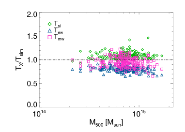
Figure 2: Relations between the X-ray-derived temperature, obtained from spectral fitting of the synthetic spectra in the (0.5-10) keV band, and the different theoretical definitions of temperature estimated directly from the simulation: $T_{mw}$ (mass-weighted, magenta squares), $T_{ew}$ (emission-weighted, blue triangles), $T_{sl}$ (spectroscopic-like, green diamonds). Temperature ratios are plotted as function of the cluster mass within $R_{500}$ ($M_{500}$).

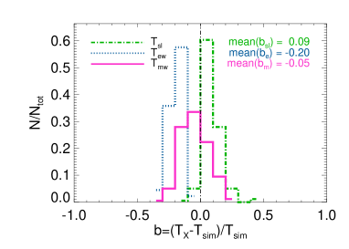
Figure 3: Distribution of the deviations of the X-ray temperature from the simulation estimates, according to the three theoretical definitions: $T_{mw}$ (solid), $T_{ew}$ (dotted), $T_{sl}$ (dash-dotted). Colors as in Fig. 2. The distributions are normalized to the total number of clusters in the sample. Mean value and standard deviation of each distribution are: $(0.09\pm 0.07)$ for $T_{sim}\equiv T_{sl}$; $(-0.20\pm 0.05)$ for $T_{sim}\equiv T_{ew}$; $(-0.05\pm 0.10)$ for $T_{sim}\equiv T_{mw}$.

Nevertheless, the various other ways of weighting the temperature for the gas emission (such as $T_{ew}$ or $T_{sl}$) have been introduced in order to better explore the X-ray, observable properties of simulated galaxy clusters and to ultimately compare against real observations. Differences among these definitions and their capabilities to match the observed X-ray temperature have been widely discussed in the literature (e.g. Mathiesen & Evrard, 2001; Mazzotta et al., 2004; Rasia et al., 2005; Valdarnini, 2006; Nagai et al., 2007).
From the comparison shown in Fig. 2, we also remark the differences existing among the theoretical estimates and the expected spectroscopic temperature $T_{X}$, derived from proper spectral fitting. The spectroscopic temperature refers, in this case, to the region within the projected $R_{500}$, which might introduce deviations due to substructures lying along the l.o.s.. Despite this, we expect it to be fairly consistent to the global, 3D value, given the large region considered.
In Fig. 2, the ratio $T_{X}/T_{sim}$ is presented as a function of the true cluster mass within $R_{500}$, $M_{500}$.
Comparing to the 1:1 relation (black, dot-dashed line in the Figure), we note that there are discrepancies among the values. Overall, we conclude from this comparison that $T_{X}$ tends to be generally higher than the value of $T_{sl}$. Also, in perfect agreement to the findings of previous works (e.g. Mazzotta et al., 2004), the spectroscopic temperature $T_{X}$ is on average lower than the emission-weighted estimate.
It’s interesting to notice, that in our case the discrepancy between $T_{X}$ and the true, dynamical temperature of the clusters, $T_{mw}$, is smaller than the deviation from either emission-weighted or spectroscopic-like temperatures.
Nonetheless, with respect to the mass-weighted value, we find that $T_{X}$ tends to be slightly biased low. On one hand, this under-estimation of the true temperature by the X-ray-derived measurement might be ameliorated via a further exclusion a posteriori of cold, gaseous substructures in the ICM. On the other hand, a complexity in the thermal structure of the ICM can persist (for instance, a broad temperature distribution, or a significant difference in the temperatures of the two most prominent gas phases) and eventually affect the resulting X-ray temperature, especially when a single temperature component is fitted to the integrated spectrum.
As a test, we checked for the dependency of the bias on the $\chi^{2}_{red}$ of the fit and found that there is a mild correlation (see Fig. 14 in Appendix A). Precisely, to higher $\chi^{2}_{red}$ values of the one-temperature spectral fit, correspond on average lower $T_{X}/T_{mw}$ ratios (and similarly for $T_{X}/T_{ew}$). Comparing $T_{X}$ to $T_{sl}$ this effect basically disappears, confirming that they are almost equally sensitive to the complexity of the ICM thermal distribution.
The observed under-estimation of the true temperature by $T_{X}$ is in agreement with findings from, e.g., early studies using mock X-ray observations of simulated clusters by Mathiesen & Evrard (2001), but there is instead some tension with respect to other numerical studies (e.g. Nagai et al., 2007; Piffaretti & Valdarnini, 2008). Nevertheless, as reported also by Kay et al. (2012), who found results consistent with what observed in MUSIC clusters, the discrepancy might be due to the additional exclusion of resolved cold clumps in the X-ray analysis.
In fact, for the set of MUSIC clusters, we observe that a two-temperature model would generally improve the quality of the fit (especially for the objects where the single-temperature fit provides $\chi^{2}_{red}>1.2$), better capturing the local multi-phase nature of the gas. However, the best-fit hotter component tends to over-estimate the mass-weighted temperature, introducing even in this case a significant bias in the results. Moreover, this increases the overall scatter, particularly for colder, low-mass systems, where it is more difficult to distinguish between the two temperature components. Therefore, we decide to consider throughout the following analysis the results from the single-temperature best-fit models.
Another, more quantitative, way of comparing the deviations of $T_{sl}$, $T_{ew}$ and $T_{mw}$ from $T_{X}$ is by confronting the distributions of the bias, defined as:

$$b=\frac{T_{X}-T_{sim}}{T_{sim}},$$ (2)

shown in Fig. 3.
From this we clearly observe that the distribution of $b$ for $T_{sim}\equiv T_{mw}$ shows the best agreement with the 1:1 relation, although it is not symmetrical and rather biased toward negative deviations. This corresponds to an average under-estimation by $T_{X}$ of $\sim 5$ percent, over the all sample. More specifically, we find that for almost $\sim 67\%$ of the clusters considered $T_{X}$ under-estimates the true temperature of the system.
Emission-weighted and spectroscopic-like temperatures suggest instead more extreme differences and narrower distributions. $T_{ew}$ indicates a more significant mis-match with the X-ray value, which tends to be smaller by a factor of $\sim 20\%$, with little dispersion. $T_{sl}$ is instead closer to the X-ray temperature, although the distribution of the deviations is slightly biased to positive values of $b$, indicating a typical over-estimation by $T_{X}$ of a few percents. The mean value of each bias distribution is reported in the legend of Fig. 3.

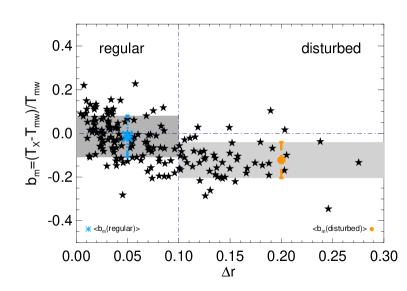
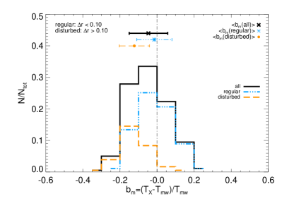
Figure 4: Left panel: Dependence of the temperature bias ($b_{m}=(T_{X}-T_{mw})/(T_{mw})$) on the dynamical state of the cluster, quantified by the center-of-mass off-set ($\Delta r$). The dot-dashed vertical line marks the threshold chosen to separate regular clusters from disturbed ones. In each region of the plot the mean value of the bias $b_{m}$ and standard deviation are marked with a symbol (blue asterisk for regular clusters, orange filled circle for disturbed ones) and a shaded area. Right panel: The distribution of the bias $b_{m}$ is reported for the complete sample (black, solid line) and the regular (blue, dot-dot-dot-dashed line) and disturbed (orange, dashed line) sub-sets. Also, the mean values, with 1-$\sigma$ errors, are reported for the three cases (black x, blue asterisk, orange filled circle, respectively).

4.1.3 Dependence of the temperature bias on the dynamical state

In order to investigate further the bias in the temperature estimation, we concentrate particularly on the bias between spectroscopic and mass-weighted values, i.e. $b_{m}=(T_{X}-T_{mw})/(T_{mw})$ (see Eq. 2), and explore its relation to the global, intrinsic state of the cluster. To this scope, we calculate from the simulations the center-of-mass off-set, defined as

$$\Delta r=\frac{\|r_{\delta}-r_{cm}\|}{R_{vir}},$$ (3)

namely the spatial separation between the maximum density peak ($r_{\delta}$) and the center of mass ($r_{cm}$), normalized to the cluster virial radius ($R_{vir}$). The choice to adopt this value to discriminate between regular and disturbed clusters is related to the search for a quantity able to describe the intrinsic state of the cluster, taking advantage of the full three-dimensional information available in simulations. The threshold adopted to divide the clusters into two sub-samples is the fiducial value of $\Delta r_{th}=0.1$ (see, e.g., D’Onghia & Navarro, 2007). This represents an upper limit in the range of limit values explored in the literature Macciò et al. (2007); Neto et al. (2007); D’Onghia & Navarro (2007); Knebe & Power (2008). In our case, given the presence of the baryonic component, we decide in fact to allow for a less stringent criterion (see also Sembolini et al., 2013).
In Fig. 4 we show the results of this test. The relation between observed bias and $\Delta r$ is shown in the left panel of the Figure. The vertical dashed line marks the separation threshold between regular and disturbed clusters. We note that there is indeed a dependence of the $T_{X}-T_{mw}$ bias on the dynamical state of the cluster, with a general tendency for $b_{m}$ to increase with increasing level of disturbance, quantified by the center-of-mass off-set. More specifically, it is more negative for higher values of $\Delta r$. The filled circle and asterisk, and shaded areas, corresponding to the mean values and standard deviations for the two subsamples, show indeed that the bias distribution is centered very close to zero for the regular clusters, while a more significant off-set is evident for the disturbed sub-sample. The bias distributions for the two subsamples are shown more clearly in the right panel of Fig. 4 and compared to the global distribution. We note that, the bias calculated for the entire sample is basically dominated by the regular clusters, which constitute the majority of the haloes, given the threshold value adopted for $\Delta r$. In particular, we find that for regular clusters $T_{X}$ approximates to a few percents, on average, the true temperature of the cluster: $<b_{M}(regular)>=-0.01\pm 0.01$. The disturbed clusters, instead, are characterised by $<b_{M}(disturbed)>=-0.12\pm 0.01$, indicating a stronger under-estimation.
Despite the difference in the mean values, we remark that the distributions of the two populations are quite broad with respect to the bias, as quantified by the standard deviations and shown also in Fig. 4 ($\sigma_{b_{m}}(regular)=0.10$ and $\sigma_{b_{m}}(disturbed)=0.08$).

4.2 Global scaling relations

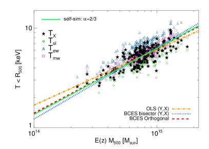
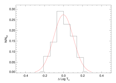
Figure 5: Left: Temperature-mass relation. Open symbols refer to the three standard definitions of temperature used in simulations: $T_{mw}$ (magenta squares), $T_{ew}$ (blue triangles), $T_{sl}$ (green diamonds). Black stars refer to the X-ray temperature, $T_{X}$, extracted from the synthetic spectra in the (0.5-10) keV band. Over-plotted in orange the (OLS) best-fit relation for the $T_{X}-M_{500}$ relation. For comparison, we also report the Bisector and Orthogonal best-fit curves (as in the legend) and the self-similar line, normalized to the data at $7.5\times 10^{14}\rm{~{}M_{\odot}}$, in mass. Right: distribution of the residuals in the $T_{X}-M_{500}$ relation (in ${\rm Log}T_{X}$).

In this Section we focus on cluster global scaling relations. We consider correlations among X-ray quantities measured from the synthetic PHOX observations (e.g. $L_{X}$, $T_{X}$), properties estimated from the thermal SZ signal and intrinsic quantities obtained from the numerical, hydrodynamical simulation data directly.
Also, we aim to compare our findings with both current observational results and theoretical expectations from the gravity-dominated scenario of cluster self-similarity.
In this simplified model, the gravitational collapse giving birth to clusters of galaxies determines entirely the global scaling of the system observable properties. Precisely, the gas is assumed to be heated by the gravitational process only, therefore depending uniquely on the scale set by the system total mass (i.e. by the depth of its potential well), and on the redshift (see Kaiser, 1986). Under these assumptions, power law correlations for each set of observables (Y,X) are expected, namely

$${\rm Y}=C\,({\rm X})^{\alpha},$$ (4)

where $C$ and $\alpha$ are the normalization and the slope of the relation, respectively. Throughout the following, we fit the data with linear relations in the Log-Log plane of the general form

$${\rm Log(Y)}=B+\alpha{\rm Log(X)},$$ (5)

with $B={\rm Log}C$.
The slope and the normalization are recovered via a minimization of the residuals to the best-fit curve (further details on the minimization method adopted will be provided on a case-by-case basis, in the following sections).
Under this formalism, we also calculate the scatter in the Y variable as

$$\sigma_{{\rm LogY}}=\left[\frac{\Sigma_{i=1}^{N}[{\rm Log}({\rm Y_{i}})-(B+\alpha{\rm Log}({\rm X_{i}}))]^{2}}{N-2}\right]^{1/2},$$ (6)

where $N$ is the number of data points (for our analysis this is $N=179$, i.e. the number of clusters in the sample).

4.2.1 Relation between temperature and mass

Here we discuss the relation between temperature and total mass for the subsample of the MUSIC-2 clusters analysed in this work. This is displayed in the left panel of Fig. 5.
The differences that appear while comparing the spectroscopic temperature $T_{X}$ to $T_{mw}$, $T_{ew}$ and $T_{sl}$, basically carry the imprints of the differences existing among the three theoretical estimates of temperature calculated directly from the simulations (see Fig. 5, left panel). Although a shift in temperatures is evident for the different data-sets in Fig. 5 (left panel), we note that for none of them the spread in temperature shows any strong dependence on mass.
Regarding $T_{X}$, we observe that the observational-like temperatures obtained with PHOX appear to be slightly more dispersed than the theoretical values. This might reflect some contamination due to substructures residing along the line of sight and within the projected $R_{500}$, as well as the effect of single-temperature spectral fitting. Even though not major, an increase in scatter and in deviation from self-similarity is also expected as an effect of a more observational-like analysis.
Nevertheless, the overall good correlation between mass and X-ray temperature ensures that the latter behaves as a good tracer of the mass of our clusters, even up to $R_{500}$. This is particularly interesting as the temperature is derived from the cluster X-ray emission, while the mass considered here is the true mass calculated from the simulation.
As a step further, we recover the best-fit relation between the spectroscopic temperature $T_{X}$ and $M_{500}$. As in Eq. 5, we fit the data in the Log-Log plane using the functional form

$${\rm Log}(T_{X})={\rm Log}(C)+\alpha{\rm Log}(E(z)\,M_{500}),$$ (7)

in order to recover slope and normalization of the $T_{X}-M_{500}$ scaling law.
In Eq. 7 (and hereafter), the function $E(z)^{2}=\Omega_{M,0}(1+z)^{3}+\Omega_{\Lambda}$ accounts for the redshift and the cosmology assumed.
In this case, we proceed with a simple ordinary least squares (OLS) minimization method to calculate the slope and normalization of the relation, since the mass is here the intrinsic, true value obtained from the simulation and therefore it should be treated as the “independent” variable. As a result, we find a shallower slope ($\alpha=0.56\pm 0.03$) than predicted by the self-similar model ($\alpha_{self-sim}=2/3$). On the one hand, this shallower dependence might reflect the tendency of $T_{X}$ to under-estimate the true temperature of the system. This is consistent, e.g., with results from numerical studies by Jeltema et al. (2008). On the other hand, the minimization method itself could induce differences in the results, especially when some intrinsic scatter in the relation is present. Indeed, we find a steeper slope when the residuals on both variables are minimized, e.g. via the bisector – $\alpha=0.72\pm 0.03$ – or orthogonal – $\alpha=0.65\pm 0.04$ – approaches (Bivariate Correlated Errors and intrinsic Scatter – BCES) . For the purpose of comparison, we report in Fig. 5 (left panel) the best-fit curves for all the three methods, as well as the self-similar relation (normalized to the data at $7.5\times 10^{14}~{}h^{-1}\rm{~{}M_{\odot}}$, in mass).
For this sample, the scatter in ${\rm Log}T_{X}$ with respect to the best-fit relation is some percents, namely $\sigma_{{\rm Log}T_{X}}\sim 0.07$, calculated according to Eq. 6.
In the right-hand-side panel of Fig. 5 we show the distribution of the OLS residuals for the $T_{X}-M_{500}$ relation, in ${\rm Log}T_{X}$. This can be fitted by a Gaussian function, centered on zero and with standard deviation $\sigma\sim 0.10$.

4.2.2 Relation between luminosity and mass

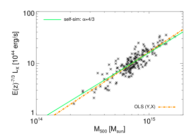
Figure 6: Luminosity–mass relation for the total X-ray band covered by the Chandra detector response, to which we refer as “bolometric” X-ray luminosity. The over-plotted dot-dashed, orange curve is the (OLS) best-fit relation to the data, while the solid green line marks the self-similar relation, normalized to the data at $7.5\times 10^{14}~{}h^{-1}\rm{~{}M_{\odot}}$, in mass.

As well as the temperature, also the X-ray luminosity ($L_{X}$) is expected to scale with the cluster mass (see, e.g. Giodini et al., 2013, for a recent review on cluster scaling relations). Therefore, we show here the $L_{X}-M_{500}$ relation for our clusters, within $R_{500}$. In the case of luminosity, we expect the signature of gas physics to play a major role, introducing both a deviation from self-similarity and a larger scatter. Indeed, the X-ray emission of the ICM is much more sensitive to its thermal state, e.g. to the multi-temperature components of the gas and to substructures. Furthermore, the implementation of the complex processes governing the gas physics, such as cooling, metal enrichment and feedback mechanisms, can certainly have a non-negligible effect.
Indeed, we observe a steeper correlation than expected and a larger scatter with respect to the temperature–mass relation, $\sigma_{{\rm Log}L_{X}}\sim 0.11$ (Section 4.2.1). The best-fit slope obtained from the OLS minimization method is $\alpha\sim 1.45\pm 0.05$, with self-similarity predicting $\alpha_{self-sim}=4/3$. Even though in the same direction, this deviation is however less prominent than for real data (e.g. Maughan, 2007; Arnaud et al., 2010).
In Fig. 6, we display the relation and the best-fit curve. For the purpose of comparison, we also show the self-similar line, normalized in mass to the same pivot used for the best-fit, i.e. $7.5\times 10^{14}~{}h^{-1}\rm{~{}M_{\odot}}$.

4.2.3 Correlations with $Y_{X}$

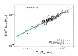
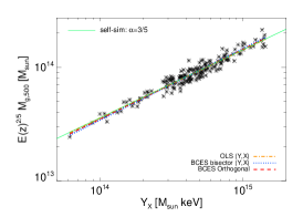
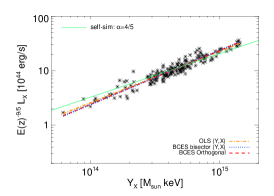
Figure 7: $M_{500}-Y_{X}$ (left), $M_{g,500}-Y_{X}$ (middle) and $L_{X}-Y_{X}$ (right) scaling relations. Best-fit lines for the various approaches are reported as in the legend. As a comparison, we also over-plot the self-similar predicted curve (solid, green), normalized to the data at $Y_{X}=5\times 10^{14}\rm{~{}M_{\odot}}\rm{~{}keV}$.

Additionally, it is interesting to address the effects of the measured X-ray temperature with respect to theoretical, intrinsic quantities inferred directly from the simulations. In particular, we report on the correlations between the total and the gas mass of the clusters, enclosed within $R_{500}$ ($M_{500}$ and $M_{g,500}$, respectively), and the $Y_{X}$ parameter (introduced by Kravtsov et al., 2006), defined as

$$Y_{X}=M_{g}T_{X}.$$ (8)

$Y_{X}$ basically quantifies the thermal energy of the ICM, and we evaluate it for the cluster region within $R_{500}$.
The $M_{g,500}-Y_{X}$ and $M_{500}-Y_{X}$ relations are shown in the left and middle panels of Fig. 7. Here, we employ the X-ray spectroscopic temperature $T_{X}$ but still use the true total ($M_{500}$) and gas ($M_{g,500}$) mass of the simulated clusters, with the sole purpose of calibrating the scaling relations and discerning the effects due to the X-ray (mis-)estimate of the ICM temperature.
We confirm that, despite the complexity of the ICM thermal structure, the estimate of temperature derived from X-ray analysis does not influence majorly the shape of the relation with mass and rather preserves the tight dependence. The slope of both relations ($0.60\pm 0.01$ and $0.58\pm 0.01$, respectively) is very close to the self-similar value ($\alpha_{\rm self-sim}=3/5$) and the scatter in the ${\rm Log}M$ is only about 4 per cent.
The $L_{X}-Y_{X}$ scaling relation (right panel in Fig. 7) shows a steeper ($\alpha\sim 0.94\pm 0.02$) dependence than expected from self-similarity ($\alpha_{\rm self-sim}=4/5$). Even in this case, given the expected good correlation between $Y_{X}$ and the system mass, as well as between temperature and mass, we can ascribe both the larger scatter ($\sigma_{{\rm Log}L_{X}}\sim 0.08$, i.e. a factor of $\sim 2$ larger than in $M_{g,500}-Y_{X}$ and $M_{500}-Y_{X}$) and the deviation from the theoretical self-similar model to the $L_{X}$ observable. Higher values of luminosity for a certain mass can also be affected by the choice of considering the whole region within $R_{500}$, not excluding the innermost part.
Indeed, we find an overall good agreement if compared to similar observational analyses (see, e.g., Maughan, 2007; Pratt et al., 2009). Nonetheless, this MUSIC-2 sub-sample, sampling the most massive clusters, shows a behaviour slightly closer to self-similarity with respect to the observations.

4.2.4 A pure X-ray scaling relation: $L_{X}-T_{X}$

As a further step, we investigate the relation between X-ray luminosity and spectroscopic temperature, within $R_{500}$ (projected radius), for the sample of clusters.
As described in Section 4.1.1, the X-ray luminosity has been obtained from the best-fit of the synthetic Chandra (ACIS-S) spectra generated with the PHOX simulator, for: 0.5-2 $\rm{~{}keV}$ (soft X-ray band, SXR), 2-10 $\rm{~{}keV}$ (hard X-ray band, HXR) and for the total band covered by the ACIS-S detector response (“bolometric” X-ray luminosity). The $L_{X}-T_{X}$ for the three aforementioned energy bands is shown in Fig. 8.

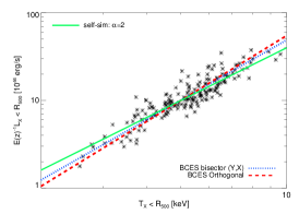
Figure 8: Luminosity–temperature relation for the soft (left panel), hard (middle panel) and “bolometric” (right panel) X-ray band. Right panel: the best-fit lines for the Bisector and Orthogonal methods are marked as in the legend, as well as the self-similar curve (green, solid), normalized to the data at the pivot temperature $5\rm{~{}keV}$.

In order to study the luminosity–temperature scaling law more quantitatively, we perform a linear fit to the $L_{X}-T_{X}$ relation in the Log-Log plane, in order to find the slope, $\alpha$, and normalization, $C$, of the best-fit relation.
Here the functional form in Eq. 5 reads:

$${\rm Log}(E(z)^{-1}\,L_{X})={\rm Log}(C)+\alpha{\rm Log}(T_{X}/T_{0}),$$ (9)

where $L_{X}$ is given in units of $10^{44}\rm{~{}erg/s}$, as well as the normalization $C$, and we assume $T_{0}=5\rm{~{}keV}{}$.
For the purpose of comparison, we recall the self-similar expectation for the luminosity–temperature relation:

$$E(z)^{-1}L\propto T^{2}.$$ (10)

The resulting slope and normalization are sensitive to the method adopted to minimize the residuals, so that a cautious interpretation of the two observables involved in the relations is recommended. We notice that, in the particular case of the $L_{X}-T_{X}$ relation, we might interpret the luminosity as the “dependent” variable and the temperature as the “independent” one, being the latter closely related to the total mass of the cluster (see Fig. 5 and discussion in Section 4.2.1) and therefore tracing an intrinsic property of the system. Under this assumption, the standard OLS method, minimizing only the residuals in the luminosity, would suggest a shallow relation, quite close to the self-similar prediction, with $\alpha=2.08\pm 0.07$.
Nevertheless, a more careful approach to find the best-fit slope consists in a minimization procedure that accounts for both the residuals in $L_{X}$ and $T_{X}$, without any stringent assumption on which variable has to be treated as (in)dependent. Therefore, we apply here the linear regression BCES method, focusing on the Bisector (Y,X) and Orthogonal modifications Isobe et al. (1990); Akritas & Bershady (1996). Both methods are in fact robust estimators of the best-fit slope and provide us with more reliable results than the OLS approach.
For the present analysis, the best-fit values, with their 1-$\sigma$ errors, and the scatter (see Eq. 6) are listed in Table 3. We highlight that the scatter of the relation for this MUSIC-2 subsample is lower ($\sigma_{{\rm LogL_{X}}}\sim 0.11$), with respect to what is usually found when the relation is calculated for a density contrast $\Delta=500$ (see both numerical and observational studies on the $L_{X}-T_{X}$ relation, e.g. Ettori et al., 2004; Maughan, 2007; Pratt et al., 2009; Biffi et al., 2013a, b).
Between the two methods employed, as already pointed out in previous works, the Orthogonal BCES provides a steeper best-fit relation to the data than the Bisector (Y,X) method. Nonetheless, the slope of the relation for the MUSIC-2 clusters is found to be in general shallower, and in slightly better agreement to the self-similar prediction, than often observed at cluster scales (e.g. White et al., 1997; Markevitch, 1998; Arnaud & Evrard, 1999; Ikebe et al., 2002; Ettori et al., 2004; Maughan, 2007; Zhang et al., 2008; Pratt et al., 2009). Here, we notice that the relation is mainly constrained in the high-temperature envelope of the $L_{X}-T_{X}$ plane (for all the clusters $T_{X}>2\rm{~{}keV}$) and we would rather expect a larger statistics in the low-temperature region to introduce a larger deviation from the theoretical expectation. Indeed, a remarkable steepening of the relation is observed especially at galaxy-group scales (or equivalently, for systems with temperatures $<2-3\rm{~{}keV}$), even though this is still a very debated issue (e.g. Ettori et al., 2004; Eckmiller et al., 2011). In agreement with our findings, previous studies indicate a possibly shallower slope that approaches the self-similar expectation for very hot systems (e.g. Eckmiller et al., 2011), which would be the case for the majority of our clusters (see, e.g., Fig. 8, where only 4 objects have $2\rm{~{}keV}<T_{X}<3\rm{~{}keV}$).
In general, the limitations related to the description of the baryonic physics acting in their central region strongly affect the final appearance of simulated clusters, which still fail to match some observational features. Among these, the $L_{X}-T_{X}$ surely represents a critical issue. Certainly, an incomplete description of feedback processes (e.g. from AGN), turbulence (see, e.g. Vazza et al., 2009) and galaxy evolution can weaken the departure of simulated clusters from the theoretical, gravity-dominated scenario and consequently augment the gap between cluster simulations and observations (e.g. Borgani & Kravtsov, 2011, for a recent review).
In the case of observed galaxy clusters, in fact, the deviation from the theoretical expectation is often definitely more striking than what is observed for our simulated sample.
As a final remark, we note that the steepening of the MUSIC $L_{X}-T_{X}$ relation can also possibly point to the combination of two effects: the effect of temperature under-estimation and the possible over-estimation of luminosity, artificially increased in the center because of the incomplete feedback treatment. To this, also the choice of not removing the core from the current analysis can additionally contribute and further investigations in this direction will be worth a separate, dedicated study.

4.2.5 Comparison to SZ-derived properties

We study here correlations between properties of clusters derived from both X-ray synthetic observations and estimates of the SZ signal, in order to build mixed scaling relations for the sample of MUSIC-2 clusters analysed. Both approaches, in fact, allow us to investigate in a complementary way the properties of the hot diffuse ICM and to assess the effects of the baryonic physical processes on the resulting global features (e.g. McCarthy et al., 2003; da Silva et al., 2004; Bonamente et al., 2006, 2008; Morandi et al., 2007; Arnaud et al., 2010; Melin et al., 2011).
Regarding the SZ effect, of which we only focus here on the thermal component, we recall that the Comptonization $y$ parameter towards a direction in the sky is defined as:

$$y=\int n_{e}\,\frac{k_{B}T_{e}}{m_{e}c^{2}}\,\sigma_{T}{\rm d}l.$$ (11)

A more interesting quantity, however, is the integrated Comptonization $Y_{SZ}$ parameter, which expresses no more a local property but rather describes the global status of the cluster, within a region with a certain density contrast, e.g. $<R_{500}$. As for the estimation of X-ray properties, such global quantity is therefore less dependent on the specific modelling of the ICM distribution.
This is given by:

$$Y_{SZ}\equiv\int_{\Omega}y~{}{\rm d}\Omega=D_{A}^{-2}\frac{k_{B}\sigma_{T}}{m_{e}c^{2}}\int_{0}^{\infty}{\rm d}l\int_{A}n_{e}T_{e}{\rm d}A$$ (12)

where $n_{e}$ and $T_{e}$ are electron density and temperature in the ICM, $D_{A}$ is the angular-diameter distance to the cluster and the integration is performed along the line of sight (${\rm d}l$ is the distance element along the l.o.s.) and over the solid angle ($\Omega$) subtending the projected area ($A$) of the cluster on the sky. The other constants appearing in Eq. 12 are: the Boltzmann constant, $k_{B}$, the Thompson cross-section, $\sigma_{T}$, the speed of light, $c$, and the rest mass of the electron, $m_{e}$.
Simulated maps of the Comptonization parameter $y$ have been generated for the MUSIC clusters, and from them we evaluate the integrated $Y_{SZ}$ within a radius $R_{500}$, i.e. $Y_{SZ,500}$ (see Sembolini et al., 2013, for further details). Throughout our analysis, as commonly done, we consider the quantity $Y_{SZ,500}\,D_{A}^{2}$ and re-name it as:

$$Y_{SZ,500}\,D_{A}^{2}\longrightarrow Y_{SZ},$$ (13)

simply referring to $Y_{SZ}$ hereafter.
As $Y_{SZ}$ has proved to be a good, low-scatter mass proxy (confirmed also by Sembolini et al., 2013, for the MUSIC-2 data-set), it is interesting to explore its relationship with other global cluster properties commonly observed. Precisely, our principal aim is to confront this SZ-derived quantity describing the ICM to global properties obtained instead from the X-ray analysis.

4.2.6 The $Y_{SZ}-T_{X}$ and $Y_{SZ}-L_{X}$ relations

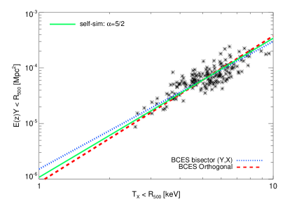
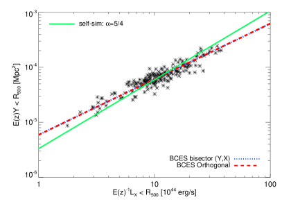
Figure 9: Relations between integrated Comptonization parameter and X-ray temperature and luminosity: $Y_{SZ}-T_{X}$ (left panel) and $Y_{SZ}-L_{X}$ (right panel). Best-fit lines for the Bisector and Orthogonal approaches are reported as in the legend. Self-similar curves are reported for comparison purposes (green, solid curves), normalized to the data at $5\rm{~{}keV}$ and $10^{45}\rm{~{}erg/s}$ for $T_{X}$ and $L_{X}$, respectively.

First, we investigate the relation between the integrated Comptonization parameter $Y_{SZ}$ (Eq. 12, with definition 13) and the X-ray temperature and “bolometric” luminosity ($T_{X}$ and $L_{X}$) within the projected $R_{500}$ (see, e.g., da Silva et al., 2004; Arnaud et al., 2007; Morandi et al., 2007; Melin et al., 2011).
The self-similar scaling of these quantities predicts:

$$E(z)\,Y_{SZ} \propto T^{5/2},$$ (14)

$$E(z)\,Y_{SZ} \propto (E(z)^{-1}L)^{5/4}.$$ (15)

In a more realistic picture, the additional complexity of baryonic processes is most-likely responsible for the deviation from the theoretical prediction. Additionally, observational limitations, such as instrumental response, projection effects and modelling of the data, also play a role in the final shape of reconstructed relations and in the discrepancy with theory.
Also in this case, we fit the synthetic data obtained for the MUSIC-2 clusters assuming a functional form similar to Eq. 5:

$${\rm Log}(E(z)\,Y_{SZ})={\rm Log}(C)+\alpha{\rm Log}({\rm X}),$$ (16)

where $Y_{SZ}$ is the SZ integrated Comptonization parameter given by Eq. 12 and re-definition as in Eq. 13, and the variable ${\rm X}$ is replaced either with $T_{X}$ (Eq. 14) or with $E(z)^{-1}L_{X}$ (Eq. 15). Both the integrated Comptonization parameter $Y_{SZ}$ and the normalization of the relations $C$ are given in units of $\rm{~{}Mpc}^{2}$, while the X-ray luminosity and temperature are in units of $10^{44}\rm{~{}erg/s}$ and $\rm{~{}keV}$, respectively.
For both these relations, it is not clear which variable between the two quantities involved should be treated as (in)dependent and a simple OLS minimization of the residuals in the Y variable would be most likely inappropriate to provide a reliable fit for the slope. Therefore, in order to correctly approach the problem, we employ also in this case the Bisector and Orthogonal methods and minimize the residuals of both variables with respect to the best-fit relation, providing results for both.
We show the scaling relations in Fig. 9 and report the best-fit values for slope and normalization, together with their 1-$\sigma$ errors, in Table 3. There we also list the scatter (Eq. 6) around the best-fit laws ($\sigma_{{\rm Log}Y}\sim 0.15$ for the $Y_{SZ}-T_{X}$ relation and $\sim 0.10$ for the $Y_{SZ}-L_{X}$).
From the values listed in Table 3 for the $Y_{SZ}-T_{X}$ relation we notice that the Orthogonal BCES method converges on steeper slopes than the Bisector method, as in the case of the $L_{X}-T_{X}$ scaling law. In particular, we find that the slope of the $Y_{SZ}-T_{X}$ relation better agrees with the predicted self-similar value than the slope of the $Y_{SZ}-L_{X}$ one, which is equally under-estimated by both Bisector and Orthogonal methods, rather suggesting a slope shallower than the self-similar prediction. Given that $Y_{SZ}$ closely traces the system mass, the deviation of $Y_{SZ}-L_{X}$ from self-similarity can be mainly related to the X-ray luminosity, which is more sensitive to the gas physics and dynamical state than to the temperature, as already shown in previous sections.
Comparing the correlations in Fig. 9, we note that these results are consistent with the departure of the $L_{X}-T_{X}$ scaling law from the self-similar trend previously discussed, which was steeper than theoretically predicted.
Additionally, this behaviour is fairly consistent with other results in the literature, e.g. with findings by da Silva et al. (2004) obtained from numerical simulations as well as with observational studies by Arnaud et al. (2007); Morandi et al. (2007); Melin et al. (2011); Planck Collaboration et al. (2011).

4.2.7 The $Y_{SZ}-Y_{X}$ relation

The cluster integrated thermal energy is quantified both by $Y_{SZ}$ and $Y_{X}$, with the main difference that the former depends on the mass-weighted temperature of the gas, while the latter is rather dependent on the X-ray temperature, resulting more sensitive to the lower-entropy gas. These two integrated quantities are therefore expected to correlate tightly, and the comparison allows us to test the thermal state of the ICM and the differences between the true and the X-ray temperature (see, e.g., Arnaud et al., 2010; Andersson et al., 2011; Fabjan et al., 2011; Kay et al., 2012).
In order to compare directly $Y_{SZ}$ and $Y_{X}$, we rescale the latter by the factor

$$C_{SZX}=\frac{\sigma_{T}}{m_{e}c^{2}}\frac{1}{\mu_{e}m_{p}}=1.43\times 10^{-19}\frac{\rm{~{}Mpc}^{2}}{\rm{~{}M_{\odot}}\rm{~{}keV}}$$ (17)

for a mean molecular weight of electrons $\mu_{e}=1.14$.
In Fig. 10 we show the $Y_{SZ}-Y_{X}$ relation, for the sample of 179 MUSIC clusters with $Y_{X}=M^{sim}_{g,500}T_{X}$ (Eq. 8). By using the true gas mass within $R_{500}$, calculated directly from the simulations, we explicitly investigate the role of temperature.
Indeed, since in this case no deviation is included because of the X-ray estimation of the total gas mass, the difference between the 1:1 relation and the best-fit line is substantially attributed to the mis-estimation of $T_{mw}$ by $T_{X}$. More evidently, the ratio $Y_{SZ}/C_{SZX}Y_{X}$ can be quantified by the best-fitting normalization of the relation when the slope is fixed to one.

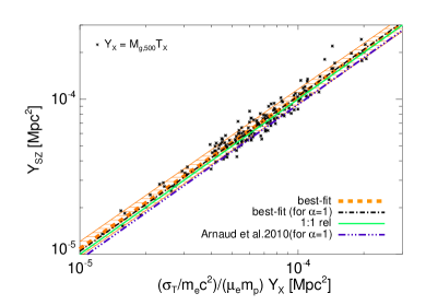
Figure 10: Relation between integrated Comptonization parameter $Y_{SZ}$ and the X-ray-analog quantity $Y_{X}=M_{g,500}T_{X}$. We display in the plot the best-fit relation to the data (orange, dashed line) and the one obtained by fixing the slope to 1 and fitting for the normalization only (black, dot-dashed), the 1:1 (self-similar) relation (green, solid line) and the observational result by Arnaud et al. (2010) (dot-dot-dot-dashed, purple line). The shaded orange area marks the $5\%$ scatter about the best-fit line.

An ideal measurement of the true temperature of the clusters would basically permit to evaluate by $Y_{X}$ the very same property of the ICM as done via $Y_{SZ}$, expecting an actual 1:1 correlation. Dealing with simulated galaxy clusters, this can be tested by employing the true $T_{mw}$ in Eq. 8. By applying this to our subsample of MUSIC clusters, we confirm this with very good precision.
When the spectroscopic temperature is instead employed, for a slope fixed to one in the best-fit, we observe a higher normalization, $C=1.05$ (for $Y_{SZ}$ and $Y_{X}$ both normalized to $5\times 10^{-4}\rm{~{}Mpc}^{2}$), with a scatter of roughly $5$ per cent. The deviation from one, $\sim 5\%$, is consistent with the mean deviation between mass-weighted and X-ray temperatures (see Fig. 3 and discussion in Section 4.1.2). Nevertheless, this deviation is also comparable to the scatter in the relation as, in fact, the $T_{mw}$ and $T_{X}$ estimates for this MUSIC sub-sample are in very good agreement.
Moreover, we note that the employment of the X-ray temperature generates a larger scatter about the relation, although relatively low with respect to previous (X-ray) relations ($\sigma_{{\rm Log}Y_{SZ}}\sim 0.05$). This confirms the robustness of $Y_{X}$ as a mass indicator, despite the minor deviations due to $T_{X}$. As a comparison, the ideal, reference test for $Y_{X}=M_{g,500}T_{mw}$ provides a remarkably tighter correlation, with a scatter smaller than one percent.
We also perform the linear fit to the $Y_{SZ}-C_{SZX}Y_{X}$ in the Log-Log plane in order to find the values of the slope and normalization that minimize the residuals, listed in Table 3 with the scatter in ${\rm Log}Y_{SZ}$. Even in this case, both slope and normalization are very close to the expected (self-similar) value of one, with a scatter of $\sim 5\%$.
As marked in Fig. 10 by the orange, dashed curve and shaded area around it (which indicates the $5\%$ scatter), the best-fit relation for MUSIC clusters is still consistent with the expected one-to-one relation.

Table 1: Best-fit parameters of the $L_{X}-T_{X}$ scaling relation: slope, normalization and scatter. The relation is normalized at the value of $T_{0}=5\rm{~{}keV}$. For comparison, we also report the expected self-similar slope.

		${\bf\alpha_{\rm self-sim}}$	${\bf\alpha}$	${\bf C}~{}[10^{44}\rm{~{}erg/s}]$	${\bf\sigma_{{\rm Log}Y_{SZ}}}$
${}^{\star}{L_{X}-T_{X}}$	BCES Bisector (Y,X)	$2$	$2.29\pm 0.07$	$10.03\pm 0.19$	$0.11$
	BCES Orthogonal	$2$	$2.46\pm 0.09$	$9.98\pm 0.19$	$0.11$

^⋆The luminosity considered is calculated over the maximum energy band defined by the Chandra ACIS-S response, as in Fig. 8.

Table 2: Best-fit parameters of the $Y_{SZ}-T_{X}$ and $Y_{SZ}-L_{X}$ scaling relations: slope, normalization and scatter. For comparison, we also report the expected self-similar slope.

		${\bf\alpha_{\rm self-sim}}$	${\bf\alpha}$	${\bf C}~{}[10^{-6}\rm{~{}Mpc}^{2}]$	${\bf\sigma_{{\rm Log}Y_{SZ}}}$
${Y_{SZ}-T_{X}}^{\star}$	BCES Bisector (Y,X)	$2.5$	$2.29\pm 0.09$	$1.52\pm 0.22$	$0.14$
	BCES Orthogonal	$2.5$	$2.64\pm 0.12$	$0.87\pm 0.17$	$0.16$
${Y_{SZ}-L_{X}}^{\star}$	BCES Bisector (Y,X)	$1.25$	$1.01\pm 0.03$	$5.95\pm 0.40$	$0.10$
	BCES Orthogonal	$1.25$	$1.01\pm 0.03$	$5.93\pm 0.43$	$0.10$

^⋆The luminosity and temperature considered are those employed in the $L_{X}-T_{X}$ relation (see Section 4.2.4).

Table 3: Best-fit parameters of the $Y_{SZ}-C_{SZX}Y_{X}$ scaling relation: slope, normalization and scatter, with different minimization methods. For comparison, we also report the expected self-similar slope.

		${\bf\alpha_{\rm self-sim}}$	${\bf\alpha}$	${\bf C^{{\dagger}}}$	${\bf\sigma_{{\rm Log}Y_{SZ}}}$
$Y_{SZ}-C_{SZX}Y_{X}$	OLS (Y,X)	1	$0.98\pm 0.01$	$1.01\pm 0.03$	0.05
	BCES Bisector (Y,X)	1	$1.00\pm 0.01$	$1.05\pm 0.03$	0.05
	BCES Orthogonal	1	$1.00\pm 0.01$	$1.05\pm 0.03$	0.05

^†Both $Y_{SZ}$ and $C_{SZX}Y_{X}$ are normalized at the pivot point $5\times 10^{-4}\rm{~{}Mpc}^{2}$, so that for the slope fixed to one, the normalization expresses directly the ratio $Y_{SZ}/C_{SZX}Y_{X}$.

4.2.8 Comparison to observational results

Despite the observational-like approach applied to derive X-ray properties, the MUSIC scaling relations still present some differences with respect to observational findings. The aim of this section is to discuss our results, and the level of agreement with previous observational and numerical studies, given the strong sensitivity of X-ray cluster properties to the modeling of the baryonic physics. To this end, we focus on the mass-temperature and luminosity-temperature relations, in order to close the circle between X-ray observables and intrinsic total mass.

$\mathbf{\bullet\,\,\,M_{500}-T_{X}.}$ In the calibration of the mass-temperature relation, the estimate of $T_{X}$ plays a role on the normalization as well. In order to investigate this aspect, we show in Fig. 11 the inverse relation $M_{500}-T_{X}$, as more commonly presented by several authors. The best-fit curve to the MUSIC data is again fitted, minimizing the residuals in ${\rm Log}T_{X}$ (OLS(X$|$Y)), as we consider here the true mass of the systems. Consistently with the findings for the $T_{X}-M_{500}$ scaling relation (Section 4.2.1), the slope here is steeper than self-similar. Moreover, compared to observational data, in particular to the relation by Arnaud et al. (2005), we find a higher normalization for the MUSIC sample. Part of this difference can be explained by the observational procedure to derive the total mass from the X-rays, which is known to under-estimate the true dynamical mass of the system (see early studies by Evrard 1990; Evrard et al. 1996 and more recent works by Rasia et al. 2006; Nagai et al. 2007; Piffaretti & Valdarnini 2008; Jeltema et al. 2008; Lau et al. 2009; Morandi et al. 2010; Rasia et al. 2012; Lau et al. 2013), i.e. the intrinsic value which is instead used for the MUSIC clusters. Nevertheless, additional effects must play a role in increasing the discrepancy, as this still persists when compared to other numerical works. Namely, the treatment of the baryonic physics in the MUSIC simulations can further contribute to this observed off-set, so that, for a fixed mass, the MUSIC clusters appear to be colder. This can be explored, as in Fig. 11, by comparing the MUSIC relation to simulation studies by Borgani et al. (2004) and Fabjan et al. (2011), that also involve the true mass of the systems. In particular, we focus on the sub-sample of MUSIC regular clusters, for which we find on average a very small bias between $T_{X}$ and $T_{mw}$. As a consistency check, we compare first against the results by Borgani et al. (2004) and Fabjan et al. (2011) (“CSF”), as they consider the same physical description of the gas as the MUSIC re-simulations, basically including cooling and star formation according to the standard model by Springel & Hernquist (2003). The difference with respect to the former is simply due to the difference in the temperature definition, which is the emission-weighted value in their case; with respect to Fabjan et al. (2011) (“CSF”), where $T_{mw}$ is used instead, we find indeed agreement between the two relations, within the scatter. When the MUSIC data are instead compared to the results by Fabjan et al. (2011) for runs including metal cooling and AGN feedback (“CSF-M-AGN”), we find a larger, although not prominent, deviation. As the mass considered is always the total intrinsic value from the simulation and $T_{X}$ in MUSIC clusters is close to the $T_{mw}$ estimate, we expect the discrepancy to be mainly due to the different models included to describe the baryonic processes.

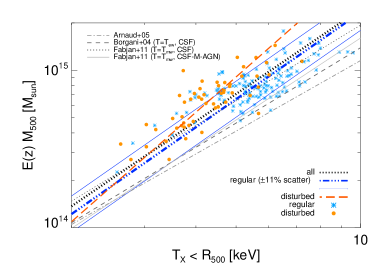
Figure 11: Total mass within $R_{500}$ as a function of temperature. Results are shown considering the X-ray spectroscopic temperature ($T_{X}$), for the regular (cyan asterisks) and disturbed (orange circles) sub-samples. Data and best-fit relations from observations by Arnaud et al. (2005) and from numerical studies by Borgani et al. (2004) and Fabjan et al. (2011) are also shown for comparison.

$\mathbf{\bullet\,\,\,\L_{X}-T_{X}.}$ Dealing with X-ray properties, the other fundamental quantity taken into account is the luminosity and its relationship with temperature. While the steepening of the MUSIC $L_{X}-T_{X}$ relation seems consistent, albeit weaker, with observational results, the normalization is higher than observed. In this case, even though some differences between the approach adopted with PHOX and other observational procedures exist, the limitations due to the treatment of the baryonic physics are likely to play a more significant role.
In fact, the lack of an efficient way to remove the hot-phase gas basically increases the amount of X-ray emitting ICM. This would be mitigated by the inclusion of AGN feedback, although the stronger effects are expected to be particularly important at group scales, while massive clusters like those in our sample ($T_{X}>2\rm{~{}keV}$) are generally less dramatically affected (as shown by both Puchwein et al. (2008) and Fabjan et al. (2010), despite the different implementations used). In Fig. 12 we show the luminosity-temperature relation for the two sub-samples of regular and disturbed clusters. For comparison we also report observational data by Pratt et al. (2009); Maughan et al. (2012) and results from numerical studies by Borgani et al. (2004); Jeltema et al. (2008); Puchwein et al. (2008); Fabjan et al. (2010); Biffi et al. (2013a). In order to minimize the effects due to X-ray temperature bias, we specifically focus on regular MUSIC clusters (for which $\alpha=2.53\pm 0.11$ and $C=9.32\pm 0.2110^{44}\rm{~{}erg/s}$).
Comparing, we note from Fig. 12 that for a given temperature the MUSIC clusters appear to be generally more luminous. On average, observations (as Pratt et al., 2009; Maughan et al., 2012) predict a luminosity of roughly $6-7\times 10^{44}\rm{~{}erg/s}$, at $T_{0}=5\rm{~{}keV}$, while we find a normalization higher by a factor of $\sim 20-30\%$. In fact, the inefficient feedback in the center can cause higher $L_{X}$. With respect to those observational works, the difference can be due in part also to the choice of not removing the core from the current analysis, where the over-cooling can affect the cluster central region.

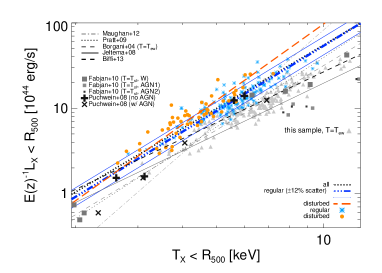
Figure 12: $L_{X}-T_{X}$ relation. The results for our sample are presented for both the regular and disturbed sub-sample of clusters (cyan asterisks and orange filled circles, respectively). Values corresponding to the emission-weighted temperature ($T_{ew}$, light-grey filled triangles) are also shown for comparison, as well as observational data by Maughan et al. (2012) and Pratt et al. (2009) and numerical findings by Borgani et al. (2004), Puchwein et al. (2008), Jeltema et al. (2008), Fabjan et al. (2010) and Biffi et al. (2013a).

With respect to simulation works employing a spectroscopic temperature, as in the numerical studies by Jeltema et al. (2008), Puchwein et al. (2008) (run with AGN feedback) and Biffi et al. (2013a), or a spectroscopic-like estimate, as in Fabjan et al. (2010) (where the authors use instead $T_{sl}$), the different normalization of the MUSIC relation must be mainly related to the missing treatment of AGN feedback or proper metal cooling. In fact, our findings are obviously consistent with simulations accounting for similar models of the baryonic processes (as for the run withough AGN feedback by Puchwein et al., 2008). This actually explains the diverse level of agreement between the MUSIC clusters and the results by Puchwein et al. (2008) (“w/ AGN” run) and Fabjan et al. (2010) (“AGN1” and “AGN2” runs), despite they both account for AGN feedback mechanisms.
Instead, the divergence from the best-fit relation by Borgani et al. (2004) might have a different origin. Notwithstanding the very similar modeling of the gas physics, the authors adopt there a different definition of the ICM temperature, namely the emission-weighted estimate, which brings the simulated relation closer to both observed results and more complete sets of hydrodynamical simulations (see Jeltema et al., 2008; Fabjan et al., 2010; Biffi et al., 2013a), predicting a luminosity of $\sim 5.6\times 10^{44}\rm{~{}erg/s}$ for $T_{0}=5\rm{~{}keV}$. As also confirmed by our analysis, in fact, $T_{ew}$ has been found (e.g. Mazzotta et al., 2004) to over-estimate the spectroscopic temperature, which is the one adopted here instead. Similarly, the use of $T_{ew}$ instead of $T_{X}$ for the MUSIC clusters would also provide a lower normalization ($C=5.87\pm 0.1510^{44}\rm{~{}erg/s}$) and a better agreement (see light-grey symbols in Fig. 12).
Additionally, we remark that also numerical resolution can affect the resulting $L_{X}$, which can be under-estimated in less resolved clusters. Instead, the results tend to reach stability for increasing resolution (see, for instance, Valdarnini, 2002). Hence, given the similar physical models treated, the lower normalization of the clusters in Borgani et al. (2004) can also be partially caused by their lower resolution with respect to the MUSIC re-simulations.

The two relations shown in Fig. 11 and Fig. 12 also provide the case to discuss the behaviour of the regular and disturbed cluster sub-samples. The two groups of objects clearly occupy different regions of the relations, having regular clusters on average higher temperatures. Calculating the two best-fit curves for the two sub-samples separately, we generally find that disturbed clusters provide steeper relations ($\alpha_{M-T}=\pm$ and $\alpha_{L-T}=2.96\pm 0.21$) with respect to regular objects ($\alpha_{M-T}=\pm$ and $\alpha_{L-T}=2.53\pm 0.11$). Moreover, the disagreement with previous observational and simulations studies is less significant for the regular sub-set of MUSIC clusters.
The very high statistics of our analysis also provides the case for studying and constraining the scatter of the relations with very good precision, despite the level of agreement in terms of slope and normalization. In fact, the scatter of the $L_{X}-T_{X}$, in particular, is usually significantly larger in real data (up to $50-70$ per cent, as in Pratt et al., 2009; Maughan et al., 2012) than for the MUSIC clusters, where instead $\sigma_{{\rm Log}L_{X}}\sim 0.11$. Considering the two sub-sets separately, the scatter about the best-fit relation is slightly different, indicating a tighter correlation in the first case and a more dispersed relation in the other, with $\sigma_{{\rm Log}L_{X}}\sim 0.10$ (marked by the two solid blue lines in Fig. 12) and $\sigma_{{\rm Log}L_{X}}\sim 0.12$, respectively. Similarly, while the scatter of the $M_{500}-T_{X}$ relation is $\sigma_{{\rm Log}M}\sim 0.10$ for the whole sample, the dispersion in ${\rm Log}M$ is found to be smaller for regular objects ($\sigma_{{\rm Log}M}\sim 0.09$, marked by the two solid blue lines in Fig. 11) and larger for the disturbed ones ($\sigma_{{\rm Log}M}\sim 0.11$).

5 Conclusions

This analysis presents results on the largest sample of high-resolution, simulated galaxy clusters ever analysed with observational approach by means of X-ray synthetic observations.
Thanks to the large MUSIC-2 data-set, we could obtain a complete volume-limited sample of re-simulated cluster-like objects. Out of these, we select a sub-sample of 179 massive haloes at $z=0.11$, comprising those matching the mass completeness ($M_{vir}>7.5\times 10^{14}h^{-1}\rm{~{}M_{\odot}}$) at the considered redshift ($z=0.11$), but also extending to all the progenitors of the systems with $M_{vir}>8.5\times 10^{14}h^{-1}\rm{~{}M_{\odot}}$ at $z=0$. Although restricted to a smaller sub-set, our principal goal with this work is to extend the analysis on the MUSIC-2 clusters Sembolini et al. (2013) by addressing their X-ray observable properties and scaling relations.
For all the selected objects, we generated ideal X-ray photon emission (by means of the code PHOX, Biffi et al., 2012) on the base of the gas thermal properties provided by the original hydrodynamical simulation. From regions up to $R_{500}$ centered on each cluster we then obtained Chandra synthetic observations that provided us with global X-ray properties, such as temperature and luminosity (Section 3).
First, we investigated the bias between the spectroscopic temperature measured from the synthetic spectra ($T_{X}$) and the theoretical estimates calculated directly from the simulation.
For the MUSIC sub-sample analysed, $T_{X}$ is on average lower then the true, mass-weighted value $T_{mw}$. While this is fairly consistent with studies by Mathiesen & Evrard (2001) and Kay et al. (2008); Kay et al. (2012), we observe some tension with X-ray mock studies of simulated clusters by, e.g., Nagai et al. (2007) and Piffaretti & Valdarnini (2008). This discrepancy can be ascribed to the multi-phase thermal structure of the ICM, whose temperature distribution plays an important role in the determination of the global temperature (see also the detailed discussion in Mazzotta et al., 2004). Indeed, a two-component model would improve the description of the multi-temperature structure and provide a better spectral fit, albeit with a resulting, evident over-estimation of the true temperature by the hotter component of the two. For the generally massive systems considered, this would generate a consequent non-negligible bias. Therefore, we still considered results from the single-temperature, keeping in mind the tendency by $T_{X}$ to a mild, average under-estimation of $T_{mw}$. This difference is very low in our estimates (roughly $5$ per cent, despite some dispersion; see Fig. 3) and we confirm an overall good correlation between $T_{X}$, within the projected $R_{500}$, and $M_{500}$ (Fig. 5).
The bias between $T_{X}$ and $T_{mw}$ is also showing some dependence on the level of dynamical disturbance of the cluster, quantified by the displacement between the system center of mass and peak of density. Specifically, regular clusters show an average bias which is consistent with zero (basically dominating the result for the entire sample), while the disturbed sub-set presents a more prominent under-estimation of $T_{mw}$ by $T_{X}$.
The observational-like derivation of the ICM temperature is also useful to investigate possible bias in the correlation with intrinsic propertiesobtained directly from the simulation, as in the $T_{X}-M_{500}$ (Section 4.2.1) and $Y_{SZ}-T_{X}$ (Section 4.2.5) relations. The effect has also been studied via the $Y_{X}$, where the observational-like $T_{X}$ is combined with the true $M_{g,500}$ (Section 4.2.3).
We find that:

• $T_{X}-M_{500}$ shows a larger scatter when $T_{X}$ is employed rather than $T_{mw}$ and a shallower slope than expected from the self-similar scaling (see Fig. 5);

• $Y_{SZ}-T_{X}$ is consistent with findings in observational studies, and deviations from self-similarity are less significant than for $Y_{SZ}-L_{X}$ (Section 4.2.5);

• correlations between $Y_{X}$ and gas or total mass indicate a slope very close to the self-similar value (Fig. 7);

• the employment of X-ray temperature only affects scatter and normalization of $M_{g,500}-Y_{X}$ and $M_{500}-Y_{X}$.

Similar considerations can be drawn when the $Y_{SZ}-Y_{X}$ scaling law is explored (Section 4.2.7). Here the normalization is slightly higher than one, albeit compatible, and the slope is remarkably close to self-similarity (see Table 3). In this case, also the scatter matches the expectation to be very low ($\sigma_{{\rm Log}Y_{SZ}}\sim 0.05$), although larger than in the ideal case of $Y_{X}=M_{g,500}T_{mw}$ (where its is $\lesssim 1\%$).
Unlike $T_{X}$, the X-ray luminosity is intrinsically less accurate to trace mass as it is particularly susceptible to the non-gravitational processes governing the gas physics. In fact, $L_{X}$ is difficult to model in numerical simulations and, from observations, it is found to add an intrinsic scatter to scaling relations. Here, we confirm that $L_{X}$ tends to augment the deviation from self-similarity as well as the scatter in the scaling with other intrinsic properties (such as total mass, SZ integrated Compton parameter or $Y_{X}$) and with X-ray temperature.
The $L_{X}-T_{X}$ scaling relation for this MUSIC sub-sample extends the study to a larger set of simulated clusters with respect to what previously done with simulations, especially involving a proper generation and derivation of observable X-ray quantities Puchwein et al. (2008); Fabjan et al. (2010); Biffi et al. (2013a, b). This relation is relatively easy to construct for real clusters as well and generally represents a crucial break of self-similarity. In fact, the observed slope significantly deviates from the self-similar prediction – typically $\alpha\sim 2.5-3$ instead of $\alpha_{\rm self-sim}=2$ (e.g. White et al., 1997; Markevitch, 1998; Arnaud & Evrard, 1999; Ikebe et al., 2002; Ettori et al., 2004; Maughan, 2007; Morandi et al., 2007; Zhang et al., 2008; Pratt et al., 2009; Maughan et al., 2012). MUSIC clusters also show a steeper slope than expected, albeit shallower than in real observations (see Table 3), when the residuals are minimized for both variables. Despite the possible deviations in slope and normalization, the increased statistics of this sample allows us to precisely estimate the scatter of the relation, which is found to be only $\sim 10\%$ in ${\rm Log}L_{X}$.
From the relations explored, we conclude that the interpretation of observational data and comparison to theoretical predictions can certainly benefit from the observational-like approach. In fact, a more faithful comparison is possible even when no additional complications related to the analysis of real data (e.g. background subtraction or spacial changes of the effective area) are included. This is especially true for the slope of the relations, which deviates from self-similarity in a similar way as in observational data.
Differently, the amplitude of the scaling relations is more sensitive to the accuracy of the physical description adopted in hydrodynamical simulations to model the baryonic processes.
In fact, the normalization of MUSIC scaling laws shows more tension with observational findings. We discuss this and the comparison to other simulation works for the $M_{500}-T_{X}$ and $L_{X}-T_{X}$ relations, which represent the two main steps to go from X-ray ICM properties to total mass, via scaling relations. Especially in the $L_{X}-T_{X}$ case we find that the normalization for MUSIC clusters is higher than both observations and more complete simulations. Inefficient cooling and feedback mechanisms, in fact, interplay and compete to moderately increasing the X-ray emitting gas in the central part of MUSIC clusters, thereby augmenting the luminosity and, simultaneously, reducing the temperature.
Certainly, more robust mass indicators that are not strongly affected by non-gravitational processes, such as $Y_{X}$, can be safely employed Kravtsov et al. (2006); Nagai et al. (2007); Fabjan et al. (2011). In fact, the low scatter around the MUSIC $Y_{SZ}-Y_{X}$, $M_{g,500}-Y_{X}$ and $M_{500}-Y_{X}$ relations is preserved, even when we use our observational estimates of the X-ray temperature. Moreover, in the specific case of $Y_{SZ}-Y_{X}$, the MUSIC clusters are also fairly compatible with observations.
Nevertheless, we remark that, given the increasingly detailed observations available with current and up-coming X-ray instruments (e.g. ASTRO-H and ATHENA+), a more complete modeling of the baryonic physical processes in simulations is required. Unavoidably, this also needs to be combined with a proper observational-like approach to derive X-ray properties. In this way, it will be possible to eventually minimize the distance between numerical hydro-simulations and observations, and correctly interpret the complex, underlying ICM physics.

Appendix A Effects on the temperature estimate of the single-temperature spectral fit.

We present here the results of the spectral fitting procedure (see Section 3.1), in terms of the reduced chi-squared statistics, $\chi^{2}_{red}$.
In Fig. 14 we show the $\chi^{2}_{red}$ distribution (as well as the cumulative one) of the best-fitting single-temperature models for the cluster sample. Additionally, we also show the dependence of the $T_{X}/T_{sim}$ ratio (see Section 4.1.2) on the fit $\chi^{2}_{red}$.

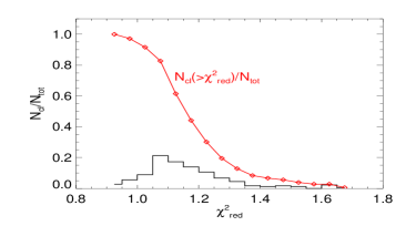
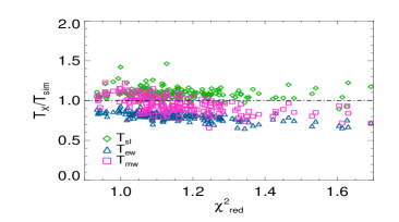
Figure 13: Distribution of the reduced-$\chi^{2}$ values of the best-fitting models for the clusters in the sample. Over-plotted is the cumulative distribution, $N_{cl}(>\chi^{2}_{red})/N_{tot}$ (solid, red line with diamonds).

Figure 14: Correlation of the temperature ratio $T_{X}/T_{sim}$ with the reduced $\chi^{2}$ obtained for the single-temperature fit of the cluster Chandra spectra. The ratio is reported for the three theoretical estimates of temperature: $T_{sl}$ (green), $T_{ew}$ (blue), $T_{mw}$ (pink). The region considered is always that enclosed by $R_{500}$ and the spectra are fitted over the entire $[0.5-10]\rm{~{}keV}$ band.

References

- Akritas & Bershady (1996) Akritas M. G., Bershady M. A., 1996, ApJ, 470, 706
- Allen et al. (2011) Allen S. W., Evrard A. E., Mantz A. B., 2011, ARA&A, 49, 409
- Andersson et al. (2011) Andersson K., Benson B. A., Ade P. A. R., Aird K. A., Armstrong B., Bautz M., Bleem L. E., Brodwin M., Carlstrom J. E., Chang C. L., Crawford T. M., Crites A. T., et al. 2011, ApJ, 738, 48
- Arnaud (1996) Arnaud K. A., 1996, in G. H. Jacoby & J. Barnes ed., Astronomical Data Analysis Software and Systems V Vol. 101 of Astronomical Society of the Pacific Conference Series, XSPEC: The First Ten Years. pp 17–+
- Arnaud & Evrard (1999) Arnaud M., Evrard A. E., 1999, MNRAS, 305, 631
- Arnaud et al. (2005) Arnaud M., Pointecouteau E., Pratt G. W., 2005, A&A, 441, 893
- Arnaud et al. (2007) Arnaud M., Pointecouteau E., Pratt G. W., 2007, A&A, 474, L37
- Arnaud et al. (2010) Arnaud M., Pratt G. W., Piffaretti R., Böhringer H., Croston J. H., Pointecouteau E., 2010, A&A, 517, A92
- Biffi et al. (2013a) Biffi V., Dolag K., Böhringer H., 2013a, MNRAS, 428, 1395
- Biffi et al. (2013b) Biffi V., Dolag K., Böhringer H., 2013b, Astronomische Nachrichten, 334, 317
- Biffi et al. (2012) Biffi V., Dolag K., Böhringer H., Lemson G., 2012, MNRAS, 420, 3545
- Bonamente et al. (2008) Bonamente M., Joy M., LaRoque S. J., Carlstrom J. E., Nagai D., Marrone D. P., 2008, ApJ, 675, 106
- Bonamente et al. (2006) Bonamente M., Joy M. K., LaRoque S. J., Carlstrom J. E., Reese E. D., Dawson K. S., 2006, ApJ, 647, 25
- Borgani & Kravtsov (2011) Borgani S., Kravtsov A., 2011, Advanced Science Letters, 4, 204
- Borgani et al. (2004) Borgani S., Murante G., Springel V., Diaferio A., Dolag K., Moscardini L., Tormen G., Tornatore L., Tozzi P., 2004, MNRAS, 348, 1078
- Comis et al. (2011) Comis B., De Petris M., Conte A., Lamagna L., De Gregori S., 2011, MNRAS, 418, 1089
- da Silva et al. (2004) da Silva A. C., Kay S. T., Liddle A. R., Thomas P. A., 2004, MNRAS, 348, 1401
- D’Onghia & Navarro (2007) D’Onghia E., Navarro J. F., 2007, MNRAS, 380, L58
- Eckmiller et al. (2011) Eckmiller H. J., Hudson D. S., Reiprich T. H., 2011, A&A, 535, A105
- Ettori et al. (2004) Ettori S., Borgani S., Moscardini L., Murante G., Tozzi P., Diaferio A., Dolag K., Springel V., Tormen G., Tornatore L., 2004, MNRAS, 354, 111
- Ettori et al. (2012) Ettori S., Rasia E., Fabjan D., Borgani S., Dolag K., 2012, MNRAS, 420, 2058
- Ettori et al. (2004) Ettori S., Tozzi P., Borgani S., Rosati P., 2004, A&A, 417, 13
- Evrard (1990) Evrard A. E., 1990, ApJ, 363, 349
- Evrard et al. (1996) Evrard A. E., Metzler C. A., Navarro J. F., 1996, ApJ, 469, 494
- Fabjan et al. (2011) Fabjan D., Borgani S., Rasia E., Bonafede A., Dolag K., Murante G., Tornatore L., 2011, MNRAS, 416, 801
- Fabjan et al. (2010) Fabjan D., Borgani S., Tornatore L., Saro A., Murante G., Dolag K., 2010, MNRAS, 401, 1670
- Gardini et al. (2004) Gardini A., Rasia E., Mazzotta P., Tormen G., De Grandi S., Moscardini L., 2004, MNRAS, 351, 505
- Giodini et al. (2013) Giodini S., Lovisari L., Pointecouteau E., Ettori S., Reiprich T. H., Hoekstra H., 2013, SSR, 177, 247
- Ikebe et al. (2002) Ikebe Y., Reiprich T. H., Böhringer H., Tanaka Y., Kitayama T., 2002, A&A, 383, 773
- Isobe et al. (1990) Isobe T., Feigelson E. D., Akritas M. G., Babu G. J., 1990, ApJ, 364, 104
- Jeltema et al. (2008) Jeltema T. E., Hallman E. J., Burns J. O., Motl P. M., 2008, ApJ, 681, 167
- Kaiser (1986) Kaiser N., 1986, MNRAS, 222, 323
- Kay et al. (2012) Kay S. T., Peel M. W., Short C. J., Thomas P. A., Young O. E., Battye R. A., Liddle A. R., Pearce F. R., 2012, MNRAS, 422, 1999
- Kay et al. (2008) Kay S. T., Powell L. C., Liddle A. R., Thomas P. A., 2008, MNRAS, 386, 2110
- Klypin et al. (2001) Klypin A., Kravtsov A. V., Bullock J. S., Primack J. R., 2001, ApJ, 554, 903
- Knebe & Power (2008) Knebe A., Power C., 2008, ApJ, 678, 621
- Komatsu et al. (2011) Komatsu E., Smith K. M., Dunkley J., Bennett C. L., Gold B., Hinshaw G., Jarosik e. a., 2011, ApJS, 192, 18
- Kravtsov & Borgani (2012) Kravtsov A. V., Borgani S., 2012, ARA&A, 50, 353
- Kravtsov et al. (1997) Kravtsov A. V., Klypin A. A., Khokhlov A. M., 1997, ApJS, 111, 73
- Kravtsov et al. (2006) Kravtsov A. V., Vikhlinin A., Nagai D., 2006, ApJ, 650, 128
- Lau et al. (2009) Lau E. T., Kravtsov A. V., Nagai D., 2009, ApJ, 705, 1129
- Lau et al. (2013) Lau E. T., Nagai D., Nelson K., 2013, ApJ, 777, 151
- Macciò et al. (2007) Macciò A. V., Dutton A. A., van den Bosch F. C., Moore B., Potter D., Stadel J., 2007, MNRAS, 378, 55
- Markevitch (1998) Markevitch M., 1998, ApJ, 504, 27
- Mathiesen & Evrard (2001) Mathiesen B. F., Evrard A. E., 2001, ApJ, 546, 100
- Maughan (2007) Maughan B. J., 2007, ApJ, 668, 772
- Maughan et al. (2012) Maughan B. J., Giles P. A., Randall S. W., Jones C., Forman W. R., 2012, MNRAS, 421, 1583
- Mazzotta et al. (2004) Mazzotta P., Rasia E., Moscardini L., Tormen G., 2004, MNRAS, 354, 10
- McCarthy et al. (2003) McCarthy I. G., Babul A., Holder G. P., Balogh M. L., 2003, ApJ, 591, 515
- Melin et al. (2011) Melin J.-B., Bartlett J. G., Delabrouille J., Arnaud M., Piffaretti R., Pratt G. W., 2011, A&A, 525, A139
- Meneghetti et al. (2010) Meneghetti M., Rasia E., Merten J., Bellagamba F., Ettori S., Mazzotta P., Dolag K., Marri S., 2010, A&A, 514, A93
- Morandi et al. (2007) Morandi A., Ettori S., Moscardini L., 2007, MNRAS, 379, 518
- Morandi et al. (2010) Morandi A., Pedersen K., Limousin M., 2010, ApJ, 713, 491
- Morrison & McCammon (1983) Morrison R., McCammon D., 1983, ApJ, 270, 119
- Nagai (2006) Nagai D., 2006, ApJ, 650, 538
- Nagai et al. (2007) Nagai D., Vikhlinin A., Kravtsov A. V., 2007, ApJ, 655, 98
- Neto et al. (2007) Neto A. F., Gao L., Bett P., Cole S., Navarro J. F., Frenk C. S., White S. D. M., Springel V., Jenkins A., 2007, MNRAS, 381, 1450
- Piffaretti & Valdarnini (2008) Piffaretti R., Valdarnini R., 2008, A&A, 491, 71
- Planck Collaboration (2013) Planck Collaboration 2013, A&A, 550, A129
- Planck Collaboration et al. (2011) Planck Collaboration Ade P. A. R., Aghanim N., Arnaud M., Ashdown M., Aumont J., Baccigalupi C., Balbi A., Banday A. J., Barreiro R. B., et al. 2011, A&A, 536, A11
- Prada et al. (2012) Prada F., Klypin A. A., Cuesta A. J., Betancort-Rijo J. E., Primack J., 2012, MNRAS, 423, 3018
- Pratt et al. (2009) Pratt G. W., Croston J. H., Arnaud M., Böhringer H., 2009, A&A, 498, 361
- Puchwein et al. (2008) Puchwein E., Sijacki D., Springel V., 2008, ApJ, 687, L53
- Rasia et al. (2006) Rasia E., Ettori S., Moscardini L., Mazzotta P., Borgani S., Dolag K., Tormen G., Cheng L. M., Diaferio A., 2006, MNRAS, 369, 2013
- Rasia et al. (2005) Rasia E., Mazzotta P., Borgani S., Moscardini L., Dolag K., Tormen G., Diaferio A., Murante G., 2005, ApJ, 618, L1
- Rasia et al. (2012) Rasia E., Meneghetti M., Martino R., Borgani S., Bonafede A., Dolag K., Ettori S., Fabjan D., Giocoli C., Mazzotta P., Merten J., Radovich M., Tornatore L., 2012, New Journal of Physics, 14, 055018
- Sarazin (1986) Sarazin C. L., 1986, Reviews of Modern Physics, 58, 1
- Sembolini et al. (2013) Sembolini F., De Petris M., Yepes G., Foschi E., Lamagna L., Gottlöber S., 2013, ArXiv e-prints
- Sembolini et al. (2013) Sembolini F., Yepes G., De Petris M., Gottlöber S., Lamagna L., Comis B., 2013, MNRAS, 429, 323
- Smith et al. (2001) Smith R. K., Brickhouse N. S., Liedahl D. A., Raymond J. C., 2001, ApJ, 556, L91
- Springel (2005) Springel V., 2005, MNRAS, 364, 1105
- Springel & Hernquist (2003) Springel V., Hernquist L., 2003, MNRAS, 339, 289
- Springel et al. (2001) Springel V., White M., Hernquist L., 2001, ApJ, 549, 681
- Sunyaev & Zeldovich (1970) Sunyaev R. A., Zeldovich Y. B., 1970, Ap&SS, 7, 3
- Sunyaev & Zeldovich (1972) Sunyaev R. A., Zeldovich Y. B., 1972, Comments on Astrophysics and Space Physics, 4, 173
- Suto et al. (2013) Suto D., Kawahara H., Kitayama T., Sasaki S., Suto Y., Cen R., 2013, ApJ, 767, 79
- Valdarnini (2002) Valdarnini R., 2002, ApJ, 567, 741
- Valdarnini (2006) Valdarnini R., 2006, New Astronomy, 12, 71
- Vazza et al. (2009) Vazza F., Brunetti G., Kritsuk A., Wagner R., Gheller C., Norman M., 2009, A&A, 504, 33
- White et al. (1997) White D. A., Jones C., Forman W., 1997, MNRAS, 292, 419
- Zhang et al. (2008) Zhang Y.-Y., Finoguenov A., Böhringer H., Kneib J.-P., Smith G. P., Kneissl R., Okabe N., Dahle H., 2008, A&A, 482, 451