Confirmation of bistable stellar differential rotation profiles

Abstract

Context. Solar-like differential rotation is characterized by a rapidly rotating equator and slower poles. However, theoretical models and numerical simulations can also result in a slower equator and faster poles when the overall rotation is slow.

Aims. We study the critical rotational influence under which differential rotation flips from solar-like (fast equator, slow poles) to an anti-solar one (slow equator, fast poles). We also estimate the non-diffusive ($\Lambda$ effect) and diffusive (turbulent viscosity) contributions to the Reynolds stress.

Methods. We present the results of three-dimensional numerical simulations of mildly turbulent convection in spherical wedge geometry. Here we apply a fully compressible setup which would suffer from a prohibitive time step constraint if the real solar luminosity was used. To avoid this problem while still representing the same rotational influence on the flow as in the Sun, we increase the luminosity by a factor of roughly $10^{6}$ and the rotation rate by a factor of $10^{2}$. We regulate the convective velocities by varying the amount of heat transported by thermal conduction, turbulent diffusion, and resolved convection.

Results. Increasing the efficiency of resolved convection leads to a reduction of the rotational influence on the flow and a sharp transition from solar-like to anti-solar differential rotation for Coriolis numbers around 1.3. We confirm the recent finding of a large-scale flow bistability: contrasted with running the models from an initial condition with unprescribed differential rotation, the initialization of the model with certain kind of rotation profile sustains the solution over a wider parameter range. The anti-solar profiles are found to be more stable against perturbations in the level of convective turbulent velocity than the solar-type solutions.

Conclusions. Our results may have implications for real stars that start their lives as rapid rotators implying solar-like rotation in the early main-sequence evolution. As they slow down, they might be able to retain solar-like rotation for lower Coriolis numbers, and thus longer in time, before switching to anti-solar rotation. This could partially explain the puzzling findings of anti-solar rotation profiles for models in the solar parameter regime.

1 Introduction

The solar surface differential rotation is characterized by a fast equator and a monotonic decrease of angular velocity toward the poles. The internal rotation of the Sun is such that only weak radial shear is present in the bulk of the convection zone. Strong shear is present only in the boundary layers at the bottom in the tachocline and in the near-surface shear layer (e.g. Thompson et al. 2003; Miesch & Toomre 2009, and references therein). The differential rotation is explained by the interaction of anisotropic turbulence and rotation, which is represented by a non-diffusive contribution to the Reynolds stress known as $\Lambda$ effect in mean-field hydrodynamics (Krause & Rüdiger 1974; Rüdiger 1980, 1989). Furthermore, turbulent latitudinal heat fluxes, or stably stratified layers below (Brun et al. 2011) or above (Warnecke et al. 2013) the convection zone are needed to explain why the Taylor–Proudman balance is broken in the Sun. Mean-field models with these ingredients or other parameterizations have been successful in reproducing the solar rotation profile (e.g. Brandenburg et al. 1992; Kitchatinov & Rüdiger 1995; Rempel 2005; Hotta & Yokoyama 2011), and recently also the tachocline and the near-surface shear layer (e.g. Kitchatinov & Olemskoy 2011).

Mean-field models rarely produce anti-solar differential rotation unless a strong meridional circulation is imposed (Kitchatinov & Rüdiger 2004). This suggestion is supported by simulations of Dobler et al. (2006), which displayed anti-solar differential rotation in their fully convective models as a consequence of strong meridional circulation. An arguably similar pathway was offered by Aurnou et al. (2007), who proposed that strong mixing by turbulent convection would be the primary agent for angular momentum equilibration and thus anti-solar differential rotation. This mixing must then be stronger in the meridional plane than in the azimuthal direction to produce negative differential rotation, similar to what is expected to occur in the near-surface shear layer of the Sun (Kitchatinov & Rüdiger 2005). Differential rotation and meridional circulation are intimately coupled (Kippenhahn 1963), and one implies the other. Anti-solar differential rotation implies a counter-clockwise circulation in the northern hemisphere, corresponding to poleward motion at the surface. In the context of the solar near-surface shear layer, this mechanism is referred to as gyroscopic pumping (Miesch & Hindman 2011).

Both mean-field models and simulations have limitations. Furthermore, approximations like first-order smoothing are used to derive turbulent transport coefficients, such as turbulent viscosity and the so-called $\Lambda$ effect. However, their range of validity in stellar convection zones is questionable and only limited comparisons between hydrodynamic mean-field models and direct simulations have been performed (see, however Rieutord et al. 1994). Direct numerical simulations of convection, on the other hand, lack small-scale structure and tend to be dominated by structures that span the entire convection zone.

The rotational influence on the flow can be measured by the local Coriolis number ${\rm Co}=2\Omega\tau$, where $\Omega$ is the rotation rate and $\tau$ is the turnover time. It is large in the bulk of the solar convection zone, especially if $\tau$ is estimated from mixing length theory, which predicts values of ${\rm Co}$ ranging from $10^{-3}$ near the surface to more than $10$ in the deep layers (e.g. Ossendrijver 2003; Brandenburg & Subramanian 2005; Käpylä 2011). This is not captured by present simulations, which might well be due to insufficient density stratification in most numerical simulations so far. Whether the deep layers of stellar convection zones are really like this remains an open question. Observational evidence also points to anti-solar differential rotation in some slowly rotating stars (e.g. Strassmeier et al. 2003; Weber et al. 2005) and solar-like rotation in rapidly rotating dwarfs (e.g. Collier Cameron 2002). However, for the star with the best observational evidence for anti-solar differential rotation, namely the single K giant star HD 31993 (Strassmeier et al. 2003), the Coriolis number is around unity and thus close to the expected transition.

Recent numerical studies have explored the transition from anti-solar to solar-like differential rotation (Brun & Palacios 2009; Chan 2010; Käpylä et al. 2011b, a; Gastine et al. 2013, 2014; Guerrero et al. 2013). Here we concentrate on the effect of superabiabaticity on the rotational influence and resulting large-scale flows, and study the bistability of the differential rotation first reported by Gastine et al. (2014) using Boussinesq convection. They found that, near the transition from anti-solar to solar-like differential rotation, both kinds of solutions are possible – depending on the initial conditions. This is interesting for stellar applications because most stars rotate rapidly when they are born and slow down due to magnetic braking. Rapid rotation implies solar-like differential rotation, which might then persist despite the angular momentum loss due to stellar winds.

In this paper we set out to study the transition of solar-like rotation profiles into the anti-solar regime, extending the work of Gastine et al. (2014) into models of compressible convection. Using the spherical wedge model employed in various previous papers, the essential parts summarized in Section 2, we investigate the effect of changing the rotational influence by modifying the radiative conductivity that has an effect on the convective velocities. We perform two types of simulations, presented in Section 3. Firstly, we run models from scratch, i.e. without an initially prescribed rotation profile, and locate the solar to anti-solar transition in terms of Coriolis number. Secondly, we investigate the dependence of the solutions on initial conditions by running models from solar and anti-solar states, with otherwise identical parameters.

2 The Model

Our hydrodynamic model is essentially the same as the one used in Käpylä et al. (2011a). The same model has also been used to model convection-driven dynamos (Käpylä et al. 2012, 2013; Cole et al. 2014). The computational domain is a wedge in spherical polar coordinates, where $(r,\theta,\phi)$ are radius, colatitude, and longitude. The radial, latitudinal, and longitudinal extents of the wedge are $r_{0}\leq r\leq r_{1}$, $\theta_{0}\leq\theta\leq\pi-\theta_{0}$, and $0\leq\phi\leq\phi_{0}$, respectively, where $r_{0}=0.72\,R_{\odot}$ and $r_{1}=0.97\,R_{\odot}$ denote the positions of the bottom and top of the computational domain, and $R_{\odot}=7\cdot 10^{8}$m is the radius of the Sun. Here we consider $\theta_{0}=\pi/12$ and $\phi_{0}=\pi/2$, so we cover a quarter of the azimuthal extent between $\pm 75^{\circ}$ latitude. The dependence on the latitudinal extent of the wedge was studied by Käpylä et al. (2011b), who found that the results are robust as long as the opening angle of the wedge is more than 90 degrees. We solve the compressible hydrodynamic equations,

$$\frac{D\ln\rho}{Dt}=-\bm{\nabla}\cdot\bm{u},$$ (1)

$$\frac{D\bm{u}}{Dt}=\bm{g}-2\bm{\Omega}_{0}\times\bm{u}+\frac{1}{\rho}\left(\bm{\nabla}\cdot 2\nu\rho\bm{\mathsf{S}}-\bm{\nabla}p\right),$$ (2)

$$T\frac{Ds}{Dt}=-\frac{1}{\rho}\bm{\nabla}\cdot\left({\bm{F}^{\rm rad}}+{\bm{F}^{\rm SGS}}\right)+2\nu\bm{\mathsf{S}}^{2},$$ (3)

where $D/Dt=\partial/\partial t+\bm{u}\cdot\bm{\nabla}$ is the advective time derivative, $\rho$ is the density, $\nu$ is the constant kinematic viscosity,

$${\bm{F}^{\rm rad}}=-K\bm{\nabla}T\quad\mbox{and}\quad{\bm{F}^{\rm SGS}}=-\chi_{\rm SGS}\rho T\bm{\nabla}s$$ (4)

are radiative and subgrid-scale (hereafter SGS) heat fluxes, where $K$ is the radiative heat conductivity and $\chi_{\rm SGS}$ is the turbulent heat conductivity, which represents the unresolved convective transport of heat (Käpylä et al. 2013) and was referred to as $\chi_{\rm t}$ in Käpylä et al. (2011a, 2012). Furthermore, $s$ is the specific entropy, $T$ is the temperature, and $p$ is the pressure. The fluid obeys the ideal gas law with $p=(\gamma-1)\rho e$, where $\gamma=c_{\rm P}/c_{\rm V}=5/3$ is the ratio of specific heats at constant pressure and volume, respectively, and $e=c_{\rm V}T$ is the specific internal energy. The rate of strain tensor $\bm{\mathsf{S}}$ is given by

$$\mathsf{S}_{ij}={\textstyle{1\over 2}}(u_{i;j}+u_{j;i})-{\textstyle{1\over 3}}\delta_{ij}\bm{\nabla}\cdot\bm{u},$$ (5)

where the semicolons denote covariant differentiation (Mitra et al. 2009).

The gravitational acceleration is given by $\bm{g}=-GM_{\odot}\bm{r}/r^{3}$, where $G=6.67\cdot 10^{-11}$ m³ kg^-1 s^-2 is the gravitational constant, and $M_{\odot}=2.0\cdot 10^{30}$ kg is the mass of the Sun. We neglect self-gravity of the matter in the convection zone. Furthermore, the rotation vector $\bm{\Omega}_{0}$ is given by $\bm{\Omega}_{0}=(\cos\theta,-\sin\theta,0)\Omega_{0}$.

2.1 Initial and boundary conditions

Here we make an effort to connect the model more closely with the parameters of the Sun. Due to the fully compressible formulation of our model, we are faced with a prohibitive time step limitation if we were to use the solar luminosity. As explained in detail in Käpylä et al. (2013), we circumvent this by using a roughly $10^{6}$ times higher luminosity in the model in comparison to the Sun. As the convective energy flux scales as $F_{\rm conv}\sim\rho u^{3}$, the convective velocity $u$ is roughly 100 times greater in the simulations than in the Sun. To obtain the same rotational influence on the flow as in the Sun, we must therefore increase $\Omega$ by the same factor. In general, this can be written as

$${\bm{u}}_{\rm sim}=L_{\rm ratio}^{1/3}{\bm{u}}_{\odot}\quad{\rm and}\quad\Omega_{\rm sim}=L_{\rm ratio}^{1/3}\Omega_{\odot},$$ (6)

where $L_{\rm ratio}=L_{0}/L_{\odot}$, with $L_{0}$ and $L_{\odot}\approx 3.84\cdot 10^{26}$ W being the luminosities of the model and the Sun, respectively, and $\Omega_{\odot}\approx 2.7\cdot 10^{-6}$s^-1 is the mean solar rotation rate, corresponding to $430$ nHz. In what follows we scale our results back to solar units so that, say for the velocity, we quote ${\bm{u}}_{\rm sim}/L_{\rm ratio}^{1/3}$. The scaling used here is based on dimensional arguments. It is supported by mixing length theory (Vitense 1953) and simulations (Brandenburg et al. 2005; Miesch et al. 2012), and should be applicable as long as the energy transport is not yet affected by rotation (see e.g. Yadav et al. 2013). Furthermore, we assume that the density and the temperature at the base of the convection zone at $r=0.72R_{\odot}$ have the solar values $\rho_{0}=200$ kg m^-3 and $T_{0}=2.23\cdot 10^{6}$K.

The initial state is isentropic and the hydrostatic temperature gradient is given by

$$\frac{\partial T}{\partial r}=-\frac{GM_{\odot}/r^{2}}{c_{\rm V}(\gamma-1)(n_{\rm ad}+1)},$$ (7)

where $n_{\rm ad}=1.5$ is the polytropic index for an adiabatic stratification. We fix the value of $\partial T/\partial r$ on the lower boundary. The density profile follows from hydrostatic equilibrium. To speed up the thermal relaxation, the initial condition is chosen not to be in thermodynamic equilibrium, but closer to the final convecting state. We choose the heat conduction profile such that radiative diffusion is responsible for supplying the energy flux in the system and progressively less so further out by choosing a radiative conductivity, $K(r)=K_{0}[n(r)+1]$, with $n(r)=\delta n(r/r_{0})^{-15}+n_{\rm ad}-\delta n$ replacing the polytropic index,

$$K_{0}=(\mathcal{L}/4\pi)c_{\rm V}(\gamma-1)(n_{\rm ad}+1)\rho_{0}\sqrt{GMR},$$ (8)

being a reference conductivity, and $\mathcal{L}$ being the non-dimensional luminosity, given below. Now $n=n_{\rm ad}$ at the bottom of the convection zone and approaches $n_{\rm ad}-\delta n$ at the surface. This means that $K=(n+1)K_{0}$ decreases toward the surface like $r^{-15}$ such that the value of $\delta n$ regulates the flux that is carried by convection (Brandenburg et al. 2005). Initial, final, and hydrostatic profiles of the temperature and density as well as the profiles of ${\rm Pr}_{\rm SGS}=\nu/\chi_{\rm SGS}$ and ${\rm Pr}=\nu/\chi$, where $\chi=K/\rho c_{\rm P}$, are shown in Fig. 1. We introduce weak small-scale Gaussian noise velocity perturbations in the initial state.

Our simulations are defined by the energy flux imposed at the bottom boundary, $F_{\rm b}=-(K\partial T/\partial r)|_{r=r_{0}}$ as well as the values of $\Omega_{0}$, $\nu$, and $\overline{\chi}_{\rm SGS}=\chi_{\rm SGS}(r_{\rm m}=0.845\,R_{\odot})$. Furthermore, the radial profile of $\chi_{\rm SGS}$ is piecewise constant above $r>0.75R_{\odot}$ with $\chi_{\rm SGS}=\overline{\chi}_{\rm SGS}$ at $0.75R_{\odot}<r<0.95R_{\odot}$, and $\chi_{\rm SGS}=1.35\overline{\chi}_{\rm SGS}$ above $r=0.95R_{\odot}$. Below $r=0.75R_{\odot}$, $\chi_{\rm SGS}$ tends smoothly to zero; see Fig. 1 of Käpylä et al. (2011a). We fix the value of $\chi_{\rm SGS}$ such that it corresponds to $5\cdot 10^{8}\,{\rm m}^{2}\,{\rm s}^{-1}$ in physical units at $r=r_{1}$.

The radial and latitudinal boundaries are assumed to be impenetrable and stress free, i.e.,

$$\!\!\!u_{r}=0,\quad\frac{\partial u_{\theta}}{\partial r}=\frac{u_{\theta}}{r},\quad\frac{\partial u_{\phi}}{\partial r}=\frac{u_{\phi}}{r}\quad(r=r_{0},r_{1}),$$ (9)

$$\!\!\!\frac{\partial u_{r}}{\partial\theta}=u_{\theta}=0,\quad\frac{\partial u_{\phi}}{\partial\theta}=u_{\phi}\cot\theta\quad(\theta=\theta_{0},\pi-\theta_{0}).\quad$$ (10)

Density and specific entropy have vanishing first derivatives on the latitudinal boundaries, thus suppressing heat fluxes through them.

On the outer radial boundary we apply a black body condition

$$\sigma T^{4}=-K\nabla_{r}T-\chi_{\rm SGS}\rho T\nabla_{r}s,$$ (11)

where $\sigma$ is the Stefan–Boltzmann constant. We use a modified value for $\sigma$ that takes into account that both surface temperature and energy flux through the domain are larger than in the Sun. We choose $\sigma$ such that the flux at the surface, $\sigma T^{4}$, carries the total luminosity through the boundary in the initial non-convecting state.

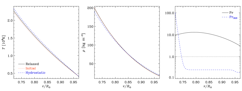
Figure 1: Left and middle panels: temperature $T$ in units of $10^{6}\,{\rm K}$ and density $\rho$ in units of $\,{\rm kg}\,{\rm m}^{-3}$, respectively, for the thermally relaxed state (black solid line), initial condition (red dotted), and hydrostatic solutions (blue dashed). Rightmost panel: Prandtl numbers related to radiative diffusion ${\rm Pr}=\nu/\chi$ where $\chi=K/\rho c_{\rm P}$ (black solid line), and the turbulent heat conductivity ${\rm Pr}_{\rm SGS}=\nu/\chi_{\rm SGS}$ (blue dashed) as functions of radius. Data is taken from Run D.

Table 1: Summary of the runs.

$$\begin{array}[]{p{0.05\linewidth}ccccccrrcccccccc}\hline\cr\vskip 3.0pt plus 1.0pt minus 1.0pt\cr Run&{\rm Ra}&{\rm Pr}&\delta n&{\rm Ro}_{\rm c}&{\rm Re}&{\rm Co}&\Delta_{\Omega}^{(\theta)}&\Delta_{\Omega}^{(r)}&\tilde{E}_{\rm kin}[10^{-7}]&E_{\rm mer}/E_{\rm kin}&E_{\rm rot}/E_{\rm kin}&\tilde{L}_{\rm rad}&\tilde{L}_{\rm conv}&{\rm remarks}\\ \hline\cr A&3.93\cdot 10^{5}&40.4&2.50&0.73&35&1.24&-2.47&-0.51&4.20&0.003&0.954&0.09&1.01&{\rm AS}\\ B&3.54\cdot 10^{5}&20.3&2.25&0.69&34&1.27&-2.36&-0.50&3.87&0.003&0.954&0.18&0.84&{\rm AS}\\ C&3.16\cdot 10^{5}&13.6&2.00&0.65&33&1.33&-2.28&-0.49&3.60&0.003&0.955&0.30&0.66&{\rm AS}\\ D&2.92\cdot 10^{5}&11.3&1.85&0.63&29&1.50&0.03&0.04&0.33&0.001&0.466&0.34&0.62&{\rm SL}\\ E&2.77\cdot 10^{5}&10.1&1.75&0.61&27&1.60&-0.01&0.09&0.38&0.001&0.593&0.37&0.53&\mbox{SL, polar jet}\\ \hline\cr D0&2.92\cdot 10^{5}&11.3&1.85&0.63&29&1.50&0.03&0.04&0.33&0.001&0.466&0.34&0.62&{\rm SL}\\ D1&3.16\cdot 10^{5}&13.5&2.00&0.65&29&1.50&0.16&0.07&0.37&0.001&0.517&0.28&0.65&{\rm SL}\\ D2&3.31\cdot 10^{5}&15.6&2.10&0.67&30&1.44&0.13&0.05&0.37&0.001&0.465&0.24&0.72&{\rm SL}\\ D3&3.47\cdot 10^{5}&18.4&2.20&0.68&32&1.37&0.03&0.01&0.28&0.002&0.243&0.21&0.81&{\rm SL}\\ D4&3.62\cdot 10^{5}&22.7&2.30&0.70&35&1.27&-2.33&-0.50&3.93&0.003&0.955&0.19&0.87&{\rm AS}\\ \hline\cr B0&3.54\cdot 10^{5}&20.3&2.25&0.69&34&1.27&-2.36&-0.50&3.87&0.003&0.954&0.18&0.84&{\rm AS}\\ B1&3.47\cdot 10^{5}&18.5&2.20&0.68&34&1.27&-2.26&-0.50&3.92&0.002&0.956&0.24&0.85&{\rm AS}\\ B2&3.31\cdot 10^{5}&15.7&2.10&0.67&33&1.31&-2.27&-0.50&3.87&0.003&0.958&0.27&0.77&{\rm AS}\\ B3&3.16\cdot 10^{5}&13.6&2.00&0.65&33&1.34&-2.18&-0.49&3.67&0.003&0.958&0.31&0.71&{\rm AS}\\ B4&3.00\cdot 10^{5}&12.0&1.90&0.64&32&1.37&-2.15&-0.49&3.54&0.003&0.958&0.34&0.64&{\rm AS}\\ B5&2.85\cdot 10^{5}&10.8&1.80&0.62&31&1.41&-2.06&-0.49&3.38&0.003&0.958&0.38&0.59&{\rm AS}\\ B6&2.69\cdot 10^{5}&9.7&1.70&0.60&30&1.45&-1.98&-0.48&3.16&0.003&0.957&0.41&0.54&{\rm AS}\\ B7&2.38\cdot 10^{5}&8.2&1.50&0.57&28&1.54&-1.86&-0.47&2.83&0.003&0.958&0.48&0.44&{\rm AS}\\ B8&2.22\cdot 10^{5}&7.6&1.40&0.55&27&1.60&-1.76&-0.45&2.63&0.003&0.958&0.51&0.39&{\rm AS}\\ B9&2.07\cdot 10^{5}&7.0&1.30&0.53&22&2.01&0.04&0.12&0.25&0.001&0.632&0.54&0.28&\mbox{SL, polar jets}\\ B10&1.59\cdot 10^{5}&5.8&1.00&0.46&18&2.43&0.06&0.12&0.19&0.001&0.668&0.65&0.17&\mbox{SL, polar jets}\\ B10b&1.59\cdot 10^{5}&5.8&1.00&0.46&17&2.61&0.33&0.11&0.34&0.000&0.831&0.65&0.17&{\rm SL}\\ \hline\cr\end{array}$$

2.2 Dimensionless parameters

The non-dimensional input parameters of our models are the luminosity parameter

$$\mathcal{L}=\frac{L_{0}}{\rho_{0}(GM_{\odot})^{3/2}R_{\odot}^{1/2}},$$ (12)

the normalized pressure scale height at the surface,

$$\xi=\frac{(\gamma-1)c_{\rm V}T_{1}}{GM_{\odot}/R_{\odot}},$$ (13)

with $T_{1}$ being the temperature at the surface, the Taylor number

$${\rm Ta}=(2\Omega_{0}\Delta r^{2}/\nu)^{2},$$ (14)

where $\Delta r=r_{1}-r_{0}=0.25\,R_{\odot}$, as well as the fluid and SGS Prandtl numbers

$${\rm Pr}=\frac{\nu}{\chi_{\rm m}},\quad{\rm Pr}_{\rm SGS}=\frac{\nu}{\overline{\chi}_{\rm SGS}},$$ (15)

where $\chi_{\rm m}=K(r_{\rm m})/c_{\rm P}\rho_{\rm m}$ is the thermal diffusivity and $\rho_{\rm m}$ is the density, both evaluated at $r=r_{\rm m}=0.845R_{\odot}$. We vary ${\rm Pr}$ and keep ${\rm Pr}_{\rm SGS}=0.25$ fixed. Finally, the non-dimensional viscosity is

$$\tilde{\nu}=\frac{\nu}{\sqrt{GM_{\odot}R_{\odot}}}.$$ (16)

In addition to $\xi$, we quote the initial density contrast, $\Gamma_{\rho}^{(0)}\equiv\rho(r_{0})/\rho(r_{1})$. In the current moderately stratified simulations the density contrast changes by less than 10 per cent during the run, see the middle panel of Fig. 1.

All other parameters are used as diagnostics and are not input parameters. These include the fluid Reynolds number

$${\rm Re}=\frac{u_{\rm rms}}{\nu k_{\rm f}},$$ (17)

where $k_{\rm f}=2\pi/\Delta r\approx 25R_{\odot}^{-1}$ is an estimate of the wavenumber of the largest eddies. The Coriolis number is defined as

$${\rm Co}=\frac{2\Omega_{0}}{u_{\rm rms}k_{\rm f}},$$ (18)

where $u_{\rm rms}=\sqrt{(3/2)\langle u_{r}^{2}+u_{\theta}^{2}\rangle_{r\theta\phi t}}$ is the rms velocity and the subscripts indicate averaging over $r$, $\theta$, $\phi$, and a time interval during which the run is thermally relaxed. For $u_{\rm rms}$ we omit the contribution from the azimuthal velocity, because it is dominated by the differential rotation (Käpylä et al. 2011b). To have a reasonable estimate of the rms velocity similar to that under isotropic conditions, we compensate for the omission of $u_{\phi}^{2}$ by the $3/2$ factor. The Taylor number can also be written as ${\rm Ta}={\rm Co}^{2}{\rm Re}^{2}(k_{\rm f}R_{\odot})^{4}$. Furthermore, we define the Rayleigh number as

$${\rm Ra}\!=\!\frac{GM_{\odot}(\Delta r)^{4}}{\nu\overline{\chi}_{\rm SGS}R_{\odot}^{2}}\bigg{(}-\frac{1}{c_{\rm P}}\frac{{\rm d}s_{\rm hs}}{{\rm d}r}\bigg{)}_{r_{\rm m}},$$ (19)

where $s_{\rm hs}$ is the entropy in the hydrostatic, non-convecting state. We compute the hydrostatic stratification by evolving a one-dimensional model (no convection) with the values and profiles of $K$ and $\chi_{\rm SGS}$ given above. We also quote the convective Rossby number (Gilman 1977)

$${\rm Ro}_{\rm c}=\left(\frac{{\rm Ra}}{{\rm Pr}_{\rm SGS}{\rm Ta}}\right)^{1/2}.$$ (20)

We define mean quantities as averages over the $\phi$-coordinate and denote them by overbars. We also often average the data in time over the period of the simulations where thermal energy and differential rotation have reached statistically saturated states.

The simulations are performed with the Pencil Code, which uses a high-order finite difference method for solving the compressible equations of magnetohydrodynamics.

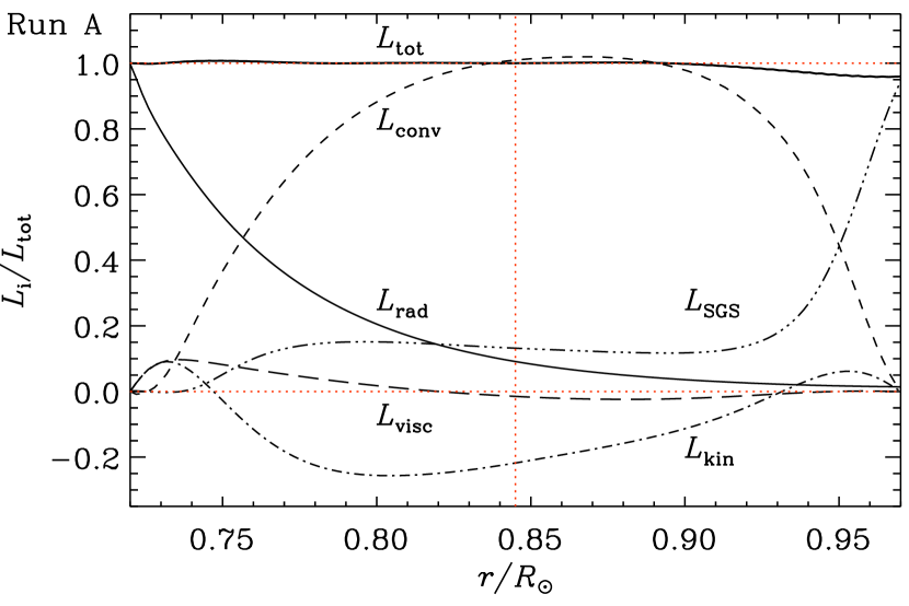
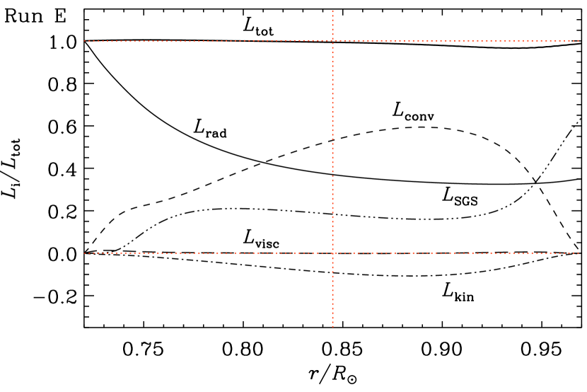
Figure 2: Time-averaged energy fluxes from Runs A (top) and E (bottom): radiative (thin solid line), convective (dashed), kinetic energy (dash-dotted), SGS (triple-dash-dotted), and viscous (long-dashed) flux. The thick solid line denotes the total flux, whereas the red horizontal dotted lines show the zero and unity line. The red vertical dotted line at $r=r_{\rm m}$ shows the midpoint of the convection zone.

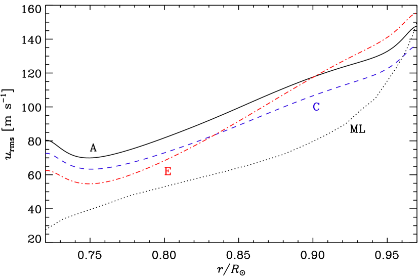
Figure 3: Radial dependence of the time averaged fluctuating rms-velocity where the contributions from the mean flows are omitted for Runs A (solid black line), C (blue dashed), and E (red dot-dashed). The black dotted line shows the convective velocity from the mixing length (ML) model of Stix (2002).

3 Results

Our simulations are summarized in Table 1. We perform three sets of runs. In the first set, we run the model from the initial conditions described in Sect. 2.1 (Runs A–E). Here, Runs A–C turn out to have anti-solar differential rotation, while Runs D and E have solar-like differential rotation. Secondly, we study the bistability of the rotation profile by taking either a solar-like (Runs D0–D4) or an anti-solar (Runs B0–B10b) solution as initial conditions. Apart from $\delta n$, we keep all other parameters fixed. We also estimate $\Lambda$ effect coefficients from the simulation results.

3.1 Effect of varying radiative flux

We change the radiative conductivity by varying the parameter $\delta n$, which regulates the amount of flux that convection has to transport, thus influencing the convective velocities and the Coriolis number. The different contributions to the total energy flux from Runs A and E are shown in Fig. 2. The definitions of the fluxes can be found in Käpylä et al. (2013). We give the fractions of convective and radiative contributions to the total energy flux at the middle of the convection zone in Table 1. For $\delta n=2.5$ (Run A) the convective flux can exceed the total flux, so the radiative flux transports less than 10 per cent of the luminosity in the upper part of the convection zone. In Run E with $\delta n=1.75$ the fractions of radiative diffusion and convection are 37 and 53 per cent, respectively. In the extreme case of $\delta n=1$ (Runs B10 and B10b), convection transports only about 20 per cent of the flux. These cases are comparable to the setups used in earlier works (Käpylä et al. 2010b, 2011b).

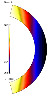
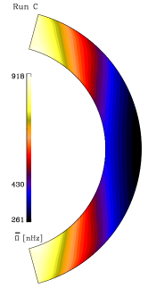
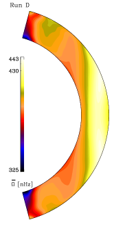
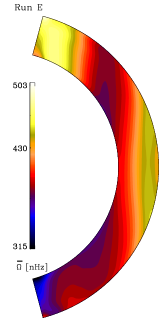
Figure 4: Time-averaged rotation profiles from Runs A–E showing $\overline{\Omega}$ in nHz.

The rms-velocities based on the fluctuating velocity for Runs A, C, and E are shown in Fig. 3. The changes between Runs A and C are rather subtle, the main effect being the decrease in the overall magnitude of $u_{\rm rms}$. The main difference between Runs C and E is the increased contrast of the values near the boundaries. We also find that all runs show higher velocities than the mixing length (ML) model of Stix (2002) below $r=0.95R_{\odot}$. The increase in $u_{\rm rms}$ near the lower boundary is due to our impenetrable boundary condition. Near the upper boundary our values of $u_{\rm rms}$ are close to those obtained from ML. A likely explanation is the weaker density stratification used in our simulations ($\Gamma\approx 12$) as opposed to what is realized in the ML model ($\Gamma\approx 60$), leading to higher values near the surface in the latter. Computing an average velocity using the data in Fig. 3 and using that to compute a Coriolis number according to Eq. (18), we find ${\rm Co}\approx 2.13$ for the ML model. This is clearly above the values for our Runs A–E owing to the lower velocities. However, we note that recent high-resolution simulations of non-rotating solar convection suggest significantly higher velocities than anticipated from ML models (Hotta et al. 2014) so the actual Coriolis number of the Sun might also be much smaller than our estimate.

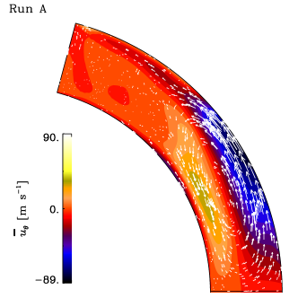
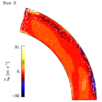
Figure 5: Time-averaged meridional circulation from Runs A (left) and D (right). The arrows show the flow $\overline{\bm{u}}_{\rm m}=(\overline{u}_{r},\overline{u}_{\theta})$, whereas the colour contours show $\overline{u}_{\theta}$.

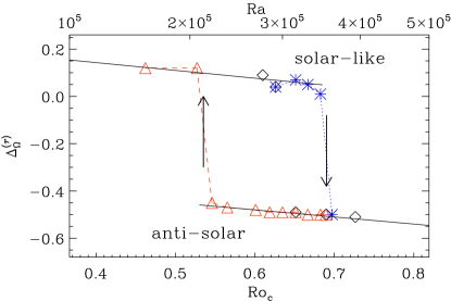
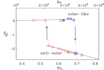
Figure 6: Radial (left panel) and latitudinal (right panel) differential rotation, defined by Eqs. (21), from Runs A–E (diamonds), and Set D (blue dotted line with asterisks) and B (red dashed line with triangles).

3.2 Differential rotation

The decrease in the rms-velocity, since $\delta n$ is lowered, is also reflected in the Coriolis number, which more than doubles between the extreme cases A and B10. The increasing rotational effect on the flow affects the rotation profile realized in the runs. The profiles of $\overline{\Omega}=\overline{u}_{\phi}/r\sin\theta+\Omega_{0}$ are shown in Fig. 4 for Runs A–E, which were run from the initial conditions stated in Sect. 2.1 with $\delta n$ varying systematically. We characterize the relative radial and latitudinal differential rotation by the quantities (Käpylä et al. 2013)

$$\Delta_{\Omega}^{(r)}=\frac{\Omega_{\rm eq}-\Omega_{\rm bot}}{\Omega_{\rm eq}},\quad\Delta_{\Omega}^{(\theta)}=\frac{\Omega_{\rm eq}-\Omega_{\rm pole}}{\Omega_{\rm eq}},$$ (21)

where $\Omega_{\rm eq}=\overline{\Omega}(r_{1},\pi/2)$ and $\Omega_{\rm bot}=\overline{\Omega}(r_{0},\pi/2)$ are the equatorial rotation rates at the surface and at the base of the convection zone, and $\Omega_{\rm pole}={\textstyle{1\over 2}}[\overline{\Omega}(r_{1},\theta_{0})+\overline{\Omega}(r_{1},\pi-\theta_{0})]$ is the average rotation rate between the latitudinal boundaries on the outer radius. In the Sun, $\Delta_{\Omega}^{(r)}>0$ and $\Delta_{\Omega}^{(\theta)}>0$, which is what is required for a solution to be classified as ‘solar-like’.

For high values of $\delta n$, i.e. for low radiative flux (Runs A–C), the rotation profile is anti-solar with a negative radial gradient of $\overline{\Omega}$ at all latitudes. The difference $\Delta\overline{\Omega}$ between the equator and latitudes $\pm 75\degr$ is larger than $1.5\Omega_{\odot}$ in both cases. In Run D the rotation profile flips to solar-like. Thus, the transition from the anti-solar to solar-like regime occurs when $1.85<\delta n<2.0$, corresponding to $1.33<{\rm Co}<1.50$ in this set of runs. This is compatible with the results of Gastine et al. (2014), who found the transition at a local Rossby number of around ${\rm Ro}_{l}\approx 1$ where ${\rm Ro}_{l}\approx 2/{\rm Co}$. As noted by Gastine et al. (2014), the transition is abrupt and occurs in a narrow parameter range. In Runs D and E, with the highest Coriolis numbers, the rotation profile is clearly solar-like. However, there are some interesting features in Run E: a strong polar jet appears on the northern hemisphere, and a decrease in $\overline{\Omega}$ is seen near the equator. Such polar vortices have frequently been found in similar simulations, see, e.g., Käpylä et al. (2010b, 2011b, 2011a), and were also found in rapidly rotating convection in relatively thin shells (e.g. Elliott et al. 2000; Gastine & Wicht 2012). In the current setup this tendency is weaker, but we still occasionally observe polar jets (Runs E, B9, and B10; see also the left panel of Fig. 9.

We note that Run A is expected to be closest to the Sun with the highest convective energy flux. Furthermore, our choice of ${\rm Pr}_{\rm SGS}=0.25$ leads to a fairly large contribution of SGS-flux within the convection zone, which in the Sun is transported by convection. These results imply that the convective velocities in the Sun would be even higher, leading to lower ${\rm Co}$ and conditions that are more suitable for anti-solar differential rotation. There are, however, hints that the velocities in simulations might be significantly higher than those in the Sun (cf. Hanasoge et al. 2012; Miesch et al. 2012).

3.3 Meridional circulation

Figure 5 shows the meridional circulation from representative Runs A and D. In the relatively slowly rotating anti-solar Run A, the flow is concentrated in a single anti-clockwise cell mostly outside the tangent cylinder with a peak amplitude of $90$ m s^-1, which is clearly higher than what is observed in the Sun (e.g. Zhao & Kosovichev 2004). In Run D the circulation pattern extends to higher latitudes and consists of several cells at low latitudes. The cell at high latitudes is likely an artefact of the closed $\theta$-boundary. A similar transition from multiple to single cells has been observed before in different settings (e.g. Käpylä et al. 2011a; Matt et al. 2011; Gastine et al. 2013). The flow amplitude near the surface in Run D is of the order of $30\,{\rm m}\,{\rm s}^{-1}$, which is still somewhat higher than the $20\,{\rm m}\,{\rm s}^{-1}$ obtained from helioseismology (Zhao & Kosovichev 2004).

A single-cell poleward circulation with solar-like rotation has been reported from simulations in spherical shells with the ASH code by imposing a latitudinal entropy variation on the bottom boundary (Miesch 2007; Miesch et al. 2011). In our spherical-wedge simulations, such a circulation pattern in combination with a solar-like differential rotation profile has so far occurred only as a transitory phenomenon in runs that have not yet fully relaxed, and they typically end up in the anti-solar regime. Recent helioseismic studies suggest that the solar meridional circulation pattern consists of several cells in radius and possibly also in latitude (Zhao et al. 2013; Schad et al. 2013; Kholikov et al. 2014), which is also realized in our more rapidly rotating cases but is at odds with mean-field models of solar rotation (e.g. Rempel 2005; Kitchatinov & Rüdiger 2005).

3.4 Flow bistability

We confirm recent results of Gastine et al. (2014) that near the transition from solar-like to anti-solar differential rotation, two stable solutions for the large-scale flow exist for the same parameter values, only depending on the initial conditions.

Our results for $\Delta_{\Omega}^{(r)}$ and $\Delta_{\Omega}^{(\theta)}$ are shown in Fig. 6 for three sets of models (cf. Table 1). Firstly, we run models from the initial conditions described in Sect. 2.1. Furthermore, we run two additional sets where we take a snapshot from an anti-solar and a solar-like solution as initial conditions. In the last two sets we vary the Rayleigh and Prandtl numbers by changing $\delta n$ and hence the radiative conductivity $K(r)$, while keeping the other control parameters at fixed values. We find that for these choices of parameters and initial conditions, it is more difficult to switch from anti-solar to solar-like differential rotation than vice versa. This is seen by comparing the $\delta n$ required for solar-like solutions in the different sets of runs: in Set D where we approach from the rapid rotation regime, the switch occurs between $0.68<{\rm Ro}_{\rm c}<0.70$ ($1.27<{\rm Co}<1.37$). In the opposite case of Set B, where we approach from the anti-solar branch, the switch occurs between $0.53<{\rm Ro}_{\rm c}<0.55$ ($2.43<{\rm Co}<2.01$). In the case of Runs A–E that were run from scratch, we found $0.63<{\rm Ro}_{\rm c}<0.65$ ($1.33<{\rm Co}<1.50$). Thus, in terms of the Coriolis number the bistability region extends farther into the anti-solar regime than the solar-like one. Physically, this might be related to the fact that in this case the strength of the differential rotation is much larger (see the two panels of Fig. 6). We have considered a single value of the Taylor number in our study. We note that according to Gastine et al. (2014), the size of the bistable region is wider with higher ${\rm Ta}$.

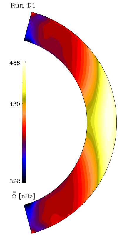
Figure 7: Time-averaged rotation profiles from Runs C and D1.

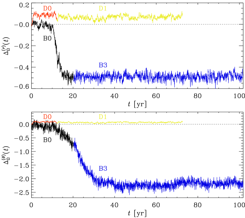
Figure 8: Radial and latitudinal differential rotation as functions of time from Runs D1 and B3 with the same parameters.

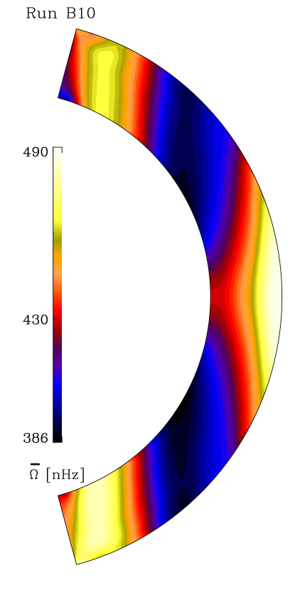
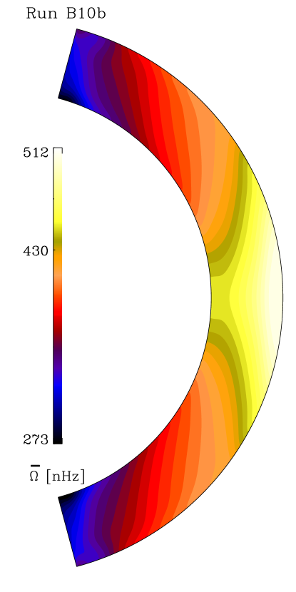
Figure 9: Time-averaged rotation profiles from Runs B10 and B10b.

Figure 7 shows the rotation profiles from Runs C and D1 that have the same control parameters but different histories: Run C was run from the initial conditions described in Section 2.1, whereas in Run D1 we used the final thermally relaxed state of Run D (=D0) as initial condition. The resulting evolution of $\Delta_{\Omega}^{(r)}$ and $\Delta_{\Omega}^{(\theta)}$ is shown in Fig. 8, where we also show the corresponding results for Run B3 with the same input parameters as Run D1 after restarting from Run B (=B0). Our simulations were typically run for roughly 100 years solar time. By comparison, the viscous and SGS diffusion times, $\tau_{\nu}=(\Delta r)^{2}/\nu$ and $\tau_{\rm SGS}=\tau_{\nu}{\rm Pr}_{\rm SGS}$, in our simulations are $10.5$ and $2.6$ years, respectively.

Rapidly rotating toroidal jets at high latitudes appear in many numerical simulations of global scale convection (e.g. Miesch et al. 2000; Käpylä et al. 2011a, b). In the Sun the latitudinal gradient of $\overline{\Omega}$ is known to be monotonic in each hemisphere. Models based on solar differential rotation have also been adopted in stellar studies where low latitude bands or polar vortices are ignored. Non-magnetic mean-field models also tend to produce this type of solution. However, the gas giants in the solar system have alternating bands of slower and faster rotation, although in that case it is not clear whether the convective layer is deep (e.g. Busse 1976; Heimpel & Aurnou 2007) or shallow (Kaspi et al. 2013). There are also theoretical and observational studies suggesting similar profiles for fully convective M-dwarfs and brown dwarfs (e.g. Balbus & Weiss 2010; Crossfield et al. 2014).

In Figure 9 we show the rotation profiles obtained in Runs B10 and B10b with the same control parameters. Run B10 was run from a snapshot of Run B0 exhibiting anti-solar differential rotation. This run now exhibits polar jets. However, it has been suggested that these jets can be unstable (Wicht et al. 2002). To investigate this possibility further, we take a snapshot from B10 as initial for Run B10b and apply a relaxation term at high latitudes for the azimuthally averaged $u_{\phi}$ that yields a monotonic latitudinal gradient of $\overline{\Omega}$. The relaxation timescale is roughly four days and the term is switched on for two weeks in solar time in the beginning of the simulation. We find that the resulting profile with a more solar-like monotonic behaviour is also stable—at least for 50 years, which corresponds to roughly five viscous diffusion times.

3.5 $\Lambda$ effect and turbulent viscosity

The changes in the differential rotation should somehow be reflected in similar changes in the underlying mechanism responsible for driving it, which is the $\Lambda$ effect (Rüdiger 1980, 1989). The $\Lambda$ effect corresponds to a rank three tensor that parameterizes the non-diffusive contributions to the Reynolds stress, in addition to the diffusive contributions that result from turbulent viscosity. The Reynolds stress is given by $Q_{ij}=\overline{u_{i}^{\prime}u_{j}^{\prime}}$, where $\bm{u}^{\prime}=\bm{u}-\overline{\bm{u}}$ is the fluctuating velocity. The relevant off-diagonal components can be written as

$$Q_{r\phi} = \Lambda_{\rm V}\sin\theta\overline{\Omega}-\nu_{\rm t}r\sin\theta\frac{\partial\overline{\Omega}}{\partial r},$$ (22)

$$Q_{\theta\phi} = \Lambda_{\rm H}\cos\theta\overline{\Omega}-\nu_{\rm t}\sin\theta\frac{\partial\overline{\Omega}}{\partial\theta},$$ (23)

where $\Lambda_{\rm V}$ and $\Lambda_{\rm H}$ are the vertical and horizontal components of the $\Lambda$ effect and $\nu_{\rm t}$ is the turbulent viscosity. Obviously, we cannot extract both effects self-consistently from a single Reynolds stress component. Instead, we use a simple mixing length formula to estimate the turbulent viscosity

$$\nu_{\rm t}={\textstyle{1\over 3}}u_{\rm rms}\alpha_{\rm MLT}H_{p},$$ (24)

where $u_{\rm rms}=u_{\rm rms}(r,\theta)$ varies across the meridional plane, $\alpha_{\rm MLT}=1.7$ is taken for the mixing length parameter, and $H_{p}=-(\partial\ln p/\partial r)^{-1}$ is the pressure scale height. Similar methods have been applied in earlier studies of isotropically forced turbulence (Snellman et al. 2009) and convection (Pulkkinen et al. 1993; Käpylä et al. 2010a) in Cartesian geometry, where anisotropy is self-consistently produced by rotation and/or stratification. In Fig. 10 we present the results for Runs A and D, which are representative of anti-solar and solar-like rotation regimes.

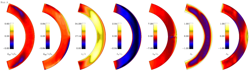
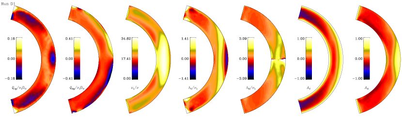
Figure 10: From left to right: Time-averaged Reynolds stresses $Q_{r\phi}$ and $Q_{\theta\phi}$ normalized by $\nu_{\rm t}\Omega_{\odot}$, the turbulent viscosity divided by the molecular viscosity $\nu_{\rm t}/\nu$, $\Lambda_{\rm V}$ and $\Lambda_{\rm H}$ normalized by $\nu_{\rm t}$, and the anisotropy parameters $A_{\rm V}$ and $A_{\rm H}$. Top row: Run A; bottom row: Run D1. In the fifth column we only use data some degrees away from the equator so as to avoid the singularity associated with the division by $\cos\theta$. The contours in the lower row are oversaturated near the $\theta$-boundaries in order to highlight the features at lower latitudes.

In both cases, the Reynolds stress responsible for radial transport of angular momentum, $Q_{r\phi}$, is negative at high latitudes. Somewhat surprisingly, $Q_{r\phi}$ is very small near the equator in the relatively slowly rotating Run A, but consistent with early results of Rieutord et al. (1994). In Run D1, in the solar-like regime, a positive contribution to the stress appears at low latitudes. The latter is consistent with Cartesian simulations where the corresponding stress changes sign at low latitudes in the rapid rotation regime (Käpylä et al. 2004). The horizontal stress, $Q_{\theta\phi}$, leads to angular momentum transport that is directed toward the equator in both runs, except at high latitudes in Run A where the transport is toward the poles.

The mixing length estimate of the turbulent viscosity shows a decrease at high latitudes in comparison to the equatorial regions in Run A. In Run D1 there is a minimum at mid-latitudes. In both cases the maximum value of $\nu_{\rm t}/\nu$ is of the order of 35, which is reasonable given that the Reynolds numbers in both runs are similar. We have here neglected anisotropies that are caused by gravity and rotation that play the roles of preferred directions in the system. Thus, we do not expect the details of the turbulent viscosity to be captured accurately. However, the order of magnitude of $\nu_{\rm t}/\nu\approx{\rm Re}$ seems reasonable, so we proceed to using this estimate to extract the $\Lambda$ effect.

Solving Eqs. (22) and (23) for $\Lambda_{\rm V}$ and $\Lambda_{\rm H}$ yields

$$\Lambda_{\rm V} = \frac{Q_{r\phi}}{\sin\theta\;\overline{\Omega}}+\nu_{\rm t}r\frac{\partial\ln\overline{\Omega}}{\partial r},$$ (25)

$$\Lambda_{\rm H} = \frac{Q_{\theta\phi}}{\cos\theta\;\overline{\Omega}}+\nu_{\rm t}\tan\theta\frac{\partial\ln\overline{\Omega}}{\partial\theta}.$$ (26)

The profiles of $\Lambda_{\rm V}$ show some distinct differences between both runs. It is mostly negative for the anti-solar Run A and mostly positive for the solar-like Run D1. Interestingly, these differences would not have been so obvious if we had directly compared the vertical stresses $Q_{r\phi}$ of both runs. This highlights the usefulness of employing Eq. (25), even though this involves the uncertainty of estimating $\nu_{\rm t}$. Likewise, while the horizontal stresses $Q_{\theta\phi}$ for Runs A and D1 show some similarities, the profiles of $\Lambda_{\rm H}$ also show differences between both runs, and it is mostly negative for the anti-solar Runs A and mostly positive for the solar-like Run D1.

According to mean-field theory (Rüdiger 1980), coefficients $\Lambda_{\rm V}$ and $\Lambda_{\rm H}$ are related to the anisotropy parameters

$$A_{\rm V}=\frac{Q_{\phi\phi}-Q_{rr}}{Q_{\phi\phi}+Q_{rr}},\ \ \ A_{\rm H}=\frac{Q_{\phi\phi}-Q_{\theta\theta}}{Q_{\phi\phi}+Q_{\theta\theta}},$$ (27)

via $\Lambda_{\rm V}\approx 2\tau A_{\rm V}$ and $\Lambda_{\rm H}\approx 2\tau A_{\rm H}$, where $\tau$ is the correlation time of the turbulence. Profiles of $A_{\rm V}$ and $A_{\rm H}$ are shown in the last two columns of Fig. (10). In Run A, both $\Lambda_{\rm V}$ and $A_{\rm V}$ are mostly negative, while both are mostly positive for Run D1, in broad agreement with the radial differential rotation gradient. Also $\Lambda_{\rm H}$ and $A_{\rm H}$ are mostly negative in Run A and mostly positive in Run D1, again in broad agreement with the latitudinal differential rotation.

According to first-order smoothing results (e.g. Kitchatinov & Rüdiger 1995, 2005), $A_{\rm V}$ is always negative due to the simplified turbulence model used. This, however, is not always the case in simulations (e.g. Käpylä et al. 2004). Indeed, $A_{\rm V}$ is mostly negative in Run A and attains positive values near the equator in Run D1, in qualitative accordance to our estimates of $\Lambda_{\rm V}$ for each case. Similarly we find that the sign of $A_{\rm H}$ agrees mostly with that of $\Lambda_{\rm H}$. It is remarkable that the results for the $\Lambda$ effect are consistent with those of the anisotropy parameters given our use of a very simple approximation for $\nu_{\rm t}$. Our results for $A_{\rm V}$ and $A_{\rm H}$ also indicate that the differential rotation has a significant impact on the properties of turbulence.

For the run with solar-like rotation (Run D), $\Lambda_{\rm H}$ is concentrated near the equator and close to the upper boundary. A similar concentration near the equator has also been observed in earlier studies (e.g. Chan 2001; Käpylä et al. 2004) and can be partly explained by the banana cells near the equator (Käpylä et al. 2011b).

4 Conclusions

Simulations of mildly turbulent three-dimensional convection in spherical wedges have allowed us to study aspects of differential rotation relevant to the Sun. In our most solar-like model, Run A, we found anti-solar differential rotation. Decreasing the convective velocities by increasing the radiative conductivity, thereby also increasing the Coriolis number, we found a threshold after which the rotation changes to a solar-like profile. In agreement with the recent finding of Gastine et al. (2014) using Boussinesq convection, our stratified and compressible models near the threshold between both states confirm the existence of bistability in that the question of anti-solar or solar-like rotation depends on the initial condition or the history of the run. We also confirmed earlier findings showing that high-latitude toroidal jets are possible in runs where solar-like solutions are observed with the same parameters. This could be significant for stellar rotation profiles that are naively assumed to have a monotonic latitudinal gradient of angular velocity. These jets may well be asymmetric and present only at one of the poles (see also Heimpel & Aurnou 2007; Jones & Kuzanyan 2009).

Another interesting but speculative conjecture is that the solar differential rotation is also the result of bistability. Our Runs A and B with energy fluxes closest to what we would expect from the Sun i.e. where resolved convection transports most of the total flux, show anti-solar differential rotation. Making the model more realistic with respect to the Sun requires that we (i) decrease the SGS-flux, which now contributes more than ten per cent of the total, (ii) increase the density stratification by a factor of five, and (iii) increase the Reynolds number. All of these factors are likely to lead to higher convective velocities and thus lower Coriolis number, in turn leading to even more suitable conditions for anti-solar differential rotation. We know, however, that the Sun rotated much more rapidly in its youth, which favours a solar-like rotation profile. Furthermore, the results of Gastine et al. (2014) suggest that the range of parameters in which bistable solutions are possible increases as the Taylor number increases. These two facts lend some credence to the conjecture that the Sun is in a bistable regime. Clearly, further research into this matter is required.