Bayesian analysis for a class of beta mixed models

Abstract

Generalized linear mixed models (GLMM) encompass large class of statistical models, with a vast range of applications areas. GLMM extends the linear mixed models allowing for different types of response variable. Three most common data types are continuous, counts and binary and standard distributions for these types of response variables are Gaussian, Poisson and Binomial, respectively. Despite that flexibility, there are situations where the response variable is continuous, but bounded, such as rates, percentages, indexes and proportions. In such situations the usual GLMM’s are not adequate because bounds are ignored and the beta distribution can be used. Likelihood and Bayesian inference for beta mixed models are not straightforward demanding a computational overhead. Recently, a new algorithm for Bayesian inference called INLA (Integrated Nested Laplace Approximation) was proposed. INLA allows computation of many Bayesian GLMMs in a reasonable amount time allowing extensive comparison among models. We explore Bayesian inference for beta mixed models by INLA. We discuss the choice of prior distributions, sensitivity analysis and model selection measures through a real data set. The results obtained from INLA are compared with those obtained by an MCMC algorithm and likelihood analysis. We analyze data from an study on a life quality index of industry workers collected according to a hierarchical sampling scheme. Results show that the INLA approach is suitable and faster to fit the proposed beta mixed models producing results similar to alternative algorithms and with easier handling of modeling alternatives. Sensitivity analysis, measures of goodness of fit and model choice are discussed.

1 Introduction

There has been an increased interest in the class of Generalized Linear Mixed Models (GLMM). One possible reason for such popularity is that GLMM combine Generalized Linear Models (GLM) (Nelder and Wedderburn, 1972) with Gaussian random effects, adding flexibility to the models and accommodating complex data structures such as hierarchical, repeated measures, longitudinal, among others which typically induce extra variability and/or dependence.

GLMMs can also be viewed as natural extension of Mixed Linear Models (Pinheiro and Bates, 2000), allowing a wider class of probability distributions for response variables. Common choices are Gaussian for continuous data, Poisson and Negative Binomial for count data and Binomial for binary data. These three situations include the majority of applications within this class of models. Examples can be found in (Breslow and Clayton, 1993) and (Molenberghs and Verbeke, 2005).

Despite that flexibility, there are situations where the response variable is continuous and bounded above and below such as rates, percentages, indexes and proportions. In such situations the traditional GLMM based on the Gaussian distribution, is not adequate, since bounding is ignored. An approach that has been used to model this type of data is based on the beta distribution. The beta distribution is very flexible with density function that can display quite different shapes, including left or right skewness, symmetric, J-shape, and inverted J-shape (da Silva et al., 2011).

Regression models for independent and identically distributed beta variable proposed by Paolino (2001), Kieschnick and McCullough (2003) and Ferrari and Cribari-Neto (2004). The basic assumption is that the response follow a beta law whose expected value is related to a linear predictor through a link function, similarly to GLM’s. Cepeda (2001), Cepeda and Gamerman (2005) and Simas et al. (2010) extend the model regressing both, the mean and the precision parameters with covariates. Smithson and Verkuilen (2006) explores beta regression with an application to IQ data. Methods for likelihood based inference and model assessment are proposed by Espinheira et al. (2008b), Espinheira et al. (2008a) and Rocha and Simas (2011). Bias corrections for likelihood estimators are developed by Ospina et al. (2006), Ospina et al. (2011) and Simas et al. (2010). Branscum et al. (2007) adopts Bayesian inference to analyze virus genetic distances. Recently, Bonat et al. (2012) contrasted beta regression models with other approaches to model response variable on the unity interval, such that, Simplex, Kumaraswamy and Trans-Gaussian models. Results show there is no overall prominent model.

The beta regression is implemented by betareg package (Cribari-Neto and Zeileis, 2010) for the R environment for statistical computing (R Development Core Team, 2012). Extended functionality is added for bias correction, recursive partitioning and latent finite mixture (Grün et al., 2012). Mixed and mixture models are further discussed by Verkuilen and Smithson (2012).

For non independent data, development have been proposed in times series analysis by McKenzie (1985), Grunwald et al. (1993) and Rocha and Cribari-Neto (2008). da Silva et al. (2011) use a Bayesian beta dynamic model for modeling and prediction of time series with an application to the Brazilian unemployment rates. Figueroa-Zúñiga et al. (2013) extend the beta model proposed by Ferrari and Cribari-Neto (2004) using a Bayesian approach. The authors considered two distributions for the random effects (Gaussian and t-Student) and several specifications for the prior distributions for parameters in the model.

Bonat et al. (2013) extend the beta model proposed by Ferrari and Cribari-Neto (2004) with the inclusion of Gaussian random effects, under a GLMM approach. Likelihood inference is based on two algorithms. The first uses the Laplace approximation to solve the integral in the likelihood function and the second uses an algorithm proposed by Lele et al. (2010) called data cloning. Authors analyzed two real data sets, with different structures for the random effects. Likelihood inference under GLMM is non-trivial because of presence random effects and several procedures have been proposed. Approximate likelihood methods are adopted by Breslow and Clayton (1993) and a Monte Carlo approach is adopted by Chen et al. (2002). Both come with a computational overhead. A popular approach is based upon a Bayesian framework using Markov Chain Monte Carlo (MCMC) algorithms with attempts to set non informative priors. Figueroa-Zúñiga et al. (2013) perform Bayesian inference for beta mixed models using an MCMC algorithm. The Bayesian approach is attractive but requires specification of prior distributions, which is not straightforward, in particular for variance components.

Recently, Rue et al. (2009) introduced a novel numerical inference approach, the so-called Integrated Nested Laplace Approximation (INLA). INLA allows the computation of many Bayesian GLMMs in a reasonable amount of time, enabling for extensive comparisons of different models and prior distributions. Fong et al. (2010) used INLA for Bayesian analysis of several data sets and concluded that INLA is a very accurate algorithm and present results which help to guide the choice of prior distributions.

The main goal this paper is describe Bayesian inference for beta mixed models using INLA. We discuss the choice of prior distributions and measures of model comparisons. Results obtained from INLA are compared to those obtained using a Bayesian MCMC algorithm and a purely likelihood analysis. The modelling is illustrated through the analysis of a real dataset from a study on a life quality index of industry workers, with data collected according to a hierarchical sampling scheme. Additional care is given to choice of prior distributions for precision parameter of the beta law.

The structure this paper is the follows. In Section 2, we define the Bayesian beta mixed model, Section 3 we describe the Integrated Nested Laplace Approximation (INLA). In Section 4 the model is introduced for the motivating example and the results of the analyses are presented. We close with concluding remarks in Section 5.

2 Bayesian beta mixed model

Bayesian beta mixed regression extends the beta regression model, as proposed by Ferrari and Cribari-Neto (2004), by adding Gaussian distributed random effects to the linear predictor. Consider the response $Y_{ij}$ from group $i=1,\ldots,N$ and replication $j=1,\ldots,n_{i}$. $\mathbf{Y}_{i}$ is a $n_{i}-dimensional$ vector of measurements on the $i^{th}$ group. Given a $q$-dimensional vector $\mathbf{b_{i}}$ of random effects distributed as $N(\mathbf{0},Q(\boldsymbol{\tau}))$, the responses $Y_{ij}$ are conditionally independent with density function given by

$$\pi_{i}(y_{ij}|\mathbf{b_{i}},\mu_{ij},\phi)=\frac{\Gamma(\phi)}{\Gamma(\mu_{ij}\phi)\Gamma((1-\mu_{ij})\phi)}y_{ij}^{\mu_{ij}\phi-1}(1-y_{ij})^{(1-\mu_{ij})\phi-1},\quad 0<y<1,$$ (1)

where $0<\mu<1$ is the mean of the response variable and $\phi>0$ is a dispersion parameter. Let $g(.)$ be a known link function with $g(\mu_{ij})=\mathbf{x}_{ij}^{T}\boldsymbol{\beta}+\mathbf{z}_{ij}^{T}\mathbf{b_{i}}$, where $\mathbf{x}_{ij}$ and $\mathbf{z}_{ij}$ are vectors of covariates with dimensions $p$ and $q$, respectively, and $\boldsymbol{\beta}$ is a $p$-dimensional vector of unknown regression parameters. Assume that $\mathbf{b_{i}}|Q(\boldsymbol{\tau})\sim N(\mathbf{0},Q(\boldsymbol{\tau})^{-1})$, where the precision matrix $Q(\boldsymbol{\tau})$ depends on parameters $\boldsymbol{\tau}$. The model specification is completed assuming prior distributions for all parameters in the model, say $\mathbf{\theta}=(\boldsymbol{\beta},\phi,\boldsymbol{\tau})$.

A flat improper prior is assumed for the intercept $\beta_{0}$. All other components of $\boldsymbol{\beta}$ are assumed to be independent $N(0,\sigma^{2})$ with fixed precision $\sigma^{-2}=0.0001$. For the parameters in the precision matrix $(\boldsymbol{\tau})$ we follow an approach adopted by Fong et al. (2010) based on Wakefield (2009). The basic idea is to specify a range for the more interpretable marginal distribution of $b_{i}$ and use this to derive the specification of the prior distributions. The approach is based on the result that if $b|\tau\sim N(0,\tau^{-1})$ and $\tau\sim Ga(a_{1},a_{2})$ then $b\sim t(0,a_{2}/a_{1},2a_{1})$. To decide upon a prior, we define a range for a generic random effects $b$ and specify the degrees of freedom, $d$, and then solve for $a_{1}$ and $a_{2}$. The solution for a generic range, say $(-R,R)$, is $a_{1}=d/2$ and $a_{2}=R^{2}d/(2(t_{1-(1-q)/2}^{d}))^{2}$. In linear mixed effects model, $b$ is directly interpretable, while for beta models, it is more appropriate to think in terms of the marginal distribution of $exp(b)$. The prior distributions obtained this way are flat. For more detailed description see Fong et al. (2010) section $4.2$.

A flat $Ga(a_{1}=1,a_{2}=0.001)$ prior is choosen for $\phi$ as no result is known to aid its specification. The sensitivity to prior assumptions on the precision parameters of the beta distribution and of the random effects is a potentially a delicate issue under beta mixed models. Figueroa-Zúñiga et al. (2013) considers several choices of prior distributions to $\phi$ but no sensitivity analysis is performed. The idea here is to specify this Gamma distribution as the default choice and then to assess the sensitivity.

3 Inference, model selection and sensitivity

Bayesian inference on beta mixed models is not straightforward since the posterior distribution is not analytically available. Markov Chain Monte Carlo (MCMC) technique is the standard approach to fit such models (Figueroa-Zúñiga et al., 2013). In practice, this approach comes with a wide range of problems in terms of convergence and computational time. Moreover, the implementation itself can be problematic, especially for end users who might not be experts in programming. Software platforms for fitting generic random effects models via MCMC, include JAGS (Plummer, 2003), BayesX (Belitz et al., 2012) and WinBUGS (Lunn et al., 2000), among others.

Rue et al. (2013 +0100) is a newer tool for an end user based on the INLA (Integrated Nested Laplace Approximation) approach for Bayesian inference on latent Gaussian models with focus on the posterior marginal distributions (Rue et al., 2009). INLA replaces MCMC simulations by accurate deterministic approximations to posterior marginal distributions.

A computational implementation called inla, available at http://www.r-inla.org, allows the user to conveniently perform approximate Bayesian inference in latent Gaussian models. The R package INLA serves as an interface to inla routines and its usage is similar to the glm function in R (Roos and Held, 2011). Standard output provides marginal posterior densities for all parameters in the model and several measures of model goodness of fit.

The procedure of statistical analysis of a real data set, consists of specify the model, parameter estimation, comparisons among several models and evaluation results sensitivity, given the model specification. The second is tackled by INLA, and then the output includes several measures of model goodness of fit. The three more useful are, the Deviance Information Criterion (DIC), the log marginal likelihood (LML) and the conditional predictive ordinate (CPO), for more details, see Roos and Held (2011).

Roos and Held (2011) develop a general sensitivity measure based on the Hellinger distance to assess sensitivity of the posterior distributions with respect to changes on the prior distributions for precision parameters. Such methods is adopted here to assess the sensitivity to the choice of the prior distribution for $\phi$ and for the precision of the random effects. Following Roos and Held (2011), for a default $\boldsymbol{\theta}_{0}$ and a shifted $\boldsymbol{\theta}$ prior value let

$$S(\boldsymbol{\theta}_{0},\boldsymbol{\theta})=\frac{H(post(\boldsymbol{\theta}_{0}),post(\boldsymbol{\theta}))}{H(pri(\boldsymbol{\theta}_{0}),pri(\boldsymbol{\theta}))}$$ (2)

denote the relative change on the posterior distribution with respect to changes on the prior distribution as measured by the Hellinger distance $H$, where $pri(\theta)$ is the prior distribution, $post(\theta)$ is the corresponding posterior distribution and

$$H(f,g)=\sqrt{1-BC(f,g)},\quad\text{where}\quad BC(f,g)=\int_{-\infty}^{\infty}\sqrt{f(u),g(u)}du.$$

The Hellinger distance is symmetric and measures the discrepancy between two densities $f$ and $g$. It takes a maximal value of $1$ if $BC$ is equal to $0$ and is equal to $0$ if and only if both densities are equal. The latter happens whenever the density $f$ assigns probability $0$ to every set to which the density $g$ assigns a positive probability and vice versa. For more detailed description see Roos and Held (2011).

4 Income and life quality of Brazilian industry workers

The Brazilian industry sector worker’s life quality index (IQVT, acronym in Portuguese) is computed combining 25 indicators from eight thematic areas: housing, health, education, integral health and safety in the workplace, development of skills, value attributed to work, corporate social responsibility, stimulus to engagement and performance. The index is constructed following same premises as for the united nations human development index . The resulting values are in the unit interval and the closer to one the higher the worker’s life quality in the industry.

A poll was conducted by Industry Social Service (Serviço Social da Indústria - SESI) in order to assess worker’s life quality in the Brazilian industries. The survey included $365$ companies on eight Brazilian federative units among the total of 26 states plus the Federal District. The data analysis considers two covariates related to the companies for which the impact on IQVT is of particular interest, namely, company average income and size. The first is given by the total of salaries divided by the number of workers expressing the capacity to fulfill individual basic needs such as food, health, housing and education. The second can be indirectly related to the capability of managing and providing quality of life.

The relevant question for the study and main goal here is to specify a suitable model to assess the influence of these two covariates on the IQVT. The federative unit where the company based is expected to influence the index considering varying local legislations, taxing and further economic and political conditions. This is accounted by including a random effect, regarding the eight states as a sample of the federative units.

Relations between the IQVT and the covariates income, size and with the states included in the survey are shown on Figure 1 which suggests all are potentially relevant. The income is expressed in logarithmic scale centered around the average.

Figure 1: Scatterplot and boxplot relating IQVT with (centred) log income, company size and state.

The Bayesian beta random effects model for IQVT is given by

$$Y_{ij}|\mathbf{b}_{i} \sim Beta(\mu_{ij},\phi)$$

$$g(\mu_{ij}) =(\beta_{0}+b_{i1})+\beta_{1}Medium_{ij}+\beta_{2}Small_{ij}+(\beta_{3}+b_{i2})Income_{ij}$$

$$\mathbf{b}_{i} \sim NMV(\mathbf{0},\Sigma)\mbox{ with }\Sigma=\left[\begin{array}[]{rr}1/\tau_{1}^{2}&\rho\\ \rho&1/\tau_{2}^{2}\\ \end{array}\right]$$

parametrize with $\beta_{0}$ associated with large size companies with differences $\beta_{1}$ and $\beta_{2}$ to the medium and small size, respectively. Random effects include an intercept $b_{i1}$ and a slope $b_{i2}$ associated with the covariate income. The vector of model parameters are the regression coefficients $(\beta_{0},\beta_{1},\beta_{2},\beta_{3})$, the random effects covariance parameters $(\tau_{1}^{2},\tau_{2}^{2},\rho)$ and dispersion parameter $\phi$ from beta law. The logit $g(\mu_{ij})=\log\{\mu_{ij}/(1-\mu_{ij})\}$ link function is used. The specification the Bayesian beta mixed model is completed by specifying the prior distributions for the model parameters. Following the remarks at Section $2$ a flat improper prior is assumed $\beta_{0}$. All other components of $\beta$ are assumed to be independent zero-mean $N(0,\sigma^{2})$ with fixed precision $\sigma^{-2}=0.0001$. For the parameter $\phi$ we assumed a flat $Ga(a_{1}=1,a_{2}=0.0001)$ distribution. For the parameters indexing the random effects $\Sigma=Q^{-1}$, we assumed that $Q\sim W_{q}(r,S)$, where $W_{q}(r,S)$ denote the Wishart distribution, $r$ and $S$ to be chosen as in the univariate case. Specifically, we assumed that $r=5$ and a diagonal $S$ with elements $0.001487$ and $0.005$, reducing to a $Ga(a_{1}=0.5,a_{2}=0.001487)$ when fitting the random intercept model.

A sequence of sub-models are defined in order to assess the effects of interest. Model 1 is a null model with just the intercept coefficent. Model 2 and 3 adds the covariates size and income, in this order. Model 4 and 5 adds random effects related to the States to the intercept and the income coefficient, respectively. The latter is the largest model considered here. A sequence of nested models are defined for comparison and detection of the relevant effects. Large size companies are considered as the baseline for the categorical covariate size. Table 1 shows the posterior means for the model parameters and model fitting measures given by the deviance information criterion (DIC), log marginal likelihood (LML) and conditional predictive ordinate (CPO), all obtained with INLA.

Table 1: Posterior means, LML, DIC and CPO for the fitted models.

Parameter	Model 1	Model 2	Model 3	Model 4	Model 5
$\beta_{0}$	0.35	0.45	0.43	0.40	0.40
$\beta_{1}$		-0.11	-0.09	-0.07	-0.07
$\beta_{2}$		-0.16	-0.14	-0.13	-0.14
$\beta_{3}$			0.42	0.47	0.46
$\phi$	53.92	56.44	72.16	93.37	93.28
$\tau_{1}^{2}$				63.65	90.33
$\tau_{2}^{2}$					532.73
$\rho$					0.75
Goodness-of-fit
LML	466.02	461.57	500.11	534.40	359.82
DIC	-941.11	-955.72	-1044.58	-1130.79	-1129.29
CPO	-1.29	-1.31	-1.43	-1.55	-1.55

Results for models 1-3 confirm the relevance of the covariates. The increasing values for average posterior of $\phi$, from $53.92$ on model 1 to $72.16$ on model 3, confirms further explanation of the data variability by the covariates. The random intercept clearly improves the model fit, capturing the variability of the IQVT among the states. The addition of random slope did not prove relevant. All model fitting measures favors model 4 for which we report further analysis.

Figure 2 shows posterior distributions from INLA and a MCMC output from JAGS running three chains of 500,000 samples with a burn-in of 10,000 interactions and saving one of each 100 simulations. We also compared INLA results with likelihood point estimates and profile intervals. Figure 2 suggests that all approaches produced similar results. This is also assured by the results in Table 2 where the second and third columns provide the proportion of MCMC samples which falls into the profile likelihood interval and credibility intervals from INLA, respectively. The last column is the probability between the limits of the profile likelihood interval computed on the INLA marginal distribution. These results indicates the flat prior has little impact on the respective posterior distribution. The INLA and MCMC algorithms are similar in the inferential purposes but INLA is much faster and easier to use than MCMC.

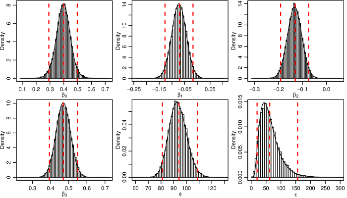
Figure 2: Marginal posterior densities from INLA and MCMC outputs. The vertical dashed lines correspond to point estimates and profile likelihood intervals.

Table 2: Comparison on the intervals obtained by different methods.

Parameter	MCMC.in.Profile	MCMC.in.INLA	Profile.in.INLA
$\beta_{0}$	0.9415	0.9435	0.9487
$\beta_{1}$	0.9457	0.9471	0.9490
$\beta_{2}$	0.9496	0.9509	0.9491
$\beta_{3}$	0.9465	0.9471	0.9491
$\phi$	0.9491	0.9510	0.9480
$\tau_{1}^{2}$	0.9446	0.9433	0.9511

We conclude the analysis assessing sensitivity to the choice the prior distributions. Following Roos and Held (2011), we investigate the sensitivity by measuring the Hellinger distance and focusing only on the parameters $\phi$ and $\tau$ since the choice of prior is standard for the regression coefficients $\beta^{\prime}s$. To assess sensitivity we choose a set of prior distributions with determined Hellinger distance from the default prior, refit the model under those priors and compute the Hellinger distances between the corresponding posterior distributions. For example, by choosing $\phi\sim Ga(b1=1,b2=0.0135)$ the Hellinger distance from the default $\phi_{0}\sim Ga(a1=1,a2=0.001)$ prior is $H(Ga(a_{1}=1,a_{2}=0.001),Ga(b_{1}=1,b_{2}=0.0135))=0.1058$ whereas the Hellinger distance between the posteriors is $0.0100$ and $S(\phi_{0},\phi)=0.0945$, i.e, the distance between the posterior distributions is only about one tenth of the distance between the prior distributions reflecting a major effect of the that and a little impact of choosing either prior. Table 3 shows the hyperparameters obtained for priors with Hellinger distances from about $0.1$ to $0.6$ and the corresponding Hellinger distances between priors, posteriors and $S(\cdot,\cdot)$. The distributions are plotted in Figure 3.

Table 3: Hellinger distances between the prior and posterior distributions from the ones obtained with the default prior.

Priori	HL Prior	HL Post	$S(post,pri)$
$\phi\sim Ga(b_{1}=1,b_{2}=0.0135)$	0.1058	0.0100	0.0945
$\phi\sim Ga(b_{1}=1,b_{2}=0.0178)$	0.2005	0.0200	0.0998
$\phi\sim Ga(b_{1}=1,b_{2}=0.0242)$	0.3005	0.0346	0.1153
$\phi\sim Ga(b_{1}=1,b_{2}=0.0338)$	0.4006	0.0583	0.1455
$\phi\sim Ga(b_{1}=1,b_{2}=0.050)$	0.5046	0.0975	0.1932
$\phi\sim Ga(b_{1}=1,b_{2}=0.0765)$	0.6004	0.1628	0.2711
$\tau\sim Ga(b_{1}=0.5,b_{2}=0.00225)$	0.1030	0.0100	0.0971
$\tau\sim Ga(b_{1}=1,b_{2}=0.0035)$	0.2086	0.0245	0.1174
$\tau\sim Ga(b_{1}=1,b_{2}=0.0055)$	0.3085	0.0458	0.1485
$\tau\sim Ga(b_{1}=1,b_{2}=0.0088)$	0.4017	0.0812	0.2022
$\tau\sim Ga(b_{1}=1,b_{2}=0.016)$	0.5031	0.1543	0.3066
$\tau\sim Ga(b_{1}=1,b_{2}=0.033)$	0.6022	0.2827	0.4694

The results show that the models are more sensitive to the choice of prior for the parameter $\tau$. For the parameter $\phi$ even with the rather large distance of 0.6 between prior distributions the corresponding distance between the posterior distributions is substantially reduced to $0.1628$. The same distance between priors for the parameter $\tau$ still reduces to $0.2827$. The posterior distributions in Figure 3 are similar for all prior distributions. Comparatively, the parameter $\tau$ is more sensitive to the choice of prior distribution, however still with similar posterior distributions even with large difference between priors.

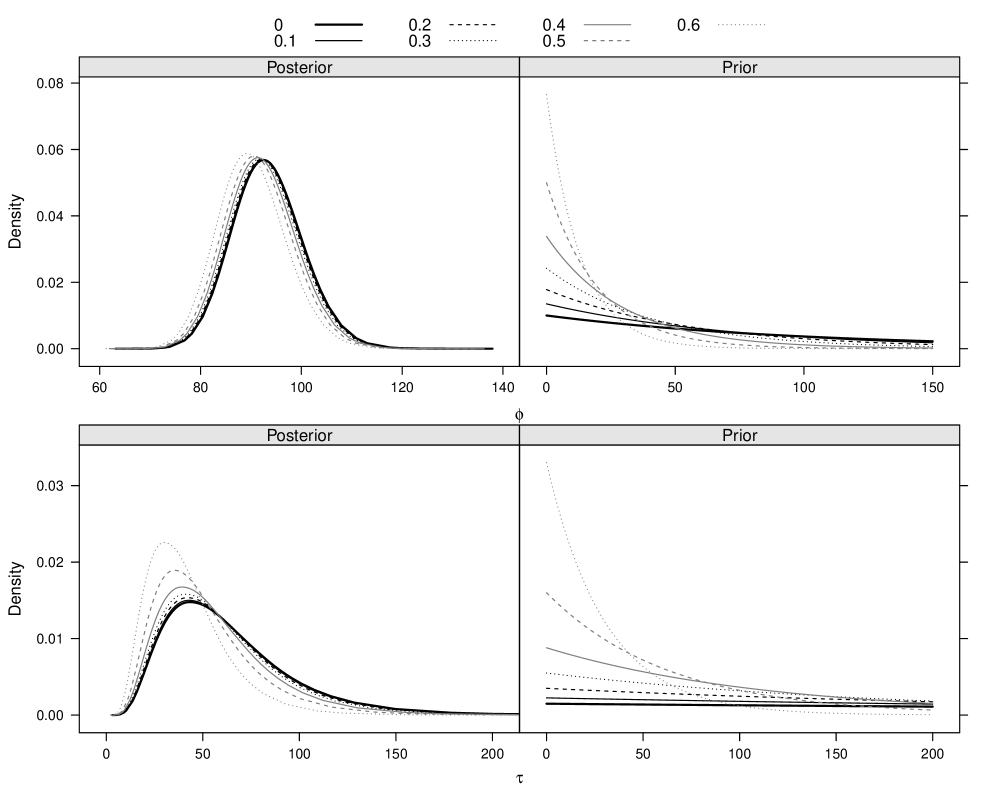
Figure 3: Posterior (left) and prior (right) distributions with Hellinger distances to the default prior ranging from 0.1 to 0.6 for the parameters $\phi$ (top) and $\tau$ (bottom).

Table 4 compare summary results of models with default prior default and with the largest Hellinger distance from the default prior. For $\phi$ the posterior mean changed from $93.37$ to $90.18$, a difference is only $3.53\%$ whereas for $\tau$ they change from $63.65$ to $41.86$ with a difference of $52.05\%$. Despite such differences, the practical conclusions on effects of relevance are unchanged since the changes are very small for the regression parameters. The relevance of the random effects in the model remains important.

Table 4: Summaries of the fitted models with Hellinger distances of 0.6 from the default prior for parameters $\phi$ and $\tau$.

	Default	Std. Err	$H(\phi_{D},\phi_{0.6})=0.6$	Std. Err	$H(\tau_{D},\tau_{0.6})=0.6$	Std. Err
$\beta_{0}$	0.3965	0.0520	0.3966	0.0518	0.3950	0.0607
$\beta_{1}$	-0.0724	0.0282	-0.0725	0.0287	-0.0719	0.0282
$\beta_{2}$	-0.1327	0.0299	-0.1327	0.0304	-0.1320	0.0299
$\beta_{3}$	0.4700	0.0396	0.4695	0.0403	0.4718	0.0396
$\phi$	93.3746	7.0019	90.1881	6.7830	93.5137	6.9848
$\tau_{1}^{2}$	63.6521	34.2202	64.8726	34.3975	41.8625	20.8770

5 Conclusion

This paper reports results of a Bayesian analysis of beta mixed models comparing results obtained with the INLA method with the ones obtained with an MCMC algorithm and purely likelihood analysis. Emphasis is placed on the specification and sensitivity of priors for the Beta dispersion parameter and the precision of the random effects.

Results of the analysis of the index of life quality for the worker’s on the Brazilian industrial sector indicates company size and average income are both relevant for the quality of life, as well as the effect of the states captured by adding a random intercept to the regression model. The analysis consisted of fitting several models with one final model chosen according to three criteria of model comparisons – LML, DIC and CPO. All criteria points to the same model choice. Summary results obtained with INLA are similar with the ones obtained with MCMC and likelihood analysis showing the substantial gain in the computational burden makes INLA an attractive choice for inference which allowing for several modeling alternatives to be investigated.

The sensitivity analysis was conducted for the dispersion parameters in the Bayesian beta mixed model using the Hellinger divergence as a measure of the distance between prior and posterior distributions. Our results show that the Beta dispersion parameter $\phi$ is insensitive to the choice of prior. Slightly more sensitive is the parameter $\tau$ related to the random effects, but the overall results and conclusions remains unchanged for the alternative priors.

- (1)
- Belitz et al. (2012) Belitz, C., Brezger, A., Kneib, T., Lang, S. and Umlauf, N. (2012). BayesX: Software for Bayesian Inference in Structured Additive Regression Models. Version 2.1.
- Bonat et al. (2012) Bonat, W. H., Ribeiro Jr, P. J. and Zeviani, W. M. (2012). Regression models with response on the unity interval: Specification, estimation and comparison., Biometric Brazilian Journal 30(4): 415–431.
- Bonat et al. (2013) Bonat, W. H., Ribeiro, Jr., P. J. and Zeviani, W. M. (2013). Likelihood analysis for a class of beta mixed models, ArXiv e-prints .
- Branscum et al. (2007) Branscum, A. J., Johnson, W. O. and Thurmond, M. C. (2007). Bayesian beta regression: applications to household expenditure data and genetic distance between foot-and-mouth disease viruses, Australian & New Zealand Journal of Statistics 49(3): 287–301.
- Breslow and Clayton (1993) Breslow, N. E. and Clayton, D. G. (1993). Approximate inference in generalized linear mixed models, Journal of the American Statistical Association 88(421): 9–25.
- Cepeda (2001) Cepeda, E. (2001). Variability Modeling in Generalized Linear Models, PhD thesis, Mathematics Institute, Universidade Federal do Rio de Janeiro.
- Cepeda and Gamerman (2005) Cepeda, E. and Gamerman, D. (2005). Bayesian methodology for modeling parameters in the two parameter exponential family, Estadística 57(1): 93–105.
- Chen et al. (2002) Chen, J., Zhang, D. and Davidian, M. (2002). A monte carlo em algorithm for generalized linear mixed models with flexible random effects distribution, Biostatistics 3(3): 347–360.
- Cribari-Neto and Zeileis (2010) Cribari-Neto, F. and Zeileis, A. (2010). Beta regression in R, Journal of Statistical Software 34(2): 1–24.
- da Silva et al. (2011) da Silva, C., Migon, H. and Correia, L. (2011). Dynamic Bayesian beta models, Computational Statistics & Data Analysis 55(6): 2074–2089.
- Espinheira et al. (2008a) Espinheira, P. L., Ferrari, S. L. and Cribari-Neto, F. (2008a). Influence diagnostics in beta regression, Computational Statistics & Data Analysis 52(9): 4417–4431.
- Espinheira et al. (2008b) Espinheira, P. L., Ferrari, S. L. and Cribari-Neto, F. (2008b). On beta regression residuals, Journal of Applied Statistics 35(4): 407–419.
- Ferrari and Cribari-Neto (2004) Ferrari, S. and Cribari-Neto, F. (2004). Beta regression for modelling rates and proportions, Journal of Applied Statistics 31(7): 799–815.
- Figueroa-Zúñiga et al. (2013) Figueroa-Zúñiga, J. I., Arellano-Valle, R. B. and Ferrari, S. L. (2013). Mixed beta regression: A Bayesian perspective, Computational Statistics & Data Analysis 61(0): 137–147.
- Fong et al. (2010) Fong, Y., Rue, H. and Wakefield, J. (2010). Bayesian inference for generalized linear mixed models, Biostatistics 11(3): 397–412.
- Grün et al. (2012) Grün, B., Kosmidis, I. and Zeileis, A. (2012). Extended beta regression in R: shaken, stirred, mixed, and partitioned, Journal of Statistical Software 48(11): 1–25.
- Grunwald et al. (1993) Grunwald, G. K., Raftery, A. E. and Guttorp, P. (1993). Time series of continuous proportions, Journal of the Royal Statistical Society, Series B 55(1): 103–116.
- Kieschnick and McCullough (2003) Kieschnick, R. and McCullough, B. D. (2003). Regression analysis of variates observed on (0, 1): percentages, proportions and fractions, Statistical Modelling 3(3): 193–213.
- Lele et al. (2010) Lele, S. R., Nadeem, K. and Schmuland, B. (2010). Estimability and likelihood inference for generalized linear mixed models using data cloning, Journal of the American Statistical Association 105(492): 1617–1625.
- Lunn et al. (2000) Lunn, D. J., Thomas, A., Best, N. and Spiegelhalter, D. (2000). Winbugs: A bayesian modelling framework: Concepts, structure, and extensibility, Statistics and Computing 10(4): 325–337.
- McKenzie (1985) McKenzie, E. (1985). An autoregressive process for beta random variables, Management Science 31(8): 988–997.
- Molenberghs and Verbeke (2005) Molenberghs, G. and Verbeke, G. (2005). Models for Discrete Longitudinal Data, Springer, New York.
- Nelder and Wedderburn (1972) Nelder, J. A. and Wedderburn, R. W. M. (1972). Generalized linear models, Journal of the Royal Statistical Society, Series A 135(3): 370–384.
- Ospina et al. (2006) Ospina, R., Cribari-Neto, F. and Vasconcellos, K. L. (2006). Improved point and interval estimation for a beta regression model, Computational Statistics & Data Analysis 51(2): 960–981.
- Ospina et al. (2011) Ospina, R., Cribari-Neto, F. and Vasconcellos, K. L. P. (2011). Erratum to "Improved point and interval estimation for a beta regression model" [Comput. statist. data anal. 51 (2006) 960-981], Computational Statatistics & Data Analysis 55(7): 2445.
- Paolino (2001) Paolino, P. (2001). Maximum likelihood estimation of models with beta-distributed dependent variables, Political Analysis 9(4): 325–346.
- Pinheiro and Bates (2000) Pinheiro, J. C. and Bates, D. M. (2000). Mixed-Effects Models in S and S-Plus, Springer. ISBN 0-387-98957-0.
- Plummer (2003) Plummer, M. (2003). JAGS: a program for analysis of Bayesian graphical models using Gibbs sampling, Proceedings of the 3rd International Workshop on Distributed Statistical Computing.
- R Development Core Team (2012) R Development Core Team (2012). R: A Language and Environment for Statistical Computing, R Foundation for Statistical Computing, Vienna, Austria. ISBN 3-900051-07-0.
- Rocha and Simas (2011) Rocha, A. and Simas, A. (2011). Influence diagnostics in a general class of beta regression models, TEST 20(1): 95–119.
- Rocha and Cribari-Neto (2008) Rocha, A. V. and Cribari-Neto, F. (2008). Beta autoregressive moving average models, Test 18(3): 529–545.
- Roos and Held (2011) Roos, M. and Held, L. (2011). Sensitivity analysis in bayesian generalized linear mixed models for binary data, Bayesian Analysis 6(2): 259–278.
- Rue et al. (2009) Rue, H., Martino, S. and Chopin, N. (2009). Approximate Bayesian inference for latent Gaussian models by using integrated nested Laplace approximations, Journal of the Royal Statistical Society, Series B 71(2): 319–392.
- Rue et al. (2013 +0100) Rue, H., Martino, S., Lindgren, F., Simpson, D. and Riebler, A. (2013 +0100)). INLA: Functions which allow to perform full Bayesian analysis of latent Gaussian models using Integrated Nested Laplace Approximaxion. R package version 0.0-1386148697.
- Simas et al. (2010) Simas, A. B., Barreto-Souza, W. and Rocha, A. V. (2010). Improved estimators for a general class of beta regression models, Computational Statistics & Data Analysis 54(2): 348–366.
- Smithson and Verkuilen (2006) Smithson, M. and Verkuilen, J. (2006). A better lemon squeezer? Maximum-likelihood regression with beta-distributed dependent variables, Psychological Methods 11(1): 54–71.
- Verkuilen and Smithson (2012) Verkuilen, J. and Smithson, M. (2012). Mixed and mixture regression models for continuous bounded responses using the beta distribution, Journal of Educational and Behavioral Statistics 37(1): 82–113.
- Wakefield (2009) Wakefield, J. (2009). Multi-level modelling, the ecologic fallacy, and hybrid study designs, International Journal of Epidemiology 38(2): 330–336.