Reaching NNLOPS accuracy with POWHEG and MiNLO

Abstract

We describe how a simulation of Higgs boson production accurate at next-to-next-to-leading order and matched to a parton shower can be built by combining the POWHEG and MiNLO methods and using Hnnlo results as input.

1 Introduction

During the last decade a major research effort in the Monte Carlo community has been devoted to the development of NLOPS tools, i.e. tools that allow a matching of next-to-leading order (NLO) computations with parton showers (PS), thereby bringing NLO accuracy into standard Monte Carlo event generators [1]. Among many proposals, there are currently two well-established NLOPS approaches, namely POWHEG [2, 3] and MC@NLO [4], which have now become the methods of choice used by experimental collaborations in many searches being carried out at the LHC. Part of this success was possible due to the progress in the automation of NLO computations, in the development of semiautomated or fully-automated NLOPS frameworks [5, 6, 7, 8], as well as in the standardization of well-defined interfaces [9, 10] between programs that operate different tasks.

A topic of research that has received much attention during the last 2 years is the merging of multiple NLOPS simulations for different jet multiplicities. These advances represent the NLO generalization of well-established tree-level multileg merging approaches [11, 12], and their relevance for future LHC phenomenology is clear, since they will allow a significant improvement in the simulation of processes where a heavy system is produced in association with multiple jets, which is the generic background for many new-Physics searches. There have been several proposals aiming at this goal [13, 14, 15, 16, 17, 18, 19, 20], among which the MiNLO approach [21, 19].

After a short review of the POWHEG and MiNLO approaches, I will describe how their combination can be used to match NNLO computations with PS, and show recent results obtained for inclusive Higgs production [22].

1.1 POWHEG

The POWHEG method is a prescription to interface NLO calculations with parton shower generators avoiding double counting of real emissions and virtual corrections. In the POWHEG formalism, the generation of the hardest emission is performed first, according to the distribution given by

$$d\sigma=\bar{B}\left(\Phi_{B}\right)\,d\Phi_{B}\,\left[\Delta_{R}\left(p_{T}^{\min}\right)+\frac{R\left(\Phi_{R}\right)}{B\left(\Phi_{B}\right)}\,\Delta_{R}\left(k_{T}\left(\Phi_{R}\right)\right)\,d\Phi_{\mathrm{rad}}\right]\,,$$ (1)

where $B\left(\Phi_{B}\right)$ is the leading order contribution,

$$\bar{B}\left(\Phi_{B}\right)=B\left(\Phi_{B}\right)+\left[V\left(\Phi_{B}\right)+\int d\Phi_{\mathrm{rad}}\,R\left(\Phi_{R}\right)\right]$$ (2)

is the NLO differential cross section integrated on the radiation variables while keeping the Born kinematics fixed ($V\left(\Phi_{B}\right)$ and $R\left(\Phi_{R}\right)$ stand respectively for the virtual and the real corrections), and $\Delta_{R}\left(p_{T}\right)=\exp\left[-\int d\Phi_{\mathrm{rad}}\,\frac{R\left(\Phi_{R}\right)}{B\left(\Phi_{B}\right)}\,\theta\left(k_{T}\left(\Phi_{R}\right)-p_{T}\right)\right]\,$ is the POWHEG Sudakov. With $k_{T}\left(\Phi_{R}\right)$ we denote the transverse momentum of the emitted particle off a Born-like kinematics $\Phi_{B}$, and, as usual, the cancellation of soft and collinear singularities is understood in the expression within the square bracket in eq. (2). Partonic events with hardest emission generated according to eq. (1) are then showered with a $k_{T}$-veto on following emissions. Subject to these conditions, it can be shown that such events exhibit the features typical of PS when the chosen observable probes the soft-collinear regions (Sudakov suppression), reproduce the exact fixed-order results in the regions where emissions are widely separated, and, crucially, they preserve NLO accuracy for inclusive observables. From the NLOPS-matching point of view, the more challenging processes currently described with this approach are $2\to 3$ and $2\to 4$ processes, with at most 2 light jets at LO [23, 24, 25, 26].

For the benefit of the following discussion, the (unregulated) $\bar{B}$ function of the standard POWHEG simulation of $H+1$ jet can be written schematically as

$$\bar{B}_{\,\tt HJ}=\alpha_{\scriptscriptstyle\rm S}^{3}(\mu_{R})\Big{[}B+\alpha_{\scriptscriptstyle\rm S}V(\mu_{R})+\alpha_{\scriptscriptstyle\rm S}\int d\Phi_{\mathrm{rad}}R\Big{]}\,,$$ (3)

where we have made explicit the dependence of all terms upon $\alpha_{\scriptscriptstyle\rm S}$ and the renormalization scale $\mu_{R}$. It is also worth recalling that when one or more jets are present at LO (as in the $H+1$ jet case) the associated $\bar{B}$ function needs to be regulated from the divergences arising when jets in the LO kinematics become unresolved [27]: as a consequence, a standard POWHEG simulation of $H+1$ jet cannot be used to describe inclusive Higgs production.

1.2 MiNLO

It is known that a common issue present in multileg NLO computations is the choice of the factorization ($\mu_{F}$) and renormalization scale: ultimately the problem is due to the fact that these computations are characterized by kinematical regimes involving several different scales, and, although some choices are clearly pathologic (as they can lead for instance to negative cross sections), in general there is no procedure to a-priori choose $\mu_{R}$ and $\mu_{F}$, being the scale dependence of the result just an artefact of truncating the perturbative expansion.

The MiNLO procedure [21] was originally defined as a prescription to address this issue, and it works by consistently including CKKW-like corrections into a standard NLO computation. By clustering with a $k_{T}$-measure the momenta of each phase-space point occurring in the computation, one can define the “most-probable” branching history that would have produced such a kinematics: the argument of each power of $\alpha_{\scriptscriptstyle\rm S}$ is then found from the transverse momentum of the splitting occurring at each nodal point of the skeleton built from clustering, and a prescription for $\mu_{F}$ is given as well. The result is also corrected by means of Sudakov form factors (called MiNLO-Sudakov FF’s in the following) associated to internal lines, accounting for the large logarithms that arise when the clustered event contains well separated scales.

Because of the presence of MiNLO-Sudakov FF’s associated to the Born-like kinematics, the integration over the full phase space $\Phi_{B}$ can be performed without generation cuts: a MiNLO-improved computation yields finite results also when jets in the LO kinematics become unresolved. As a consequence, the MiNLO procedure can be used within the POWHEG formalism to regulate the $\bar{B}$ function for processes involving jets at LO, without using external cuts or variants thereof.

MiNLO-enhanced POWHEG simulations have been presented in refs. [21, 19, 28, 29] and, in particular, in the $H+1$ jet case, the master formula for generating the hardest emission contains the following $\bar{B}$ function

$$\bar{B}_{\,\tt HJ-MiNLO} = \alpha_{\scriptscriptstyle\rm S}^{2}(M_{H})\alpha_{\scriptscriptstyle\rm S}(q_{T})\Delta^{2}_{g}(q_{T},M_{H})$$

$$\times \Big{[}B(1-2\Delta^{(1)}_{g}(q_{T},M_{H}))+\alpha_{\scriptscriptstyle\rm S}V(\bar{\mu}_{R})+\alpha_{\scriptscriptstyle\rm S}\int d\Phi_{\mathrm{rad}}R\Big{]}\,,$$

that should be contrasted with eq. (3). In eq. (1.2) $q_{T}$ is the Higgs transverse momentum (in the underlying-Born kinematics), $M_{H}$ is its virtuality, $\bar{\mu}_{R}$ is set to $(M_{H}^{2}q_{T})^{1/3}$ in accordance with the MiNLO prescription and $\Delta_{g}(q_{T},Q)=\exp\Big{\{}-\int_{q^{2}_{T}}^{Q^{2}}\frac{dq^{2}}{q^{2}}\frac{\alpha_{\scriptscriptstyle\rm S}(q^{2})}{2\pi}\Big{[}A_{g}\log\frac{Q^{2}}{q^{2}}+B_{g}\Big{]}\Big{\}}$ is the MiNLO-Sudakov FF associated to the jet present at LO. At NLL, the $A_{1,g}$, $A_{2,g}$ and $B_{1,g}$ terms in the expansion of $A_{g}$ and $B_{g}$ need to be included [21]. The term in brackets multiplying $B$ is needed to avoid double-counting of NLO factors: $\Delta_{g}^{(1)}(q_{T},Q)=-\frac{\alpha_{\scriptscriptstyle\rm S}}{2\pi}\Big{[}\frac{1}{2}A_{1,g}\log^{2}\frac{Q^{2}}{q_{T}^{2}}+B_{1,g}\log\frac{Q^{2}}{q_{T}^{2}}\Big{]}$ corresponds to the $\mathcal{O}(\alpha_{\scriptscriptstyle\rm S})$ expansion of $\Delta_{g}$.

The $\bar{B}$ function in eq. (1.2) can be integrated over the full phase space associated with the “LO” jet, yielding a finite cross-section for inclusive Higgs production. The formal accuracy of the result so obtained was carefully addressed in ref. [19], by means of a comparison with the NNLL $q_{T}$-resummation of the Higgs transverse momentum. It was found that, in order to reach NLO accuracy for the total inclusive Higgs production, the NNLL $B_{2,g}$ term should be included in the MiNLO-Sudakov FF, and $q_{T}$ should be used as factorization scale and as the argument of the power of $\alpha_{\scriptscriptstyle\rm S}$ associated to $R$, $V$ and $\Delta_{g}^{(1)}$ (i.e. the power of $\alpha_{\scriptscriptstyle\rm S}$ where no argument was specified in eq. (1.2)). If such terms are not included properly, spurious terms of order $\alpha_{\scriptscriptstyle\rm S}^{3.5}$ are generated upon integration over the entire Higgs $p_{T}$ spectrum, violating the requirement $[d\sigma_{\tt HJ-MiNLO}]_{\rm integrated}-\sigma_{\rm NLO}(gg\to H)=\mathcal{O}(\alpha_{\scriptscriptstyle\rm S}^{4})$, which is needed to claim NLO accuracy for fully-inclusive Higgs production.

2 Higgs production with NNLOPS accuracy

The $H+1$ jet POWHEG implementation enhanced with the improved MiNLO procedure previously outlined can be used to reach NNLOPS accuracy. In fact, since such a simulation gives a NLO-accurate prediction of the Higgs rapidity ($y$), then the function $W(y)$, defined as

$$W(y)=\frac{(d\sigma/dy)_{\rm NNLO}}{(d\sigma/dy)_{\tt HJ-MiNLO}}\,,$$ (5)

can be used to reweight each HJ-MiNLO-generated event, thereby obtaining a NNLOPS simulation of inclusive Higgs production. By NNLOPS we mean a fully-exclusive Monte Carlo simulation of Higgs-production which is NNLO accurate when one is fully inclusive on extra radiation, as well as LO (NLO) accurate for $H+2(1)$ jet observables [19, 22]. Since we are reweighting with $W$, the Higgs rapidity is NNLO accurate by construction, whereas the NLO accuracy of the 1-jet region, inherited from the underlying HJ-MiNLO simulation, is not spoiled, because the first non-controlled terms in the whole simulation are $\mathcal{O}(\alpha_{\scriptscriptstyle\rm S}^{5})$: this follows from the fact that $W(y)=1+\mathcal{O}(\alpha_{\scriptscriptstyle\rm S}^{2})$, as can be seen expanding numerator and denominator in eq. (5).

In ref. [22] the following generalization of eq. (5) was used:

$$W(y,p_{T})=h(p_{T})\frac{\int d\sigma_{\rm NNLO}\delta(y-y(\Phi))-\int d\sigma_{\tt HJ-MiNLO}^{B}\delta(y-y(\Phi))}{\int d\sigma_{\tt HJ-MiNLO}^{A}\delta(y-y(\Phi))}+(1-h(p_{T}))\,,$$ (6)

where we have split the HJ-MiNLO differential cross section among $d\sigma^{A}=d\sigma\ h(p_{T})$ and $d\sigma^{B}=d\sigma\ (1-h(p_{T}))$, with $h(p_{T})=\frac{(\beta m_{H})^{2}}{(\beta m_{H})^{2}+p_{T}^{2}}$. The profiling function $h$ controls where the NLO-to-NNLO correction is spread: as $2^{\mbox{\scriptsize{nd}}}$ argument of $W$ the transverse momentum of the leading jet was used, and we have chosen $\beta=1/2$, which implies that the NNLO correcting factor $W$ is effectively applied in the region $p_{T}\lesssim m_{H}/2$ (for $p_{T}\gg m_{H}$, $W(y,p_{T})\to 1$). With the choice in eq. (6) one also has that $(d\sigma/dy)_{\rm NNLOPS}$ reproduces $(d\sigma/dy)_{\rm NNLO}$ exactly, without $\mathcal{O}(\alpha_{\scriptscriptstyle\rm S}^{5})$ ambiguities.

2.1 Results

In our simulation, the central value for $d\sigma_{\rm NNLO}$ was obtained with Hnnlo [30, 31], setting $\mu_{R}=\mu_{F}=m_{H}/2$. We refer to ref. [22] for details on how scales were varied to obtain uncertainty bands.

In fig. 1 a comparison between our NNLOPS simulation and Hnnlo is shown: as expected, the NNLOPS simulation reproduces extremely well the NNLO results for the Higgs rapidity both in the central value and in the uncertainty band obtained by scale variation.

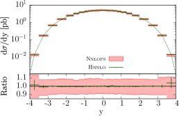
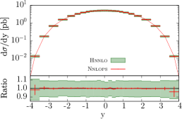
Figure 1: Comparison of the NNLOPS (red) and Hnnlo (green) results for the Higgs fully inclusive rapidity distribution. On the left (right) plot only the NNLOPS (Hnnlo) uncertainty is displayed. The lower left (right) panel shows the ratio with respect to the NNLOPS (Hnnlo) prediction obtained with its central scale choice.

Fig. 2 shows the Higgs transverse momentum $p_{T}^{H}$. We compare our simulation with HqT [32, 33], whose central value is obtained with $Q_{\rm res}=m_{H}/2$ and $\mu_{R}=\mu_{F}=m_{H}/2$. The HqT result corresponds to a NNLL prediction of $p_{T}^{H}$, matched to the fully inclusive cross section at NNLO. Here we notice that the two results are almost completely contained within each other’s uncertainty band in the region of low-to-moderate transverse momenta. The central values at small momenta also exhibit a very good agreement, supporting our choice for $\beta$. The difference in the large-$p_{T}$ tail is not a reason of concern, and it is expected since the two predictions use different scales at large $p_{T}$, as explained in ref. [22].

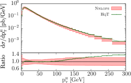
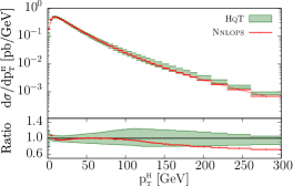
Figure 2: Comparison of the NNLOPS (red) with the NNLL+NNLO prediction of HqT (green) for the Higgs transverse momentum. In HqT we keep the resummation scale $Q_{\rm res}$ always fixed to $m_{H}/2$ and vary $\mu_{R}$ and $\mu_{F}$. On the left (right), the NNLOPS (HqT) uncertainty band is shown. In the lower panel, the ratio to the NNLOPS (HqT) central prediction is displayed.

Finally, we also mention that a comparison among NNLOPS and NNLL+NNLO predictions from JetVHeto [34] was successfully carried out for the jet veto efficiency, defined as the cross section for Higgs boson production events containing no jets with transverse momentum greater than a given value ($p_{\scriptscriptstyle\mathrm{T,veto}}$), divided by the respective total inclusive cross section. The central predictions of the two programs are never out of agreement by more than 5-6%, and the two sets of predictions lie within each other’s error bands essentially everywhere over all values of $p_{\scriptscriptstyle\mathrm{T,veto}}$, as shown in ref. [22].

- [1] A. Buckley, J. Butterworth, S. Gieseke, D. Grellscheid, S. Hoche, H. Hoeth, F. Krauss and L. Lonnblad et al., Phys. Rept. 504, 145 (2011) [arXiv:1101.2599 [hep-ph]].
- [2] P. Nason, JHEP 0411, 040 (2004) [hep-ph/0409146].
- [3] S. Frixione, P. Nason and C. Oleari, JHEP 0711, 070 (2007) [arXiv:0709.2092 [hep-ph]].
- [4] S. Frixione and B. R. Webber, JHEP 0206, 029 (2002) [hep-ph/0204244].
- [5] S. Alioli, P. Nason, C. Oleari and E. Re, JHEP 1006, 043 (2010) [arXiv:1002.2581 [hep-ph]].
- [6] R. Frederix, S. Frixione, V. Hirschi, F. Maltoni, R. Pittau and P. Torrielli, Phys. Lett. B 701, 427 (2011) [arXiv:1104.5613 [hep-ph]].
- [7] S. Platzer and S. Gieseke, Eur. Phys. J. C 72, 2187 (2012) [arXiv:1109.6256 [hep-ph]].
- [8] S. Hoeche, F. Krauss, M. Schonherr and F. Siegert, JHEP 1209, 049 (2012) [arXiv:1111.1220 [hep-ph]].
- [9] T. Binoth, F. Boudjema, G. Dissertori, A. Lazopoulos, A. Denner, S. Dittmaier, R. Frederix and N. Greiner et al., Comput. Phys. Commun. 181, 1612 (2010) [arXiv:1001.1307 [hep-ph]].
- [10] S. Alioli, S. Badger, J. Bellm, B. Biedermann, F. Boudjema, G. Cullen, A. Denner and H. van Deurzen et al., arXiv:1308.3462 [hep-ph].
- [11] S. Catani, F. Krauss, R. Kuhn and B. R. Webber, JHEP 0111, 063 (2001) [hep-ph/0109231].
- [12] M. L. Mangano, M. Moretti, F. Piccinini and M. Treccani, JHEP 0701, 013 (2007) [hep-ph/0611129].
- [13] S. Alioli, K. Hamilton and E. Re, JHEP 1109, 104 (2011) [arXiv:1108.0909 [hep-ph]].
- [14] S. Hoeche, F. Krauss, M. Schonherr and F. Siegert, JHEP 1304, 027 (2013) [arXiv:1207.5030 [hep-ph]].
- [15] R. Frederix and S. Frixione, JHEP 1212, 061 (2012) [arXiv:1209.6215 [hep-ph]].
- [16] S. Platzer, JHEP 1308, 114 (2013) [arXiv:1211.5467 [hep-ph]].
- [17] S. Alioli, C. W. Bauer, C. J. Berggren, A. Hornig, F. J. Tackmann, C. K. Vermilion, J. R. Walsh and S. Zuberi, JHEP 1309, 120 (2013) [arXiv:1211.7049 [hep-ph]].
- [18] L. Lonnblad and S. Prestel, JHEP 1303, 166 (2013) [arXiv:1211.7278 [hep-ph]].
- [19] K. Hamilton, P. Nason, C. Oleari and G. Zanderighi, JHEP 1305, 082 (2013) [arXiv:1212.4504].
- [20] L. Hartgring, E. Laenen and P. Skands, JHEP 1310, 127 (2013) [arXiv:1303.4974 [hep-ph]].
- [21] K. Hamilton, P. Nason and G. Zanderighi, JHEP 1210, 155 (2012) [arXiv:1206.3572 [hep-ph]].
- [22] K. Hamilton, P. Nason, E. Re and G. Zanderighi, JHEP 1310, 222 (2013) [arXiv:1309.0017 [hep-ph]].
- [23] J. M. Campbell, R. K. Ellis, R. Frederix, P. Nason, C. Oleari and C. Williams, JHEP 1207, 092 (2012) [arXiv:1202.5475 [hep-ph]].
- [24] E. Re, JHEP 1210, 031 (2012) [arXiv:1204.5433 [hep-ph]].
- [25] B. Jager, S. Schneider and G. Zanderighi, JHEP 1209, 083 (2012) [arXiv:1207.2626 [hep-ph]].
- [26] B. Jager and G. Zanderighi, JHEP 1304, 024 (2013) [arXiv:1301.1695 [hep-ph]].
- [27] S. Alioli, P. Nason, C. Oleari and E. Re, JHEP 1101, 095 (2011) [arXiv:1009.5594 [hep-ph]].
- [28] J. M. Campbell, R. K. Ellis, P. Nason and G. Zanderighi, JHEP 1308, 005 (2013) [arXiv:1303.5447 [hep-ph]].
- [29] G. Luisoni, P. Nason, C. Oleari and F. Tramontano, JHEP 1310, 083 (2013) [arXiv:1306.2542 [hep-ph]].
- [30] S. Catani and M. Grazzini, Phys. Rev. Lett. 98, 222002 (2007) [hep-ph/0703012].
- [31] M. Grazzini, JHEP 0802, 043 (2008) [arXiv:0801.3232 [hep-ph]].
- [32] G. Bozzi, S. Catani, D. de Florian and M. Grazzini, Nucl. Phys. B 737, 73 (2006) [hep-ph/0508068].
- [33] D. de Florian, G. Ferrera, M. Grazzini and D. Tommasini, JHEP 1111, 064 (2011) [arXiv:1109.2109 [hep-ph]].
- [34] A. Banfi, P. F. Monni, G. P. Salam and G. Zanderighi, Phys. Rev. Lett. 109, 202001 (2012) [arXiv:1206.4998 [hep-ph]].