Determination of the maximum Global Quantum Discord via measurements of excitations in a cavity QED network

Abstract

Multipartite Quantum Correlations is one of the most relevant indicator of the quantumness of a system in many body systems. This remarkable feature is in general difficult to characterize and the known definitions are hard to measure. Besides the efforts dedicated to solve this problem, the question of which is the best approach remains open. In this work, we study the Global Quantum Discord ($GQD$) as a bipartite and multipartite measure. We also check the limits of this definitions and present an experimental scheme to determine the maximum of the $GQD$ via the measurements of the system‘s excitations, during the time evolution of the present system.

I Introduction

Quantum correlations has been a hot topic during the last years due to their powerful applications in quantum information and computational tasks nielsen ; caves . For bipartite states, different measures as Entanglement($E$) wootters1 and Quantum Discord($QD$) QD ; QD1 are already well understood. Although, some times for multipartite systems, there are correlations which are not detected by the previous measurements. Many attempts of extending the bipartite correlations to the multipartite case have been made wootters ; zambrini ; fanchini ; sarandy , but still questions remain about these generalizations. One of the first approach was the Tangle wootters , that is related with $E$, but is difficult to compute for mixed states. Next, in another endeavor, Global Quantum Discord($GQD$) was defined in Ref.sarandy . This new measurement of correlations is a straight extension from the bipartite to multipartite case, it is symmetric and obeys monogamy properties. These unique advantages suggest the $GQD$ as a resource for quantum information processing.

More recently, much attention has been paid to the application of $GQD$ and it’s connection with criticality sarandy ; campbell , as the detection of phase transitions phase_transition ; phase_transition2 . Nevertheless, some questions are open, for example: is it possible to measure the $GQD$ experimentally, or know when it reaches it’s maximum value? To answer this question, we first will study the distribution of excitations in the system, and see how this distribution can affect the $GQD$. We also propose a model, which is a cavity QED system, where the $GQD$ has not been studied yet.

Over the past decades, cavity QED systems have been extensively researched, and several advantages, theoretical and experimentally, are known about these systems experiment ; cavities ; victor . The development of experimental techniques for their manipulation with an unprecedented level of control, as well as performing measurements inside the cavity are desirable features when choosing our model.

This paper is organized as follows: in section II, we describe our system, the Hamiltonian and write a generalized master equation, where the Lindblad terms result from the coupling of each cavity to it’s own thermal reservoir at zero temperature. In section III, we give a brief outline of the Global Quantum Discord. In section IV, we present the main results of this paper, related to the applicability of $GQD$ and we discuss our ability to gain, experimentally, information about this magnitude. Finally, section V is devoted to the conclusions.

II The Model

We have three coupled cavities, as shown in Fig.(1), where each cavity interacts with a single atom and it’s own reservoir. We choose Rydberg atoms with principal quantum numbers $51$ and $50$, where the transition is at $51,1$ GHz. The atom cavity strength coupling($g$), corresponds to an interaction time of $1$ $\mu$s. The photon life time inside the cavity is $T_{cav}=1$ ms haroche1 ; haroche2 . The coupling between the cavities($J$) is about $10^{-2}g$. We scale the time in the figures with $\gamma=10^{5}$.

Figure 1: Three Coupled Cavity-Atom Systems.

The Hamiltonian of the system, in the basis of the dressed states(polaritonic) angelakis , is given by:

$$\mathit{H}=\sum_{i=1}^{3}(\omega_{i}-g_{i})|E\rangle_{i}\langle E|++\sum_{i=1}^{2}\frac{J_{i}}{2}(L_{i}^{\dagger}L_{i+1}+L_{i}^{-}L_{i+1}^{\dagger})$$ (1)

where $|E_{i}\rangle=\frac{1}{\sqrt{2}}(|1,g\rangle_{i}-|0,e\rangle_{i})$ and $|G_{i}\rangle=|0,g\rangle_{i}$ are the dressed states, corresponding to excited and ground state respectively. The other operators $\mathit{L^{\dagger}_{i}}=|E_{i}\rangle\langle G_{i}|$ and $\mathit{L^{-}_{i}}=|G_{i}\rangle\langle E_{i}|$ are to create or destroy those states. So we can consider polaritons as two-level systems. We just can have one photon, at most, because due to photon blockade, double or higher occupancy of the polaritonic states is prohibited blockade1 ; blockade2 .

The main source of dissipation originates from the leakage of the cavity photons due to imperfect reflectivity of the cavity mirrors. A second source of dissipation, corresponding to atomic spontaneous emission, will be neglected assuming long atomic lifetimes.

An approach to model the above mentioned losses, in the presence of single mode quantized cavity field, is using the microscopic master equation, which goes back to the ideas of Davies on how to describe the system-reservoir interactions in a Markovian master equation davies . For a three-cavity-system at zero temperature, the master equation is raul ; serafini :

$$\dot{\rho}(t)=-i\left[\mathit{H_{s}},\rho(t)\right]+\sum_{n=1}^{3}\sum_{\omega>0}^{\infty}\gamma_{n}(\omega)\left(\mathit{A_{n}}(\omega)\rho(t)\mathit{{A}^{\dagger}_{n}}(\omega)-\frac{1}{2}\left\{\mathit{{A}^{\dagger}_{n}}(\omega)\mathit{A_{n}}(\omega),\rho(t)\right\}\right)$$ (2)

where $\mathit{A_{n}}$ correspond to the Davies’s operators. The sum on $n$ is over all the dissipation channels and the decay rate $\gamma_{n}(\omega)$ is the Fourier transform of the correlation functions of the environment petruccione .

The $\mathit{A_{n}}$ operators are calculated as follows:

$$\mathit{A_{n}}(\omega_{\alpha\beta})=|\phi\rangle_{\alpha}\langle\phi|a_{n}|\phi\rangle_{\beta}\langle\phi|$$ (3)

III Global Quantum Discord

In the original proposal QD , $QD$ was defined as a mismatch between quantum analogs of classically equivalent expressions of the mutual information.

$$\mathit{QD}(\rho_{AB})=\mathit{I}(\rho_{AB})-\mathit{J}(\rho_{AB})$$ (4)

The mutual information $\mathit{I}(\rho_{AB})$ of two subsystem can be expressed as

$$\mathit{I}(\rho_{AB})=S(\rho_{A})-S(\rho_{A}|\rho_{B}),$$ (5)

where $S(\rho)=-Tr(\rho\log_{2}\rho)$ is the von Neumann entropy, and $S(\rho_{A}|\rho_{B})=S(\rho_{AB})-S(\rho_{B})$.

The classical correlation $\mathit{J}(\rho_{AB})$ is defined as the maximum information that one can obtain from $A$ by performing a measurement on $B$, and in general this definition is not symmetric:

$$\mathit{J}(\rho_{AB})=\max_{\{\Pi_{B}^{k}\}}[S(\rho_{A})-S(\rho_{AB}|\{\Pi_{B}^{k}\})],$$ (6)

where $\{\Pi_{B}^{k}\}$ is a complete set of projectors performed on subsystem $B$ and $S(\rho_{AB}|\{\Pi_{B}^{k}\})=\sum_{k}p_{k}S(\rho_{A}^{k})$. The reduced density operator $\rho^{k}$ associated with the measurement result $k$ is:

$$\rho^{k}=\dfrac{1}{p_{k}}(\mathit{I}\otimes\Pi_{B}^{k})\rho(\mathit{I}\otimes\Pi_{B}^{k})$$ (7)

with $\mathit{I}$ the identity operator.

Notice that $\mathit{I}(\rho_{AB})$ can be rewritten in terms of the relative entropy, $S(\rho\|\sigma)=Tr(\rho\log_{2}\rho-\rho\log_{2}\sigma)$, as:

$$\mathit{I}(\rho_{AB})=S(\rho_{AB}\|\rho_{A}\otimes\rho_{B})$$ (8)

Also, by symmetrizing the definition through the introduction of bilateral measurements, and after some algebra we get a new definition of $QD$, given by:

$$GQD(\rho_{AB})=\min_{\{\Pi_{A}^{j}\otimes\Pi_{B}^{k}\}}[S(\rho_{AB}\|\Phi_{AB}(\rho_{AB}))-S(\rho_{A}\|\Phi_{A}(\rho_{A}))-S(\rho_{B}\|\Phi_{B}(\rho_{B}))]$$ (9)

with $\Phi(\rho_{AB})=\sum_{j,k}(\Pi_{A}^{j}\otimes\Pi_{B}^{k})\rho_{AB}(\Pi_{A}^{j}\otimes\Pi_{B}^{k})$. From Eq.(9) the generalization to multipartite discord is evident,

$$GQD(\rho_{A_{1}...A_{N}})=\min_{\{\Pi^{k}\}}[S(\rho_{A_{1}...A_{N}}\|\Phi(\rho_{A_{1}...A_{N}}))-\sum_{j=1}^{N}S(\rho_{A_{j}}\|\Phi(\rho_{A_{j}}))]$$ (10)

where $\Phi(\rho_{A_{j}})=\sum_{k}\Pi_{A_{j}}^{k}\rho_{A_{j}}\Pi_{A_{j}}^{k}$ and $\Phi(\rho_{A_{1}...A_{N}})=\sum_{k}\Pi_{k}\rho_{A_{1}...A_{N}}\Pi_{k}$, with $\Pi_{k}=\Pi_{A_{1}}^{k_{1}}\otimes\dots\otimes\Pi_{A_{N}}^{k_{N}}$ and $k$ denoting the index string $(j_{1}...j_{N})$.

IV Results

Genuine Tripartite Measure

It has been shown that $GQD$ is a multipartite measurement sarandy ; campbell , that not only measures tripartite quantum correlations, as the Tangle defined by Wootters wootters , but also bipartite correlations. This statement can be illustrated with the following example. If we prepare our system initially in a mixture of a genuine tripartite correlated state(GHZ) and a bipartite Bell state,

$$\rho(0)=\frac{\alpha}{2}(|EEE\rangle\langle EEE|+|GGG\rangle\langle GGG|)+\frac{(1-\alpha)}{2}(|\Psi\rangle\langle\Psi|\otimes|G\rangle_{2}\langle G|)$$ (11)

with $|\Psi\rangle=(|E_{1}G_{3}\rangle+|G_{1}E_{3}\rangle)$, as $\alpha$ increases from zero to one, the system goes from bipartite to tripartite correlations, but $GQD=1$ for all $\alpha$. The question is, what happens when we eliminate all the bipartite quantum discord? In Fig.(2) we plot the function $MGQD=GQD_{123}-GQD_{12}-GQD_{13}-GQD_{23}$, for the same initial state in Eq.(11). Notice that for $\alpha=0$ there is no multipartite correlation and for $\alpha=1$ the $MGQD$ is one, as expected from a $GHZ$ state. Near to $\alpha=0.7$ the function has a point where the derivative does not exist, this is because of the change in the angles during the numerical minimization.

Figure 2: Genuine tripartite global quantum discord increases from zero to one when the initial state goes from Bell to $GHZ$ state.

At this point, it seems that there is no problem with the new definition of genuine multipartite correlation. However, when we check the time evolution for $MGQD$, particularly for $\alpha=0$, the function becomes negative at certain times, see Fig.(3). We also tried the Werner’s state, obtaining similar results. This negative behavior of $MGQD$ is enhanced when the initial condition is near a pure bipartite correlated state.

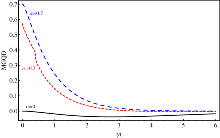
Figure 3: For $\alpha=0$ the $MGQD$ becomes negative, indicating that the $GQD$ does not include separately bipartite and tripartite correlations. $T_{cav}=10$ $\mu$s.

A first approach to solve this problem can be the use of the monogamy restrictions monogamy1 ; monogamy2 , where the exact solution is lost, but at least we can estimate a upper bound for the genuine tripartite correlations. From references monogamy1 and monogamy2 , we write two monogamy relations:

$$GQD(A:B:C)\geq GQD(A:B)+GQD(A:C)$$ (12)

$$GQD(A:B:C)\geq GQD(A:B)+GQD(B:C)$$ (13)

The authors of these two papers define a “Residual $GQD$”($D_{R}$) as the difference between the left hand and right hand side of above equations. The problem with the definition of $D_{R}$ is that is non symmetric with respect to the pairwise combinations. Instead, we define a new $D_{R}$, based on the above equations, getting:

$$GQD(A:B:C)\geq\frac{2}{3}(GQD(A:B)+GQD(B:C)+GQD(A:C))$$ (14)

In Fig.(4) we reported the comparison between $D_{R1}$, $D_{R2}$ and $D_{R3}$ from equations (12),(13) and (14) respectively. Already from the initial state there are differences among the three curves. Notice that the residual global discord corresponding to Eq.(12)(red-dotted), seems to be the most restrictive one. Nevertheless, that can be easily changed by starting with a bipartite correlation of cavities $2$ and $3$, instead cavities $1$ and $3$, which will change $D_{R2}$ to be the most restrictive one. But, our approach remains very well independent of the initial condition, as it includes all possible combination of pairwise correlations.

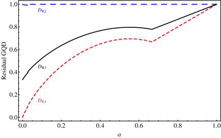
Figure 4: Residual $GQD$ corresponding to our definition($D_{R3}$) represents better the monogamy restriction, since it is a good approximation independently of the initial condition.

Next, we analyzed the time evolution of the above definitions for $\alpha=0.4$. In Fig.(5) we show that certainly $D_{R1}$ and our definition $D_{R3}$ are close. However, $D_{R1}$ is highly sensitive to initial conditions, which is not the case of $D_{R3}$, so we conclude that $D_{R3}$ is more suitable to describe the quantum correlations, for any initial condition.

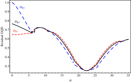
Figure 5: All definitions are close, during the time evolution of the system. We observe that $D_{R3}$ remains between the other two, again showing more stability to variations of the initial conditions.

Estimation of the $GQD$ by means of the excitation probabilitities of the subsystems

Quantum Correlation measurements are very important for quantum information and quantum computation, and even now is difficult to do it davidovich , especially for higher correlations as the tripartite one. However, there is a connection between the localization of the excitations throughout the system and the quantum correlations of it’s parts. To illustrate this, we first consider a typical bipartite Bell state $|\phi\rangle=\frac{1}{\sqrt{2}}(|10\rangle+|01\rangle)$. It is well known that this state is maximally correlated, but we also notice that the probability of finding an excitation in each subsystems is $1/2$. In other words, we could say in this example, that when the subsystems are highly correlated, the excitations are equally distributed through them.

In our system, things are more complicated, since we have three cavities and we could have up to three excitations. Nevertheless, the same rule applies. For example, let us assume that initially we have one excitation in cavity $2$, and let $P_{E1}$, $P_{E2}$ and $P_{E3}$ be the probabilities of finding the polariton in cavities $1$, $2$ and $3$ respectively. In Fig.(6), we plot the time evolution of $GQD$ and these three probabilities. We can readily see that when the three probabilities cross at a certain time, the $GQD$ reaches it’s maximum value, as in the case of two qubits. Thus we believe that the $GQD$ is associated with disorder or equal distribution of the excitations among the three cavities.

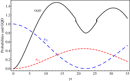
Figure 6: $GQD$ reaches it’s maximum when the three probabilities cross at certain time. Due to symmetry, $P_{E3}=P_{E1}$.

Similar results are also observed for the state in Eq.(11), see Fig.(7). Here we show the matrix’s elements of the density operator for $\alpha=0.1$ and $\alpha=0.5$. We used the standard basis: $|1\rangle=|EEE\rangle$,$|2\rangle=|EEG\rangle$,$|3\rangle=|EGE\rangle$,$|4\rangle=|GEE\rangle$,$|5\rangle=|EGG\rangle$,$|6\rangle=|GEG\rangle$,$|7\rangle=|GGE\rangle$,$|8\rangle=|GGG\rangle$. Each graphic corresponds to the maximum of the $GQD$. Notice that again the three probabilities, associated to the $|5\rangle\langle 5|$,$|6\rangle\langle 6|$ and $|7\rangle\langle 7|$ matrix elements, are equal.

The presence of the quantum correlations is related to the off diagonal elements of the density matrix. For long times, these elements as well as the correlations tend to disappear due to the losses.

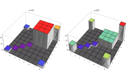
Figure 7: Density operator’s elements for the initial state in Eq(11). The maximum of $GQD$ is reached when $P_{E1}=P_{E2}=P_{E3}$ and the off-diagonal components do not vanish.

As we saw, one of the advantages of the $GQD$ is that for any mixed initial bipartite and tripartite state, with only one measurement we can estimate how correlated the subsystems are. Then, one could experimentally detect when the maximum $GQD$ is reached by measuring the polaritons in the cavities measure_polariton . To summarize, the $GQD$ can provides us valuable information about any class of multipartite correlations and furthermore, this can be experimentally observed by measuring the excitations of our system.

V Summary and Conclusions

We analized the Global Quantum Discord, as a measure of the joint bipartite and tripartite correlations. We showed it s limitations to detect a genuine tripartite correlation, since negative values show up. However, we presented an upper bound which turned out to be a good estimation, valid for any initial condition. Then we studied the relation between the disorder of the system and the $GQD$. Our goal was to associate the $GQD$ with some experimentally measurable quantity, such as the degree of excitation of each sub-system. We found that when excitations were nearly equally distributed, among the various sub-systems, the $GQD$ reached it s maximal value.

Moreover, the sensitivity of this measure, which is certainly related with the bilateral projection and the minimization process, seems very interesting for it’s different applications. In order to illustrate this feature, we focus on the sudden transition effect sudden_trans ; sudden_trans2 . This effect depends strongly on the the initial conditions, and it can be seen only when some restrictions are fulfilled. For example, we start with the initial state proposed in reference sudden_trans for the cavities $1$ and $3$, and assume for the second cavity to be in an excited or ground state.

$$\rho(0)=\begin{pmatrix}(1+c_{3})&0&0&(c_{1}-c_{2})\\ 0&(1-c_{3})&(c_{1}+c_{2})&0\\ 0&(c_{1}+c_{2})&(1-c_{3})&0\\ (c_{1}-c_{2})&0&0&(1+c_{3})\end{pmatrix}\otimes|\mathit{i}\rangle_{2}\langle\mathit{i}|$$ (15)

where the matrix is in the basis:$|EE\rangle$,$|EG\rangle$,$|GE\rangle$,$|GG\rangle$, and $|\mathit{i}\rangle=\left\{|E\rangle,|G\rangle\right\}$.

In Fig.(8) we plotted the quantum discord, defined in Eq.(9) between cavities $1$ and $3$, when cavity $2$ is initially in the state $|G\rangle$, and weakly coupled to the other two cavities. The parameters are: $c_{1}=1$,$c_{2}=-c_{3}$ and $c_{3}=0.8$. The inset corresponds to a zoom at the beginning of the curve. We observe rapid oscillations that have not been reported before, for this particular measure, and also abrupt changes in the derivative, which is quite unusual. We did the same for $QD$ defined in Eq.(4), following two different approaches alber ; caldeira , and we did not find such effects in neither case. This evidences that $GQD$, proposed in reference sarandy is more sensitive than the others.

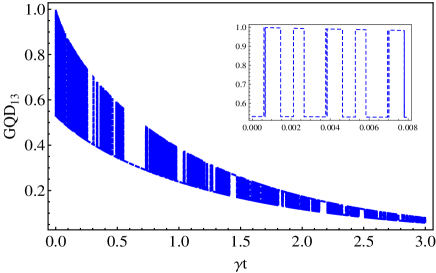
Figure 8: Sudden changes in the bipartite global quantum discord for the cavities $1,3$. $T_{cav}=10$ $\mu$s.

VI Acknowledgements

M. Orszag acknowledges financial support from Fondecyt, Project $1100039$ and Programa de Investigacion asociativa anillo ACT-1112. R. Coto thanks the support from the Pontificia Universidad Católica de Chile.

References

- (1) Nielsen M and Chuang I 2000 Quantum Information and Quantum Computation(Cambridge: Cambridge University Press)
- (2) Datta A, Shaji A, and Caves C M 2008 Phys. Rev. Lett. 100 050502
- (3) Wootters W K 1998 Phys. Rev. Lett. 80 2245
- (4) Ollivier H and Zurek W H 2002 Phys. Rev. Lett. 88 017901
- (5) The discord as a Bures distance, see: Spehner D and Orszag M 2013 New J. Phys. 15 103001; see also Spehner D and Orszag M, to appear in J. Phys.A; arXiv:1304.3334(quant-phys)
- (6) Coffman V, Kundu J and Wootters W K 2000 Phys. Rev. A 61 052306
- (7) Giorgi G L, Bellomo B, Galve F and Zambrini R 2011 Phys. Rev. Lett. 107 190501
- (8) ZhiHao Ma, ZhiHua Chen and Fanchini F F 2013 New J. Phys. 15 043023
- (9) Rulli C C and Sarandy M S 2011 Phys. Rev. A 84 042109
- (10) Campbell S, Mazzola L, De Chiara G, Apollaro T J G, Plastina F, Busch T and Paternostro M 2013 New J. Phys. 15 043033
- (11) Werlang T, Trippe C, Ribeiro G A P and Rigolin G 2010 Phys. Rev. Lett. 105 095702
- (12) Werlang T, Ribeiro G A P and Rigolin G 2011 Phys. Rev. A 83 062334
- (13) Ritter S, Nolleke C, Hahn C, Reiserer A, Neuzner A, Uphoff M, Mucke M, Figueroa E, Bochmann J and Rempe G 2012 Nature 484 195
- (14) Hartmann M J, Brandao F G S L and Plenio M B 2008 Laser Photon. Rev. 2 No.6 527556
- (15) Montenegro V, Orszag M 2011 J. Phys. B: At. Mol. Opt. Phys. 44 154019; for thermal effects, see also Eremeev V, Montenegro V and Orszag M 2012 Phys. Rev. A 85 032315
- (16) Raimond J M, Brune M and Haroche S 2001 Rev. Mod. Phys. 73 565
- (17) Brune M, Schmidt-Kaler F, Maali A, Dreyer J, Hagley E, Raimond J M and Haroche S 1996 Phys. Rev. Lett. 76 1800
- (18) Angelakis D G, Santos M F and Bose S 2007 Phys. Rev. A 76 031805(R)
- (19) Birnbaum K M, Boca A, Miller R, Boozer A D, Northup T E, and Kimble H J 2005 Nature 436 87
- (20) Imamoglu A, Schmidt H, Woods G and Deutsch M 1997 Phys. Rev. Lett. 79 1467
- (21) Davies E B 1976 Quantum theory of open system(London: Academic)
- (22) Coto R and Orszag M 2013 J. Phys. B: At. Mol. Opt. Phys. 46 175503
- (23) Serafini A, Mancini S and Bose S 2006 Phys. Rev. Lett. 96 010503
- (24) Breuer H and Petruccione F 2002 The Theory of Open Quantum Systems(Oxford: University Press)
- (25) Braga H C, Rulli C C, De Oliveira R and Sarandy M S 2012 Phys. Rev. A 86 062106
- (26) Si-Yuan Liu, Yu-Ran Zhang, Li-Ming Zhao, Wen-Li Yang and Heng Fan arXiv:11307.4848
- (27) Farias O J, Aguilar G H, Valdes-Hernandez A, Souto Ribeiro P H, Davidovich L and Walborn S P 2012 Phys. Rev. Lett. 109 150403
- (28) Toyoda K, Matsuno Y, Noguchi A, Haze S and Urabe S 2013 Phys. Rev. Lett. 111 160501
- (29) Mazzola L, Piilo J and Maniscalco S 2010 Phys. Rev. Lett. 104 200401
- (30) Qi-Liang He, Jing-Bo Xu, Dao-Xin Yao and Ye-Qui Zhang 2011 Phys. Rev. A 84 022312
- (31) Ali M, Rau A R P and Alber G 2010 Phys. Rev. A 81 042105
- (32) Fanchini F F, Werlang T, Brasil C A, Arruda L G E and Caldeira A O 2010 Phys. Rev. A 81 052107