Pseudo Slice Energy Spread
in Dynamics of Electron Beams Moving through Magnetic Bends

Abstract

In the previous canonical formulation of beam dynamics for an electron bunch moving ultrarelativistically through magnetic bending systems, we have shown that the transverse dynamics equation for a particle in the bunch has a driving term which behaves as the centrifugal force caused by the particle’s initial potential energy due to collective particle interactions within the bunch. As a result, the initial potential energy at the entrance of a bending system, which we call pseudo (kinetic) energy, is indistinguishable from the usual kinetic energy offset from the design energy in its perturbation to particle optics through dispersion and momentum compaction. In this paper, in identifying this centrifugal force on particles as the remnant of the CSR cancellation effect in transverse particle dynamics, we show how the dynamics equation in terms of the canonical momentum for beam motion on a curved orbit is related to the Panofsky-Wenzel theorem for wakefields for beam motion on a straight path. It is shown that the effect of pseudo energy spread can be measurable only for a high-peak-current bunch when the pseudo slice energy spread is appreciable compared to the slice kinetic energy spread. The implication of the pseudo slice energy spread for bunch dynamics in magnetic bends is discussed.

I Introduction

The design of 4th generation light sources and future linear colliders demand high brightness electron beams with high peak current. In these designs the slice energy spread is an important quantity that characterizes the longitudinal phase space property of the beams. For example, the high peak current is usually achieved by compressing the electron bunches using magnetic chicanes, with the maximum peak current after compression being determined by the initial longitudinal phase space distribution, including both the slice energy spread of the bunch and the nonlinear variation of average slice energy offset along the bunch. The slice energy spread also plays a critical role in Landau damping of the microbunching instability, which is parasitically induced by collective interaction such as the longitudinal space charge (LSC) lsc-uBI or coherent synchrotron radiation (CSR) csr-uBI1 ; csr-uBI2 as a high brightness electron beam is transported through beamlines including straight section or linac followed by one or more magnetic chicanes.

Accurate measurement of slice energy spread poses significant challenge to modern diagnostics because of the limited achievable resolution. Direct measurements are often carried out using transverse deflecting RF structure (TDS) followed by a spectrometer tds . Indirect methods, which use the slice energy spread as a fitting parameter, include measurement of the average power spectrum of COTR generated by a microbunched beam fel08 or measurement of the coherent harmonic radiation generated by a seeded FEL chg . The consistency of results for slice energy spread measured from different schemes and their comparison with simulation results are crucial topics for investigation.

In this paper, we present a mechanism in 2D CSR interaction which can play the same role as the slice kinetic energy spread does during beam transport in bending systems. From analyses of the dynamics equation in terms of canonical momentum on a curved orbit, it was shown earlier hbb ; epac02 ; jlabtn that when a bunch moving ultrarelativistically through a bending system, there exists cancellation between the Talman’s force and the integrated effect of noninertial space charge force in their joint impact on the bunch emittance growth. After this cancellation there is a remnant centrifugal force term left which is related to the particle’s initial potential energy at the entrance of the bending system. Consequently, the initial slice potential energy spread of the bunch, which we call pseudo slice energy spread, is indistinguishable from the usual slice kinetic energy spread in its perturbation to the transverse particle optics via both dispersion and momentum compaction. The possible effect of the potential energy on beam optics in dispersive regions has been pointed out in our earlier studies hbb ; epac02 ; jlabtn ; app ; dis ; lir08 . The focus of this paper is to show the origin of the pseudo slice energy spread in beam transport through bends, and to present quantitative estimates for some simple examples.

The paper is organized as follows. In Sec. II we review previous analyses of the cancellation effect, and explain that the effect of pseudo slice energy spread can only be revealed when both of the transverse and longitudinal CSR forces are taken into account. Earlier it was pointed out pw that the Panofsky-Wenzel theorem is a direct result of the dynamics equation of a particle in terms of its canonical momentum on a straight path. Here it is shown that our analysis of the cancellation effect is a straightforward generalization of this previous theory to dynamics on a curved orbit. It is shown in Sec. III that the effect of pseudo slice energy spread is observable only for a high-peak-current bunch being transported through magnetic bends when the pseudo slice energy spread is appreciable compared to the slice kinetic energy spread. Quantitative examples are given for simplified examples. The implication of pseudo slice energy spread for the studies of bunch dynamics in bends, including microbunching instability, is discussed in Sec. IV .

II Transverse Dynamics on a Curved Orbit with 2D CSR Effects

For collective interactions of a bunch moving on a straight section, the relationship between the longitudinal and transverse wakefields on particles is given by the Panofsky-Wenzel theorem. Even though this relation is often not apparent as seen directly from expressions of the transverse and longitudinal Lorentz forces (${\bf F}_{\perp}$ and $F_{s}$) in terms of the E and B fields, it can be readily understood from the dynamics equation in terms of the canonical momentum. In this section, we show that our previous formulation jlabtn of the 2D CSR effect is a generalization of the analysis of canonical momentum for motion on straight path to that on a curved orbit. The discussion of the cancellation between the effects of centrifugal space charge force and the non-inertial (or sometimes non-conventional) space charge force on transverse dynamics of a particle is briefly reviewed, and the centrifugal force associated with the initial potential energy of the particle is recognized as the remnant of this cancellation.

II.1 The Panofsky-Wenzel Theorem and the Canonical Momentum Analysis for Bunch Motion on a Straight Path

We first summarize the discussion on the Panofsky-Wenzel theorem given by G. Stupakov pw . For an electron bunch moving on a straight path, let E and B be either the external RF fields or the collective EM fields due to bunch self-interaction. The longitudinal and transverse wake potentials on a particle in the bunch are related to the change of momentum during the passage of the bunch through the straight section:

$$W_{l}({\bf r},s)=-\frac{c}{q}\Delta p_{s}=-\frac{c}{q}\int dt\,E_{z}|_{z=ct-s},$$ (1)

$${\bf W}_{\perp}({\bf r},s)=-\frac{c}{q}\Delta{\bf p}_{\perp}=\frac{c}{q}\int dt\,[{\bf E}_{\perp}+\hat{z}\times{\bf B}]|_{z=ct-s}.$$ (2)

The theorem states

$$\frac{\partial{\bf W}_{\perp}}{\partial{s}}={\bm{\nabla}}_{{\perp}}W_{l}.$$ (3)

This relation exists because fundamentally the motion is governed by the principle of extremal action. With $(\Phi,{\bf A})$ denoting the 4-potentials on the relativistic charged particle and ${\bm{\beta}}={\bf v}/c$, the Lagrangian for the particle is

$$L=L_{0}+L_{\mbox{\scriptsize int}},$$ (4)

where the free particle Lagrangian and interaction Lagrangian are respectively

$$L_{0}=-mc^{2}\sqrt{1-\frac{v^{2}}{c^{2}}},\hskip 36.135ptL_{\mbox{\scriptsize int}}=-e(\Phi-{\bm{\beta}}\cdot{\bf A}).$$ (5)

For canonical momentum ${\bf P}={\bf p}+e{\bf A}/c$, the Euler-Lagrange equation yields (with ${\bm{\nabla}}$ only operating on $\Phi$ and ${\bf A}$)

$$\dot{{\bf P}}\equiv d{\bf P}/dt={\bm{\nabla}}L_{\mbox{\scriptsize int}}.$$ (6)

The time integral of the above equation, with $t_{i}$ and $t_{f}$ denoting the time before and after the passage of the section, gives

$$\Delta{\bf p}_{\perp}+e\Delta{\bf A}_{\perp}/c = \int_{t_{i}}^{t_{f}}dt\,{\bm{\nabla}}_{\perp}L_{\mbox{\scriptsize int}},$$ (7)

$$\Delta p_{s}+e\Delta A_{s}/c = \int_{t_{i}}^{t_{f}}dt\,\nabla_{s}L_{\mbox{\scriptsize int}},$$ (8)

for $\Delta{\bf p}_{\perp}={\bf p}_{\perp}(t_{f})-{\bf p}_{\perp}(t_{i})$ and similarly for $\Delta p_{s}$, $\Delta{\bf A}_{\perp}$ and $\Delta A_{s}$. Recall that the impedance and wake function are calculated assuming the bunch remains rigid during its transport through the section of interest. By further assuming that the boundary condition around the bunch is the same at $t_{i}$ and $t_{f}$, one has $\Delta A_{\perp}=\Delta A_{s}=0$, and thus

$$\frac{\partial(\Delta{\bf p}_{\perp})}{\partial s}={\bm{\nabla}}_{\perp}(\Delta p_{s}),$$ (9)

which yields the Panofsky-Wenzel theorem (Eq. (3)) with the help of Eqs. (1) and (2). Note that numerical verification of Eq. (3) requires the knowledge of both longitudinal and transverse Lorentz forces on particles.

II.2 Generalization to Motion on a Curved Orbit

We now give a brief review of the cancellation effect in transverse dynamics under CSR induced perturbation epac02 ; jlabtn . The origin of pseudo energy spread is revealed and explained in this review.

For a beam moving relativistically (in free space) on a circular orbit with design radius R, the particle dynamics in the bending plane can be expressed in cylindrical coordinates with respect to the center of the circular orbit: ${\bf r}=r{\bf e}_{r}$ and ${\bf v}=\dot{r}{\bf e}_{r}+r\dot{\theta}{\bf e}_{s}$. The Lagrangian for a particle is $L=L_{0}+L_{\mbox{\scriptsize int}}$, with

$$L_{0}=-mc^{2}\sqrt{1-\frac{r^{2}\dot{\theta}^{2}+\dot{r}^{2}}{c^{2}}},\hskip 36.135ptL_{\mbox{\scriptsize int}}=-e\left(\Phi-\frac{\dot{r}}{c}A_{r}-\frac{r\dot{\theta}}{c}A_{s}\right).$$ (10)

We have shown in Ref. jlabtn the equivalence of Euler-Lagrange equations in terms of curvilinear coordinates and the dynamics equations obtained by projecting Eq. (6) to the local radial-azimuthal bases. Here we outline the latter approach. Denoting $s=R\theta$ as the path length on the circular orbit, we have $d{\bf e}_{r}/ds={\bf e}_{s}/R$ and $d{\bf e}_{s}/ds=-{\bf e}_{r}/R$, or $\dot{{\bf e}_{r}}=\dot{\theta}{\bf e}_{s}$ and $\dot{{\bf e}_{s}}=-\dot{\theta}{\bf e}_{r}$. With the components of canonical momentum of a particle being

$$P_{r}=p_{r}+eA_{r}/c,\hskip 36.135ptP_{s}=p_{s}+eA_{s}/c,$$ (11)

for $p_{r}=\gamma m\dot{r}$ and $p_{s}=\gamma mr\dot{\theta}$ representing the kinetic momentum components, one can directly generalize Eq. (6) for motion on a straight path to motion on a circular orbit by using

$$\frac{d({\bf P}\cdot{\bf e}_{r})}{dt}=\frac{d{\bf P}}{dt}\cdot{\bf e}_{r}+{\bf P}\cdot\frac{d{\bf e}_{r}}{dt},$$ (12)

which yields

$$\frac{dP_{r}}{dt}-v_{s}\frac{P_{s}}{r}=\frac{\hat{\partial}L_{\mbox{\scriptsize int}}}{\partial r}.$$ (13)

Here $\hat{\partial}$ denotes the differential operator acting only on $\Phi$ and ${\bf A}$, e.g.,

$$\hat{\partial}_{r}L_{\mbox{\scriptsize int}}=-e(\partial_{r}\Phi-\beta_{r}\partial_{r}A_{r}-\beta_{s}\partial_{r}A_{s}).$$ (14)

Note in Eq. (13), $(-v_{s}P_{s}/r){\bf e}_{r}=P_{s}\dot{{\bf e}}_{s}$ is the geometrical term accounting for the rotation of unit vector ${\bf e}_{s}$ tangent to the design orbit. Similar to Eqs. (13), with the Hamiltonian (canonical energy)

$$H=c\sqrt{({\bf P}-e{\bf A}/c)^{2}+m^{2}c^{2}}+e\Phi$$ (15)

and kinetic energy $\mathcal{E}_{k}=\gamma mc^{2}$, the energy equation $dH/dt=\partial H/\partial t$ yields

$$\frac{d(\mathcal{E}_{k}+e\Phi)}{dt}=-\frac{\hat{\partial}L_{\mbox{\scriptsize int}}}{\partial t},$$ (16)

which is consistent with ${\bf E}=-\nabla\Phi-\partial{\bf A}/c\partial t$ and thus

$$\frac{d\mathcal{E}_{k}}{dt}={\bf v}\cdot e{\bf E}=-e\frac{d\Phi}{dt}+e\frac{\hat{\partial}(\Phi-{\bm{\beta}}\cdot{\bf A})}{\partial t}.$$ (17)

The potentials $(\Phi,{\bf A})$ in the above equations consist of contributions from both the external fields and the fields for bunch collective interactions:

$$\Phi=\Phi^{\mbox{\scriptsize ext}}+\Phi^{\mbox{\scriptsize col}},\hskip 14.45377pt{\bf A}={\bf A}^{\mbox{\scriptsize ext}}+{\bf A}^{\mbox{\scriptsize col}}.$$ (18)

The external magnetic field associated with the design energy $\mathcal{E}_{0}=\gamma_{0}mc^{2}$ and the design radius $R$ is

$${\bf B}^{\mbox{\scriptsize ext}}=\frac{p_{0}c}{eR}({\bf e}_{s}\times{\bf e}_{r})={\bm{\nabla}}\times{\bf A}^{\mbox{\scriptsize ext}},\vspace{0.1in}$$ (19)

with $p_{0}=\gamma_{0}\beta_{0}mc$ for $\beta_{0}=(1-\gamma_{0}^{-2})^{1/2}$. Here ${\bf B}^{\mbox{\scriptsize ext}}$ can be obtained from

$$\Phi^{\mbox{\scriptsize ext}}=0,\hskip 14.45377pt{\bf A}^{\mbox{\scriptsize ext}}=-\frac{p_{0}c}{e}\frac{r}{2R}{\bf e}_{s}.$$ (20)

This corresponds to the external Lorentz force (including the centripetal force) on particles

$${\bf F}^{\mbox{\scriptsize ext}}=\frac{e}{c}{\bf v}\times{\bf B}^{\mbox{\scriptsize ext}}=-\frac{v_{s}p_{0}}{R}{\bf e}_{r}+\frac{v_{r}p_{0}}{R}{\bf e}_{s}.$$ (21)

Unlike the external fields, the collective EM fields in the vicinity of the bunch comove with the bunch. This motivate us to define the part of canonical momentum and interaction Lagrangian related to the collective interaction potentials $(\Phi^{\mbox{\scriptsize col}},{\bf A}^{\mbox{\scriptsize col}})$ as following:

$$P_{s}^{\mbox{\scriptsize col}}=p_{s}+eA_{s}^{\mbox{\scriptsize col}}/c,\hskip 14.45377ptP_{r}^{\mbox{\scriptsize col}}=p_{r}+eA_{r}^{\mbox{\scriptsize col}}/c$$ (22)

and

$$L_{\mbox{\scriptsize int}}^{\mbox{\scriptsize col}}=-e(\Phi^{\mbox{\scriptsize col}}-\beta_{r}A_{r}^{\mbox{\scriptsize col}}-\beta_{s}A_{s}^{\mbox{\scriptsize col}}).$$ (23)

Here we use the retarded potentials for the collective interaction potentials

$$\Phi^{\mbox{\scriptsize col}}({\bf x},t)=\int\frac{\rho({\bf x^{\prime}},t-|{\bf x}-{\bf x^{\prime}}|/c)}{|{\bf x}-{\bf x^{\prime}}|}d{\bf x^{\prime}},\hskip 14.45377pt{\bf A}^{\mbox{\scriptsize col}}({\bf x},t)=\frac{1}{c}\int\frac{{\bf J}({\bf x^{\prime}},t-|{\bf x}-{\bf x^{\prime}}|/c)}{|{\bf x}-{\bf x^{\prime}}|}d{\bf x^{\prime}}.$$ (24)

This choice of gauge is natural for the exhibition of the cancellation effect jlabtn since the local contributions $(\mbox{when}\,\,{\bf x^{\prime}}\rightarrow{\bf x})$ to $\Phi^{\mbox{\scriptsize col}}$ and ${\bf A}^{\mbox{\scriptsize col}}$ dominate and consequently $A_{s}\sim\beta_{s}\Phi$ at $v_{s}\simeq c$.

With the external potentials separated from the collective ones, the dynamics equation in Eqs. (13) and  (17) can be organized in two different ways. The first is obtained by rewriting Eq. (13) as

$$\frac{d(\gamma m\dot{r})}{dt}=\frac{v_{s}P_{s}^{\mbox{\scriptsize col}}(t)}{r}-\frac{v_{s}p_{0}}{R}+F_{r}^{\mbox{\scriptsize eff}}$$ (25)

for

$$F_{r}^{\mbox{\scriptsize eff}}=-\frac{e}{c}\frac{dA_{r}^{\mbox{\scriptsize col}}}{dt}+\frac{\hat{\partial}L_{\mbox{\scriptsize int}}^{\mbox{\scriptsize col}}}{\partial r}.$$ (26)

Here the transverse dynamics equation, Eq. (25), indicates that the transverse kinetic momentum is changed by the total centrifugal force $v_{s}P_{s}^{\mbox{\scriptsize col}}/r$, the external radial force $(-v_{s}p_{0}/R)$ and the effective transverse CSR force $F_{r}^{\mbox{\scriptsize eff}}$. This formula emphasizes on the total centrifugal force experienced by the charged particle as the geometrical effect associated with the canonical momentum $P_{s}^{\mbox{\scriptsize col}}$, in which the usual centrifugal force $v_{s}p_{s}/r$ related to the kinetic momentum works together with the centrifugal space charge force $F^{\mbox{\scriptsize CSCF}}$

$$\frac{v_{s}P_{s}^{\mbox{\scriptsize col}}(t)}{r}=\frac{v_{s}p_{s}(t)}{r}+F^{\mbox{\scriptsize CSCF}},\hskip 14.45377ptF^{\mbox{\scriptsize CSCF}}=\beta_{s}\frac{eA^{\mbox{\scriptsize col}}_{s}}{r}.$$ (27)

After getting Eq. (25) for the transverse dynamics from Eq. (13), we can further obtain equation for energy from Eq. (17):

$$\mathcal{E}_{k}(t)+e\Phi^{\mbox{\scriptsize col}}(t)=\mathcal{E}_{k}(0)+e\Phi^{\mbox{\scriptsize col}}(0)+\int_{0}^{t}F_{v}^{\mbox{\scriptsize eff}}(t^{\prime})\,cdt^{\prime},$$ (28)

which implies the total canonical energy is changed by the effective longitudinal CSR force

$$F_{v}^{\mbox{\scriptsize eff}}=\frac{e}{c}\left(\frac{\partial\Phi^{\mbox{\scriptsize col}}}{\partial t}-{\bm{\beta}}\cdot\frac{\partial{\bf A}^{\mbox{\scriptsize col}}}{\partial t}\right).$$ (29)

Here $\Phi^{\mbox{\scriptsize col}}(t)$ in Eq. (28) is the brief expression of $\Phi^{\mbox{\scriptsize col}}({\bf x}(t),t)$ with ${\bf x}(t)$ representing the trajectory of the particle. With $p_{s}=\beta_{s}\mathcal{E}_{k}/c$ in Eq. (27) expressed in terms of $\mathcal{E}_{k}(t)$ in Eq. (28), one can rewrite Eq. (25) as

$$\frac{d(\gamma m\dot{r})}{dt}+v_{s}\left(\frac{p_{0}}{R}-\frac{p_{0}}{r}\right)=\frac{\beta_{s}[P_{s}^{\mbox{\scriptsize col}}(t)-p_{0}]c}{r}+F_{r}^{\mbox{\scriptsize eff}}$$ (30)

with

$$[P_{s}^{\mbox{\scriptsize col}}(t)-p_{0}]c=\beta_{s}\Delta\mathcal{E}^{\mbox{\scriptsize tot}}+e[A_{s}^{\mbox{\scriptsize col}}(t)-\beta_{s}\Phi^{\mbox{\scriptsize col}}(t)]+\beta_{s}\int_{0}^{t}F_{v}^{\mbox{\scriptsize eff}}(t^{\prime})\,dt^{\prime}$$ (31)

for $\Delta\mathcal{E}^{\mbox{\scriptsize tot}}$ denoting the total canonical energy deviation from the design energy ($v_{s}\simeq c$)

$$\Delta\mathcal{E}^{\mbox{\scriptsize tot}}=\Delta\mathcal{E}_{k}(0)+e\Phi^{\mbox{\scriptsize col}}(0),\hskip 14.45377pt\Delta\mathcal{E}_{k}(0)\approx\mathcal{E}_{k}(0)-\mathcal{E}_{0}.$$ (32)

Note that the contribution from local interaction (when ${\bf x^{\prime}}\rightarrow{\bf x}$) can cause both $\Phi^{\mbox{\scriptsize col}}(t)$ and $A_{s}^{\mbox{\scriptsize col}}(t)$ to have logarithmic-like dependence on the particles’ transverse deviation from the bunch center, yet such sensitivity is largely canceled in their combined effect such as in the term $e[A_{s}^{\mbox{\scriptsize col}}(t)-\beta_{s}\Phi^{\mbox{\scriptsize col}}(t)]$ of Eq. (31) and in the derivatives of $L_{\mbox{\scriptsize int}}^{\mbox{\scriptsize col}}$ of Eq. (23). With $e[A_{s}^{\mbox{\scriptsize col}}(t)-\beta_{s}\Phi^{\mbox{\scriptsize col}}(t)]$ negligible in Eq. (31) epac02 ; jlabtn ; dis , we have

$$[P_{s}^{\mbox{\scriptsize col}}(t)-p_{0}]c\approx\beta_{s}\Delta\mathcal{E}^{\mbox{\scriptsize tot}}+\beta_{s}\int_{0}^{t}F_{v}^{\mbox{\scriptsize eff}}(t^{\prime})\,cdt^{\prime}.$$ (33)

It is important to note that after applying Eq. (33) to Eq. (30), the sensitive dependence of the driving terms on the transverse coordinates of particles only shows up in the $e\Phi^{\mbox{\scriptsize col}}(0)/r$ term—the centrifugal force related to the initial potential energy (or pseudo kinetic energy) which is the main focus of this paper.

The second way to organize Eqs. (13) and (17) follows the usual approach emphasizing on the particle dynamics governed by Lorentz force ${\bf F}^{\mbox{\scriptsize col}}=e({\bf E}^{\mbox{\scriptsize col}}+{\bm{\beta}}\times{\bf B}^{\mbox{\scriptsize col}})=F_{r}^{\mbox{\scriptsize col}}{\bf e}_{r}+F_{s}^{\mbox{\scriptsize col}}{\bf e}_{s}$ due to the collective interaction of a bunch of particles on a curved orbit, with the transverse dynamics of particles described by

$$\frac{d(\gamma m\dot{r})}{dt}+v_{s}\left(\frac{p_{0}}{R}-\frac{p_{s}}{r}\right)=F_{r}^{\mbox{\scriptsize col}},$$ (34)

for derb2

$$F_{r}^{\mbox{\scriptsize col}}=F^{\mbox{\scriptsize CSCF}}+F_{r}^{\mbox{\scriptsize eff}},$$ (35)

and the energy change described by

$$\frac{d\mathcal{E}_{k}}{cdt}={\bm{\beta}}\cdot{\bf F}^{\mbox{\scriptsize col}}=F^{\mbox{\scriptsize NSCF}}+F_{v}^{\mbox{\scriptsize eff}},$$ (36)

with $F_{v}^{\mbox{\scriptsize eff}}$ from Eq. (29) and the non-inertial (or sometimes non-conventional) space charge force induced from potential energy change

$$F^{\mbox{\scriptsize NSCF}}=-e\frac{d\Phi^{\mbox{\scriptsize col}}}{cdt}.$$ (37)

This yields energy relation equivalent to Eq. (28)

$$\mathcal{E}_{k}(t)=\mathcal{E}_{k}(0)-e[\Phi^{\mbox{\scriptsize col}}(t)-\Phi^{\mbox{\scriptsize col}}(0)]+\int_{0}^{t}F_{v}^{\mbox{\scriptsize eff}}(t^{\prime})\,cdt^{\prime}.$$ (38)

On the left hand side (LHS) of Eq. (34), the term $-v_{s}p_{s}/r$ depends on the energy variation $\mathcal{E}_{k}(t)$ according to $p_{s}=\beta_{s}\mathcal{E}_{k}(t)/c$, with $\mathcal{E}_{k}(t)$ determined by the space charge and CSR interaction as described by Eq. (38). This leads to the time dependent and transverse-coordinate sensitive term $e\beta_{s}^{2}\Phi^{\mbox{\scriptsize col}}(t)/r$ on the LHS of Eq. (34), which is largely canceled by a similar term $F^{\mbox{\scriptsize CSCF}}$ in the transverse Lorentz force $F_{r}^{\mbox{\scriptsize col}}$ on the right hand side (RHS) of Eq. (34). As previously mentioned, other than the term related to the initial potential energy, $e\beta_{s}^{2}\Phi^{\mbox{\scriptsize col}}(0)/r$, the remaining terms have weak dependence on particle transverse coordinates. This cancellation reflects the close interplay of the potential energy variation and the transverse CSR force in their joint effects on the transverse particle dynamics in a magnetic dipole. Just as the Panofsky-Wenzel theorem, this close interplay may not be apparent from the point of view of Lorentz forces. However, it can be readily perceived from Eqs. (25) and (33): the former shows that the total centrifugal force is a geometrical effect of the longitudinal canonical momentum as a whole, and the latter shows that regardless of the redistribution of the kinetic and potential energy of a particle as it is transported through the bending system, with each of them sensitive to the transverse coordinates of the particle, the change of the longitudinal canonical momentum as a whole over time is the integral of the effective longitudinal force which depends mainly on the longitudinal coordinate of the particle in the bunch.

Under the assumptions

$$\left\{\delta=\frac{\mathcal{E}-\mathcal{E}_{0}}{\mathcal{E}_{0}},\\ \gamma^{-1},\\ x^{\prime},\\ \frac{x}{R},\\ \frac{I_{p}}{\gamma I_{A}},\\ \frac{x/R}{(l/R)^{1/3}}\right\}\ll 1,$$ (39)

with $l$ the characteristic modulation length in the bunch and $I_{p}$ the bunch peak current, we see from Eqs. (25) or (34) how the usual linear horizontal optics is perturbed by the CSR effect

$$\frac{d^{2}x}{ds^{2}}+\frac{x}{R^{2}}\simeq\frac{\delta_{k}(0)}{R}+G^{\mbox{\scriptsize col}},$$ (40)

with $s=ct$ the path length of a particle, $\delta_{k}(0)=(\mathcal{E}_{k}-\mathcal{E}_{k0})/\mathcal{E}_{0}$ the initial relative kinetic energy offset, and $G^{\mbox{\scriptsize col}}$ representing the joint effect of the horizontal and longitudinal CSR forces

$$G^{\mbox{\scriptsize col}}=G_{\phi 0}+G_{\mbox{\scriptsize res}}+G_{v}+G_{x}.$$ (41)

Here $G_{\phi 0}$ represents the effect of initial potential energy offset on transverse dynamics

$$G_{\phi 0}=\frac{\delta_{\phi}(0)}{R},\hskip 14.45377pt\mbox{with}\hskip 14.45377pt\delta_{\phi}(0)\simeq\frac{e\Phi^{\mbox{\scriptsize col}}(0)}{\mathcal{E}_{0}},$$ (42)

$G_{v}$ and $G_{x}$ are related to the effective forces

$$G_{v}=\frac{\int_{0}^{t}F_{v}^{\mbox{\scriptsize eff}}(t^{\prime})\,cdt^{\prime}}{R\mathcal{E}_{0}},\hskip 28.90755ptG_{x}=\frac{F_{x}^{\mbox{\scriptsize eff}}}{\mathcal{E}_{0}},$$ (43)

and $G_{\mbox{\scriptsize res}}$ represents the residual of the cancellation, which is of the second order of small quantities in Eq. (39),

$$G_{\mbox{\scriptsize res}}=\frac{e[A_{s}^{\mbox{\scriptsize col}}(t)-\Phi^{\mbox{\scriptsize col}}(t)]}{R\mathcal{E}_{0}}.$$ (44)

Single particle optics resumes when $G^{\mbox{\scriptsize col}}=0$ in Eq. (40).

For a beam being transported through a bending system, Eq. (40) can be rewritten as

$$\frac{d^{2}x}{ds^{2}}+\frac{x}{R^{2}(s)}\simeq\frac{\delta_{k0}+\delta_{\phi 0}}{R(s)}+\hat{G}^{\mbox{\scriptsize col}}(s),$$ (45)

with $R(s)\rightarrow\infty$ for straight sections, $\delta_{k0}=\delta_{k}(0)$, $\delta_{\phi 0}=\delta_{\phi}(0)$, and

$$\hat{G}^{\mbox{\scriptsize col}}=G_{\mbox{\scriptsize res}}+G_{v}+G_{x}\simeq G_{v}+G_{x}$$ (46)

standing for the CSR perturbation terms related to the effective forces. It has been shown derb2 ; hbb that the effective forces are insensitive to the particle transverse coordinates (more details will be discussed in Sec. IV). Combining with $dz/ds=-x/R(s)$, one then finds that the initial kinetic energy offset and potential energy of a particle at the entrance of a bending system always work together for their dispersive impact on single partical optics, namely,

$$\left\{\begin{array}[]{l}x=R_{11}x_{0}+R_{12}x^{\prime}_{0}+R_{16}(\delta_{k0}+\delta_{\phi 0})+\Delta x_{c}\\ x^{\prime}=R_{21}x_{0}+R_{22}x^{\prime}_{0}+R_{26}(\delta_{k0}+\delta_{\phi 0})+\Delta x^{\prime}_{c}\\ z=z_{0}+R_{51}x_{0}+R_{52}x^{\prime}_{0}+R_{56}(\delta_{k0}+\delta_{\phi 0})+\Delta z_{c}\\ (\delta_{k}+\delta_{\phi})=(\delta_{k0}+\delta_{\phi 0})+\Delta\delta_{kc}\end{array}\right.$$ (47)

Here $R_{ij}$ ($i=1$ to 6, $j=1$ to 6) are the elements of the usual transport matrix $R(0\rightarrow s)$, $(\Delta x_{c},\Delta x^{\prime}_{c},\Delta z_{c})$ come from effects of $\hat{G}^{\mbox{\scriptsize col}}$, and $\Delta\delta_{kc}$ is resulted from $\int F_{v}^{\mbox{\scriptsize eff}}(t^{\prime})cdt^{\prime}$ in Eq. (28) or Eq. (38). Here $G_{\phi 0}$ is related to the initial potential energy of the particle, and the signifi-cance of its impact on beam dynamics depends on the comparison of the initial potential energy spread with the initial kinetic energys spread. On the other hand, $\hat{G}^{\mbox{\scriptsize col}}$ is related to the correlated perturbation taking place during the beam transport through the bending system, in which $F_{v}^{\mbox{\scriptsize eff}}$ often plays the dominant role while the impact of $F_{r}^{\mbox{\scriptsize eff}}$ depends on its comparison with that of $F_{v}^{\mbox{\scriptsize eff}}$. More detailed analysis using Frenet frame coordinates can be found in Ref. lir08 ; acrt . The reason we name $\delta_{\phi 0}$ the relative pseudo (kinetic) energy, or name $e\Phi^{\mbox{\scriptsize col}}(0)$ the pseudo (kinetic) energy, is that without detailed analysis of the interplay of 2D CSR forces, one tends to attribute the measured result of the slice energy spread in dispersive regions as caused by the slice kinetic energy spread alone, and therefore miss the fact that part of the measured result could be contributed from the potential energy as described in Eq. (47).

It is necessary to point out that as an electron bunch moves through a bending system, its total canonical energy $\mathcal{E}=\mathcal{E}_{k}+e\Phi^{\mbox{\scriptsize col}}$ varies from the entrance of one dipole magnet to the entrance of another dipole following Eq. (28), as the result of the effective longitudinal CSR force $F_{v}^{\mbox{\scriptsize eff}}$ along the beam line. However, we can still use $(\delta_{k0}+\delta_{\phi 0})$ at the entrance of the whole bending system to summarize the logarithmic-like dependence, since $F_{v}^{\mbox{\scriptsize eff}}$ to the first order is free from transverse dependence roll and its effect is included in $(\Delta x_{c},\Delta x^{\prime}_{c},\Delta z_{c},\Delta\delta_{kc})$.

II.3 Survey of Previous Studies and Role of $G_{\phi 0}$ as the Remnant of Cancellation

The cancellation effect in CSR has been a long-standing controversial topic and the history of debates was reviewed earlier jlabtn ; Talman2 . To identify the role of $G_{\phi 0}$ in these debates, here we survey some of the previous studies. In particular, we focus on the two major parts of the cancellation, i.e., the centrifugal space charge force (see Eq. (27))

$$F^{\mbox{\scriptsize CSCF}}=\beta_{s}\frac{eA_{s}^{\mbox{\scriptsize col}}}{r}$$ (48)

and the integrated effect of the noninertial (or sometimes non-conventional) space charge force (see Eq. (37))

$$\int_{0}^{t}F^{\mbox{\scriptsize NSCF}}(t^{\prime})\,cdt^{\prime}=-e(\Phi^{\mbox{\scriptsize col}}(t)-\Phi^{\mbox{\scriptsize col}}(0)).$$ (49)

It can be shown that in deriving Eq. (40) from Eq. (34), the terms in $G^{\mbox{\scriptsize col}}$ sensitive to the transverse coordinates of particles can be summarized to the first order as

$$\frac{1}{\mathcal{E}_{0}}\left(F^{\mbox{\scriptsize CSCF}}+\frac{\beta_{s}\int_{0}^{t}F^{\mbox{\scriptsize NSCF}}(t^{\prime})cdt^{\prime}}{R}\right)\simeq\frac{e(A_{s}^{\mbox{\scriptsize col}}(t)-\Phi^{\mbox{\scriptsize col}}(t))/\mathcal{E}_{0}}{R}+\frac{e\Phi^{\mbox{\scriptsize col}}(0)/\mathcal{E}_{0}}{R}\simeq G_{\phi 0},$$ (50)

with $G_{\phi 0}$ emerging as the net remnant of the cancellation between $F^{\mbox{\scriptsize CSCF}}$ and the integrated effect of $F^{\mbox{\scriptsize NSCF}}$ on their impacts to the horizontal beam optics.

The existence of the centrifugal space charge force was first pointed out by Talman Talman1 in his pioneer study of the space charge interaction for beams moving on the circular orbit in a storage ring. It was found that unlike the usual space charge force on a straight path, the transverse Lorentz force, expressed in terms of the Lienard-Wiechert fields, has a term with logarithmic-like dependence on particle’s transverse coordinates. This term could lead to horizontal tune shift and equivalent chromaticity effect, and consequently the appearance of nonlinear resonances. A following study by Lee showed lee that for a coasting beam in a storage ring with $\beta\simeq 1$, the harmful impact of the Talman’s force on particle transverse dynamics is canceled by the effect of kinetic energy change. This is because in Eq. (28) we have $F_{v}^{\mbox{\scriptsize eff}}\simeq 0$ for the coasting beam. Hence for $E_{e}$ and $r_{e}$ being the equilibrium energy and radius, one has

$$\mathcal{E}_{k}(t)+e\Phi^{\mbox{\scriptsize col}}(r(t))=\mathcal{E}_{ke}+e\Phi^{\mbox{\scriptsize col}}(r_{e}),\hskip 14.45377pt\mbox{ or}\hskip 14.45377pt\mathcal{E}(t)=-e\Phi^{\mbox{\scriptsize col}}(r(t))+\mbox{ constant}.$$ (51)

It was shown that the corresponding radial force $-e\Phi^{\mbox{\scriptsize col}}(r(t))/r$ largely cancels with the centrifugal space charge force $eA^{\mbox{\scriptsize col}}(t)/r$, with the transverse sensitivity of the remaining terms negligible compared to the two leading terms involved in the cancellation. More discussion on this problem can be found in Ref. app .

With the increasing demand for linac drivers of FEL to provide electron beams with low emittance and high peak current, interests in the CSR effect shifted from coasting beams in storage rings to bunched beams in beamlines including general magnetic bending systems. In an analysis of the transverse CSR force on electron bunches, Derbenev concluded derb2 that the impact of Talman’s force on transverse dynamics always cancels with the impact of kinetic energy change due to the change of potential energy. Meanwhile, Carlsten studied the interaction of an off-axis particle interacting with an electron bunch on a design circular orbit, and found that in addition to the transverse Talman’s force and the usual longitudinal CSR force, there exists another term of longitudinal CSR force nscf . This term is named non-inertial space charge force, or $F^{\mbox{\scriptsize NSCF}}$, which represents the space-charge curvature effect and causes modification of particle’s energy with little total loss by radiation. It was noted that both the two longitudinal CSR forces, the new $F^{\mbox{\scriptsize NSCF}}$ and the usual one, will cause redistribution of particle’s kinetic energy within an achromatic bend system and can cause emittance growth. It was later recognized hbb that $F^{\mbox{\scriptsize NSCF}}$ in Carlsten’s example (which is the combination of the 2nd and 3rd terms in Eq. (9) of Ref. nscf ), to the first order, is $-ed\Phi^{\mbox{\scriptsize col}}/cdt$ (see Eq. (48) of Ref. hbb ). This is the origin of our definition of $F^{\mbox{\scriptsize NSCF}}$ in Eq. (37), even though in general $d\Phi^{\mbox{\scriptsize col}}/dt$ can be induced by many more ways of particle interaction than that discussed in the original example nscf of CSR interaction for off-axis particles . With this identification of $F^{\mbox{\scriptsize NSCF}}$, one finds hbb that its integrated effect cancels with the effect of Talman’s force, as summarized in Eq. (50), in their joint impact on the transverse emittance growth in an achromatic bending system.

In a following study on the effect of space charge interaction in a bunch compression chicane, it was pointed out by Bane and Chao bnchao that because of the drastic beam size convergence during the drift between the last two bends, the longitudinal space charge force is no longer proportional to $\gamma^{-2}$. This will cause changes in particle kinetic energy, which will further lead to emittance growth in the last bend of the chicane. This is again the effect of $F^{\mbox{\scriptsize NSCF}}$ in Eq. (49). However, here it is more appropriate to call $F^{\mbox{\scriptsize NSCF}}$ the non-conventional space charge force because it is originated from the Coulomb interaction on straight path, as oppose to the non-inertial space charge force originated from the radiative part of Lienard-Wiechert field nscf on a curved orbit. It was pointed out later app that for the integrated kinetic energy change $\Delta\mathcal{E}_{k}=-e(\Phi^{\mbox{\scriptsize col}}(t)-\Phi^{\mbox{\scriptsize col}}(0))+\int F_{v}^{\mbox{\scriptsize eff}}(t^{\prime})cdt^{\prime}$, the contribution of potential energy to the radial force, $-e\Phi^{\mbox{\scriptsize col}}(t)/R$, on the particle in the last bend is canceled by the transverse Talman’s force $eA_{s}^{\mbox{\scriptsize col}}(t)/R$ on the particle.

Finally during the analysis of the transverse CSR force in terms of the Lienard-Wiechert fields for a bunched beam, Geloni and others found mis that instead of the commonly accepted feature of CSR interaction as a tail-head (overtaking) interaction, there is a head-tail part in the transverse CSR force arising from interaction on a test particle generated by particles ahead of it. Their study shows that the head-tail part is originated from the radiative part of the Lienard-Wiechert fields, and for a uniform bunch on a design orbit, it could be several times larger than the tail-head part of the transverse Lorentz force. It is also noted that $G_{\phi 0}=e\Phi^{\mbox{\scriptsize col}}(0)/R$ includes the head-tail interaction and as a source of perturbation it cannot be canceled away. It was later discussed dis that for the example in Ref. mis , the head-tail part of transverse Lorentz force is exactly the head-tail part of $F^{\mbox{\scriptsize CSCF}}(t)$ in Eq. (48), and it is always canceled by the $e\Phi^{\mbox{\scriptsize col}}(t)/R$ term from the kinetic energy change since the latter contains the same head-tail part as in $F^{\mbox{\scriptsize CSCF}}$.

As the above survey indicates, the integrated effect of $F^{\mbox{\scriptsize NSCF}}=-ed\Phi^{\mbox{\scriptsize col}}/cdt$, or potential energy change $-e[\Phi^{\mbox{\scriptsize col}}(t)-\Phi^{\mbox{\scriptsize col}}(0)]$, can be originated from either the radiative or the Coulomb part of the Lorentz force. Here $ed\Phi^{\mbox{\scriptsize col}}/dt$ is caused by the change of particle interaction, and can take various forms such as (1) the non-inertial space charge force for an off-axis particle interacting with the bunch on a circular orbit nscf , and (2) the longitudinal space charge force for a converging beam in a chicane bnchao , and (3) even in transient CSR interaction as a bunch entering or exiting a magnetic dipole app . In all these cases, $e\Phi^{\mbox{\scriptsize col}}(t)/R$ cancels with $eA^{\mbox{\scriptsize col}}_{s}(t)/R$ during the bunch transport on a circular orbit, leaving $G_{\phi 0}=e\Phi^{\mbox{\scriptsize col}}(0)/R$ as the remnant of this cancellation. Since $eA^{\mbox{\scriptsize col}}_{s}(t)/R$ is a part of radial Lorentz force, and $e[\Phi^{\mbox{\scriptsize col}}(t)-\Phi^{\mbox{\scriptsize col}}(0)]$ requires accurate integral of particle longitudinal dynamics, only in complete and fully self-consistent 2D/3D treatment with both longitudinal and transverse CSR forces included, can the cancellation be taken care of naturally and thus the remnant $G_{\phi 0}$ be revealed. Even though $G_{\phi 0}$ features the similar sensitive logarithmic-like dependence on the transverse position of particles as does the Talman’s force, and contains contributions from head-tail interaction, it is the effect of initial potential energy of particles before entering the bending system and thus it plays the same role as the initial kinetic energy spread in optical transport through bends as expressed in Eq. (47). Hence $G_{\phi 0}$ does not directly cause emittance growth for an achromatic bending system.

Presently 1D CSR codes are based on rigid-line bunch model for CSR force calculation borland . In this model the transverse CSR force in Eq. (35) is set to zero, i.e., $F^{\mbox{\scriptsize CSCF}}=F_{r}^{\mbox{\scriptsize eff}}=0$, and only longitudinal CSR forces given by Eq. (36) for a rigid-line bunch is applied. For the steady-state interaction, only $F_{v}^{\mbox{\scriptsize eff}}$ applies since $F^{\mbox{\scriptsize NSCF}}=0$. The success of 1D CSR model in its simulation of CSR experiments and in achieving good agreements with emittance and bunch length measurements indicate that the assumptions used for the 1D model are valid for the parameter regimes in current experimental operations. Notice that in the 1D model, one part of the cancellation, $F^{\mbox{\scriptsize CSCF}}$, is ignored, and the other part $\int_{0}^{t}F^{\mbox{\scriptsize NSCF}}(t^{\prime})cdt^{\prime}$ (from transient interaction) only depends on $z$ for a line bunch. So the potential energy spread due to transverse particle coordinates is not included in this model. Since initial energy spread does not cause emittance growth for an achromatic bending system, the negligence of $G_{\phi 0}$ effects in the 1D CSR model does not prevent the model to give good prediction of the CSR induced emittance growth in a bunch compression chicane, as long as the effective transverse CSR force has negligible impact on transverse dynamics compared to that of the effective longitudinal CSR force. However, with full dynamics included, the relative pseudo energy spread $\delta_{\phi 0}$ may appear wherever the relative kinetic energy spread plays a role such as in the minimum bunch length after full compression or in the measurement of slice energy spread in dispersive regions, and its significance depends on its quantitative comparison with the initial slice kinetic energy spread of the bunch. In the following section, the pseudo slice energy spread will be estimated for a simplified model.

III The Potential Energy for a Gaussian Bunch and the Slice Total Energy Spread

We are interested in the quantitative estimation of the potential energy of particles at the entrance of a bending system, which is $e\Phi^{\mbox{\scriptsize col}}(0)$ in Eq. (42). We will calculate the retarded scalar potential in the Lorentz gauge as a result of our earlier discussion jlabtn that the cancellation effect is most naturally exhibited in this framework. In general, for a bunch with finite emittance undergoing optical transport through a straight path, the calculation of the retarded potentials needs to take into account the history of particle dynamics for all particles in the bunch. However, since this study aims at illustrating the effect of potential energy on the optics of particles, we only limit ourselves to a simple estimation of the potential energy dependence on particle position for a rigid 3D Gaussian bunch moving on a straight path. The analysis of the retarded scalar potential for a Gaussian bunch, as detailed in Appendix A, will be applied to find the probability distribution of particles in potential energy. This will subsequently be used to determine the slice spread of total (canonical) energy considering the fact that transverse optics is perturbed by the dispersive effect of both the kinetic and potential energy offset of particles together (Eq. (47) ).

The expression of the potential energy of an electron at coordinate $(x,y,z)$ within the bunch is given by Eq. (85)

$$\mathcal{E}_{\phi}(x,y,z)\equiv e{\it\Phi}(x,y,z)=\mathcal{E}_{\phi 0}f(\tilde{x},\tilde{y},\tilde{z})\hskip 14.45377pt\mbox{with}\hskip 14.45377pt\mathcal{E}_{\phi 0}=mc^{2}\frac{I_{p}}{I_{A}},$$ (52)

for $I_{p}=Nec/(\sqrt{2\pi}\sigma_{z})$ being the peak current, $I_{A}=e/(r_{e}c)$=17 kA the Alfven current, and $f(\tilde{x},\tilde{y},\tilde{z})$ given by Eq. (86) with $(\tilde{x},\tilde{y},\tilde{z})=(x/\sigma_{x},y/\sigma_{y},z/\sigma_{z})$:

$$f(\tilde{x},\tilde{y},\tilde{z})=\int_{0}^{\infty}\frac{d\tau}{\sqrt{(\tau+\eta)(\tau+1)(\alpha\tau+1)}}\exp\left[-\frac{\tilde{x}^{2}}{2(\tau/\eta+1)}-\frac{\tilde{y}^{2}}{2(\tau+1)}-\frac{\tilde{z}^{2}}{2(\alpha\tau+1)}\right].$$ (53)

Here $\eta=(\sigma_{x}/\sigma_{y})^{2}$ and $\alpha=(\sigma_{y}/\gamma\sigma_{z})^{2}$. For a cylindrical beam, $\sigma_{x}=\sigma_{y}=\sigma_{r}$, $\eta=1$, and $\tilde{r}^{2}=\tilde{x}^{2}+\tilde{y}^{2}$. Then $\mathcal{E}_{\phi}(x,y,z)$ becomes $\mathcal{E}_{\phi c}(r,z)$

$$\mathcal{E}_{\phi c}(r,z)=\mathcal{E}_{\phi 0}f_{c}(\tilde{r},\tilde{z})$$ (54)

for

$$f_{c}(\tilde{r},\tilde{z})=\int_{0}^{\infty}\frac{d\tau}{(1+\tau)\sqrt{1+\alpha\tau}}\exp\left(-\frac{\tilde{r}^{2}}{2(1+\tau)}-\frac{\tilde{z}^{2}}{2(1+\alpha\tau)}\right)\vspace{0.1in}$$ (55)

with $\tilde{r}=r/\sigma_{r}$. The potential energy $\mathcal{E}_{\phi}(r,z)$ reaches its maximum value $\mathcal{E}_{\phi m}$ at $\tilde{r}=\tilde{z}=0$, i.e.,

$$\mathcal{E}_{\phi m}=\mathcal{E}_{\phi c}(0,0).$$ (56)

The behaviors of the potential energy in Eq. (52) for a cylindrical Gaussian bunch along bunch coordinate axes are illustrated in Fig. 1. This plot shows that when $\alpha$ varies, which could be the result of acceleration accl or longitudinal or transverse focusing, the dependence of potential energy on $z$ varies while the slice potential energy is insensitive to the variation of $\alpha$. The behaviors of $f(\tilde{x},\tilde{y},\tilde{z})$ over the $\tilde{y}$-$\tilde{z}$ and $\tilde{x}$-$\tilde{y}$ plane are displayed in Fig. 2 for a cylindrical bunch and in Fig. 3 for a flat bunch.

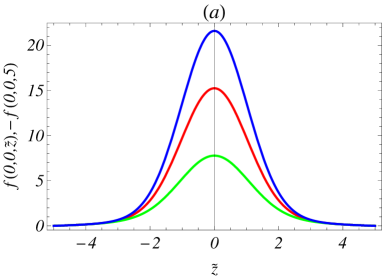
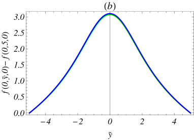
Figure 1: Behavior of $f(\tilde{x},\tilde{y},\tilde{z})$ in Eq. (53) ) for a cylindrical bunch ($\eta=1$): (a) along the $\tilde{z}$ axis and (b) along the $\tilde{y}$ axis . Blue: $\alpha=10^{-9}$, Red: $\alpha=5.7\times 10^{-7}$, Green: $\alpha=10^{-3}$.

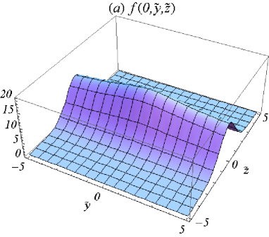
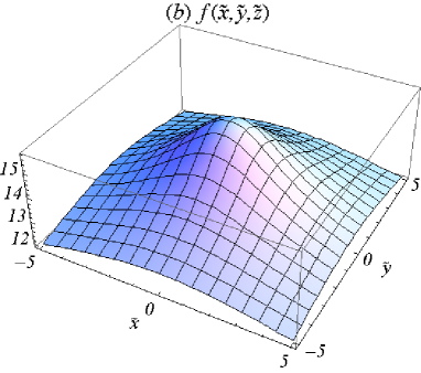
Figure 2: Behavior of $f(\tilde{x},\tilde{y},\tilde{z})$ in Eq. (53) for a cylindrical bunch over (a) the $\tilde{x}=0$ plane and (b) the $\tilde{z}=0$ plane . Here $\eta=1$ and $\alpha=5.7\times 10^{-7}$ as in Eq.  (58).

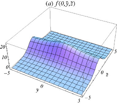
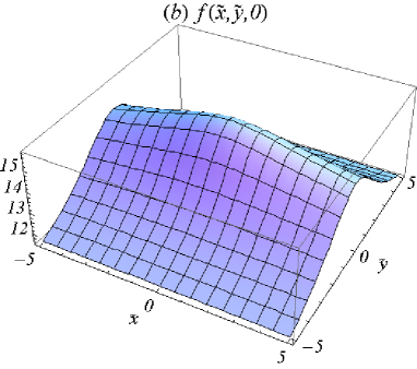
Figure 3: Behavior of $f(\tilde{x},\tilde{y},\tilde{z})$ in Eq. (53) for a flat bunch over (a) the $\tilde{x}=0$ plane and (b) the $\tilde{z}=0$ plane. Here $\eta=0.02$ and $\alpha=1.7\times 10^{-6}$ as in Eq.  (59).

To quantitatively compare the slice potential energy spread with the usual slice kinetic energy spread, and in particular, to compute the slice spread of the total energy, here we use the following parameters for the bunch lcls ; heater

$$\mathcal{E}_{0}=135~{}\mbox{MeV},\sigma_{z}=750\,\mu\mbox{m},\gamma_{0}\epsilon_{x}=\gamma_{0}\epsilon_{y}=1\,\mu\mbox{m}.$$ (57)

with two examples of beta functions at the entrance of a bending system: (i) cylindrical bunch with $\beta_{x}=\beta_{y}=6\,\mbox{m}$ and (ii) flat bunch with $\beta_{x}=0.36\,\mbox{m},\beta_{y}=18\,\mbox{m}$. The potential energy spread for the central slice of the bunch can then be estimated using the rigid-bunch formula Eq. (52) with the following parameters corresponding to the above two cases:

$$\mbox{case i}:\hskip 14.45377pt\eta=1,\hskip 14.45377pt\alpha=5.7\times 10^{-7},$$ (58)

$$\mbox{case ii}:\hskip 14.45377pt\eta=0.02,\hskip 14.45377pt\alpha=1.7\times 10^{-6}.$$ (59)

We will further choose $I_{p}=120$ A and thus $\mathcal{E}_{0}=3.6$ keV, and examine situations when the slice kinetic energy spread takes the typical value $\sigma_{\mathcal{E}_{k}}=3\,\mbox{keV}$ fel08 and a much smaller value $\sigma_{\mathcal{E}_{k}}$= 1 keV (note that for typical LCLS operation the bunch charge is 250 pC, corresponding to $I_{p}=40$ A with $\sigma_{z}=750\,\mu$m).

The calculation of the spread of $\mathcal{E}_{\phi}$ requires the knowledge of the probability distribution of particles over $\mathcal{E}_{\phi}$, i.e., $P_{\mathcal{E}_{\phi}}(\mathcal{E}_{\phi})$. Consider $z=0$ slice of the cylindrical bunch, with the transverse probability distribution

$$P(x,y)dxdy=\frac{1}{2\pi\sigma_{x}\sigma_{y}}\exp\left(-\frac{x^{2}}{2\sigma_{x}^{2}}-\frac{y^{2}}{2\sigma_{y}^{2}}\right)\,dxdy=\frac{1}{2\pi\sigma_{r}^{2}}\exp\left(-\frac{r^{2}}{2\sigma_{r}^{2}}\right)rdrd\phi.$$ (60)

For $w=\tilde{r}^{2}$, the probability for particles to lie between $w$ and $w+dw$ is

$$P_{w}(w)=\frac{1}{2}e^{-w/2},\hskip 14.45377pt\mbox{with}\hskip 14.45377pt\int_{0}^{\infty}P_{w}(w)dw=1.$$ (61)

Then with the one to one correspondence between $w$ and $\mathcal{E}_{\phi}$ following Eq. (88)

$$\mathcal{E}_{\phi}(r,0)=\mathcal{E}_{\phi 0}\,U(w),$$ (62)

with $U$ being the normalized potential energy

$$U(w)=\frac{\mathcal{E}_{\phi}}{\mathcal{E}_{\phi 0}}=\int_{0}^{\infty}\frac{d\tau}{(1+\tau)\sqrt{1+\alpha\tau}}\exp\left(-\frac{w}{2(1+\tau)}\right),\vspace{0.15in}$$ (63)

one gets the probability for the value of potential energy of a particle to reside between $\mathcal{E}_{\phi}$ and $\mathcal{E}_{\phi}+d\mathcal{E}_{\phi}$

$$P_{\mathcal{E}_{\phi}}(\mathcal{E}_{\phi})\,d\mathcal{E}_{\phi}=P_{U}(U)dU=P_{w}(w)dw$$ (64)

or

$$P_{U}(w)\equiv P_{\mathcal{E}_{\phi}}(\mathcal{E}_{\phi})\mathcal{E}_{\phi 0}=\frac{P_{w}(w)}{|dU(w)/dw|}.$$ (65)

We now look at the probability distribution of potential energy of particles for a cylindrical Gaussian bunch. With $\eta=1$ and $\alpha=5.7\times 10^{-7}$ as in Eq. (58), we plot $U(w)$ and $P_{U}(w)$ in Fig. 4, which shows that $U$ reaches its maximum value $U_{m}=U(0)=15.8$ at $w=0$. The semi-analytical results of $P_{U}$ on $U$ is shown as the solid brown curve in Fig. 5, as obtained from the parametric dependence of $(U(w),P_{U}(w))$ on $w$. The domain of the function $P_{U}(U)$ is $(0,U_{m})$. In our study the function $P_{U}(U)$ is obtained by interpolating an array $(U(w_{i}),P_{U}(w_{i}))$, with $w_{i}$ an equally spaced array in range $[0,\,25]$ corresponding to $\tilde{r}$ in the range $[0,5]$. Numerically it can be verified that $P_{U}(U)$ thus obtained satisfies

$$\int_{0}^{U_{m}}P_{U}(U)dU=1.$$ (66)

Knowing the probability distribution $P_{U}(U)$, one can further find the average and rms width of the particle distribution over $U$:

$$\langle U\rangle=\int_{0}^{U_{m}}P_{U}(U)UdU,\hskip 14.45377pt\mbox{and}\hskip 14.45377pt\sigma_{U}=\sqrt{\langle(\Delta U)^{2}\rangle},$$ (67)

for

$$\langle(\Delta U)^{2}\rangle=\int_{0}^{U_{m}}P_{U}(U)(U-\langle U\rangle)^{2}dU.$$ (68)

Here $\langle U\rangle=15.0$, and $\sigma_{U}$= 0.51. Note that the above results have weak dependence on $\alpha$ since $U(w)$ is insensitive to $\alpha$ as indicated by Fig. 1(b).

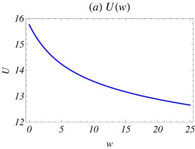
Figure 4: Behavior of $U(w)$ in Eq. (63) and $P_{U}(w)$ in Eq. (65) for a cylindrical bunch ($\eta=1$, $\alpha=5.7\times 10^{-7}$): (a) $U$ vs. $w$ and (b) $P_{U}$ vs. $w$.

Finally, we calculate the spread of the total slice energy spread for the $z=0$ slice because the observed dynamical effect on a bunch moving through a bending system is always related to the distribution of the initial total energy offset of the particles. The total energy offset from the design energy $\mathcal{E}_{0}$ for a particle is

$$\Delta\mathcal{E}=\Delta\mathcal{E}_{k}+\mathcal{E}_{\phi}\hskip 14.45377pt\mbox{for}\hskip 14.45377pt\Delta\mathcal{E}_{k}=\mathcal{E}_{k}-\mathcal{E}_{0},$$ (69)

with $\mathcal{E}_{\phi}=\mathcal{E}_{\phi 0}\,U$, and $\mathcal{E}_{k}$ being the initial kinetic energy. Assuming the probability of the kinetic energy distribution is Gaussian

$$P_{\mathcal{E}_{k}}(\Delta\mathcal{E}_{k})=\frac{1}{\sqrt{2\pi}\sigma_{\mathcal{E}_{k}}}\exp\left(-\frac{(\Delta\mathcal{E}_{k})^{2}}{2(\sigma_{\mathcal{E}_{k}})^{2}}\right),$$ (70)

then the probability of particle distribution $P_{\mathcal{E}}(\Delta\mathcal{E})$ over $\Delta\mathcal{E}$ is related to $P_{\mathcal{E}k}(\Delta\mathcal{E}_{k})$ and $P_{U}(U)$ by rdm

$$P_{\mathcal{E}}(\Delta\mathcal{E}) = \int_{0}^{\mathcal{E}_{\phi m}}P_{\mathcal{E}_{k}}(\Delta\mathcal{E}-\mathcal{E}_{\phi})P_{\mathcal{E}_{\phi}}(\mathcal{E}_{\phi})\,d\mathcal{E}_{\phi}$$ (71)

$$= \int_{0}^{U_{m}}P_{\mathcal{E}_{k}}(\Delta\mathcal{E}-\mathcal{E}_{\phi 0}U)P_{U}(U)\,dU.$$

The average $\langle\mathcal{E}\rangle$ and root mean square (rms) $\sigma_{\mathcal{E}}$ of $P_{\mathcal{E}}(\Delta\mathcal{E})$ distribution can be further calculated. An estimation of $\sigma_{\mathcal{E}}$ is given by

$$\bar{\sigma}_{\mathcal{E}}\simeq\sqrt{(\sigma_{\mathcal{E}_{k}})^{2}+(\mathcal{E}_{\phi 0}\,\sigma_{U})^{2}}.$$ (72)

This relation shows that the rms of the joint energy can be appreciably larger than that of the kinetic slice energy spread when

$$\xi\equiv\frac{\mathcal{E}_{\phi 0}\,\sigma_{U}}{\sigma_{\mathcal{E}_{k}}}\geq 1,$$ (73)

which often implies high peak current $I_{p}$ and small kinetic energy spread $\sigma_{\mathcal{E}_{k}}$.

For the parameters in Eq. (58), the probability distribution of the joint energy offset $P_{\mathcal{E}}(\Delta\mathcal{E})$ can be obtained from Eq. (71) by applying $P_{\mathcal{E}_{k}}(\Delta\mathcal{E}_{k})$ in Eq. (70) and the semi-analytical result of $P_{U}(U)$. The final results are shown in Fig. 6 for two cases, $\sigma_{\mathcal{E}_{k}}=3$  keV for Fig. 6(a) when $\xi=0.6$, and $\sigma_{\mathcal{E}_{k}}=1$  keV for Fig. 6(b) when $\xi=1.8$ . As expected the latter case demonstrates clear effect of slice potential energy spread on the widening of the slice total energy spread. Here the solid green lines are the Gaussian probability distribution for the slice kinetic energy offset $\Delta\mathcal{E}_{k}$ as given by Eq. (70), the solid brown lines are the semi-analytical results of probability distribution for the joint energy offset as given by Eq. (71), and the solid black lines are the Gaussian distribution using the estimated rms in Eq. (72). As an example, for $\sigma_{\mathcal{E}_{k}}=1$  keV in Fig. 6(b), we find the rms of $P_{\mathcal{E}}(\Delta\mathcal{E})$ is $\sigma_{\mathcal{E}}=2.09$ keV, which agrees with the approximation by Eq. (72) (for $\mathcal{E}_{\phi 0}=3.6$  keV and $\langle U\rangle=0.51$). The asymmetric feature of $P_{\mathcal{E}}(\Delta\mathcal{E})$, as apparently shown by the solid brown lines in Fig. 6(b), can be explained by the asymmetric feature of $P_{U}(U)$ about $\langle U\rangle$ in Fig.  5, as the result of the fact that particles are more likely to populate at smaller values of $r$ where $U$ takes larger value ($U$ is always positive).

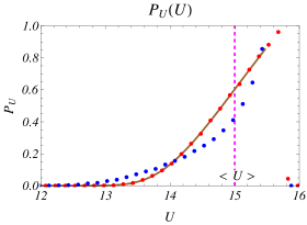
Figure 5: $P_{U}(U)$ for the central slice of a Gaussian bunch. For the cylindrical bunch with $\eta=1$ and $\alpha=5.7\times 10^{-7}$, results are shown by the solid brown line (semi-analytical method) and the red dots (Monte Carlo method). For the flat bunch with $\eta=0.02$ and $\alpha=1.7\times 10^{-6}$, results are shown by the blue dots (Monte Carlo method).

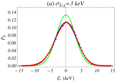
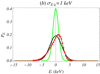
Figure 6: $P_{\mathcal{E}}(\Delta\mathcal{E})$ for the central slice of a cylindrical Gaussian bunch with $\mathcal{E}_{\phi 0}=3.6$  keV, $\eta=1$, $\alpha=5.7\times 10^{-7}$ for (a) $\sigma_{\mathcal{E}}=3$  keV and (b) $\sigma_{\mathcal{E}}=1$  keV. Green line: Gaussian distribution for $\Delta\mathcal{E}_{k}$; Brown line: semi-analytical results of probability distribution for $\Delta\mathcal{E}$; Black line: Gaussian distribution for $\Delta\mathcal{E}$ with estimated rms in Eq. (72); Red dots: Monte Carlo results of probability distribution for $\Delta\mathcal{E}$.

For a cylindrical Gaussian bunch, the semi-analytical results for the probability distributions of the potential and total energy of the particles, shown in Fig. 5 and Fig. 6 respectively, can be verified by the Monte Carlo approach. In this approach we populate $N$ particles in the 2D configuration space $(\tilde{x},\tilde{y})$ for the $z=0$ slice and in the kinetic energy offset $\Delta\mathcal{E}_{k}$ with random Gaussian distribution. The potential energy of each particle can be evaluated from Eq. (52) by $\mathcal{E}_{\phi}^{i}=\mathcal{E}_{\phi}(x^{i},y^{i},z^{i}=0)$, and subsequently the total energy offset of the particle is $\Delta\mathcal{E}^{i}=\Delta\mathcal{E}_{k}^{i}+\mathcal{E}_{\phi}^{i}$, with superscript $i$ denoting the $i$-th particle. One then finds $P_{U}(U)$ and $P_{\mathcal{E}}(\Delta\mathcal{E})$ from the histogram of $\mathcal{E}_{\phi}^{i}$ and $\Delta\mathcal{E}^{i}$ for all particles. Same approach can also be applied to flat bunch case in Eq. (59). Here we set $N=100000$. For cylindrical bunch as in Eq. (58), the Monte Carlo results are shown by the red dots in Fig. 5 for $P_{U}(U)$ and in Fig. 6 for $P_{\mathcal{E}}(\Delta\mathcal{E})$, which are all in good agreement with the semi-analytical results depicted by the solid brown curves in Figs.  5 and 6. For a flat bunch with $\eta=0.02$, the Monte Carlo results are shown as the blue dots in Fig. 5 and Fig. 7. Here part of Fig. 6(b) is replotted in Fig. 7 for $\eta=1$ and compared with the results for $\eta=0.02$. This comparison shows that the probability distribution for total energy of particles is more asymmetric for a flat bunch than that for a cylindrical bunch when Eq. (73) is satisfied.

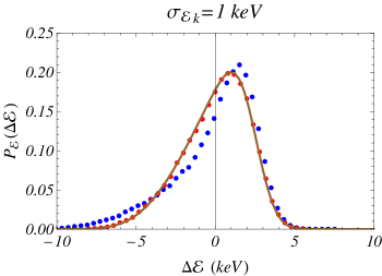
Figure 7: $P_{\mathcal{E}}(\Delta\mathcal{E})$ for the central slice of a Gaussian bunch with $\sigma_{\mathcal{E}}=1$  keV and $\mathcal{E}_{\phi 0}=3.6$  keV. The solid brown line is for semi-analytical result and the red dots are for the Monte Carlo result ($\eta=1,\alpha=5.7\times 10^{-7}$). The blue dots are for the Monte Carlo result of the flat bunch case ($\eta=0.02,\alpha=1.7\times 10^{-6})$.

IV Discussions

For an electron bunch being transported through a magnetic bending system, we have shown in Sec. II that the energy spread of the bunch observed in dispersive regions and the bunch length determined by momentum compaction of the bending system are actually related to the spread of the total (or canonical) energy $\mathcal{E}=\mathcal{E}_{k}+\mathcal{E}_{\phi}$ of the particles in the bunch instead of the spread of the kinetic energy $\mathcal{E}_{k}$ of the particles alone as previously assumed. The spread of $\mathcal{E}_{\phi}$ is called pseudo energy spread since the measurements may give the appearance of a larger kinetic energy spread as a result of the pseudo energy spread. In Sec. III, by analyzing the probability distribution $P_{\mathcal{E}}(\Delta\mathcal{E})$ of the total energy offset from design energy for the central ($z=0$) slice of a rigid cylindrical Gaussian bunch moving relativistically on a straight path, we find that the contribution of ${\mathcal{E}_{\phi}}$ to the total energy spread can be appreciable when Eq. (73) is satisfied, i.e., when a bunch has high peak current and low slice kinetic energy spread. In this section, the implication of pseudo slice energy spread for bunch dynamics in bends, including microbunching instability, will be discussed. Other effects not included in this study that requires further consideration will also be highlighted.

IV.1 Effects Not Included in this Study

First, the present study assumes free-space boundary condition. The existence of wave-guide boundary will alter the functional form of $\mathcal{E}_{\phi}(x,y,z)$ by adding a solution of homogeneous wave equation to the free-space potential. Despite this modification, the sensitive dependence of $\mathcal{E}_{\phi}$ on $(x,y)$ will preserve since it originates from local interaction.

Second, this study emphasizes on the driving term $G_{\phi 0}$ in Eq. (42), yet the impact of effective CSR forces, which tend to generate correlated (with $z$) phase space distortions in bending systems, are not considered. For 1D steady-state CSR interaction, one has $d\Phi^{\mbox{\scriptsize col}}/dt=0$ and $dA_{r}^{\mbox{\scriptsize col}}/dt=0$, and the behavior of $F_{v}^{\mbox{\scriptsize eff}}$ and $F_{r}^{\mbox{\scriptsize eff}}$ are analyzed derb2 , with the effect of $F_{v}^{\mbox{\scriptsize eff}}$ on transverse dynamics dominant over that of $F_{r}^{\mbox{\scriptsize eff}}$ hbb . A study of the effect of 2D dynamics lir08 on longitudinal effective CSR force $F_{v}^{\mbox{\scriptsize eff}}$ shows that using an actual evolving bunch rather than a rigid line bunch could lead to a delayed response of $F_{v}^{\mbox{\scriptsize eff}}$ to the bunch length variation. In addition, $F_{v}^{\mbox{\scriptsize eff}}$ could be sensitive to the transverse particle coordinates for a short duration around roll-over compression, as a result of sensitivity of longitudinal phase to transverse particle positions when Derbenev criterion derb2 is not satisfied. So the resulting integrated effect of $F_{v}^{\mbox{\scriptsize eff}}$ can have transverse dependence only after role-over compression. The general effect of $F_{r}^{\mbox{\scriptsize eff}}$, including the contribution from $dA_{r}^{\mbox{\scriptsize col}}/dt$ term, requires further investigation. Presently the measured emittance growth in chicanes show good agreement with start-to-end simulations using Elegant bane . This does not contradict with our newly introduced $\mathcal{E}_{\phi}$ term, since just as the initial slice kinetic energy spread, the $\mathcal{E}_{\phi}$ term does not cause emittance growth in an achromatic bending systems.

Third, in general, $P_{\mathcal{E}}(\Delta\mathcal{E})$ depends on the 3D density distribution of the bunch and the history of bunch 3D dynamics. In actual machines the bunch phase space distribution can have complicated structures, as seen in many start-to-end simulations tesla ; ding . Thus detailed studies of the dependence of potential energy on the spatial coordinates are needed for each experimental setting, which may show behavior of the potential energy distribution very different from that for a perfect 3D Gaussian bunch as discussed in this paper. Note that our focus here is on the pseudo slice energy spread for the central slice of the Gaussian bunch, and its dependence on the longitudinal position of the slice is not considered in this paper (it gets smaller for larger $z$ as shown in Figs. 2(a) and 3(a)). Likewise, the maximum value of potential energy $\mathcal{E}_{\phi m}$ for each slice varies with $z$, rendering a curvature of $\mathcal{E}_{\phi m}$ vs. $z$ similar to the effect of RF curvature on beam longitudinal phase space distribution. It remains to be examined whether the curvature of potential energy is always negligible compared to the RF curvature in experiments of interest.

Finally, one should note that in an ideal numerical simulation the cancellation is realized by taking full account of the transverse and longitudinal Lorentz forces, including their local and long range behaviors, and let the dynamics play out with full self-consistency. In this way the interplay of effects from the longitudinal and transverse forces can be faithfully represented, the cancellation can be manifested, and the effect of the pseudo (kinetic) energy term can be revealed. Such interplay may often misrepresented if only partial effects are included.

IV.2 Roles of $\mathcal{E}_{\phi}$ in Experimental Measurement

As we have discussed, the effects of the pseudo slice energy spread are measurable in experiments only for special cases when the bunch peak current is high and the slice kinetic energy spread is low. For a rigid Gaussian bunch the criterion is given by Eq. (73). In most of the existing experiments, the parameters are such that this effect may not be significant. Nonetheless, as the community is pushing for higher peak current and higher brightness of electron beams, this effect may show up in certain future experiment. Here we make some general comments of its possible impact on bunch dynamics in bending systems.

A common scheme for measuring the slice energy spread is to use the transverse deflecting RF structure (TDS) together with a spectrometer tds . According to the Panofsky-Wenzel theorem, TDS can introduce additional local energy spread to the beam. Further evaluations are required to check if the potential energy distribution over the streaked bunch at the entrance of the spectrometer can cause detectable perturbation to the measurement of the slice kinetic energy spread.

Recently measurement of local energy spread was successfully carried out using the coherent harmonic generation (CHG) method chg . In this scheme, an electron bunch is first modulated by $\Delta E=\Delta\gamma\sin z$ with a seeded laser in an undulator, and then is sent through a chicane where energy modulation is converted to density modulation. A second undulator is followed in which microbunched beam generates powerful coherent harmonic radiation, with CHG power $E_{\mbox{\scriptsize CHG}}$ related to the bunching factor $b_{n}$ by $E_{\mbox{\scriptsize CHG}}\propto b_{n}^{2}$. Here the bunching factor at the exit of the chicane is obtained from particle’s coordinates $(x_{0},y_{0},z_{0})$ at the entrance of the chicane via

$$z=z_{0}+R_{56}\left(\frac{\Delta\gamma\sin z}{\gamma}+\frac{\mathcal{E}_{k}}{\gamma mc^{2}}\right).$$ (74)

However, with our present results of $\mathcal{E}_{\phi}$ effect on longitudinal optics, we will have

$$z=z_{0}+R_{56}\left(\frac{\Delta\gamma\sin z}{\gamma}+\frac{\Delta\mathcal{E}_{k}+\mathcal{E}_{\phi}(x_{0},y_{0},z_{0})}{\gamma mc^{2}}\right),$$ (75)

and the bunching factor can be obtained by including additional integration over transverse density distribution. For the recent measurement chg , with bunch charge 100 pC and (FWHM) pulse length 8 ps, we have $\mathcal{E}_{\phi 0}=0.35$  keV or $\xi\sim 0.18$ . Therefore perturbation on the kinetic energy spread ($\sigma_{k}\sim 1$ keV) from $\mathcal{E}_{\phi}$ is negligible if a rigid cylindrical Gaussian bunch is used for a rough estimation. In general, magnetic chicanes are commonly used in the CHG experiments as well as the HGHG and EEHG eehg experiments, in which slice energy spread is a crucial parameter. In case the bunch peak current is pushed to the point when Eq. (73) is satisfied, special care is required to evaluate the effects of $\mathcal{E}_{\phi}$ on the final bunching factor and efficiency of these schemes for high harmonic numbers.

At high peak current, the pseudo slice energy spread $\mathcal{E}_{\phi}$ can also have impact on the longitudinal space charge induced microbunching instability, developed on a beamline consisting of a straight section followed by a chicane. Note that even for cases with the kinetic energy spread comparable with the potential energy spread, the contributions of $\mathcal{E}_{k}$ and $\mathcal{E}_{\phi}$ to the final bunching factor can be quite different, because $\exp(ikR_{56}\mathcal{E}_{\phi}(x_{0},y_{0},z_{0})/\mathcal{E}_{0})$ in Eq. (75) will be averaged over transverse spatial distribution, yet $\mathcal{E}_{k}$ is averaged over the energy distribution.

The emphasis of this paper is that the pseudo slice energy spread plays an equal role with the kinetic energy spread in their contribution to the measured values of the energy spread in dispersive regions and to the minimum bunch length at full compression when the bunch is transported through a magnetic bending system. It would be interesting to demonstrate this effect of pseudo slice energy spread with clarity by creating an experimental condition of high peak bunch current and low slice kinetic energy spread. Such condition may require an emittance exchange from the longitudinal phase space to the transverse phase space, which is a process reversed from the usual practice, namely, converting the transverse phase space emittance to the longitudinal one eex . It is expected that transporting such a beam with low longitudinal phase space emittance through a bending system will allow the pseudo slice energy spread to have pronounced effects in measurements.

It should be noted that many discussions in this paper assume a random Gaussian distribution for the kinetic energy of the particles, while the potential energy of the particles varies depending on the particle coordinates inside the bunch. However, in actual bunch dynamics, the kinetic and potential energies are closely correlated because their sum—the canonical energy—is changed by the effective longitudinal force which in most cases roll only depends on $z$ at ultrarelativistic limit. The correlation between the kinetic and potential energy of particles can be found by a self-consistent start-to-end simulation with all space charge and CSR forces included.

In past years there have been puzzles that sometimes the measured slice energy spread is bigger than the expected value obtained from numerical modeling of beam generation from the gun and beam transport in the injector uBI . There could be various reasons causing this puzzle. Depending on the actual parameters of an experiment, the possible contribution of pseudo slice energy spread to the measured value of slice kinetic energy spread needs to be carefully evaluated and sorted out.

V Conclusion

In this study, for an ultrarelativistic electron bunch being transported through a magnetic bending system, we consider a remnant driving term of particle transverse dynamics after the cancellation between the Talman’s force and the non-inertial space charge force in particle transverse dynamics is taken into account. This driving term is related to the initial potential energy of the particles at the entrance of the bending system, which has sensitive dependence on the transverse coordinates of particles in the bunch, and it does not cause emittance growth for an achromatic bending system. Without careful analysis of the detailed interplay of the longitudinal and transverse CSR forces in particle transverse dynamics, the effect of this term may appear experimentally in disguise as a part of the kinetic energy spread. Our estimation for a cylindrical Gaussian bunch shows that the slice potential energy spread, or pseudo energy spread, can be comparable in magnitude with the slice kinetic energy spread when the bunch peak current is high and the slice kinetic energy spread is small. This result renders the importance in sorting out the possible contribution of $\mathcal{E}_{\phi}$ term from the measured results of slice energy spread. The possible role of $\mathcal{E}_{\phi}$ in various experimental designs involving chicanes are discussed. Finally, we note that the effect of pseudo slice energy spread is not included in the common 1D CSR simulation, and it can only be revealed by an accurate, complete and fully self-consistent CSR interaction model. Further numerical and experimental studies are needed for reaching a more complete and thorough understanding of the effect of pseudo slice energy spread.

Appendix A Retarded Potential

We now analyze the retarded scalar potential on particles for a rigid 3D Gaussian bunch moving on a straight path, and show that the analytical expression of the retarded potential is identical to the scalar potential as obtained by applying Lorentz transformation to the 4-vector potentials from the bunch comoving frame to the lab frame.

Consider an ideal case when a Gaussian bunch moves on a straight path, with all particles moving only longitudinally and at constant velocity $v=\beta c$. The motion of the bunch center is described by $s=\beta ct$. The retarded potential on a test particle at $({\bf x},t)$ is

$$\Phi^{\mbox{\scriptsize col}}({\bf x},t)=\int\frac{\rho({\bf x}_{r},t_{r})}{|{\bf x}-{\bf x}_{r}|}d^{3}{\bf x}_{r},$$ (76)

where $t_{r}=t-|{\bf x}-{\bf x}_{r}|/c$ is the retarded time, and

$$\rho({\bf x}_{r},t_{r})=\frac{Ne}{(2\pi)^{3/2}\sigma_{x}\sigma_{y}\sigma_{z}}\exp\left(-\frac{x_{r}^{2}}{2\sigma_{x}^{2}}-\frac{y_{r}^{2}}{2\sigma_{y}^{2}}-\frac{(s_{r}-\beta ct_{r})^{2}}{2\sigma_{z}^{2}}\right).$$ (77)

Here $(x_{r},y_{r},s_{r})$ are the Cartesian coordinates of a source particle in the lab frame, and $N$ is the number of electrons in the bunch.

Let $z=s-\beta ct$ be the longitudinal position of the test particle relative to the bunch center. For $\Delta s=s-s_{r}$, we have for the source particle

$$z_{r}=s_{r}-\beta ct_{r}=z-\Delta s+\beta|{\bf x}-{\bf x}_{r}|.\vspace{-0.1in}$$ (78)

With the identities math

$$\frac{1}{\sqrt{2\pi}\sigma_{z}}\exp\left(-\frac{(s_{r}-\beta ct_{r})^{2}}{2\sigma_{z}^{2}}\right)=\frac{1}{\pi}\mbox{Re}\int_{0}^{\infty}\exp\left[-\frac{k^{2}\sigma_{z}^{2}}{2}+i[k(z-\Delta s)+k\beta|{\bf x}-{\bf x}_{r}|]\right]\,dk\vspace{0.1in}$$ (79)

and

$$\frac{\exp(ik\beta|{\bf x}-{\bf x}_{r}|)}{|{\bf x}-{\bf x}_{r}|}=\frac{1}{\pi}\int_{0}^{\infty}\exp\left[i\left((k\beta u)^{2}+\frac{|{\bf x}-{\bf x}_{r}|^{2}}{4u^{2}}-\frac{\pi}{4}\right)\right]\frac{du}{u^{2}},\vspace{0.1in}$$ (80)

and with the new variable $w=u^{2}$, $\Phi^{\mbox{\scriptsize col}}({\bf x},t)$ in Eq. (76) becomes ${\it\Phi}(x,y,z)$ in terms of particle coordinates internal to the bunch

$${\it\Phi}(x,y,z) = \mbox{ Re}\left\{\frac{i}{\sqrt{2\pi}}\int_{0}^{\infty}\frac{dw}{\sqrt{(\sigma_{x}^{2}+iw)(\sigma_{y}^{2}+iw)(\sigma_{z}^{2}+iw/\gamma^{2})}}\right.$$ (81)

$$\left.\times\exp\left[-\frac{x^{2}}{2(\sigma_{x}^{2}+iw)}-\frac{y^{2}}{2(\sigma_{y}^{2}+iw)}-\frac{z^{2}}{2(\sigma_{z}^{2}+iw/\gamma^{2})}\right]\right\}.$$

Here the path of integration for $iw$ is $C_{1}$ in Fig. 8. For the above integrand, we have in Fig. 8 $\int_{C_{1}}+\int_{C_{R}}+\int_{C_{2}}=0$, as well as $\int_{C_{R}}=0$ for $R\rightarrow\infty$. This allows us to replace $\int_{C_{1}}$ by $-\int_{C_{2}}$, or

$${\it\Phi}(x,y,z) = \frac{Ne}{\sqrt{2\pi}\sigma_{z}}\int_{0}^{\infty}\frac{d\tau}{\sqrt{(\tau+\eta)(\tau+1)(1+\alpha\tau)}}$$ (82)

$$\times\exp\left(-\frac{\tilde{x}^{2}}{2(1+\tau/\eta)}-\frac{\tilde{y}^{2}}{2(1+\tau)}-\frac{\tilde{z}^{2}}{2(1+\alpha\tau)}\right)$$

for $(\tilde{x},\tilde{y},\tilde{z})=(x/\sigma_{x},y/\sigma_{y},z/\sigma_{z})$, along with $\eta=(\sigma_{x}/\sigma_{y})^{2}$ and $\alpha=(\sigma_{y}/\gamma\sigma_{z})^{2}$.

Next we show that Eq. (82) can be obtained by applying Lorentz transformation on the scalar potential from the bunch comoving frame to the lab frame. In the comoving frame, let $(x^{\prime},y^{\prime},s^{\prime})$ be the particle coordinates, $\Phi^{\prime}$ be the scalar potential, and let the rms bunch length be $\sigma^{\prime}_{x},\sigma^{\prime}_{y}$ and $\sigma^{\prime}_{z}$. One has kheifets

$$\Phi^{\prime}({\bf x^{\prime}})=\int d{\bf y^{\prime}}\frac{\rho({\bf y^{\prime}})}{|{\bf x^{\prime}}-{\bf y^{\prime}}|}=\frac{Ne}{\sqrt{\pi}}\int_{0}^{\infty}\frac{du}{\sqrt{(u+2\sigma_{x}^{2})(u+2\sigma_{y}^{2})(u+2\sigma_{z}^{2})}}\\ \times\exp\left(-\frac{x^{\prime 2}}{u+2\sigma_{x}^{{}^{\prime}2}}-\frac{y^{\prime 2}}{u+2\sigma_{y}^{{}^{\prime}2}}-\frac{s^{\prime 2}}{u+2\sigma_{z}^{{}^{\prime}2}}\right).$$ (83)

Combining $\Phi^{\prime}({\bf x^{\prime}})$ in Eq. (83) with the Lorentz transformation, i.e., $\Phi^{\prime}=\gamma\Phi$, $s^{\prime}=\gamma(s-\beta ct)\equiv\gamma z,x^{\prime}=x,y^{\prime}=y$, together with $\sigma^{\prime}_{z}=\gamma\sigma_{z},\sigma^{\prime}_{x}=\sigma_{x},\sigma^{\prime}_{y}=\sigma_{y}$ and $u=2\sigma_{y}^{2}\tau$, one gets the scalar potential in the lab frame

$$\Phi(x,y,s,t)={\it\Phi}(x,y,z)=\int d{\bf x}_{1}\frac{\rho({\bf x}_{1})}{|{\bf x}-{\bf x}_{1}|}=\frac{Ne}{\sqrt{2\pi}\sigma_{z}}\int_{0}^{\infty}\frac{d\tau}{\sqrt{(\tau+\eta)(\tau+1)(\alpha\tau+1)}}\\ \times\exp\left(-\frac{\tilde{x}^{2}}{2(\tau/\eta+1)}-\frac{\tilde{y}^{2}}{2(\tau+1)}-\frac{\tilde{z}^{2}}{2(\alpha\tau+1)}\right)$$ (84)

which is identical to the retarded potential in Eq. (82) as expected.

The potential energy of an electron at coordinate $(x,y,z)$ within the bunch is

$$\mathcal{E}_{\phi}(x,y,z)\equiv e{\it\Phi}(x,y,z)=\mathcal{E}_{\phi 0}f(\tilde{x},\tilde{y},\tilde{z})\hskip 14.45377pt\mbox{with}\hskip 14.45377pt\mathcal{E}_{\phi 0}=mc^{2}\frac{I_{p}}{I_{A}},$$ (85)

for $I_{p}=Nec/(\sqrt{2\pi}\sigma_{z})$ being the peak current and $I_{A}=e/(r_{e}c)$=17 kA the Alfven current, and

$$f(\tilde{x},\tilde{y},\tilde{z})=\int_{0}^{\infty}\frac{d\tau}{\sqrt{(\tau+\eta)(\tau+1)(\alpha\tau+1)}}\exp\left[-\frac{\tilde{x}^{2}}{2(\tau/\eta+1)}-\frac{\tilde{y}^{2}}{2(\tau+1)}-\frac{\tilde{z}^{2}}{2(\alpha\tau+1)}\right].$$ (86)

For a cylindrical beam, $\sigma_{x}=\sigma_{y}=\sigma_{r}$, and $\tilde{r}^{2}=\tilde{x}^{2}+\tilde{y}^{2}$. Then $\mathcal{E}_{\phi}(x,y,z)$ becomes $\mathcal{E}_{\phi c}(r,z)$

$$\mathcal{E}_{\phi c}(r,z)=\mathcal{E}_{\phi 0}f_{c}(\tilde{r},\tilde{z})\vspace{-0.05in}$$ (87)

for

$$f_{c}(r,z)=\int_{0}^{\infty}\frac{d\tau}{(1+\tau)\sqrt{1+\alpha\tau}}\exp\left(-\frac{\tilde{r}^{2}}{2(1+\tau)}-\frac{\tilde{z}^{2}}{2(1+\alpha\tau)}\right).\vspace{0.1in}$$ (88)

This expression is identical to Eq. (2) of Ref. accl with $\tau^{-1}=\lambda^{2}\sigma_{\perp}^{2}$.

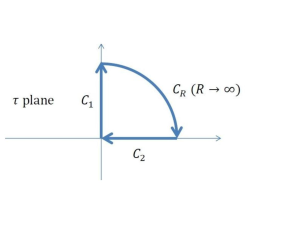
Figure 8: contour

For an infinitely long bunch, $\alpha=0$ and thus the integral in Eq. (88) diverges. Even though this integral converges for a realistic beam of finite $\alpha$, the numerical integration converges very slowly as the upper limit approaches infinity. To increase the convergence rate for numerical computation, we change the variable from $\tau$ to $\kappa$ by $\kappa=\sinh^{-1}(\alpha\tau)$. Eq. (86) becomes

$$f(\tilde{x},\tilde{y},\tilde{z}) = \int_{0}^{\infty}\frac{\cosh\kappa\,d\kappa}{\sqrt{(\alpha\eta+\sinh\kappa)(\alpha+\sinh\kappa)(1+\sinh\kappa)}}$$ (89)

$$\times\exp\left(-\frac{\alpha\,\tilde{x}^{2}}{2(\alpha+\sinh\kappa/\eta)}-\frac{\alpha\,\tilde{y}^{2}}{2(\alpha+\sinh\kappa)}-\frac{\tilde{z}^{2}}{2(1+\sinh\kappa)}\right),$$

where $f(\tilde{x},\tilde{y},\tilde{z})$ reaches its convergent result when the upper limit of integral $\kappa_{\mbox{\scriptsize max}}\sim 30$. For the potential energy of particles in the central slice of a cylindrical bunch, we set $\eta=1$ and $\tilde{z}=0$ in Eq. (89). Using $U(\omega)$ to represent the dependence of $f_{c}(r,0)$ in Eq. (88) on $\omega=\tilde{r}^{2}$, we get

$$U(\omega)=\int_{0}^{\infty}\frac{\cosh\kappa d\kappa}{(\alpha+\sinh\kappa)\sqrt{1+\sinh\kappa}}\exp\left(-\frac{\alpha\,\omega}{2(\alpha+\sinh\kappa)}\right).$$ (90)

The behavior of $U(\omega)$ is shown in Fig. 63. The form function for the probability of $\mathcal{E}_{\phi}$ over $\omega$ is given by Eq. (65), where $dU/dw$ can be deduced from Eq. (90).

References

- (1) E. L. Saldin, E. A. Schneidmiller and M. V. Yurkov, TESLA-FEL-2003-02, 2003.
- (2) S. Heifets, G. Stupakov, and S. Krinsky, Phys. Rev. ST Accel. Beams 5, 064401 (2002);
- (3) Z. Huang and K. Kim, Phys. Rev. ST Accel. Beams 5, 074401 (2002).
- (4) M. Hüning and H. Schlarb, in Proceedings of PAC 2003, Portland (2003).
- (5) D. Ratner, A. Chao, and Z. Huang, Proceedings of FEL08, Gyeongju, Korea, (2008).
- (6) C. Feng et al., Phys. Rev. ST Accel. Beams 14, 090701 (2011) .
- (7) R. Li, Proceedings of the 2nd ICFA Advanced Accelerator Workshop, p.369 (1999).
- (8) R. Li, Proceedings of 2002 EPAC, p. 1365, Paris (2002).
- (9) R. Li and Ya. Derbenev, JLAB-TN-02-054 (2002).
- (10) R. Li, Proceedings of the 2003 Particle Accelerator Conference, p. 208, Portland (2003).
- (11) R. Li and Ya. Derbenev, Proceedings of 2005 Particle Accelerator Conference, p. 1631, Knoxville (2005).
- (12) R. Li, Phys. Rev. ST Accel. Beams 11, 024401 (2008).
- (13) G. Stupakov, SLAC-PUB-8683, (2000).
- (14) Ya. S. Derbenev and V. D. Shiltsev, SLAC-Pub-7181 (1996).
- (15) Exception is found for the short duration of beam transport around roll-over compression lir08 .
- (16) G. Bassi, J. Ellison, K. Heinemann, and R.Warnock, Phys. Rev. ST Accel. Beams 13, 104403 (2010).
- (17) R. Talman, Phys. Rev. ST Accel. Beams 7, 100701 (2004).
- (18) R. Talman, Phys. Rev. Lett. 56, 1429 (1986).
- (19) E. Lee, Part. Accel. 25, 241 (1990).
- (20) B. E. Carlsten, PRE, vol.54, p.838 (1996).
- (21) K. L. F. Bane and A. W. Chao, Phys. Rev. ST Accel. Beams 5, 104401, (2002).
- (22) G. Geloni et al., DESY 02-48 and DESY 03-44, (2002).
- (23) M. Borland, Phys. Rev. ST Accel. Beams 4, 070701 (2001).
- (24) G. Stupakov and Z. Huang, SLAC-PUB-12768 (2007).
- (25) R. Akre et al., Phys. Rev. ST Accel. Beams 11, 030703 (2008).
- (26) Z. Huang et al., Phys. Rev. ST Accel. Beams 13, 020703 (2010).
- (27) G. Cooper, C. McGillem, Probabilistic Methods of Signal and System Analysis (1999).
- (28) M. Dohlus, DESY 03-197, arXiv:physics/0312074v1, (2003).
- (29) Y. Ding, PRL 102, 254801 (2009).
- (30) K. L. Bane et. al., Phys. Rev. ST Accel. Beams 12, 030704 (2009).
- (31) D. Xiang and G. Stupakov, PRST-AB, 12, 080701 (2009).
- (32) P. Emma et. al., SLAC-PUB-12038 (2006).
- (33) http://www.umer.umd.edu/events_folder/uBi12/ubi12-Qs/ubi12-Session1/
- (34) S. Kheifets, DESY Report, PETRA-Note 119 (1976).
- (35) I.S. Gradshteyn and I.M. Ryzhik, Table of Integrals, Series, and Products (1979).