Principal trend analysis for time-course data with applications in genomic medicine

Abstract

Time-course high-throughput gene expression data are emerging in genomic and translational medicine. Extracting interesting time-course patterns from a patient cohort can provide biological insights for further clinical research and patient treatment. We propose principal trend analysis (PTA) to extract principal trends of time-course gene expression data from a group of patients, and identify genes that make dominant contributions to the principal trends. Through simulations, we demonstrate the utility of PTA for dimension reduction, time-course signal recovery and feature selection with high-dimensional data. Moreover, PTA derives new insights in real biological and clinical research. We demonstrate the usefulness of PTA by applying it to longitudinal gene expression data of a circadian regulation system and burn patients. These applications show that PTA can extract interesting time-course trends with biological significance, which helps the understanding of biological mechanisms of circadian regulation systems as well as the recovery of burn patients. Overall, the proposed PTA approach will benefit the genomic medicine research. Our method is implemented into an R-package: PTA (Principal Trend Analysis).

T1Supported by P01HG000205 and NIH U54 GM-062119.

and

1 Introduction

High-throughput technologies, such as microarray,LC-MS, next generation sequencing, etc., have been applied widely in current biological and clinical studies. In the past decades, data were usually collected at one time point. Thus, these data have three attributes—feature (gene, protein, etc.), individual (samples, subjects, etc.) and value (gene expression, protein abundance, etc.), which can be represented by matrices with each row indicating feature identity, each column indicating sample identity and each cell recording gene expression or protein abundance. Developing effective ways to analyze such high-throughput genomic and proteomic data is one of the major challenges of bioinformatics and computational biology. In such studies, the number of features $p$ is usually much larger than the number of samples $n$. The lasso method Tibshirani (1996) was introduced and combined with matrix decomposition for computing a rank-$K$ approximation for a matrix; see Zou, Hastie and Tibshirani (2006), Mairal et al. (2010), Witten and Tibshirani (2009), Witten, Tibshirani and Hastie (2009).

The identification of time-course gene/protein expression patterns has attracted increasing attention in biological and clinical research. Time-course genomic and proteomic data have been collected in many clinical and biological studies. It is common for biologists to ask the following question on a set of genes they are interested in: what kinds of dynamic patterns do these genes have? For example, given a group of genes with circadian regulation functions, we want to know their dynamic patterns and their relationships with external light signals. This is important for understanding biological mechanisms in circadian systems, which are critical for maintaining normal living for live organisms. Or in a more unsupervised setting, without preselecting a small set of genes, we want to extract underlying dominant time-course patterns and automatically identify important genes that have contributions on those significant patterns from a genome-wide longitudinal data set. This kind of statistical analysis is especially important for the research of complex diseases, which can provide a systematic view of genomic/proteomic dynamic responses. For example, in a study of host response to burn injuries, clinical investigators monitored a group of burn patients and measured their gene expression over time (www.gluegrant.org). To improve our systematic understanding of the key regulatory elements in the recovery of burn patients, we need to characterize dynamic response in gene expression. To do so, we need a statistical learning approach for high-dimensional longitudinal data to extract underlying time-course patterns and identify important features that contribute to the underlying patterns of interest.

Unlike stationary gene expression data without consideration of time, time-course gene expression data have an additional time attribute. Traditional principal component analysis applied to stationary gene expression data matrix for multiple samples cannot be used directly in this scenario. Thus, dimension reduction methods for time-course data are needed. The method that we propose draws on ideas from the spline-based methods on time-course data analysis [Kimeldorf and Wahba (1970), Wahba (1990)] and principal component analysis for dimension reduction. Our method has the following advantages:

1. Unsupervised approach to automatically discover underlying gene expression time-course patterns.

2. Automatically identifying important genes and classifying them into different groups which contribute to different time-course patterns.

The remainder of this article is organized as follows. Section 2 gives the model and algorithms for principal trend analysis (PTA). Section 3 gives the simulation studies to show the performance of PTA at different scenarios. Section 4 gives an application of PTA on a circadian regulation gene expression data set with a subset of genes as known targets. This data set is from arabidopsis thaliana rosette, which is a widely-used pattern organism. Gene expression was measured six times during 12-h-light/12-h-dark treatments of arabidopsis thaliana rosettes. Section 5 gives an application of PTA on a burn patient gene expression data set without prior information of genes of interest. This study not only shows the usefulness of PTA, but also provide insights for the further research of burn disease. Section 6 discusses the prospective of our methods and future directions.

2 Principal trend analysis

Let $y_{\mathit{npt}}$ denote the gene $p$ expression of subject $n$ at time point $t$, $p\in\{1,\ldots,P\}$, $n\in\{1,\ldots,N\}$, $t\in\{1,\ldots,T\}$. For each gene $p$, $y_{p}$ was centered. We assume all the subjects are from the same population. We want to find the population-level time-course patterns. Thus, we propose a new method called Principal Trend Analysis (PTA) to solve this problem.

We use the following notation. Let $\mathbf{Y}_{n}$ denote a $P\times T$ matrix of observations on subject $n$; $\mathbf{A}$ denote a $P\times K$ matrix of factor scores, $\mathbf{A}=[\mathbf{a}_{1},\ldots,\mathbf{a}_{K}]$, $[\mathbf{A}]_{p,k}=a_{p,k}$; $\bolds{\Theta}$ denote a $K\times(T+2)$ matrix of spline coefficients, $\bolds{\Theta}=[\bolds{\theta}_{1}^{\mathsf{T}},\ldots,\bolds{\theta}_{K}^{\mathsf{T}}]$, $[\bolds{\Theta}]_{k,m}=\theta_{k,m}$; $\mathbf{B}$ denote a $T\times(T+2)$ matrix containing the cubic spline basis, $[\mathbf{B}]_{t,m}=B_{m}(t)$; $\mathbf{S}$ denote a $K\times T$ matrix presenting top $K$ time-course trends across $T$ time points, $[\mathbf{S}]_{k,t}=S_{k}(t)$; and $\mathbf{S}=\bolds{\Theta}\mathbf{B}^{\mathsf{T}}$.

The underlying model is as below:

$$\mathbf{Y}=\left[\matrix{\mathbf{Y}_{1}\cr\mathbf{Y}_{2}\cr\vdots\cr\mathbf{Y}_{N}}\right]=\left[\matrix{\mathbf{A}\bolds{\Theta}\mathbf{B}^{\mathsf{T}}\cr\mathbf{A}\bolds{\Theta}\mathbf{B}^{\mathsf{T}}\cr\vdots\cr\mathbf{A}\bolds{\Theta}\mathbf{B}^{\mathsf{T}}}\right]+\left[\matrix{\mathbf{E}_{1}\cr\mathbf{E}_{2}\cr\vdots\cr\mathbf{E}_{N}}\right].$$ (1)

Let $\hat{\bolds{\Theta}}$ and $\hat{\mathbf{A}}$ denote the parameter estimates of $\bolds{\Theta}$ and $\mathbf{A}$ for model (1). Since both $\bolds{\Theta}$ and $\mathbf{A}$ are unknown, we cannot obtain their least squares solutions simultaneously. Thus, we propose an iterative algorithm to estimate the parameters by solving the following optimization problem:

$$\min_{\mathbf{A},\bolds{\Theta}}L(\mathbf{A},\bolds{\Theta}|\mathbf{Y})\quad\mbox{subject to}$$

(2)

$$\bolds{\Theta}\bolds{\Omega}\bolds{\Theta}^{\mathsf{T}}\leq c_{1},\qquad\|\mathbf{A}\|_{1}\leq c_{2}\quad\mbox{and}\quad\|\mathbf{A}\|_{2}^{2}=1,$$

where $L(\mathbf{A},\bolds{\Theta}|\mathbf{Y})=\sum_{n=1}^{N}\|\mathbf{Y_{n}}-\mathbf{A}\bolds{\Theta}\mathbf{B}^{\mathsf{T}}\|_{F}^{2}$ is a loss function, $\|\cdot\|_{F}$ is the Frobenius norm, $\|\mathbf{A}\|_{1}$ is the nuclear norm of $\mathbf{A}$, $\|\mathbf{A}\|_{2}$ is the euclidean norm of $\mathbf{A}$, $\bolds{\Omega}$ denotes a $(T+2)\times(T+2)$ matrix, and

$$\Omega_{ij}=\int B_{i}^{\prime\prime}(t)B_{j}^{\prime\prime}(t)\,dt.$$

Small values of $c_{1}$ produce smoother curves while larger values produce more wiggly curves. At the one extreme, as $c_{1}\rightarrow 0$, the penalty term dominates, forcing $S_{k}^{\prime\prime}(t)=0$ everywhere, and thus the solution is the least-square line. At the other extreme, as $c_{1}\rightarrow\infty$, the penalty term becomes unimportant and the solution tends to be an interpolating twice-differentiable function.

When $1\leq c_{2}\leq\sqrt{P}$, we obtain sparsity on genes. When $c_{2}>\sqrt{P}$, the Lasso-penalty will be inactive in the condition that $\|\mathbf{A}\|_{2}^{2}\leq 1$.

The optimization problem (2) is not convex due to the $L_{2}$-equality penalty on $\mathbf{A}$. We modify the $L_{2}$-equality penalty in (2) and obtain the following optimization problem:

$$\min_{\mathbf{A},\bolds{\Theta}}L(\mathbf{A},\bolds{\Theta}|\mathbf{Y})\quad\mbox{subject to}$$

$$\bolds{\Theta}\bolds{\Omega}\bolds{\Theta}^{\mathsf{T}}\leq c_{1},\qquad\|\mathbf{A}\|_{1}\leq c_{2}\quad\mbox{and}\quad\|\mathbf{A}\|_{2}^{2}\leq 1.$$

Using Lagrange multipliers, we rewrite the criteria in (2) and (2) as

$$\min_{\mathbf{A},\bolds{\Theta}}L(\mathbf{A},\bolds{\Theta}|\mathbf{Y})+\lambda_{1}\bolds{\Theta}\bolds{\Omega}\bolds{\Theta}^{\mathsf{T}}+\lambda_{2}\|\mathbf{A}\|_{1}+\lambda_{3}\|\mathbf{A}\|_{2}^{2}.$$ (4)

The supplement S1 [Zhang and Davis (2013)] proves that the optimization problem (2) is biconvex, so it can be solved with an iterative algorithm. Moreover, the solution to (2) also satisfies $\|A\|_{2}^{2}=1$, provided that $\lambda_{3}$ is chosen so that (for fixed $\bolds{\Theta}$) the $\mathbf{A}$ that maximizes $\min_{\mathbf{A}}L(\mathbf{A}|\bolds{\Theta},\mathbf{Y})$, subject to $\|\mathbf{A}\|_{1}\leq c_{2}$, has $L_{2}$-norm greater than or equal to 1. This follows from the Karush–Kuhn–Tucker conditions in convex optimization [Boyd and Vandenberghe (2004)]. Thus, for appropriately chosen $\lambda_{3}$, the solutions to (2) solve (2).

If preselected genes are available (e.g., we are interested in one particular pathway or genes with the same biological functions), and the problem is to extract the underlying key time-course trends for these genes, we can remove the lasso penalty in the optimization problem (4), that is, let $\lambda_{2}=0$.

2.1 Algorithm

When $K=1$, we compute the rank-$1$ sparse principal trend (PT) as follows (cf. S2 in the supplementary material [Zhang and Davis (2013)] for the derivation):

1. Initialize $\bolds{\theta}^{(1)}$ and $\mathbf{a}^{(1)}$ with $\|\mathbf{a}\|_{2}=1$.

2. For $i=1,2,\ldots\,$, until convergence:

   1. [(a)]

   2. $\bolds{\theta}^{(i+1)}\leftarrow(N\mathbf{B}^{\mathsf{T}}\mathbf{B}\otimes\mathbf{a}^{(i)\mathsf{T}}\mathbf{a}^{(i)}+\lambda_{1}\bolds{\Omega})^{-1}\mathbf{B}^{\mathsf{T}}(\sum_{n=1}^{N}\mathbf{Y}_{n})\mathbf{a}^{(i)}$.

   3. When $\lambda_{2}=0$,
      $\mathbf{a}^{(i+1)}\leftarrow(\sum_{n=1}^{N}\mathbf{Y}_{n})\mathbf{B}\bolds{\theta}^{(i)}$,
      $\mathbf{a}^{(i+1)}\leftarrow\frac{\mathbf{a}^{(i+1)}}{\|\mathbf{a}^{(i+1)}\|_{2}}$.
      When $\lambda_{2}>0$,
      $\mathbf{a}^{(i+1)}\leftarrow\operatorname{Soft}((\sum_{n=1}^{N}\mathbf{Y}_{n})\mathbf{B}\bolds{\theta}^{(i)},\frac{1}{2}\lambda_{2})$, where $\operatorname{Soft}(\cdot)$ denote the soft thresholding operator; that is, $\operatorname{Soft}(x,c)=\operatorname{sgn}(x)(|x|-c)_{+}$, where $c>0$ is a constant and $x_{+}$ is defined to equal $x$ if $x>0$ and 0 if $x\leq 0$.
      $\mathbf{a}^{(i+1)}\leftarrow\frac{\mathbf{a}^{(i+1)}}{\|\mathbf{a}^{(i+1)}\|_{2}}$.

For multiple component decomposition with $1<K\leq\min\{P,T\}$, we compute the rank-$K$ sparse time-course PT analogously.

For $k\in\{1,\ldots,K\}$, iterate the following procedure:

1. Let $\mathbf{Y}_{n}^{1}\leftarrow\mathbf{Y}_{n}$, for every $n\in\{1,\ldots,N\}$.

2. For $k\in\{1,\ldots,K\}$:

   1. [(a)]

   2. Obtain $\bolds{\theta}_{k}$ and $\mathbf{a}_{k}$ using the single component decomposition algorithm.

   3. $\mathbf{Y}_{n}^{k+1}\leftarrow\mathbf{Y}_{n}^{k}-\mathbf{a}_{k}\bolds{\theta}_{k}\mathbf{B}^{\mathsf{T}}$.

The PTA algorithm is not guaranteed to get the global minimum similar to De Leeuw and Michailidis (1994), but behaves well in practice. We illustrate the effect of parameters by a simple example. We simulate a data set with 9 features, 7 time points and 1 replicate. Values for the first 5 features are drawn from $\sin(2\pi t)+N(0,0.1)$, and those for the remaining 4 features are drawn from $N(0,0.1)$. Raw data is shown in the top-left panel of Figure 1, with each row indicating one feature and each column indicating one time point. The top-right

Figure 1: Effects of tuning parameters for PTA. Top-left panel: raw data, with each row indicating one feature, each column indicating one time point; top-right panel: paths of the coefficient vector $\bolds{\theta}$ according to changes of tuning parameter $\lambda_{1}(\lambda_{1}\in\{0.0001,0.1,1,10\})$ with $\lambda_{2}$ fixed to 2; bottom-left panel: four estimated time-course trends ($\mathbf{S}=\mathbf{B}\bolds{\theta}$, indicated by 1, 2, 3, 4) according to the coefficients and parameters in top-right panel with $\lambda_{1}$ equaling to 0.0001, 0.1, 1 and 10, respectively; bottom-right panel: paths of coefficient vector $a$ according to changes of tuning parameter $c_{2}$ with $\lambda_{1}=1$.

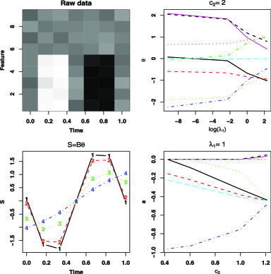
panel of Figure 1 shows how the coefficient vector $\bolds{\theta}$ changes according to tuning parameter $\lambda_{1}(\lambda_{1}\in\{0.0001,0.1,1,10\})$ with $\lambda_{2}$ fixed at 2. The bottom-left panel of Figure 1 shows the estimated time-course trends with $\lambda_{1}$ equal to 0.0001, 0.1, 1 and 10, respectively. One can see that smaller values of $\lambda_{1}$ (larger values of $c_{1}$) produce more wiggly curves, while larger values of $\lambda_{1}$ (smaller values of $c_{1}$) produce smoother curves. The bottom-right panel of Figure 1 shows how the coefficient vector $a$ changes according to the tuning parameter $c_{2}$ with $\lambda_{1}$ fixed to 1. One can see that smaller values of $c_{2}$ (larger values of $\lambda_{2}$) produce more sparsity of $a$.

2.2 PTA for missing data

The PTA works in the case of missing data. When some elements of the data $y_{\mathit{npt}}$ ($n\in\{1,\ldots,N\}$, $p\in\{1,\ldots,P\}$, $t\in\{1,\ldots,T\}$) are missing, those elements can simply be excluded from all computations. Let $C$ denote the set of indices of nonmissing elements in $\mathbf{Y}$. The criterion is as follows:

$$\arg\min_{\mathbf{A},\bolds{\Theta}}\Biggl{\{}\sum_{(n,p,t)\in C}\Biggl{[}y_{\mathit{npt}}-\sum_{k=1}^{K}a_{pk}S_{k}(t)\Biggr{]}^{2}\Biggr{\}},$$ (5)

subject to $\bolds{\Theta}\bolds{\Omega}\bolds{\Theta}^{\mathsf{T}}\leq c_{1}$, $\|\mathbf{A}\|_{2}^{2}\leq 1$, and $\|\mathbf{A}\|_{1}\leq c_{2}$, where $\mathbf{A}$ is the matrix consisting of elements $a_{pk}$ and $\bolds{\Theta}$ is the matrix consisting of elements $\theta_{km}$. When the observed samples cover all the time points and genes of interest, this approach will work well. Admittedly, if there are too many missing observations (e.g., there is no observed data for one or a few genes), it may cause problems.

2.3 Tuning parameter selection for PTA

In PTA, the tuning parameters are $c_{1}$ in the constraint $\bolds{\Theta}\bolds{\Omega}\bolds{\Theta}^{\mathsf{T}}\leq c_{1}$ for smoothing, and $c_{2}$ in the constraint $\|\mathbf{A}\|_{1}\leq c_{2}$ for feature selection. We use cross-validation to select appropriate tuning parameters, as cross-validation (CV) is a simple and widely used method for estimating prediction error [cf. Hastie, Tibshirani and Friedman (2009) for a description of CV and selection of tuning parameters]. The algorithm of PTA to select tuning parameters is as follows:

• From the original data matrix $\mathbf{Y}$, construct $m$ data matrices, where $m$ is the number of folds stratified for cross-validation. Let $\mathbf{Y}^{1},\ldots,\mathbf{Y}^{m}$ be subsets of $\mathbf{Y}$, each of which extracts a nonoverlapping $\frac{1}{m}$ of the elements of $\mathbf{Y}$. The extracted elements are sampled at random from entries in $\mathbf{Y}$. We treat those extracted elements as “missing.”

• For each pair of candidate values of $c_{1}$ and $c_{2}$ ($1<c_{2}<\sqrt{P}$):

  1. For $j\in 1,\ldots,m$:

     1. [(a)]

     2. Fit the PTA to $\mathbf{Y}^{j}$ with the tuning parameter $c$ and calculate $\hat{\mathbf{Y}}^{j}$, the resulting estimate of $\mathbf{Y}^{j}$. Each sample $i$ of $\mathbf{Y}^{j}$ is estimated by $\bolds{\hat{A}}\bolds{\hat{\Theta}}\mathbf{B}^{\mathsf{T}}$.

     3. Record the mean squared error of $\hat{\mathbf{Y}}^{j}$. This mean squared error is obtained by computing the mean of the squared differences between elements of $\mathbf{Y}^{j}$ and the corresponding elements of $\hat{\mathbf{Y}}^{j}$.

  2. Record the average mean squared error across $\mathbf{Y}^{1},\ldots,\mathbf{Y}^{m}$ for the tuning parameters $c_{1}$ and $c_{2}$.

• The optimal values of $c_{1}$ and $c_{2}$ are those that correspond to the lowest mean squared error (with one standard error rule).

For the number of folds stratified for cross-validation, one should choose the appropriate value which depends on the application. With leave-one-out cross-validation, the cross-validation estimator is approximately unbiased for the true prediction error, but variance can be high, and the computational burden is also considerable. With five- or ten-fold, say, cross-validation has lower variance but more bias, depending on how the performance of the learning method varies with the size of the training set. If the learning curve has a large slope at the given training set size, five- or ten-fold cross-validation will overestimate the true prediction error. Whether this bias is a drawback in practice depends on the objective. Overall, five- or ten-fold cross-validation is recommended as a good compromise [see Breiman and Spector (1992), Kohavi (1995)].

2.4 Connection with principal component analysis (PCA)

Assume that we have $N$ $P$-dimensional data vectors $x_{1},x_{2},\ldots,x_{N}$, which form the $P\times N$ data matrix $\mathbb{X}=[x_{1},\ldots,x_{N}]$. The matrix $X$ is decomposed into

$$\mathbb{X}=\mathbb{A}\mathbb{S}+\mathbf{E},$$ (6)

where $\mathbb{A}$ is a $P\times K$ matrix, $\mathbb{S}$ is a $K\times N$ matrix and $K\leq\min{(P,N)}$, and $\mathbf{E}$ is a $P\times N$ matrix representing the error term. Principal subspace methods find $\mathbb{A}$ and $\mathbb{S}$ such that the reconstruction error

$$\|\mathbb{X}-\mathbb{A}\mathbb{S}\|_{F}^{2}=\sum_{p=1}^{P}\sum_{n=1}^{N}\Biggl{(}x_{pn}-\sum_{k=1}^{K}a_{pk}s_{kn}\Biggr{)}^{2}$$ (7)

is minimized. There $F$ denotes the Frobenius norm, and $x_{pn}$, $a_{pk}$ and $s_{kn}$ denote elements of the matrices $\mathbb{X}$, $\mathbb{A}$ and $\mathbb{S}$, respectively. The subspace spanned by the column vectors of the matrix $\mathbb{A}$ is called the principal subspace. Values in each column of $\mathbb{A}$ are called scores for that principal component.

In the PTA model (1), we also use the Frobenius norm as the loss function. $\mathbf{A}$ in mode (1) is also a $P\times K$ matrix and its column vectors span the principal subspace. However, $\mathbf{S}$ is a matrix of $K\times T$ to characterize the data properties over time. We borrow the name for $\mathbb{A}$ used in PCA model (6), and name the values in each column of $\mathbf{A}$ as scores.

2.5 Connections with elastic net

Suppose that the data set has $N$ observations with $P$ predictors. Let $\mathbb{y}=(y_{1},\ldots,y_{n})^{\mathsf{T}}$ be the response and $\mathbb{X}$ be the $N\times P$ model matrix. After centering the response and standardizing the predictors, Zou and Hastie (2005) propose the elastic net to solve the following optimization problem:

$$\min_{\beta}\bigl{\{}L(\beta)\bigr{\}}=\min_{\beta}\bigl{\{}\|\mathbb{y}-\mathbb{X}\mathbb{\beta}\|_{F}^{2}\bigr{\}},$$ (8)

subject to $\|\mathbb{\beta}\|_{2}^{2}\leq c_{1}$ and $\|\mathbb{\beta}\|_{1}\leq c_{2}$, by penalizing the coefficient vector $\beta$ using a combination of $L_{1}$- and $L_{2}$-norm constraints. In the PTA optimization problem (2), the penalty on $\mathbf{A}$, which is a combination of $\|\mathbf{A}\|_{1}\leq c_{2}$ and $\|\mathbf{A}\|_{2}^{2}\leq 1$, is an elastic net type penalty. To make both $L_{1}$- and $L_{2}$-constraints to be active, $c_{2}$ must be between 1 and $\sqrt{P}$.

3 Simulation study

To illustrate the performance of our method, we design the following experiment. We simulate a data set $\mathbf{Y}$ with $P$ genes, $N$ subjects and $T$ time points. We assign the value of $y_{\mathit{npt}}$ as follows:

$$y_{\mathit{npt}} = w_{0,p}\sin(2.0\cdot\pi\cdot t)+w_{1,p}\sin(1.0\cdot\pi\cdot t)$$

$${}+w_{2,p}\sin(0.5\cdot\pi\cdot t)+\epsilon_{\mathit{npt}},$$

where $p$ is the indicator of gene, $n$ is the indicator of subject, $t$ is time, $\epsilon_{\mathit{npt}}$ is the error term, $w_{0,p}$ is $I(0<p\leq 150)$, $w_{1,p}$ is $I(150<p\leq 250)$, $w_{2,p}$ is $I(250<p\leq 300)$, and $I$ denotes the indicator function. For each study, we repeat the simulation 10 times and report the averages of performances and their standard deviations.

First, we study how the performance of the proposed method changes when the percentage of noisy features increases. Noisy features widely exist in real applications. For instance, the human genome contains over 20,000 genes, not all of which are expressed at the same time. Even after pre-filtering by variance or the coefficient of variance, noisy features still exist. This is shown in the burn patient data set that we consider in Section 5. Thus, we design simulations in the presence of noisy features as illustrated in Table 1. Let

Table 1: Design 1: studying how the performance of PTA changes when the percentage of noisy features increases. Simulations(3)

are performed according to

Case	$\bolds{P}$	$\bolds{\mathcal{P}}$	$\bolds{N}$	$\bolds{T}$	$\bolds{\mathcal{P}/{P}}$	$\bolds{\epsilon_{\mathit{npt}}}$	Nonzero features	Explained variance
1	0400	100	1	50	0.25	$N(0,0.1)$	(150.0, 101.4, 50.4) $\pm$ (0.00, 1.51, 0.97)	0.838 $\pm$ 0.0005
2	0500	200	1	50	0.40	$N(0,0.1)$	(150.1, 100.0, 50.0) $\pm$ (0.32, 0.00, 0.00)	0.833 $\pm$ 0.0005
3	0600	300	1	50	0.50	$N(0,0.1)$	(150.5, 100.7, 50.0) $\pm$ (1.58, 1.25, 0.00)	0.827 $\pm$ 0.0002
4	1000	700	1	50	0.70	$N(0,0.1)$	(150.4, 100.6, 50.1) $\pm$ (0.84, 0.52, 0.32)	0.807 $\pm$ 0.0004

$\mathcal{P}$ denote the number of noisy features. The percentage of noisy features $\mathcal{P}/P$ changes from 0.25 to 0.70. We fix the number of subjects and the number of time points, and assume the error term follow a normal distribution $N(0,0.1)$. We independently run the simulation 10 times and calculate the mean and standard deviation of the percentage of explained variance. One can see that the smaller $\mathcal{P}/P$ is, the larger the percentage of explained variance is. We use the proposed cross-validation method to select the number of nonzero features for each PT at each run of the simulation. The results are shown in the column of “Nonzero features”. The first pair of braces illustrates the average of nonzero features for each PT in each case. The second pair shows the standard errors of the nonzero features. We also calculate the percentage of explained variance. The average of the percentage of explained variances across 10 simulations is shown in the “Explained variance” column. One can see that with up to 70% of noisy features, our method has good performance on selecting the true number of nonzero features that carry time-course signals.

Table 2: Design 2: studying how the performance of PTA changes when the number of subjects increases. Simulations are performed according to (3)

Case	$\bolds{P}$	$\bolds{\mathcal{P}}$	$\bolds{N}$	$\bolds{T}$	$\bolds{\epsilon_{\mathit{npt}}}$	Nonzero features	Explained variance
1	400	100	1	50	$N(0,0.1)$	(150.0, 101.4, 50.4) $\pm$ (0.00, 1.51, 0.97)	0.838 $\pm$ 0.0005
2	400	100	5	50	$N(0,0.1)$	(150.0, 100.0, 50.0) $\pm$ (0.00, 0.00, 0.00)	0.940 $\pm$ 0.0001
3	400	100	10	50	$N(0,0.1)$	(150.0, 100.0, 50.0) $\pm$ (0.00, 0.00, 0.00)	0.956 $\pm$ 0.0001
4	400	100	40	50	$N(0,0.1)$	(150.0, 100.0, 50.0) $\pm$ (0.00, 0.00, 0.00)	0.969 $\pm$ 0.0000

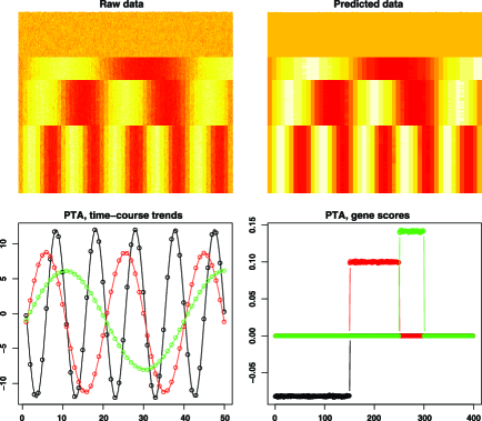
Second, we study how the performance of the proposed method changes when the number of subjects increases. In real applications, the number of subjects varies a lot. For instance, the circadian rhythm data set that we consider in Section 4 has 3 subjects, while the burn patient data set we consider in Section 5 has 28 subjects. Thus, we want to investigate the performance of PTA when the number of subjects changes. We run the simulations with different numbers of subjects. The design of the simulation is shown in Table 2. We change the number of subjects from 1 to 40 with the number of features, the number of noisy features and the number of time points fixed. The error term is drawn from $N(0,0.1)$. For each case, we repeat the simulation 10 times. One can see that as the number of subjects increases, the performance of our method improves on both the percentage of explained variance and the accuracy of detecting informative features. We plot one example as shown in Figure 2. The top-left heatmap shows the raw data. The top-right heatmap shows the prediction of PTA. The bottom 250 genes of the heatmap reflect three time-course patterns with noise filtered. The remaining genes of the heatmap have zero values because noise has been filtered. The bottom-left panel of Figure 2 shows PTs identified by PTA. We can see that the first PT successfully extracts the dominant frequency belonging to the first 200 genes; the second PT extracts the second dominant frequency belonging to the second 100 genes; the third PT extracts the third dominant frequency belonging to the remaining 50 genes. We also plot the scores in the right-bottom panel of Figure 2, which reflect the contributions of each gene on the time-course patterns. In the first PT, the first 150 features have nonzero scores, while the remaining features have zero scores. In the second PT, the features from 151 to 250 have nonzero features, but the remaining features have zero scores. In the third PT, the features from 251 to 300 have nonzero features, while the remaining features have zero scores. The results demonstrate that our PTA method works well on the data set with multiple time-course patterns and noisy genes. Under the designed model (3) and parameters in Table 2, PTA shows good performance even with a small sample size.

Figure 2: One example in design 2. PTA on the simulated data with multiple patterns and noisy genes. Data was simulated according to (3) with $\epsilon_{\mathit{npt}}\sim N(0,0.1)$, $P=400$, $N=10$ and $T=50$. The top-left panel shows the simulated raw data, with rows indicating genes, columns indicating samples ordered by time points and samples from the same time point grouped together. The top-right panel shows the predicted data with three time-course trends. The bottom-left panel shows top three PTs of PTA with three types of frequencies: black, the first PT which extracts the dominant frequency $f_{1}=1$; red, the second PT which extracts the second dominant frequency $f_{2}=0.5$; green, the third PT which extracts the third dominant frequency $f_{3}=0.25$. The bottom-right panel shows scores of PTA on the simulated time-course gene expression data with three types of frequencies: black, the first PT; red, the second PT; green, the third PT. Tuning parameters are obtained by tenfold cross-validation.

Third, we study the relationship between the performance of PTA and the signal-to-noise ratio. Genomic technologies such as Microarray and RNA-seq have measurement errors. It affects the detection of true signals in real data sets. It is necessary to investigate the performance of PTA with different levels of signal-to-noise ratio. We fix the number of features, the number of noninformative features, the number of subjects and the number of time points, while increasing the noise variance in (3) from 0.1 to 4 as shown in Table 3. Based on the simulation

Table 3: Design 3: studying the relationship between the performance of PTA and the signal-to-noise ratio. Simulations are performed according to (3)

Case	$\bolds{P}$	$\bolds{\mathcal{P}}$	$\bolds{N}$	$\bolds{T}$	$\bolds{\epsilon_{\mathit{npt}}}$	SNR	Nonzero features	Explained variance
1	400	300	1	50	$N(0,0.1)$	7.07	(150.0, 101.4, 50.4) $\pm$ (0.00, 1.51, 0.97)	0.838 $\pm$ 0.0005
2	400	300	1	50	$N(0,0.2)$	3.54	(150.6, 100.8, 50.5) $\pm$ (0.84, 1.14, 0.71)	0.778 $\pm$ 0.0007
3	400	300	1	50	$N(0,0.35)$	2.02	(151.2, 101.0, 50.3) $\pm$ (2.04, 1.41, 0.95)	0.649 $\pm$ 0.0021
4	400	300	1	50	$N(0,0.7)$	1.01	(149.7, 100.0, 49.9) $\pm$ (1.42, 2.62, 3.60)	0.374 $\pm$ 0.0030
5	400	300	1	50	$N(0,1)$	0.71	(147.7, 98.0, 47.7) $\pm$ (3.97, 3.33, 3.06)	0.230 $\pm$ 0.0057
6	400	300	1	50	$N(0,2)$	0.35	(145.9, 95.5, 45.0) $\pm$ (2.23, 1.58, 0.00)	0.081 $\pm$ 0.0031
7	400	300	1	50	$N(0,4)$	0.18	(145.0, 95.0, 45.0) $\pm$ (0.00, 0.00, 0.00)	0.047 $\pm$ 0.0013

(3), we calculate the signal-to-noise ratio $\mathrm{SNR}=\frac{1}{\sqrt{2}\sigma_{\epsilon}}$. One can see that the larger the signal-to-noise ratio is, the more accurate the detected informative features are. Also, the larger the signal-to-noise ratio is, the larger the percentage of explained variance is. Even when the signal-to-noise ratio is small, for example, 0.18, PTA still has good estimation of informative features which are close to the true values.

Table 4: Design 4: studying the performance of PTA with the presence of “noisy subjects”. Simulations are performed according to (3)

Case	$\bolds{P}$	$\bolds{\mathcal{P}}$	$\bolds{N}$	$\bolds{T}$	$\bolds{\mathcal{N}}$	$\bolds{\mathcal{N}/N}$	Nonzero features	Explained variance
1	400	300	50	50	$5$	0.1	(150.0, 100.3, 50.0) $\pm$ (0.00, 0.95, 0.00)	0.869 $\pm$ 0.0001
2	400	300	50	50	$10$	0.2	(150.0, 100.5, 50.0) $\pm$ (0.00, 1.08, 0.00)	0.768 $\pm$ 0.0001
3	400	300	50	50	$15$	0.3	(150.0, 100.0, 50.0) $\pm$ (0.00, 0.00, 0.00)	0.668 $\pm$ 0.0002
4	400	300	50	50	$20$	0.4	(150.0, 100.5, 50.0) $\pm$ (0.00, 1.58, 0.00)	0.568 $\pm$ 0.0002

Fourth, we study the effect of “noisy subjects” on the performance of the method. In real data sets, some subjects can be “outliers.” It may be due to the existence of unknown subpopulations or experimental errors. We design simulations with the presence of “noisy subjects” as illustrated in Table 4. We fix the total number of subjects $N$ as 50, and increase the number of “noisy subjects”, which is denoted by $\mathcal{N}$. In this design, we assume the error term in (3) follows a normal distribution, which is $\epsilon_{\mathit{npt}}\sim N(0,0.1)$. We repeat the simulation 10 times. One can see that from Table 4, the ability of detecting informative features is robust against the percentage of “noisy subjects”, though the percentage of explained variance decreases when the percentage of “noisy subjects” increases.

Fifth, we study the performance of PTA in terms of less number of time points and larger number of features. Once a biological sample is collected, on one hand, the lab technician may label it at once so that thousands of genes can be scanned simultaneously. While on the other hand, it is very time and labor intensive to extract samples at many time points. Thus, we want to investigate the performance of PTA where there are a larger number of features and a smaller number of time points. We design the simulation as shown in Table 5. We reduce the number of time points to 20 and 10, respectively, and increase the number of features to 1000 and 10,000, respectively. We simulate data based on (3) with $\epsilon_{\mathit{npt}}\sim N(0,0.1)$. We repeat the simulation 10 times. The average performance of PTA under each setting is shown in Table 5. One can see even with a smaller number of time points and a larger number of features, PTA can still do a good job. Nevertheless, increasing the number of time points and reducing the number of noisy features help the performance of PTA.

Table 5: Design 5: studying the performance of PTA in terms of a smaller number of time points and a larger number of features. Simulations are performed according to (3)

Case	$\bolds{P}$	$\bolds{N}$	$\bolds{T}$	Nonzero features	Explained variance
1	00,400	1	20	$(150.9,100.3,50.5)\pm(1.37,0.95,1.18)$	0.810 $\pm$ 0.0008
2	00,400	1	10	$(150.0,101.6,50.0)\pm(3.27,3.20,3.16)$	0.730 $\pm$ 0.0026
3	0,1000	1	20	$(151.5,101.0,50.1)\pm(1.51,1.41,0.32)$	0.776 $\pm$ 0.0007
4	0,1000	1	10	$(148.5,96.9,49.1)\pm(2.84,2.81,3.81)$	0.688 $\pm$ 0.0019
5	10,000	1	20	$(151.7,100.0,49.7)\pm(1.70,0.00,1.70)$	0.473 $\pm$ 0.0006
6	10,000	1	10	$(148.0,98.6,47.6)\pm(3.20,3.27,3.37)$	0.370 $\pm$ 0.0017

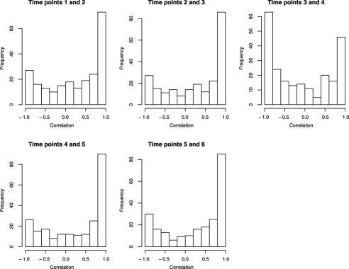
We have been assuming the error term $\epsilon_{\mathit{npt}}$ follows a normal distribution so far. However, we want to know how much the method is affected if the noise term $\epsilon_{\mathit{npt}}$ has some serial correlation within observations from the same subject. The circadian rhythm data set that we consider in Section 4 shows evidence of such correlation. As shown in Figure 3, many genes have high time-series correlation. We use the model of (3) but generate $\epsilon_{\mathit{npt}}$ from the first order auto-regression model with correlation $\rho=\operatorname{corr}(\epsilon_{\mathit{npt}},\epsilon_{np(t+1)})$, denoted by $\operatorname{AR}(1,\rho)$. The design is illustrated in Table 5. We study the performance of PTA with respect to different levels of “noisy features”, different numbers of subjects and different correlation levels in the error term. The results are shown in Table 6. One can see that PTA has good performance in terms of serial correlation. PTA is robust against the percentage of noninformative features with the number of subjects, the number of time points and the error term held fixed. PTA achieves a good performance even with a small number of subjects under the condition that the noise term has time-series correlation. Overall, the performance of PTA is robust against serial correlation. Nevertheless, PTA has better performance when the noise term has smaller serial correlation.

Figure 3: Time-series correlation in noise in the circadian rhythm data set in Section 4. Histograms of values for correlation between adjacent time points for 288 genes.

The three components of the time signal are orthogonal functions in (3). We want to know what happens if the latent time patterns are “correlated”. For instance, the expression of some genes may decay or increase with time but with different rates and perhaps oscillatory behavior. The principal trends from the burn data set that we consider in Section 5 are an example of such correlations among latent time course patterns. We design the following experiment. Let $\mathbf{Y}$ indicate longitudinal high-throughput gene expression from $P$ genes, $N$ subjects and $T$ time points. We assign the values of elements in $\mathbf{Y}$ as follows:

$$y_{\mathit{npt}}=\sin(0.5\cdot\pi\cdot t)\cdot\sum_{k=0}^{2}w_{k,p}\cdot\exp(\xi_{k}t)+\epsilon_{\mathit{npt}},$$ (10)

where $\xi_{0}<0$, $\xi_{1}<0$, $\xi_{2}<0$, $p$ is the gene, $n$ is the subject, $t$ is time, $\epsilon_{\mathit{npt}}$ is the error term, $w_{0,p}$ is $I(0<p\leq 150)$, $w_{1,p}$ is $I(150<p\leq 250)$, $w_{2,p}$ is $I(250<p\leq 300)$ and $I$ denotes the indicator function. We set $\xi_{0}=-1$, $\xi_{1}=-2$, $\xi_{2}=-3$ in the simulation. We assume that the error term follows a normal distribution $N(0,0.1)$ as shown in Table 6. We repeat the simulation 10 times. One can see that PTA

= Case $\bolds{P}$ $\bolds{\mathcal{P}}$ $\bolds{N}$ $\bolds{T}$ $\bolds{\mathcal{P}/{P}}$ $\bolds{\epsilon_{\mathit{npt}}}$ Nonzero features Explained variance 1 $400$ 100 $1$ 50 0.25 $\operatorname{AR}(1)$, $\rho=0.8$ (150.4, 101.2, 51.0) $\pm$ (0.97, 1.40, 1.70) 0.812 $\pm$ 0.0017 2 $500$ 200 $1$ 50 0.40 $\operatorname{AR}(1)$, $\rho=0.8$ (150.2, 100.0, 50.0) $\pm$ (0.42, 0.00, 0.00) 0.800 $\pm$ 0.0024 3 $600$ 300 $1$ 50 0.50 $\operatorname{AR}(1)$, $\rho=0.8$ (150.3, 100.5, 50.1) $\pm$ (0.67, 0.85, 0.32) 0.788 $\pm$ 0.0017 4 $1000$ 700 $1$ 50 0.70 $\operatorname{AR}(1)$, $\rho=0.8$ (150.6, 101.6, 51.5) $\pm$ (1.07, 1.96, 2.12) 0.745 $\pm$ 0.0014 5 $400$ 100 $5$ 50 0.25 $\operatorname{AR}(1)$, $\rho=0.8$ (150.0, 100.4, 50.7) $\pm$ (0.00, 0.97, 1.49) 0.900 $\pm$ 0.0007 6 $400$ 100 $10$ 50 0.25 $\operatorname{AR}(1)$, $\rho=0.8$ (150.4, 100.1, 50.0) $\pm$ (1.26, 0.32, 0.00) 0.914 $\pm$ 0.0004 7 $400$ 100 $40$ 50 0.25 $\operatorname{AR}(1)$, $\rho=0.8$ (150.0, 100.7, 50.1) $\pm$ (0.00, 1.64, 0.32) 0.925 $\pm$ 0.0001 8 $400$ 100 $1$ 50 0.25 $\operatorname{AR}(1)$, $\rho=0.1$ (150.0, 100.8, 50.2) $\pm$ (0.00, 1.23, 0.63) 0.838 $\pm$ 0.0003 9 $400$ 100 $1$ 50 0.25 $\operatorname{AR}(1)$, $\rho=0.5$ (150.1, 100.8, 50.6) $\pm$ (0.32, 1.03, 1.26) 0.833 $\pm$ 0.0003

Table 6: Design 6: studying the performance of PTA when the noise term has time series correlation. Simulations are performed according to (3)

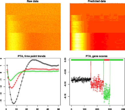
works when underlying patterns are correlated. We plot one example which is shown in Figure 4. This example shows that PTA can also detect the true informative features and extract the true patterns. Besides, increasing the number of samples helps the performance of PTA as shown in Table 7. Comparing Table 7 with Tables 1 and 2, one can see that PTA achieves better performance when the underlying time-course patterns are less correlated.

Figure 4: One example in design 6. PTA on the simulated data with multiple correlated patterns and noisy genes. Data was simulated according to (10) with $\epsilon_{\mathit{npt}}\sim N(0,0.1)$, $P=400$, $N=10$ and $T=50$. The top-left panel shows the simulated raw data, with rows indicating genes, columns indicating samples ordered by time points and samples from the same time point grouped together. The top-right panel shows the predicted data with three PTs. The bottom-left panel shows the identified top three PTs by PTA: black, the first PT which extracts the dominant pattern $\exp(-t)\cdot\sin(0.5\cdot\pi\cdot t)$; red, the second PT which extracts the second dominant pattern $\exp(-2t)\cdot\sin(0.5\cdot\pi\cdot t)$; green, the third PT which extracts the third dominant pattern $\exp(-3t)\cdot\sin(0.5\cdot\pi\cdot t)$. The bottom-right panel shows scores of genes for their contributions to the top three PTs: black, the first PT; red, the second PT; green, the third PT. Tuning parameters are obtained by tenfold cross-validation.

Table 7: Design 7: studying the performance of PTA when the underlying time-course patterns are correlated. Simulations are performed according to (10)

Case	$\bolds{P}$	$\bolds{\mathcal{P}}$	$\bolds{N}$	$\bolds{T}$	$\bolds{\epsilon_{\mathit{npt}}}$	Nonzero features	Explained variance
1	$400$	100	$1$	50	$N(0,0.1)$	(153.0, 97.9, 45.2) $\pm$ (2.21, 3.28, 0.63)	0.530 $\pm$ 0.0088
2	$500$	200	$1$	50	$N(0,0.1)$	(151.1, 96.9, 45.0) $\pm$ (3.38, 2.88, 0.00)	0.477 $\pm$ 0.0125
3	$600$	300	$1$	50	$N(0,0.1)$	(151.9, 97.0, 46.9) $\pm$ (3.41, 2.62, 3.25)	0.432 $\pm$ 0.0086
4	$1000$	700	$1$	50	$N(0,0.1)$	(151.7, 96.9, 45.2) $\pm$ (2.45, 3.07, 0.63)	0.315 $\pm$ 0.0078
5	$400$	100	$5$	50	$N(0,0.1)$	(152.3, 102.1, 50.2) $\pm$ (2.11, 2.13, 3.26)	0.543 $\pm$ 0.0042
6	$400$	100	$10$	50	$N(0,0.1)$	(150.8, 103.0, 50.0) $\pm$ (1.48, 1.56, 0.82)	0.550 $\pm$ 0.0013
7	$400$	100	$40$	50	$N(0,0.1)$	(150.1, 100.7, 50.0) $\pm$ (0.32, 1.64, 0.00)	0.551 $\pm$ 0.0007

Finally, we show why we need the penalty for smoothing in the model (2) instead of using the Penalized Matrix Analysis [PMA; cf. Witten, Tibshirani and Hastie (2009)]. To compare the performance of PTA and PMA in extracting time-course patterns of gene expression with noisy genes, we simulate a gene expression data set consisting of genes with time-course patterns and noisy genes. Let $\mathbf{Y}=(y_{pt})$ be a gene expression matrix with 100 genes and 30 time points. Elements of matrix $Y$ are simulated according to the following model:

$$y_{pt}=\cases{\cos(0.6t)+\varepsilon_{pt},&\quad$p\leq 70$,\cr\varepsilon_{pt},&\quad$p>71$,}$$ (11)

where $p$ is the indicator of gene, $t$ is time and $\varepsilon_{pt}\sim N(0,1)$. The heatmap of simulated raw gene expression is plotted in the top-left panel of Figure 5. Rows show genes and columns indicate time points. The simulated data are represented in the top-left panel of Figure 5. The true time-course pattern is

Figure 5: Comparison of PTA and PMA. Data is simulated according to procedure in (11). The top-left panel shows the simulated raw data, with rows indicating genes and columns indicating samples ordered by time points. The top-right panel shows the true signal. The bottom-left panel shows the predicted data using PTA. The bottom-right panel shows the predicted data using PMA.

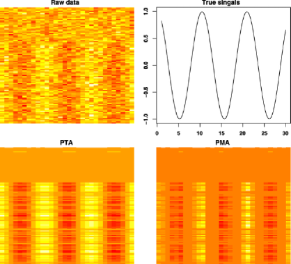
illustrated in the top-right panel of Figure 5, which is the $\cos(0.6t)$ curve. We applied PTA and PMA on this simulated data using single component decomposition. The prediction of PTA is obtained by $\hat{\mathbf{a}}\hat{\bolds{\theta}}\mathbf{B}^{\mathsf{T}}$, and presented by a heatmap in the bottom-left panel of Figure 5. The prediction of PMA is obtained by $\hat{d}\hat{\mathbf{u}}\hat{\mathbf{v}}^{\mathsf{T}}$, where $\{\hat{\mathbf{u}},\hat{\mathbf{v}}\}=\arg\max_{\mathbf{u},\mathbf{v}}\mathbf{u}^{\mathsf{T}}\mathbf{Y}\mathbf{v}$, subject to $\|\mathbf{u}\|_{1}\leq c_{1}$, $\|\mathbf{u}\|^{2}_{2}=1$, $\|\mathbf{v}\|_{1}\leq c_{2}$, $\|\mathbf{v}\|_{2}^{2}=1$, $\hat{d}=\hat{\mathbf{u}}^{\mathsf{T}}\mathbf{Y}\hat{\mathbf{v}}$. The

Figure 6: Comparison of time-course patterns and scores identified by PTA and PMA on the simulated data based on (11). The top-left panel shows the principal trend identified by PTA. Top-right panel shows the gene scores of PTA. The bottom-left panel shows the time-course pattern identified by PMA. The bottom-right panel shows the gene scores of PMA.

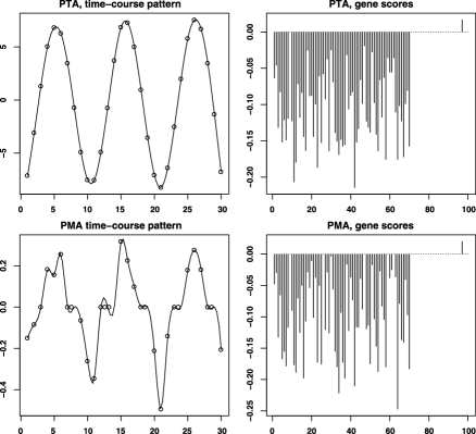
prediction of PMA is presented by a heatmap in the bottom-right panel of Figure 5. One can see that the prediction of PTA extracts a clear cosine pattern, while the prediction of PMA is a segmented curve. We also plot the time-course patterns and scores of genes which are identified by PTA and PMA, respectively, in Figure 6. Overall, the results suggest that PTA has better performance than PMA in extracting time-course patterns of gene expressions.

4 Circadian rhythm gene expression data

Circadian rhythms are biological processes that display endogenous and entrainable oscillation of about 24 hours. These rhythms are driven by a circadian clock. Circadian rhythms have been widely observed in live organisms, including plants, animals, fungi and cyanobacteria. Circadian regulations play important roles to maintain normal living of live organisms. In particular, disruption to rhythms in humans may result in a number of disorders, for example, bipolar disorder and sleep disorders, and in the longer term is believed to have significant adverse health consequences on peripheral organs outside the brain, particularly in the development or exacerbation of cardiovascular disease. Thus, circadian regulatory systems have attracted a lot of attention for research and provide a good example to validate our PTA approach. Here, to validate PTA, we use a circadian rhythm gene expression data set from a well-studied pattern organism—arabidopsis thaliana rosette.

Bläsing et al. (2005) generated time-course gene expression data from arabidopsis thaliana rosettes in a light-dark treatment experiment. ATH1 arrays (Affymetrix Arabidopsis ATH1 Genome Array, www.affymetrix.com) were used to measure gene expression to study how diurnal cycle affects gene expression of arabidopsis thaliana rosettes. Arabidopsis thaliana rosettes were harvested six times during 12-h-light/12-h-dark treatments. Three replicate samples were collected 4, 8 and 12 hours into the light period and 4, 8 and 12 hours into the night. The time points were presented by 4, 8, 12, 16, 20, 24 h. Gene expression data were preprocessed by MAS [MicroArray Suite Software; Hubbell, Liu and Mei (2002)] to evaluate probe set signals of the array. The generated data files were further processed by RMA (Robust Multi-array Average, from R-package Affy, http://www.bioconductor.org) to normalize and estimate signal intensities. Gene expression values were centered with mean 0. We preselected 228 genes with known circadian regulation functions. This data set contains 228 genes, 6 time points and 3 replicates. Thus, to analyze circadian gene expression pattern according to time, the standard PCA cannot be applied while PTA should be used. We solve the following optimization problem to extract the underlying time-course gene expression patterns by PTA:

$$\min_{\mathbf{A},\bolds{\Theta}}L(\mathbf{A},\bolds{\Theta}|\mathbf{Y})\quad\mbox{such that}\quad\bolds{\Theta}\bolds{\Omega}\bolds{\Theta}^{\mathsf{T}}\leq c_{1}\quad\mbox{and}\quad\|\mathbf{A}\|_{2}=1.$$

We plot the variance of each component in the left panel of Figure 7. One can see that the first two PTs occupy much larger variance than the rest of components. We also plot the first three PTs in the right panel of Figure 7. From the picture, one can see that the first two PTs extract the patterns with greatest longitudinal variations, which is consistent with the results in the left panel of Figure 7. In particular, the first cosine shape pattern is the dominant shape, which agrees with the time pattern of light in the experiment. For the first PT, 96 of the total 228 genes

Figure 7: PTA for the gene expression of genes with known circadian regulated functions in Arabidopsis thaliana rosette. The left panel shows variances for each component. Each bar shows one component, ordered by the rank of component. The height of each bar shows the variance for each component. The right panel shows the top three PTs. Black indicates the first PT. Red indicates the second PT. Green indicates the third PT.

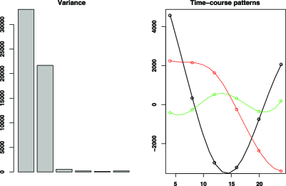
have positive weights, while 132 of them have negative weights. Those genes with positive weights share the same up and down directions with the principal trend, while those with negative weights share the opposite up and down directions. For example, the gene CAT2 with a positive weight has a peak at the fourth hour. An independent experiment has revealed the CAT2 mRNA accumulated to a peak four hours after the onset of illumination and then declined, when etiolated seedlings were illuminated [Zhong et al. (1994)]. Our principal trend analysis suggests that light can be depicted as an activator of CAT2 gene expression, probably through the action of the phytochrome sensory system. The circadian clock could be envisaged as a permissive regulator with respect to light, allowing induction of CAT2 at dawn.

5 Gene expression of a burn cohort

Despite ongoing improvements in resuscitation, care and outcomes, burn injury remains a significant health and economic burden globally. The current approach to the clinical management of these patients remains limited by insufficient understanding of the pathobiology of the disease. To describe the human genomic response to burns, a cohort of burn patients were monitored and their gene expression was measured at multiple time points (www.gluegrant.org). The longitudinal data can be divided into three stages—early stage (within one day to ten days with three days median time), middle stage (eleven days to fourty-nine days with nineteen days median time) and late stage (fifty days to more than one year). Blood samples of burn patients were collected to measure the gene expression by the Affymetrix HU133 Plus 2.0 arrays [Zhang, Tibshirani and Davis (2010, 2013)]. Each array consisted of 54,675 probe sets. Gene expression data was normalized by dChip [see Li and Wong (2001)] and further reduced to 1000 probe sets with the top 1000 highest coefficient of variation (CV, standard deviation/mean). We take 28 surviving patients with multiple-organ-failure scores (MOF) of three or less. Clinically, they belong to the “uncomplicated group.”

In this study, a preknown set of burn-related genes is not available. An important task is to automatically identify the subset of genes involved in burn response and extract their time-course expression patterns. As suggested in the last simulation of Section 3, not PMA in Witten, Tibshirani and Hastie (2009), but PTA is suitable for dimension-reduction and feature selection in the time-course gene expression data in a population of patients. Thus, we solve the following optimization problem:

$$\min_{\mathbf{A},\bolds{\Theta}}L(\mathbf{A},\bolds{\Theta}|\mathbf{Y})\quad\mbox{such that}\quad\bolds{\Theta}\bolds{\Omega}\bolds{\Theta}^{\mathsf{T}}\leq c_{1},\qquad\|\mathbf{A}\|_{1}\leq c_{2}\quad\mbox{and}\quad\|\mathbf{A}\|_{2}=1.$$

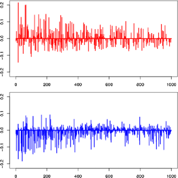
After applying PTA on this data set of burn patients, we investigate the extracted PTs and identified genes that have nonzero scores. The top two PTs are shown in Figure 8, and the scores of genes

Figure 8: PTA on burn data. Left: the first PT; right: the second PT.

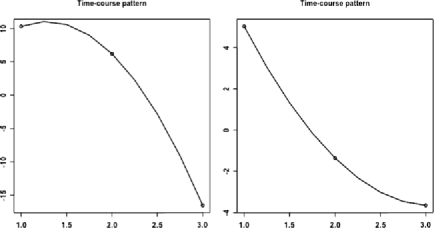
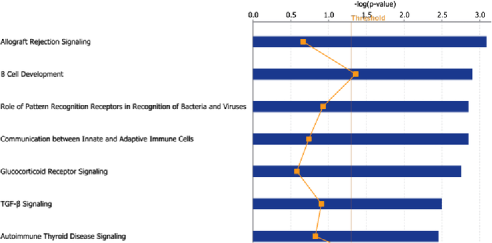
are shown in Figure 9. There are 400 genes with contributions on the first PT, and 600 genes with contributions on the second PT. We applied the enrichment analysis (Fisher’s exact test)

Figure 9: PTA on burn data. The scores of genes for the first two PTs are shown. The upper panel: the first PT; the lower panel: the second PT.

using the Ingenuity Pathway Analysis (IPA) tool (http://www.ingenuity.com/) on the genes with nonzero scores for the first and second PTs, respectively. Top enriched canonical pathways are shown in Figures 10 and 11. Genes in the

Figure 10: PTA on burn data. Enriched canonical pathways for genes with nonzero scores at the first PT.

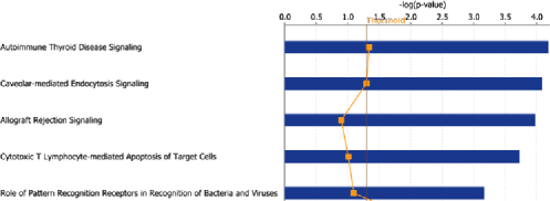
first PT have functions related to inflammatory responses, immune cell trafficking, and cell-to-cell signaling and interaction functions. Genes in the second PT have functions related to allograft rejection signaling, B cell development, pattern recognition receptors in recognition of bacteria and viruses, communication between innate and adaptive immune cells, and cellular movement, growth and proliferation functions. PTA provides an overview of the dynamics of genomic response to burn injuries and extracts genes for further investigation to better

Figure 11: PTA on burn data. Enriched canonical pathways for genes with nonzero scores at the second PT.

understand the pathobiology of burn disease. For example, gene IFIT1 is one of the identified genes with nonzero scores in the first PT. It has been shown that in mammalian cells, it is synthesized in response to viral infection, and consequently assigns resistive activity against viral invasion to cells [Li et al. (2010)]. It is common for burn patients to suffer from infectious episodes, which are caused by viruses [Finnerty et al. (2006)]. Thus, PTA successfully identified the key regulatory element IFIT1, which plays an important role for the recovery of burn patients. Overall, PTA characterizes the inflammatory transcriptome following a burn injury and identifies the burn-induced immuno-inflammatory dysfunction and hyperinflammatory response. Comprehensive understanding of the molecular mechanisms of burn disease will ultimately lead to novel and profound advancements in clinical care.

6 Discussion

By virtue of matrix theory, PCA is an important methodology to study data structure. It has been widely used to analyze clinical and biological data. Combining the lasso technique with matrix decomposition, the regularized PCA method can be applied to high-throughput genomic or proteomic data. In the case of a time-course experimental scenario, such data sets have four dimensions (feature, sample, time, gene/protein expression), traditional PCA or regularized PCA cannot be used directly. We have developed a new principal trend analysis (PTA) method for time-course data modeling. PTA incorporates smoothing techniques for time and sparsity techniques for genes when it is necessary. Our simulations and applications on real data sets show that PTA works well and outperforms regularized PCA (PMA) on time-course gene expression data.

The proposed PTA focuses on a population’s time-course patterns. However, it also works when the number of subjects equals one. If subjects are too diverse and cannot be treated as one population, we can apply PTA on each subject and identify personalized longitudinal gene expression patterns and important genes.

In clinical and biological studies, people may collect different types of data sets on the same patients or samples at multiple time points. Those time-course data includes gene expression and protein abundance, and clinical measurements of the same patients, etc. It will be interesting to extract the associated relationships among features from multiple longitudinal data sets. Developing methods to handle such tasks will be an important future work.

References

- Bläsing et al. (2005) {barticle}[author] \bauthor\bsnmBläsing, \bfnmO. E.\binitsO. E., \bauthor\bsnmGibon, \bfnmY.\binitsY., \bauthor\bsnmGünther, \bfnmM.\binitsM., \bauthor\bsnmHöhne, \bfnmM.\binitsM., \bauthor\bsnmMorcuende, \bfnmR.\binitsR., \bauthor\bsnmOsuna, \bfnmD.\binitsD., \bauthor\bsnmThimm, \bfnmO.\binitsO., \bauthor\bsnmUsadel, \bfnmB.\binitsB., \bauthor\bsnmScheible, \bfnmW. R.\binitsW. R. and \bauthor\bsnmStitt, \bfnmM.\binitsM. (\byear2005). \btitleSugars and circadian regulation make major contributions to the global regulation of diurnal gene expression in Arabidopsis. \bjournalThe Plant Cell Online \bvolume17 \bpages3257. \bptokimsref \endbibitem
- Boyd and Vandenberghe (2004) {bbook}[mr] \bauthor\bsnmBoyd, \bfnmStephen\binitsS. and \bauthor\bsnmVandenberghe, \bfnmLieven\binitsL. (\byear2004). \btitleConvex Optimization. \bpublisherCambridge Univ. Press, \blocationCambridge. \bidmr=2061575 \bptokimsref \endbibitem
- Breiman and Spector (1992) {barticle}[author] \bauthor\bsnmBreiman, \bfnmL.\binitsL. and \bauthor\bsnmSpector, \bfnmP.\binitsP. (\byear1992). \btitleSubmodel selection and evaluation in regression. The -random case. \bjournalInternational Statistical Review \bvolume60 \bpages291–319. \bptokimsref \endbibitem
- De Leeuw and Michailidis (1994) {binproceedings}[author] \bauthor\bsnmDe Leeuw, \bfnmJ.\binitsJ. and \bauthor\bsnmMichailidis, \bfnmG.\binitsG. (\byear1994). \btitleBlock relaxation algorithms in statistics. In \bbooktitleInformation Systems and Data Analysis \bpages308–325. \bpublisherSpringer, \blocationBerlin. \bptokimsref \endbibitem
- Finnerty et al. (2006) {barticle}[author] \bauthor\bsnmFinnerty, \bfnmC. C.\binitsC. C., \bauthor\bsnmHerndon, \bfnmD. N.\binitsD. N., \bauthor\bsnmPrzkora, \bfnmR.\binitsR., \bauthor\bsnmPereira, \bfnmC. T.\binitsC. T., \bauthor\bsnmOliveira, \bfnmH. M.\binitsH. M., \bauthor\bsnmQueiroz, \bfnmD. M. M.\binitsD. M. M., \bauthor\bsnmRocha, \bfnmA. M. C.\binitsA. M. C. and \bauthor\bsnmJeschke, \bfnmM. G.\binitsM. G. (\byear2006). \btitleCytokine expression profile over time in severely burned pediatric patients. \bjournalShock \bvolume26 \bpages13–19. \bptokimsref \endbibitem
- Hastie, Tibshirani and Friedman (2009) {bbook}[mr] \bauthor\bsnmHastie, \bfnmTrevor\binitsT., \bauthor\bsnmTibshirani, \bfnmRobert\binitsR. and \bauthor\bsnmFriedman, \bfnmJerome\binitsJ. (\byear2009). \btitleThe Elements of Statistical Learning: Data Mining, Inference, and Prediction, \bedition2nd ed. \bpublisherSpringer, \blocationNew York. \biddoi=10.1007/978-0-387-84858-7, mr=2722294 \bptokimsref \endbibitem
- Hubbell, Liu and Mei (2002) {barticle}[pbm] \bauthor\bsnmHubbell, \bfnmEarl\binitsE., \bauthor\bsnmLiu, \bfnmWei-Min\binitsW.-M. and \bauthor\bsnmMei, \bfnmRui\binitsR. (\byear2002). \btitleRobust estimators for expression analysis. \bjournalBioinformatics \bvolume18 \bpages1585–1592. \bidissn=1367-4803, pmid=12490442 \bptokimsref \endbibitem
- Kimeldorf and Wahba (1970) {barticle}[mr] \bauthor\bsnmKimeldorf, \bfnmGeorge S.\binitsG. S. and \bauthor\bsnmWahba, \bfnmGrace\binitsG. (\byear1970). \btitleA correspondence between Bayesian estimation on stochastic processes and smoothing by splines. \bjournalAnn. Math. Statist. \bvolume41 \bpages495–502. \bidissn=0003-4851, mr=0254999 \bptokimsref \endbibitem
- Kohavi (1995) {binproceedings}[author] \bauthor\bsnmKohavi, \bfnmR.\binitsR. (\byear1995). \btitleA study of cross-validation and bootstrap for accuracy estimation and model selection. In \bbooktitleInternational Joint Conference on Artificial Intelligence, Vol. 14 \bpages1137–1145. \bpublisherLawrence Erlbaum Associates, \blocationMahwah, NJ. \bptokimsref \endbibitem
- Li and Wong (2001) {barticle}[pbm] \bauthor\bsnmLi, \bfnmC.\binitsC. and \bauthor\bsnmWong, \bfnmW. H.\binitsW. H. (\byear2001). \btitleModel-based analysis of oligonucleotide arrays: Expression index computation and outlier detection. \bjournalProc. Natl. Acad. Sci. USA \bvolume98 \bpages31–36. \biddoi=10.1073/pnas.011404098, issn=0027-8424, pii=011404098, pmcid=14539, pmid=11134512 \bptokimsref \endbibitem
- Li et al. (2010) {barticle}[author] \bauthor\bsnmLi, \bfnmH. T.\binitsH. T., \bauthor\bsnmSu, \bfnmY. P.\binitsY. P., \bauthor\bsnmCheng, \bfnmT. M.\binitsT. M., \bauthor\bsnmXu, \bfnmJ. M.\binitsJ. M., \bauthor\bsnmLiao, \bfnmJ.\binitsJ., \bauthor\bsnmChen, \bfnmJ. C.\binitsJ. C., \bauthor\bsnmJi, \bfnmC. Y.\binitsC. Y., \bauthor\bsnmAi, \bfnmG. P.\binitsG. P. and \bauthor\bsnmWang, \bfnmJ. P.\binitsJ. P. (\byear2010). \btitleThe interaction between interferon-induced protein with tetratricopeptide repeats-1 and eukaryotic elongation factor-1A. \bjournalMolecular and Cellular Biochemistry \bvolume337 \bpages101–110. \bptokimsref \endbibitem
- Mairal et al. (2010) {barticle}[mr] \bauthor\bsnmMairal, \bfnmJulien\binitsJ., \bauthor\bsnmBach, \bfnmFrancis\binitsF., \bauthor\bsnmPonce, \bfnmJean\binitsJ. and \bauthor\bsnmSapiro, \bfnmGuillermo\binitsG. (\byear2010). \btitleOnline learning for matrix factorization and sparse coding. \bjournalJ. Mach. Learn. Res. \bvolume11 \bpages19–60. \bidissn=1532-4435, mr=2591620 \bptokimsref \endbibitem
- Tibshirani (1996) {barticle}[mr] \bauthor\bsnmTibshirani, \bfnmRobert\binitsR. (\byear1996). \btitleRegression shrinkage and selection via the lasso. \bjournalJ. R. Stat. Soc. Ser. B Stat. Methodol. \bvolume58 \bpages267–288. \bidissn=0035-9246, mr=1379242 \bptokimsref \endbibitem
- Wahba (1990) {bbook}[mr] \bauthor\bsnmWahba, \bfnmGrace\binitsG. (\byear1990). \btitleSpline Models for Observational Data. \bseriesCBMS-NSF Regional Conference Series in Applied Mathematics \bvolume59. \bpublisherSIAM, \blocationPhiladelphia, PA. \biddoi=10.1137/1.9781611970128, mr=1045442 \bptokimsref \endbibitem
- Witten and Tibshirani (2009) {barticle}[mr] \bauthor\bsnmWitten, \bfnmDaniela M.\binitsD. M. and \bauthor\bsnmTibshirani, \bfnmRobert J.\binitsR. J. (\byear2009). \btitleExtensions of sparse canonical correlation analysis with applications to genomic data. \bjournalStat. Appl. Genet. Mol. Biol. \bvolume8 \bpagesArt. 28, 29. \biddoi=10.2202/1544-6115.1470, issn=1544-6115, mr=2533636 \bptokimsref \endbibitem
- Witten, Tibshirani and Hastie (2009) {barticle}[pbm] \bauthor\bsnmWitten, \bfnmDaniela M.\binitsD. M., \bauthor\bsnmTibshirani, \bfnmRobert\binitsR. and \bauthor\bsnmHastie, \bfnmTrevor\binitsT. (\byear2009). \btitleA penalized matrix decomposition, with applications to sparse principal components and canonical correlation analysis. \bjournalBiostatistics \bvolume10 \bpages515–534. \biddoi=10.1093/biostatistics/kxp008, issn=1468-4357, pii=kxp008, pmcid=2697346, pmid=19377034 \bptokimsref \endbibitem
- Zhang and Davis (2013) {bmisc}[mr] \bauthor\bsnmZhang, \bfnmY.\binitsY. and \bauthor\bsnmDavis, \bfnmR.\binitsR. (\byear2013). \bhowpublishedSupplement to “Principal trend analysis for time-course data with applications in genomic medicine.” DOI:\doiurl10.1214/13-AOAS659SUPP. \bptokimsref \endbibitem
- Zhang, Tibshirani and Davis (2010) {barticle}[mr] \bauthor\bsnmZhang, \bfnmYuping\binitsY., \bauthor\bsnmTibshirani, \bfnmRobert J.\binitsR. J. and \bauthor\bsnmDavis, \bfnmRonald W.\binitsR. W. (\byear2010). \btitlePredicting patient survival from longitudinal gene expression. \bjournalStat. Appl. Genet. Mol. Biol. \bvolume9 \bpagesArt. 41, 23. \biddoi=10.2202/1544-6115.1617, issn=1544-6115, mr=2746023 \bptokimsref \endbibitem
- Zhang, Tibshirani and Davis (2013) {barticle}[pbm] \bauthor\bsnmZhang, \bfnmYuping\binitsY., \bauthor\bsnmTibshirani, \bfnmRobert\binitsR. and \bauthor\bsnmDavis, \bfnmRonald\binitsR. (\byear2013). \btitleClassification of patients from time-course gene expression. \bjournalBiostatistics \bvolume14 \bpages87–98. \biddoi=10.1093/biostatistics/kxs027, issn=1468-4357, pii=kxs027, pmcid=3520502, pmid=22926914 \bptokimsref \endbibitem
- Zhong et al. (1994) {barticle}[author] \bauthor\bsnmZhong, \bfnmH. H.\binitsH. H., \bauthor\bsnmYoung, \bfnmJ. C.\binitsJ. C., \bauthor\bsnmPease, \bfnmE. A.\binitsE. A., \bauthor\bsnmHangarter, \bfnmR. P.\binitsR. P. and \bauthor\bsnmMcClung, \bfnmC. R.\binitsC. R. (\byear1994). \btitleInteractions between light and the circadian clock in the regulation of CAT2 expression in Arabidopsis. \bjournalPlant Physiology \bvolume104 \bpages889–898. \bptokimsref \endbibitem
- Zou and Hastie (2005) {barticle}[mr] \bauthor\bsnmZou, \bfnmHui\binitsH. and \bauthor\bsnmHastie, \bfnmTrevor\binitsT. (\byear2005). \btitleRegularization and variable selection via the elastic net. \bjournalJ. R. Stat. Soc. Ser. B Stat. Methodol. \bvolume67 \bpages301–320. \biddoi=10.1111/j.1467-9868.2005.00503.x, issn=1369-7412, mr=2137327 \bptokimsref \endbibitem
- Zou, Hastie and Tibshirani (2006) {barticle}[mr] \bauthor\bsnmZou, \bfnmHui\binitsH., \bauthor\bsnmHastie, \bfnmTrevor\binitsT. and \bauthor\bsnmTibshirani, \bfnmRobert\binitsR. (\byear2006). \btitleSparse principal component analysis. \bjournalJ. Comput. Graph. Statist. \bvolume15 \bpages265–286. \biddoi=10.1198/106186006X113430, issn=1061-8600, mr=2252527 \bptokimsref \endbibitem