Insights into analysis operator learning: From patch-based sparse models to higher-order MRFs

Abstract

This paper addresses a new learning algorithm for the recently introduced co-sparse analysis model. First, we give new insights into the co-sparse analysis model by establishing connections to filter-based MRF models, such as the Field of Experts (FoE) model of Roth and Black. For training, we introduce a technique called bi-level optimization to learn the analysis operators. Compared to existing analysis operator learning approaches, our training procedure has the advantage that it is unconstrained with respect to the analysis operator. We investigate the effect of different aspects of the co-sparse analysis model and show that the sparsity promoting function (also called penalty function) is the most important factor in the model. In order to demonstrate the effectiveness of our training approach, we apply our trained models to various classical image restoration problems. Numerical experiments show that our trained models clearly outperform existing analysis operator learning approaches and are on par with state-of-the-art image denoising algorithms. Our approach develops a framework that is intuitive to understand and easy to implement.

I Introduction

One of the most successful approaches to solve inverse problems in image processing is to minimize a suitable energy functional whose minimizer provides a trade-off between a smoothness term and a data term. In a Bayesian framework, energy minimization can also be interpreted as finding the Maximum-a-Posteriori (MAP) estimate. Hence, the smoothness term is related to the image prior distribution and the data term is related to the data likelihood. Some classical smoothness terms are the squared $\ell_{2}$ norm of the image gradients, the $\ell_{1}$ norm of the image gradients (total variation), wavelet sparsity or more general MRF priors. Among the overwhelming number of priors in the literature, sparse representations have attracted remarkable attention in the last decade. Sparse representation models have been intensively investigated and widely used in various image processing applications such as image denoising, image inpainting, super resolution, etc. See for example [13, 25, 15] and references therein.

I-A Patch-based synthesis and analysis models

Historically, sparse representations refer to the so-called sparse synthesis model. In the synthesis-based models, a signal $x\in\mathbb{R}^{m}$ (a patch) is called sparse over a given dictionary $D\in\mathbb{R}^{m\times n}$ with $m\leq n$, when it can be composed of a linear combination of only a few atoms from dictionary $D$. This is formulated as the following minimization problem:

$$x^{*}=D\alpha^{*};\alpha^{*}=\arg\min\limits_{\alpha\in\mathbb{R}^{n}}\phi(\alpha)+\frac{\lambda}{2}\|{D\alpha-f}\|_{2}^{2}\,,$$ (I.1)

where $f\in\mathbb{R}^{m}$ is the observed patch, $\alpha\in\mathbb{R}^{n}$ is the coefficient vector and $\phi$ is the penalty function. In order to induce sparsity in the representation, typical penalty functions include $\ell_{p}$ norms with $p\in\{0,1\}$ or logarithmic functions such as $\text{log}(1+|z|^{p})$, with $p\in\{1,2\}$. The synthesis model has been intensively studied in the past decade, including global and specialized dictionary learning algorithms and applications to various image processing tasks, see [13, 1, 22, 24, 26] for examples.

However, there is another viewpoint to consider sparse representations, which is the so-called co-sparse analysis model [14]. The objective of a co-sparse model is to pursue a linear operator $A\in\mathbb{R}^{n\times m}$, such that the resulting coefficient vector $Ax\in\mathbb{R}^{n}$ is expected to be sparse. In the framework of MAP inference, the co-sparse analysis model is given as the following minimization problem:

$$x^{*}=\arg\min\limits_{x\in\mathbb{R}^{m}}\phi(Ax)+\frac{\lambda}{2}\|{x-f}\|_{2}^{2}\,,$$ (I.2)

where $A$ is the so-called analysis operator, $\phi$ is again a sparsity promoting function as mentioned above and $f\in\mathbb{R}^{m}$ is the observed patch. Note that both the analysis model and the synthesis model become equivalent if $D$ is invertible. However, the analysis model is much less investigated compared to the well-known synthesis model, but it has been gaining more and more attention in recent years [17, 28, 32].

I-B Patch-based analysis operator learning

In the case of the synthesis model, the learning of an optimized dictionary has become ubiquitous. However, in analysis-based models, fixed operators inspired from variational methods such as the discrete total variation have been used for a long time. It is only recently that people started to develop customized algorithms to learn in some sense optimal analysis operators.

Existing algorithms mainly concentrate on the patch-based training strategy. Given a set of $S$ training samples ${Y=[y_{1},\dots,y_{S}]\in\mathbb{R}^{m\times S}}$, where depending of the training procedure, each sample is a noisy version or a clean version of an image patch. For the noisy version, $y_{i}=x_{i}+n_{i}$, where $n_{i}$ is an additive zero-mean white Gaussian noise vector and $x_{i}$ is the clean signal.

For the noise-free training, the goal of the analysis operator learning is to find a linear operator $A\in\mathbb{R}^{n\times m}$ with $m\leq n$, such that the coefficient vector $Ay_{i}$ is as sparse as possible. This strategy can be formally expressed as the following optimization problem.

$$\ A^{\star}=\arg\min\limits_{A}\phi(AY).$$ (I.3)

For the noise aware case, the objective is to learn an optimal analysis operator $A$, which enforces the coefficient vector $Ax_{i}$ to be sparse, while $\|{x_{i}-y_{i}}\|_{2}^{2}\leq\varepsilon$ for each training sample ($\varepsilon$ is an error tolerance, which is derived from the noise level). This requires solving a problem of the form

$$\{A^{\star},X\}=\arg\min\limits_{A,X}\phi(AX),$$

$$\mathrm{subject~{}to}\;\|{x_{i}-y_{i}}\|_{2}^{2}\leq\varepsilon.$$ (I.4)

Using a Lagrange multiplier $\lambda>0$ this can be equivalently expressed as

$$\ \{A^{\star},X\}=\arg\min\limits_{A,X}\phi(AX)+\frac{\lambda}{2}\|{X-Y}\|_{F}^{2},$$ (I.5)

where $\phi$ is again a sparsity promoting function and $\|{\cdot}\|_{F}$ denotes the Frobenius norm.

Unfortunately, the above optimization problems suffer from the problem of trivial solutions. Indeed, if no constraints are imposed on $A$, it is easy to see that the trivial solution $A\equiv 0$ is the global minimizer of (I.3), (I-B) and (I.5). A possible solution to exclude the trivial solution is to impose additional assumptions on $A$, i.e., restricting the solution set to an admissible set $\mathcal{C}$. The following constraints have been investigated in [39] and [17]:

• row norm constraints. All the rows of $A$ have the same norm, i.e., $\|{A_{i}}\|_{2}=c$ for the $i^{th}$ row of operator $A$.

• row norm + full rank constraints. The analysis operator $A$ has full rank, i.e., $rk(A)=m$.

• tight frame constraints. The admissible set of this constraint is the set of tight frame in $\mathbb{R}^{n\times m}$, i.e., $A^{T}A=\mathcal{I}_{m}$, where $\mathcal{I}_{m}$ is the identity operator in $\mathbb{R}^{m}$.

As pointed out in [39], each individual constraint presented above does not lead to satisfactoy results. Therefore, in [39, 40] a constraint called the Uniform Normalized Tight Frame (UNTF) was proposed, which is a combination of the unit row norm and the tight frame constraint. The authors of [17] employed a constraint combining the unit row norm and the full rank constraint with an additional consideration that the analysis operator $A$ doesn’t have trivially linear dependent rows, i.e., $A_{i}\neq A_{j}$ for $i\neq j$.

In [39], Yaghoobi et al. employed the convex $\ell_{1}$-norm, i.e., $\phi(AY)=\|{AY}\|_{1}$, as sparsity promoting function and the UNTF constraint to solve problem (I.3). In [40], the same authors proposed an extension of their previous algorithm that simultaneously learns the analysis operator and denoises the training samples. The improved algorithm solves the problem (I.5) by alternating between updating the analysis operator and denoising the training samples. They gave some preliminary image denoising results by applying the learned operator to natural face images.

In [17], Hawe et al. exploited the above constraints - full rank matrices with normalized rows, and a non-convex sparsity measurement function called the mixed $(p,q)$-pseudo-norm to minimize problem (I.3). They employed a conjugate gradient method on manifolds to solve this optimization problem. Their experimental results for classical image restoration problems show competitive performance compared to state-of-the-art techniques.

Rubinstein et al. [31] presented an adaption of the widely known K-SVD dictionary learning method [13] to solve the problem (I-B) directly based on the $\ell_{0}$ quasi-norm, i.e., $\phi(AY)=\|{AY}\|_{0}$. Unfortunately, there are only synthetic experiments and examples based on piece-wise constant images considered in their work. The same authors presented some preliminary natural image denoising results in their later work [32]. However, it turns out that the performance of the learned analysis operator is inferior to the synthesis model [13].

Ophir et al. [27] proposed a simple analysis operator learning algorithm, where analysis “atoms” are learned sequentially by identifying directions that are orthogonal to a subset of the training data.

Apart from the above analysis operator learning algorithms, Peyré and Fadili proposed an attractive learning approach in [28]. They considered the analysis operator from a particular viewpoint. They interpreted the behavior of the analysis operator as a convolution with some finite impulse response filters. Keeping this idea in mind, they formulated the analysis operator learning as a bi-level programming problem [8] which was solved using a gradient descent algorithm. However, their work only considered a simple case - one filter and 1D signals. Following this direction, a preliminary attempt to apply this idea to 2D image processing was done in [6].

I-C Motivation and contributions

Among the existing algorithms for analysis operator learning, only few prior works have been evaluated based on natural images [40, 32, 17]. Moreover, most of these algorithms have to impose a non-convex constraint on the analysis operator $A$, making the corresponding optimization problems hard to solve. Thus a question arises: Is it possible to introduce a more principled technique to learn optimized analysis operators without the need to impose additional constraints on the operators?

In this paper, we give an answer to this question. First, we extend the patch-based analysis model to a global image regularization term, which allows to consider also more general inverse problems such as image deconvolution and image inpainting. Then, we show that this model is equivalent to higher-order filter-based MRF models such as the FoE model [30]. Motivated by this observation, we apply a loss-function based training scheme [33] and show that this approach excludes the trivial solution of the analysis operator learning problem without imposing any additional constraints. Furthermore, we carefully investigate the effect of different aspects of the analysis based model. We show that the choice of the sparsity promoting function is the most important aspect. We present various experimental results for standard image restoration problems to demonstrate the effectiveness of our training model. Numerical results show that our trained model significantly outperforms existing analysis operator based models and is on par with specialized image denoising algorithms while being computationally very efficient. Therefore, our training procedure provides an attractive alternative to existing approaches.

A shorter version of this paper was presented in GCPR [7].

I-D Notation

In this paper, our model presents a global prior over the entire image instead of small image patches. In order to distinguish between a small patch and an entire image, we represent a square patch (patch size: $\sqrt{m}\times\sqrt{m}$) by $x\in\mathbb{R}^{m}$, and an image (image size: $M\times N$, with $m\ll M,m\ll N$) by $u\in\mathbb{R}^{MN}$. We denote the patch-based synthesis dictionary and analysis operator by $D\in\mathbb{R}^{m\times n}$ and $A\in\mathbb{R}^{n\times m}$ with $m\leq n$, respectively. Furthermore, when the analysis operator $A$ is applied to the entire image $u$, we use the common sliding-window fashion to compute the coefficients $Ax$ for all $MN$ patches in the image. This result is equivalent to a multiplication of a highly sparse matrix $\mathcal{A}\in\mathbb{R}^{(n\times MN)\times MN}$ with the image $u$, i.e., $\mathcal{A}u$. We can group $\mathcal{A}$ to $n$ separable sparse matrices $\{\mathcal{A}_{1},\dots,\mathcal{A}_{n}\}$, where $\mathcal{A}_{i}\in\mathbb{R}^{MN\times MN}$ is associated with the $i^{th}$ row of $A$ ($A_{i}$). If we consider $A_{i}$ as a 2-D filter ($\sqrt{m}\times\sqrt{m}$), we have: $\mathcal{A}_{i}u$ is equivalent to the result of convolving image $u$ with filter $A_{i}$.

II Insights into analysis based models

In this section, we first show the equivalence between the patch-based analysis model and filter-based probabilistic image patch modeling - Product of Experts (PoE) [38, 18]. Then we extend the patch-based analysis model to the image-based model and show connections to higher order MRFs [30].

II-A Equivalence between the patch-based analysis model and the PoE model

The patch-based analysis model in (I.2) focuses on modeling small image patches, which is formulated as a matrix-vector multiplication ($Ax$). This procedure can be interpreted as projecting a signal $x$ (an image patch) onto a set of linear components $\{A_{i}\}_{i=1}^{n}$, where each component $A_{i}$ is a row of the matrix $A$. Note that projecting an image patch onto a linear component ($A_{i}x$) is equivalent to filtering the patch with a linear filter given by $A_{i}$.

The PoE model provides a prior distribution on small image patches by taking the product of several expert distributions, where each expert works on a linear filter and the expert function. The PoE model is formally written as $p(x)=\frac{1}{Z(\Theta)}\text{exp}(-E_{PoE}(x,\Theta))$ with

$$E_{\text{PoE}}(x,\Theta)=-\sum\nolimits_{i=1}^{n}\text{log}\rho_{i}(A_{i}x),$$ (II.1)

where $\rho_{i}$ is the potential function, $Z(\Theta)$ is the normalization and $\Theta$ are the parameters of this model.

Comparing the analysis prior given in (I.2), ${\phi(Ax)=\sum\nolimits_{i=1}^{n}\phi_{i}(A_{i}x)}$ with the above PoE model, we can see they are actually the same model if we choose the penalty function as $\phi_{i}=-\text{log}\rho_{i}$. In this case, if we consider the analysis operator learning problem based on the strategy which focuses on the modeling of small image patches rather than defining a prior model over an entire image, the learning problem is tantamount to learning filters in the PoE model.

II-B From patch-based to image-based model

Patch-based models are only valid for the reconstruction of a single patch. When they are applied to full image recovery, a common strategy is patch averaging [13]. All the patches in the entire image are treated independently, reconstructed individually and then integrated to form the final reconstruction result by averaging the overlapping regions. While this method is simple and intuitive, it clearly ignores the coherence between over-lapping patches, and thus misses global support during image reconstruction. To overcome these drawbacks, an extension to the whole image is necessary where patches are not treated independently but each of them is a part of the image.

A promising direction to formulate an image-based model is to make use of the formalism of higher-order MRFs which enforce coherence across patches [17]. The basic idea is to modify the patch-based analysis model in (I.2) such that all possible patches in the entire image and the corresponding coefficient vectors $Ax$ are considered at once. This leads to an image-based prior model of the form:

$$E_{\text{prior}}(u)=\sum\nolimits_{p=1}^{N_{p}}\phi(AP_{p}u),$$ (II.2)

where $u$ is an image of size $M\times N$, $N_{p}=N\times M$, $\phi(AP_{p}u)=\sum\nolimits_{i=1}^{n}\phi((AP_{p}u)_{i})$ and $P_{p}\in\mathbb{R}^{m\times N_{p}}$ is a sampling matrix extracting the patch at pixel $p$ in image $u$. For the patches at the image boundaries, we extract patches by using symmetric boundary conditions.

A key characteristic of the model (II.2) is that it explicitly models the overlapping of image patches, which are highly correlated. Intuitively, it is a better strategy for image modeling compared to the patch averaging approach. In Subsection V-A we will provide experimental results to support this claim.

II-C Equivalence between the image-based analysis model and the FoE model

If we consider in (II.2) each row of $A$ ($A_{i}$) as a 2-D filter ($\sqrt{m}\times\sqrt{m}$), we can rewrite this term as

$$E_{\text{prior}}(u)=\sum\nolimits_{p=1}^{N_{p}}\sum\nolimits_{i=1}^{n}\phi(A_{i}*u_{p}),$$ (II.3)

where $(A_{i}*u_{p})$ denotes the result of convolving the patch at pixel $p$ with filter $A_{i}$. After having a closer look at this prior term, interestingly we find that it is the same as the FoE model proposed by Roth and Black [30]. The FoE models the prior probability of an image by using a set of linear filters and a potential function. The probability density function for the entire image is written as $p(u)=\frac{1}{Z(\Theta)}\text{exp}(-E_{FoE}(u,\Theta))$ with

$$E_{\text{FoE}}(u,\Theta)=-\sum\nolimits_{p=1}^{N_{p}}\sum\nolimits_{i=1}^{n}\text{log}\rho_{i}(A_{i}*u_{p}),$$ (II.4)

where $\rho_{i}$ is the potential function, $Z(\Theta)$ is the normalization and $\Theta$ is a vector holding the parameters of this model. Based on the observation that responses of linear filters applied to natural images typically exhibit heavy tailed distribution, two types of heavy tailed potential functions, the Student-t distribution (ST) and generalized Laplace distribution (GLP), are commonly considered:

$$\begin{cases}\rho_{i}(z;p_{i})=(1+z^{2})^{-p_{i}}\hskip 12.80365pt(\text{ST})\\ \rho_{i}(z;p_{i})=e^{-|z|^{p_{i}}}\hskip 34.14322pt(\text{GLP}).\end{cases}$$ (II.5)

Comparing (II.3) and (II.4), we can see that they are exactly the same if we choose the penalty function $\phi_{i}=-\text{log}\rho_{i}$,

$$\begin{cases}\rho_{i}(z;p_{i})=(1+z^{2})^{-p_{i}}\Longleftrightarrow\phi_{i}=p_{i}\text{log}(1+z^{2})\\ \rho_{i}(z;p_{i})=e^{-|z|^{p_{i}}}\hskip 21.33955pt\Longleftrightarrow\phi_{i}=|z|^{p_{i}}\,.\end{cases}$$ (II.6)

Note that these choices lead to commonly used non-convex sparsity promoting functions [38, 17].

In conclusion, the FoE model can be seen as an extension of the co-sparse analysis model from a patch-based formulation to an image-based formulation. It comes along with the advantage of inherently capturing the coherence between overlapping patches which has to be enforced explicitly in patch-based models. As we will see in the next section, the image-based model also allows to learn optimized analysis operators without the need for additional constraints.

III Learning

In this section, we first present a loss-based training procedure based on bi-level optimization. Our algorithm is closely related to the algorithm proposed in [33] but we propose to solve the lower level problems with high accuracy which leads to improved gradient directions for minimizing the loss function with respect to the model parameters. As a result of this seemingly minor modification, we achieve significantly better results compared to previous work. For more details about the refined training algorithm we refer to [7].

III-A Bi-level optimization

Existing approaches to learn the parameters in the FoE model fall into two main types: (1) probabilistic learning using sampling-based algorithms, e.g., [30, 34, 16]; (2) bi-level training based on MAP estimation, e.g., [11, 3, 33, 35]. Reviewing all algorithms is beyond the scope of this paper. Here we focus on the the bi-level training scheme and refer the interested reader to [7] for a survey.

Bi-level optimization is a popular and effective technique for selecting hyper parameters, cf. [10, 36, 21]. The problem of learning the analysis operator can be written as the following bi-level optimization problem

$$\begin{cases}\arg\min\limits_{\vartheta}L(u^{*}(\vartheta),g)\\ \mathrm{subject~{}to}\;u^{*}(\vartheta)=\arg\min\limits_{u}E(u,f,\vartheta)\,\end{cases}$$ (III.1)

Given a noisy observation $f$ and the ground truth $g$, our goal is to find optimal hyper parameters $\vartheta$ such that the minimizer $u^{*}(\vartheta)$ of the lower level problem $E(u,f,\vartheta)$ minimize the higher level problem $L(u^{*}(\vartheta),g)$. In our case, the hyper parameters will be used to parametrize the analysis operators as well as the potential functions, the lower level problem is given by the energy function and the higher level problem is given by a certain loss function that compares the solution of the lower level problem with the ground truth solution.

First, we consider the lower level problem. Treating the analysis operator $A\in\mathbb{R}^{n\times m}$ in (II.3) as $n$ filters with dimension $\sqrt{m}\times\sqrt{m}$, the analysis model for image denoising is given by

$$u^{*} =\arg\min\limits_{u}E(u,f,A)$$

$$=\sum\nolimits_{i=1}^{n}\alpha_{i}\phi(\mathcal{A}_{i}u)+\frac{\lambda}{2}\|u-f\|_{2}^{2},$$ (III.2)

where $\phi(\mathcal{A}_{i}u)=\sum\nolimits_{p=1}^{N_{p}}\phi((\mathcal{A}_{i}u)_{p})$, $\mathcal{A}_{i}$ is an $N_{p}\times N_{p}$ highly sparse matrix, which makes the convolution of the filter $A_{i}$ with a two-dimensional image $u$ equivalent to the product of the matrix $\mathcal{A}_{i}$ with the vectorization of $u$, i.e., $A_{i}*u\Leftrightarrow\mathcal{A}_{i}u$, and $\alpha_{i}\geq 0$ is the weight parameter associated to the filter $\mathcal{A}_{i}$. In our training model, we express the filter $\mathcal{A}_{i}$ as a linear combination of a set of basis filters $\{B_{1},\cdots,B_{N_{B}}\}$, i.e.,

$$\mathcal{A}_{i}=\sum\nolimits_{j=1}^{N_{B}}\beta_{ij}B_{j}.$$ (III.3)

The loss function is defined to penalize the difference (loss) between the optimal solution of the energy minimization problem and the ground-truth. In this paper, we make use of the following differentiable function as in [33]:

$$L(u^{*},g)=\frac{1}{2}\|u^{*}-g\|_{2}^{2},$$ (III.4)

where $g$ is the ground-truth image and $u^{*}$ is the minimizer of energy function (III-A). This loss function has an interpretation of pursuing as high PSNR as possible.

Given the training samples $\{f_{s},g_{s}\}_{s=1}^{S}$, where $g_{s}$ and $f_{s}$ are the $s^{th}$ clean image and the associated noisy version respectively, our aim is to learn an optimal analysis operator or a set of filters which are defined by parameters $\vartheta=(\alpha,\beta)$ (we group the coefficients $\beta_{ij}$ and weights $\alpha_{i}$ into a single vector $\vartheta$), such that the overall loss function for all samples is as small as possible. Therefore, our learning model is formulated as the following bi-level optimization problem:

$$\begin{cases}\min\limits_{\alpha\geq 0,\beta}L(u^{*}(\alpha,\beta))=\sum\nolimits_{s=1}^{S}\frac{1}{2}\|u_{s}^{*}(\alpha,\beta)-g_{s}\|_{2}^{2}\\ \text{where}~{}u_{s}^{*}(\alpha,\beta)=\arg\min\limits_{u}\sum\nolimits_{i=1}^{n}\alpha_{i}\phi(\mathcal{A}_{i}u)+\frac{1}{2}\|u-f_{s}\|_{2}^{2}.\end{cases}$$ (III.5)

We eliminate $\lambda$ for simplicity since it can be incorporated into the weights $\alpha$. Our analysis operator training model has two advantages over existing analysis operator learning algorithms.

• It is completely unconstrained with respect to the analysis operator $A$. Normally, existing approaches such as [39, 40, 17] have to impose some non-convex constraints over the analysis operator. On the one hand, this makes the corresponding optimization problem difficult to solve, and on the other hand it decreases the probability of learning a meaningful analysis operator, because as indicated in [39], there is no evidence to prove that the introduced constraints are the most suitable choices. The reason why constraints are indispensable for these approaches lies in the need to exclude the trivial solution $A=0$. However, looking back at our training model, this trivial solution can be avoided naturally. If $A=0$, the optimal solution of the lower-level problem in (III.5) is certainly $u_{s}^{*}=f_{s}$, which makes the loss function still large; thus this trivial solution is not acceptable in that the goal of our model is to minimize the loss function. Therefore, the optimal operator $A$ must comprise some meaningful filters such that the minimizer of the lower-level problem is close to the ground-truth.

• The learned analysis operator inherently captures the properties of overlapping patches. In [13, 31, 32, 39], their approaches present a patch-based prior, and thus for global reconstruction of an entire image, the common strategy consists of two stages: (i) extract overlapping patches, reconstruct them individually by synthesis-prior or analysis-prior based model, and (ii) form the entire image by averaging the final reconstruction results in the overlapping regions. This strategy clearly misses global support during the reconstruction process; however our approach can overcome these drawbacks.

In the work of [17], the authors employ the patch-based model to train the analysis operator, but use it in the manner of an image based model. Clearly, if the final intent is to use the analysis operator in an image-based model, a better strategy is to train it also in the same framework.

III-B Solving the bi-level problem

In this subsection, we consider the bi-level optimization problem from a general point of view. For convenience, we only consider the case of a single training sample and we show how to extend the framework to multiple training samples in the end.

According to the optimality condition, the solution of the lower-level problem in (III.5) is given by $u^{*}$, such that $\nabla_{u}E(u^{*})=0$. Therefore, we can rewrite problem (III.5) as following constrained optimization problem

$$\begin{cases}\min\limits_{\alpha\geq 0,\beta}L(u(\alpha,\beta))=\frac{1}{2}\|u(\alpha,\beta)-g\|_{2}^{2}\\ \mathrm{subject~{}to}\;\nabla_{u}E(u)=\sum\nolimits_{i=1}^{n}\alpha_{i}\mathcal{A}_{i}^{T}\phi^{\prime}(\mathcal{A}_{i}u)+u-f=0,\end{cases}$$ (III.6)

where $\phi^{\prime}(\mathcal{A}_{i}u)=(\phi^{\prime}((\mathcal{A}_{i}u)_{1}),\cdots,\phi^{\prime}((\mathcal{A}_{i}u)_{p}))^{T}\in\mathbb{R}^{N_{p}}$. Now we can introduce Lagrange multipliers and study the Lagrange function

$$\mathcal{L}(u,\alpha,\beta,p,\mu)=\frac{1}{2}\|u-g\|_{2}^{2}+\left\langle-\alpha,\mu\right\rangle\\ +\langle\sum\nolimits_{i=1}^{n}\alpha_{i}\mathcal{A}_{i}^{T}\phi^{\prime}(\mathcal{A}_{i}u)+u-f,p\rangle,$$ (III.7)

where $\mu\in\mathbb{R}^{n}$ and $p\in\mathbb{R}^{N_{p}}$ are the Lagrange multipliers associated to the inequality constraint $\alpha\geq 0$ and the equality constraint in (III.6), respectively. Here $\left\langle\cdot,\cdot\right\rangle$ denotes the standard inner product. Taking into account the inequality constraint $\alpha\geq 0$, the first-order necessary condition for optimality is given by

$$G(u,\alpha,\beta,p,\mu)=0,$$ (III.8)

where

$$G(u,\alpha,\beta,p,\mu)=\begin{pmatrix}(\sum\nolimits_{i=1}^{n}\alpha_{i}\mathcal{A}_{i}^{T}\mathcal{D}_{i}\mathcal{A}_{i}+\mathcal{I})p+u-g\\ (\langle\mathcal{A}_{i}^{T}\phi^{\prime}(\mathcal{A}_{i}x),p\rangle)_{n\times 1}-\mu\\ (\langle B_{j}^{T}\phi^{\prime}(\mathcal{A}_{i}x)+\mathcal{A}_{i}^{T}\mathcal{D}_{i}B_{j}u,p\rangle)_{N_{c}\times 1}\\ \sum\nolimits_{i=1}^{n}\alpha_{i}\mathcal{A}_{i}^{T}\phi^{\prime}(\mathcal{A}_{i}x)+u-f\\ \mu-\max(0,\mu-c\alpha)\end{pmatrix}.$$

Wherein $\mathcal{D}_{i}(\mathcal{A}_{i}u)=\mathrm{diag}(\phi^{\prime\prime}((\mathcal{A}_{i}u)_{1}),\cdots,\phi^{\prime\prime}((\mathcal{A}_{i}u)_{p}))\in\mathbb{R}^{N_{p}\times N_{p}}$, $(\langle\cdot,p\rangle)_{N_{c}\times 1}=(\langle(\cdot)_{1},p\rangle,\cdots,\langle(\cdot)_{r},p\rangle)^{T}$, and $N_{c}=n\times N_{B}$. Note that the last equation is derived from the optimality condition for the inequality constraint $\alpha\geq 0$, which is expressed as $\alpha\geq 0,\mu\geq 0,\langle\alpha,\mu\rangle=0$. It is easy to check that these three conditions are equivalent to $\mu-\max(0,\mu-c\alpha)=0$ with $c$ to be any positive scalar and max operates coordinate-wise.

In principle, we can continue to calculate the second derivatives of (III.7), i.e., the Jacobian matrix of G, with which we can then employ a Newton’s method to solve the necessary optimality system (III.8) as in [21]. However, for this problem, calculating the Jacobian of G is computationally expensive; thus in this paper we do not consider the second derivatives and only make use of the first derivatives. An efficient Newton’s method is subject to the future work.

In our training model, what we are interested in is the parameters $\vartheta=\{\alpha,\beta\}$. We can reduce unnecessary variables in (III.8) by solving for $p$ and $u$ in (III.8), and substituting them into the second and the third equation. We arrive at the following gradients of the loss function with respect to the parameters $\vartheta$:

$$\begin{cases}\nabla_{\beta_{ij}}L=-(B_{j}^{T}\phi^{\prime}(\mathcal{A}_{i}u)+\mathcal{A}_{i}^{T}\mathcal{D}_{i}B_{j}u)^{T}(H_{E}(u))^{-1}\left(u-g\right)\\ \nabla_{\alpha_{i}}L=-(\mathcal{A}_{i}^{T}\phi^{\prime}(\mathcal{A}_{i}u))^{T}(H_{E}(u))^{-1}\left(u-g\right)\\ \text{where}~{}\nabla_{u}E(u)=\sum\nolimits_{i=1}^{n}\alpha_{i}\mathcal{A}_{i}^{T}\phi^{\prime}(\mathcal{A}_{i}u)+u-f=0.\end{cases}$$ (III.9)

$H_{E}(u)$ denotes the Hessian matrix of $E(u)$,

$$H_{E}(u)=\sum\nolimits_{i=1}^{n}\alpha_{i}\mathcal{A}_{i}^{T}\mathcal{D}_{i}\mathcal{A}_{i}+\mathcal{I}.$$ (III.10)

Note that in (III.9) we also eliminated the Lagrange multiplier $\mu$ associated to the inequality constraint $\alpha\geq 0$ since we utilize a quasi-Newton’s method for optimization, which can easily handle this type of box constraints; therefore we do not need to consider the inequality constraint in the derivatives. The derivatives in (III.9) are equivalent to the results presented in [33], which used implicit differentiation for the derivation.

Considering the case of $S$ training samples, in fact it turns out that the derivatives of the overall loss function in (III.5) with respect to the parameters $\vartheta$ are just the sum of gradients given in (III.9) with respect to all the training samples.

III-C Bi-level learning algorithm

Algorithm 1 Bi-level learning algorithm for analysis operator training

• Given training samples $\{f_{s},g_{s}\}_{s=1}^{S}$, initialization of parameters $\vartheta^{0}=\{\alpha^{0},\beta^{0}\}$, let $l=0$,

• For each training sample, solve for $u_{s}^{*}(\vartheta_{l})$

  $$\sum\nolimits_{i=1}^{n}\alpha^{l}_{i}\mathcal{A}_{i}^{T}\phi^{\prime}(\mathcal{A}_{i}u_{s}^{*})+u_{s}^{*}-f_{s}=0,$$

  $$\textrm{where }\mathcal{A}_{i}=\sum\nolimits_{j=1}^{N_{B}}\beta^{l}_{ij}B_{j}.$$

• Compute $\nabla_{\vartheta}L(u^{*}(\vartheta))$ at $\vartheta^{l}$ via (III.9),

• Update parameters $\vartheta=\{\alpha,\beta\}$ by using a quasi-Newton’s method, let $l=l+1$, and goto (ii).

In (III.9), we have collected all the necessary information to compute the gradients of the loss function with respect to the parameters $\vartheta$, so we can now employ gradient descent based algorithms, e.g., the steepest descent method, for optimization. Although this type of algorithm is very easy to implement, it is not efficient. In this paper, we turn to a more efficient non-linear optimization method - the Limited-memory Broyden-Fletcher-Goldfarb-Shanno (L-BFGS) quasi-Newton’s method [23]. We summarize our bi-level learning scheme in Algorithm 1.

In our work, step (ii) in Algorithm 1 is completed using the L-BFGS algorithm, as this problem is smooth, to which L-BFGS is perfectly applicable. We solve this minimization problem to a very high accuracy with $\|\nabla_{u}E(u^{*})\|_{2}\leq 10^{-3}$ (gray-values in the range [0 255]), i.e., we use a more conservative convergence criterion in this inner loop than previous work [33]. The training algorithm is terminated when the relative change of the loss is less than a tolerance, e.g., $tol=10^{-5}$, a maximum number of iterations e.g., $maxiter=500$ is reached or L-BFGS can not find a feasible step to decrease the loss.

IV Training experiments

We conducted our training experiments using the training images from the BSDS300 image segmentation database [2]. We used the whole 200 training images, and randomly sampled one $64\times 64$ patch from each training image, resulting in a total of 200 training samples. We then generated the noisy versions by adding Gaussian noise with standard deviation ${\sigma=25}$. Figure 1 shows an exemplary subset of the training data together with the noisy version.

In order to evaluate the performance of the learned analysis operators, we applied them to the image denoising experiment over a validation dataset consisting of 68 images from Berkeley database [2]. This is a common denoising test dataset for natural images, which was selected by Roth and Black [30]. The performance of an image denoising algorithm varies greatly for different image contents. We therefore consider the average performance over the whole test dataset as performance measure.

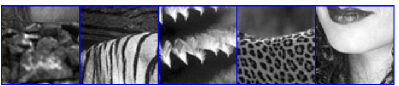
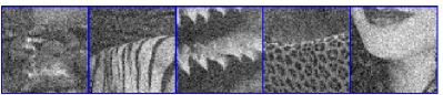
Figure 1: Subset of the ground truth and the noisy data with noise level $\sigma=25$.

IV-A Penalty functions

So far we have not designated the penalty function $\phi$ used in our training model. In this paper, we consider three penalty functions with different properties: (1) the $\ell_{1}$ norm, which is a well-known convex sparsity promoting function and has been successfully applied to a number of problems in image restoration [12], (2) the log-sum penalty suggested in [4], $\text{log}(1+|z|)$, which is a non-convex function and can enhance sparsity and (3) the smooth non-convex function $\text{log}(1+z^{2})$, which is derived from the student-t distribution and has been employed as the penalty function for sparse representation [37]. As our training model needs differentiable penalty functions, we have to use a small parameter $\varepsilon$ to regularize the absolute function $|z|$. The penalty functions and their associated derivatives are given by

$$\begin{cases}\phi(z)=\sqrt{z^{2}+\varepsilon^{2}}\\ \phi^{\prime}(z)=z/\sqrt{z^{2}+\varepsilon^{2}}\\ \phi^{\prime\prime}(z)=\varepsilon^{2}/(z^{2}+\varepsilon^{2})^{3/2}\end{cases} \begin{cases}\phi(z)=\text{log}(1+z^{2})\\ \phi^{\prime}(z)=2z/{(1+z^{2})}\\ \phi^{\prime\prime}(z)=2(1-z^{2})/{(1+z^{2})^{2}},\end{cases}$$ (IV.1)

and

$$\begin{cases}\phi(z)=\text{log}(1-\varepsilon+\sqrt{z^{2}+\varepsilon^{2}})\\ \phi^{\prime}(z)=\frac{z}{\sqrt{z^{2}+\varepsilon^{2}}(1-\varepsilon+\sqrt{z^{2}+\varepsilon^{2}})}\\ \phi^{\prime\prime}(z)=\frac{\varepsilon^{2}(1-\varepsilon)+(\varepsilon^{2}-z^{2})\sqrt{z^{2}+\varepsilon^{2}}}{(z^{2}+\varepsilon^{2})^{3/2}(1-\varepsilon+\sqrt{z^{2}+\varepsilon^{2}})^{2}}.\end{cases}$$

IV-B Training experiments

We focused training on filters of dimension $7\times 7$, since our approach allowed us to train larger filters than those trained in [34, 16], and normally larger filters can involve more information of the neighborhood. First, we conducted a preliminary training experiment based on the penalty function $\text{log}(1+z^{2})$. We intended to learn an analysis operator $A\in\mathbb{R}^{48\times 49}$, i.e, 48 filters with dimension $7\times 7$, and each filter is expressed as a linear combination of the DCT-7 basis. In principle, we can use any basis such as the identity, PCA or ICA basis; however as described below, we need zero-mean filters, which is guaranteed by the DCT filters after excluding the filter with constant entries.

For the preliminary experiment, we initialized the analysis operator using 48 random filters having unified norms and weights, which are 0.01 and 1, respectively. Finally training result shows that all the coefficients with respect to the first atom of DCT-7 (an atom with constant entries) are approximately equal to zero, implying that the first atom isn’t necessary to construct the filters. Therefore the learned filters are undoubtedly zero-mean because all the remaining atoms are zero-mean; this makes the analysis prior based model (III-A) illumination invariant. This result is coherent with the findings in the work [19] that meaningful filters should be zero-mean. Then we explicitly exclude the first atom in DCT-7 to speed up the training process for the following experiments.

We then conducted training experiments based on three different penalty functions. In this paper, the regularization parameter $\varepsilon$ in (IV.1) was set to $\varepsilon=10^{-2}$. Smaller $\varepsilon$ implies a better fitting to the absolute function, but it makes the lower-level problem harder to solve and the training algorithm fail. Just like in the preliminary experiment, we also learned 48 filters. We initialized the filters using the modified DCT-7 basis with unified norms and weights. The optimal analysis operator learned by using the penalty function $\text{log}(1+z^{2})$ is shown in Figure 2. The final loss function values (normalized by the number of training images) of these three experiments are presented in Table I (first three columns), together with the average denoising PSNR results based on 68 test images with $\sigma=25$ Gaussian noise.

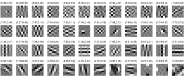
Figure 2: 48 filters of size $7\times 7$ learned by using the penalty function $\text{log}(1+z^{2})$. Each filter is shown with the corresponding norm and weight. The first number in the bracket is the weight $\alpha_{i}$ and the second one is the norm of the filter.

Final training results and the average denoising PSNR results on 68 test images
Penalty function	$|z|$	$\text{log}(1+|z|)$	$\text{log}(1+z^{2})$	$\text{log}(1+z^{2})$	$\text{log}(1+z^{2})$	$\text{log}(1+z^{2})$	$\text{log}(1+z^{2})$	$\text{log}(1+z^{2})$
Filter size	$7\times 7$	$7\times 7$	$7\times 7$	$7\times 7$	$9\times 9$	direct DCT-7	$5\times 5$	$3\times 3$
Number of filters	48	48	48	98	80	48	24	8
Final loss value	440,350	389,860	388,053	386,270	384,788	407,556	396,250	437,788
average PSNR	28.04	28.64	28.66	28.68	28.70	28.47	28.56	28.13

TABLE I: Summary of the final training loss values for different model capacities and the corresponding average denoising PSNR results based on 68 test images with $\sigma=25$ Gaussian noise.

As shown in Figure 2, the learned filters present some special structures. We can find high-frequency filters as well as derivative filters including the first derivatives along different directions, the second and the third derivatives. These filters make the analysis prior based model (III-A) a higher-order model which is able to capture the structures in natural images that cannot be captured by using only the first derivatives as in the total variation based methods.

In our training model, the size and the number of filters are free parameters; thus we can train filters of various sizes and numbers. Our current implementation is unoptimized Matlab code. The training time for 48 filters of size $7\times 7$ was approximately 24 hours on a server (Intel X5675, 3.07GHz), 98 filters of size $7\times 7$ took about 80 hours. However, the training time for larger filter size $9\times 9$ was much longer; it took about 20 days. Fortunately, the training procedure is off-line; thus the training time does not matter too much in practice. Demo training code can be downloaded from our homepage .

IV-C The influence of the penalty function

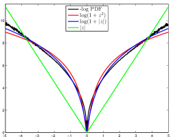
Figure 3: Negative log probability density function (PDF) of the filter response of a learned $7\times 7$ filter applied to natural images. Note that non-convex functions $\text{log}(1+|z|)$ and $\text{log}(1+z^{2})$ provide much better fits to the heavy tailed shape of the true density function, compared to the convex function $|z|$.

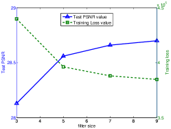
Figure 4: Performance curves (test PSNR value and training loss value) vs. the filter size. One can see that larger filter size can yield mprovements.

From Table I, we can see that the results obtained by two non-convex penalty functions, $\text{log}(1+|z|)$ and $\text{log}(1+z^{2})$ are very similar; however, there is a great improvement compared with the convex $\ell_{1}$ penalty function. The reason is as follows. It is well known that the probability density function (PDF) of the responses of zero-mean linear filters (e.g., DCT filters) applied to natural images exhibit heavy tailed distributions  [19]. Figure 3 shows the negative log PDF of the first filter in Figure 2 applied to natural images together with different model fits. We can clearly see that two non-convex functions, $\text{log}(1+|z|)$ and $\text{log}(1+z^{2})$ both provide an almost perfect fit to the heavy tailed shape of the true density function. The convex function $|z|$ presents a much worse fitting, however. Therefore, a suitable penalty function is crucial for the analysis-prior based model. In general, in order to model the heavy tailed shape of the true PDF, a non-convex function is required.

In order to further investigate how important the non-convex penalty function is for the analysis prior based model, we considered an analysis model consisting of 48 fixed and predefined filters (DCT-7 filters excluding the filter with uniform entries) and making use of the $\text{log}(1+z^{2})$ penalty function. We only optimized the norm and weight of each filter by using our bi-level training algorithm. The training loss value and the denoising test result of this model are shown in Table I (the sixth column entitled “direct DCT-7”). The image denoising test result is surprisingly good, even though this analysis model only utilizes a predefined analysis operator DCT-7. We will see in Table II of Section V that the performance of this model is already on par with the currently best analysis operator learning model - GOAL [17], which involves much more carefully trained filters. The success of this model lies in the non-convex penalty function $\text{log}(1+z^{2})$.

IV-D The influence of the number of filters

In previous work of analysis operator learning [31, 39, 17], the authors were interested in the over-complete case, where the number of filters is larger than the dimension of filters. Clearly our learned analysis operator in Figure 2 is under-complete. In order to investigate the influence of the over-complete property, we also conducted a training experiment for the over-complete case ($A\in\mathbb{R}^{98\times 49}$) based on the penalty function $\text{log}(1+z^{2})$. We initialized the analysis operator $A$ using 98 random zero-mean filters. The performance of this over-complete case is presented in Table I.

From Table I, one can see that the improvement achieved by over-complete analysis operator is marginal. Therefore for the analysis model, under-complete operators already work sufficiently well. An increase of the number of filters can not bring large improvements.

IV-E The influence of filter size

Intuitively the size of filters should be an important factor for the analysis model. In order to investigate the influence of filter size, we conducted training experiments for several different analysis models, where the filter size varies from $3\times 3$ to $9\times 9$. The training and evaluation results of these models are presented in Table I and Figure 4.

One can see that increasing the filter size yields some improvements. However, the performance is close to saturation when the filter size is increasing to $7\times 7$. The improvement brought by increasing the filter size to $9\times 9$ is negligible. This implies that we can not expect large improvements by increasing the filter size to $11\times 11$ or larger.

IV-F The robustness of our training scheme

As our training model (III.5) is a non-convex optimization problem, we can only find local minima. Thus a natural question about the initialization arises. We did have experiments for different initializations, such as random initialization. The final learned analysis operators are surely different, but all of them have almost the same training loss, which is the goal of our optimization problem. In addition, these operators perform similarly in evaluation experiments.

Another issue about the robustness of our training scheme is the influence of the training dataset. Since the training patches were randomly selected, we could run the training experiment multiple times by using a different training dataset. Finally, we found that the deviation of test PSNR values based on 68 test images is within 0.02dB, which is negligible.

V Application results using learned operators

An important question for a learned prior model is how well it generalizes. To evaluate this, we directly applied our learned analysis operators, which where trained for the image denoising task, to various image restoration problems such as image deconvolution, inpainting and super-resolution, as well as denoising. To start with, we first express the image restoration model by using our learned analysis operator, which is formulated as:

$$\arg\min\limits_{u}E(u)=\sum\nolimits_{i=1}^{n}\alpha_{i}\phi(\mathcal{A}_{i}u)+\frac{\lambda}{2}\|Ku-f\|_{2}^{2},$$ (V.1)

where $K$ is a linear operator which depends on the respective application to be handled.

To solve the minimization problem (V.1), for convex $\ell_{1}$ based model, we used the first-order primal-dual algorithm proposed in [5] with the preconditioning technique described in [29]; for non-convex penalty function based model, we employed L-BFGS for optimization. For L-BFGS, we need to calculate the gradient $\nabla_{u}E$, which includes constructing the highly sparse large matrix $\mathcal{A}_{i}$ and its transpose $\mathcal{A}_{i}^{T}$. This is quite time consuming in practice. In order to speed up the inference algorithm, we turn to a filtering technique as we know that $\mathcal{A}_{i}u$ is equivalent to the filtering operation ($A_{i}*u$). Therefore, the gradient $\nabla_{u}E$ is given by

$$\nabla_{u}E=\sum\nolimits_{i=1}^{n}\alpha_{i}A_{i}^{-}*\phi^{\prime}(A_{i}*u)+\lambda K^{T}(Ku-f),$$ (V.2)

where $A_{i}*u$ denotes the convolution of image $u$ with filter $A_{i}$, and $A_{i}^{-}$ denotes the filter obtained by mirroring $A_{i}$ around its center pixel (in practice, we need to carefully handle the boundaries as we need to ensure that the filters $A_{i}^{-}$ correspond to $\mathcal{A}_{i}^{T}$).

We provide Matlab demo code for training and denoising with penalty function $\text{log}(1+z^{2})$ on our homepage www.gpu4vision.org.

V-A Image denoising results

We first apply the analysis model based on our learned operators to the image denoising problem. In the case of image denoising, $K$ is simply the identity matrix, i.e., $K=\mathcal{I}$. Since the image denoising performance of one method varies greatly for different image contents, in order to make a fair comparison, we conducted denoising experiments over a standard test dataset - 68 Berkeley test images identified by Roth and Black [30]. We used exactly the same noisy version of each test image for different methods and different test images were added with distinct noise realizations. All results were computed per image and then averaged over the test dataset.

We considered image denoising for various noise levels $\sigma=\{15,25,50\}$. For noise levels other than $\sigma=25$, we need to tune the parameter $\lambda$ in (V.1). An empirical choice of $\lambda$ is: $\sigma=15$, $\lambda=25/\sigma\times 1.15$; $\sigma=50$, $\lambda=25/\sigma\times 0.8$.

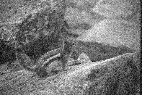
(a) noisy (20.17)

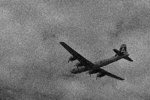
(b) noisy (20.17)

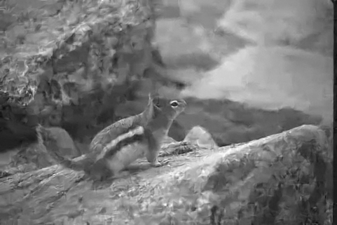
(c) $\text{log}(1+z^{2})$ (29.31)

(d) $\text{log}(1+z^{2})$ (36.84)

(e) $\text{log}(1+|z|)$ (29.34)

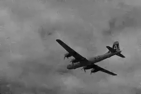
(f) $\text{log}(1+|z|)$ (36.40)

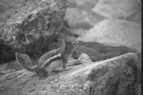
(g) $|z|$ (29.03)

(h) $|z|$ (34.24)

Figure 5: Comparison of denoising results obtained by three different penalty functions for noise level $\sigma=25$. The numbers shown in the brackets refer to PSNR values with respect to the clean images.

$\sigma$	KSVD	FoE	GOAL	BM3D	LSSC	EPLL	log$(1+z^{2})$ $7\times 7$, 48	log$(1+|z|)$ $7\times 7$, 48	$|z|$ $7\times 7$, 48	log$(1+z^{2})$ $7\times 7$, 98	log$(1+z^{2})$ $9\times 9$, 80	log$(1+z^{2})$ direct DCT-7
15	30.87	30.99	31.03	31.08	31.27	31.19	31.18	31.18	30.45	31.22	31.22	30.92
25	28.28	28.40	28.45	28.56	28.70	28.68	28.66	28.64	28.04	28.68	28.70	28.47
50	25.17	25.35	25.44	25.62	25.72	25.67	25.70	25.58	25.12	25.71	25.76	25.58

TABLE II: Summary of denoising results (average PSNR values). We highlighted the state-of-the-art results.

V-A1 Comparison of three different penalty functions

Table II shows the summary of denoising results achieved by different penalty functions. One can clearly see that two non-convex penalty functions lead to similarly good results and they significantly outperform the results of the convex function $|z|$. In addition, we can also see that the over-complete operator can not improve the performance too much and larger filters ($9\times 9$) can only achieve slightly better performance. Both of these two models are more time consuming than the model with 48 filters for inference; therefore, the analysis model based on 48 filters of size $7\times 7$ offers the best trade-off between computational cost and performance. In the following experiments, we only consider the model of 48 filters and the penalty function $\text{log}(1+z^{2})$. We prefer the penalty function $\text{log}(1+z^{2})$, since it is completely smooth, making the corresponding minimization problem easier to solve. We present two denoising examples obtained by three different penalty functions in Figure 5.

V-A2 Comparison to other analysis models

Our learned model is an analysis prior-based model, but can also be viewed as a MRF-based system. In order to rank our model among other analysis models, we compared its performance with existing analysis models, including typical FoE models [30, 34, 33, 3, 11, 16] and the currently published best analysis operator model - GOAL [17]. For the GOAL method, we made use of the $l_{0.4}$-norm penalty function $|z|^{0.4}$, together with the learned analysis operator $\Omega\in\mathbb{R}^{98\times 49}$ provided by the authors. We also utilized the L-BFGS algorithm to solve the corresponding minimization problem. We present image denoising results of all approaches over 68 test images with noise level $\sigma=25$ in Table III. One can see that our model based on the penalty function $\text{log}(1+z^{2})$ (48 learned filters, $7\times 7$) has achieved the best performance among all the related approaches. The comparison with the best FoE [16] model and the latest analysis model GOAL for other noise levels is shown in Table II. For all the noise levels, our trained analysis model outperforms both of them significantly.

An interesting result in Table II is that the performance of the direct DCT-7 model, which only utilizes a predefined analysis operator DCT-7 (48 filters of size $7\times 7$), is already on par with the GOAL model, which involves much more carefully trained filters (98 filters of size $7\times 7$). For this direct DCT-7 model, we used the $\text{log}(1+z^{2})$ penalty function, and only optimized the norms and weights of the filters using our bi-level training algorithm. This result demonstrates the importance of non-convex penalty functions and the effectiveness of our bi-level training scheme.

As the analysis operator of GOAL model is trained using a patch-based model, we can also use it in the manner of patch-averaging to conduct image denoising like K-SVD [13]. We embedded the learned analysis operator $\Omega$ into the patch-based analysis model (I.2), and used it to denoise each patch extracted from an image. We also considered overlapped windows and averaged the results in the overlapping regions to form the final denoised image. As expected, we got inferior results (average PSNR 28.25 over 68 test images) to the model formulated under the FoE framework (average PSNR 28.45).

model	potential	training	PSNR
$5\times 5$ FoE	ST&GLP.	contrastive divergence	27.77[30]
$3\times 3$ FoE	GSMs	contrastive divergence	27.95[34]
$5\times 5$ FoE	GSMs	persistent contrastive divergence	28.40[16]
$5\times 5$ FoE	ST	bi-level (truncated optimization)	28.24[3]
$5\times 5$ FoE	ST	bi-level (truncated optimization)	28.39[11]
$5\times 5$ FoE	ST	bi-level (implicit differentiation)	27.86[33]
$7\times 7$
GOAL	GLP	geometric conjugate gradient	28.45[17]
$7\times 7$ FoE	ST	bi-level (implicit differentiation)	28.66

TABLE III: Summary of various analysis models and the average denoising results on 68 test images with $\sigma=25$. We highlighted our result, also the best one.

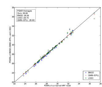
Figure 6: Scatter plot of the PSNRs over 68 Berkeley images produced by our learned log($1+z^{2}$)-based analysis model, BM3D, GMM-EPLL and LSSC. A point above the line $y=x$ means a better performance than our model.

V-A3 Comparison to state-of-the-art methods

In order to evaluate how well our analysis models work for the denoising task, we compared their performance with leading image denoising methods, including three state-of-the-art methods: (1) BM3D [9]; (2) LSSC [25]; (3) GMM-EPLL [41] along with three leading generic methods: (4) a MRF-based approach, FoE [16]; (5) a synthesis sparse representation based method, KSVD [13] trained on natural image patches; and (6) the currently published best analysis operator learning method, GOAL [17]. All implementations were downloaded from the corresponding authors’ homepages. We conducted denoising experiments over 68 Berkeley test images with various noise levels $\sigma=\{15,25,50\}$. All results were computed per image and then averaged over the number of images.

Table II shows the summary of results. One can see that our trained model based on the penalty function $\text{log}(1+z^{2})$ (48 learned filters, $7\times 7$) outperforms three leading generic methods and is on par with three state-of-the-art methods for any noise level. To the best of our knowledge, this is the first time that a MRF model based on generic priors of natural images has achieved such clear state-of-the-art performance. Figure 6 gives a detailed comparison between our learned analysis model and three state-of-the-art methods over 68 test images for $\sigma=25$. We can see that all the points surround the diagonal line “$y=x$” closely, i.e., all considered methods achieve very similar results. Therefore, it is clear that our learned analysis models based on non-convex penalty functions are state-of-the-art. We present an image denoising example of the considered methods in Figure 7.

(a) clean image

(b) $\sigma=25$ (20.17)

(c) KSVD (29.13)

(d) FoE (29.15)

(e) BM3D (29.52)

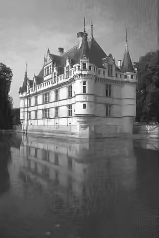
(f) LSSC (29.47)

(g) GMM-EPLL (29.50)

(h) GOAL (29.30)

(i) $\text{log}(1+z^{2})$ (29.48)

Figure 7: The images $(c)\sim(i)$ present results achieved by the compared methods for denoising “water-castle” image corrupted with $\sigma=25$.

Our model is well-suited to GPU parallel computation since it solely contains convolution of filters with an image. Our GPU implementation based on a NVIDIA Geforce GTX 580 accelerates the inference procedure significantly; for a denoising task with $\sigma=25$, typically it takes 0.87s for image size $512\times 512$, 0.60s for $481\times 321$ and 0.29s for $256\times 256$, i.e., using our GPU based implementation, image denoising can be conducted in near real-time at 3.4fps for an $256\times 256$ image sequence, with state-of-the-art performance. In Table IV, we show the average running time of the considered denoising methods on $481\times 321$ images.

Considering the speed and quality of our model, it is a perfect choice as a base method in the image restoration framework proposed in [20], which leverages advantages of existing methods.

V-B Single image super-resolution

For single image super-resolution, the linear operator $K$ is constructed by a decimation operator $\Phi$ and a blurring operator $B$, i.e., $K=\Phi B$. In order to perform a better comparison with the latest analysis model GOAL [17], we conducted the same single image super-resolution experiment. We artificially created a low resolution image by downsampling a ground-truth image by a factor of 3 using bicubic interpolation. Then the low resolution image was corrupted by Gaussian noise with $\sigma=8$. We magnified the noisy low resolution image by the same factor using (a) bicubic interpolation, (b) GOAL method [17], (c) our learned analysis model based on penalty function log$(1+z^{2})$ respectively. Figure 8 shows the results for different methods. One can see that two analysis models present similar results, which are visually and quantitatively better than the bicubic method.

(a) Original image

(b) Bicubic interpolation (21.63)

(c) GOAL [17] (23.45)

(d) Ours: log$(1+z^{2})$ (23.50)

Figure 8: Single image super-resolution results for magnifying a noisy low resolution image by a factor of 3. The low resolution image was degraded by Gaussian noise with $\sigma=8$. The numbers shown in the brackets refer to PSNR values with respect to the clean image.

	KSVD	FoE	BM3D	LSSC	EPLL	GOAL	ours
T(s)	30	1600	4.3	700	99	112	12 (0.6)
psnr	28.28	28.40	28.56	28.70	28.68	28.45	28.66

TABLE IV: Typical run time of the denoising methods for a $481\times 321$ image ($\sigma=25$) on a server (Intel X5675, 3.07GHz). The highlighted number is the run time of the GPU implementation.

V-C Non-blind image deconvolution

In the case of image deconvolution, $Ku$ can be written as a convolution, i.e., $Ku=k_{K}*u$, where $k_{K}$ is the convolution kernel. We considered a non-blind image deconvolution task, where a clean image was degraded by a motion blur of approximately 20 pixels and slight Gaussian noise with noise level $\sigma=2.5$. Again, we used our learned analysis models based on the log$(1+z^{2})$ penalty function for image deblurring. In order to present a comparison, we also conducted deblurring by using the GMM-EPLL model [41] and the latest analysis operator learning algorithm GOAL [17]. For the GOAL method, we utilized the learned analysis operator $\Omega\in\mathbb{R}^{98\times 49}$ provided by the authors. Figure 9 shows the motion deblurring results achieved by our model, GMM-EPLL and GOAL, respectively. We can see that our learned analysis model yields better results in terms of PSNR.

(a) Original image

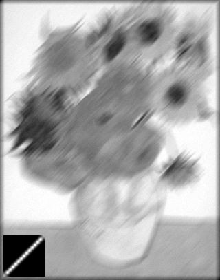
(b) Degraded image

(c) GMM-EPLL (27.46)

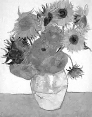
(d) GOAL (27.97)

(e) log$(1+z^{2})$ (28.26)

Figure 9: Motion deblurring results of our learned analysis model, the GMM-EPLL model [41] and the GOAL model [17]. The degraded image is generated using a motion blur of approximately 20 pixels and a Gaussian noise of $\sigma=2.5$.

V-D Image inpainting

Image inpainting is the process of filling in lost image data such that the resulting image is visually appealing. Typically, the positions of the pixels to be filled up are given. In our formulation, the linear operator $K$ is simply a sampling matrix, where each row contains exactly one entry equal to one. Its position indicates a pixel with given value. The parameter $\lambda$ corresponds to joint inpainting and denoising, and the choice $\lambda\rightarrow+\infty$ means pure inpainting. In our experiment since we assumed the test images are noise free, we empirically selected $\lambda=10^{3}$. Due to space limitation, we only considered a classical image inpainting task here.

We destroyed the ground-truth “ Lena” image ($512\times 512$) artificially by masking 90% of the entire pixels randomly as shown in Figure 10(a). Then we reconstructed the incomplete image using our learned analysis model - log($1+z^{2}$)-based model. In order to present a comparison, we also give the inpainting result of the GOAL model [17] and FoE model [30]. From Figure 10, one can see that the result of our learned analysis model based on log($1+z^{2}$) penalty achieves equivalent results with respect to the GOAL model.

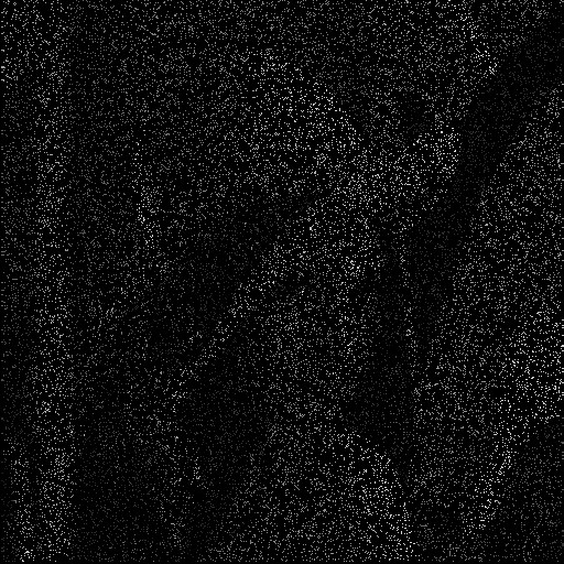
(a) 90 % missing pixels

(b) FoE (28.06)

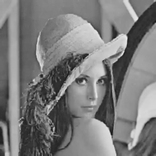
(c) GOAL (28.57)

(d) log$(1+z^{2})$ (28.62)

Figure 10: Recovery results of the destroyed “Lena”  image with 90% loss pixels using our learned analysis model, a recent analysis model - GOAL [17] and the FoE model [30].

VI Conclusion and outlook

In this paper, we have expressed our insights into the co-sparse analysis model. We propose to go beyond existing patch-based models, and to exploit the framework of FoE model to define a image prior over the entire image, rather than image patches. We have pointed out that the image based analysis model is equivalent to the FoE model. Starting from this conclusion, we have introduced a bi-level training approach for analysis operator learning, which is solved effectively with L-BFGS algorithm. By using our training framework, we have carefully investigated the effect of different aspects of the analysis prior model including the filter size, the number of filters and the penalty function.

Since our training scheme directly optimizes the MAP-inference based analysis model, the learned model is an optimal MAP inference for image restoration problems. Numerical results have confirmed the good performance of our learned analysis model. For classic tasks such as image denoising, image deconvolution, image super-resolution and image inpainting, our learned analysis model has achieved strongly competitive performance with current state-of-the-art methods, and clearly outperforms existing analysis learning approaches.

For future work, focusing on generic priors of natural images, we expect that our learned analysis model could be improved potentially in two aspects: (1) consider more flexible penalty function. In our current model, the penalty function is fixed to the same form for every filter. If we free the shape of the penalty function, our model will possess more freedom, which might increase the performance. A feasible way to consider alterable penalty function is to make use of the GSMs prior [34]. (2) make use of larger training dataset. Our training is conducted based on 200 training samples, which is only a very small part of the natural images. Consequently, the learned filters may over-fit on the training dataset. However, our current training scheme is not available for large training dataset, e.g., $\sim 10^{6}$, because it needs to solve the lower-level problem for each training sample. Feasible methods may include making use of stochastic optimization.

VII Acknowledgments

The authors wish to thank Qi Gao (TU Darmstadt) for sharing details of the FoE model; Daniel Zoran (Hebrew University of Jerusalem) for sharing testing details for the GMM-EPLL algorithm; Simon Hawe (TU Munich) for useful discussion about analysis operator learning.

Yunjin Chen received the B.Sc. degree in applied physics from Nanjing University of Aeronautics and Astronautics, Jiangsu, China, and the M.Sc. degree in optical engineering from National University of Defense Technology, Hunan, China, in 2007 and 2009, respectively. Since September 2011, he has been pursing the Ph.D degree at the Institute for Computer Graphics and Vision, Graz University of Technology. His current research interests are learning image prior model for low-level computer vision problems and convex optimization.

René Ranftl received the B.Sc. degree and M.Sc. degree in Telematics from Graz University of Technology in 2009 and 2010, respectively. Since 2010 he has been pursuing the Ph.D. degree at the Institute for Computer Graphics and Vision, Graz University of Technology. His current research interests include image sequence analysis, 3D reconstruction and machine learning.

Thomas Pock received a M.Sc and a Ph.D degree in Telematik from Graz University of Technology in 2004 and 2008, respectively. He is currently employed as an Assistant Professor at the Institute for Computer Graphics and Vision at Graz University of Technology. In 2013 he received the START price of the Austrian Science Fund (FWF) and the German Pattern recognition award of the German association for pattern recognition (DAGM). His research interests include convex optimization and in particular variational methods with application to segmentation, optical flow, stereo, registration as well as its efficient implementation on parallel hardware.

References

- [1] M. Aharon, M. Elad, and A. Bruckstein. K-SVD: An algorithm for designing over-complete dictionaries for sparse representation. IEEE Transactions on Signal Processing, 54(11):4311–4322, 2006.
- [2] P. Arbelaez, M. Maire, C. Fowlkes, and J. Malik. Contour detection and hierarchical image segmentation. IEEE Trans. Pattern Anal. Mach. Intell., 33(5):898–916, May 2011.
- [3] A. Barbu. Training an active random field for real-time image denoising. IEEE Trans. on Image Proc, 18(11):2451–2462, 2009.
- [4] E. J. Candès, M. B. Wakin, and S. P. Boyd. Enhancing sparsity by reweighted l1 minimization. J. Fourier Analysis and Applications, 14:877–905, 2008.
- [5] A. Chambolle and T. Pock. A first-order primal-dual algorithm for convex problems with applications to imaging. Journal of Mathematical Imaging and Vision, 40(1):120–145, 2011.
- [6] Y. J. Chen, T. Pock, and H. Bischof. Learning -based analysis and synthesis sparsity priors using bi-level optimization. In Workshop on Analysis Operator Learning vs. Dictionary Learning, NIPS 2012, 2012.
- [7] Y. J. Chen, T. Pock, R. Ranftl, and H. Bischof. Revisiting loss-specific training of filter-based MRFs for image restoration. In GCPR, 2013.
- [8] B. Colson, P. Marcotte, and G. Savard. An overview of bilevel optimization. Annals OR, 153(1):235–256, 2007.
- [9] K. Dabov, A. Foi, V. Katkovnik, and K. O. Egiazarian. Image denoising by sparse 3-d transform-domain collaborative filtering. IEEE Transactions on Image Processing, 16(8):2080–2095, 2007.
- [10] C. B. Do, C.-S. Foo, and A. Y. Ng. Efficient multiple hyperparameter learning for log-linear models. In NIPS, 2007.
- [11] J. Domke. Generic methods for optimization-based modeling. Journal of Machine Learning Research - Proceedings Track, 22:318–326, 2012.
- [12] D. L. Donoho, M. Elad, and V. N. Temlyakov. Stable recovery of sparse overcomplete representations in the presence of noise. IEEE Transactions on Information Theory, 52(1):6–18, 2006.
- [13] M. Elad and M. Aharon. Image denoising via sparse and redundant representations over learned dictionaries. IEEE Transactions on Image Processing, 15(12):3736–3745, 2006.
- [14] M. Elad, P. Milanfar, and R. Rubinstein. Analysis versus synthesis in signal priors. Inverse Problems, 23(3):947–968, 2007.
- [15] M.-J. Fadili, J.-L. Starck, and F. Murtagh. Inpainting and zooming using sparse representations. Comput. J., 52(1):64–79, 2009.
- [16] Q. Gao and S. Roth. How well do filter-based MRFs model natural images? In DAGM/OAGM Symposium, pages 62–72, 2012.
- [17] S. Hawe, M. Kleinsteuber, and K. Diepold. Analysis operator learning and its application to image reconstruction. IEEE Transactions on Image Processing, 22(6):2138–2150, 2013.
- [18] G. E. Hinton. Products of experts. In ICANN, pages 1–6, 1999.
- [19] J. Huang and D. Mumford. Statistics of natural images and models. In IEEE Conference on Computer Vision and Pattern Recognition (CVPR1999), pages 541–547, Fort Collins, CO, USA, 1999.
- [20] J. Jancsary, S. Nowozin, and C. Rother. Loss-specific training of non-parametric image restoration models: A new state of the art. In ECCV, pages 112–125, 2012.
- [21] K. Kunisch and T. Pock. A bilevel optimization approach for parameter learning in variational models. SIAM Journal on Imaging Sciences, 6(2):938–983, 2013.
- [22] H. Lee, A. Battle, R. Raina, and A. Y. Ng. Efficient sparse coding algorithms. In NIPS, pages 801–808, 2006.
- [23] D. C. Liu and J. Nocedal. On the limited memory BFGS method for large scale optimization. Mathematical Programming, 45(1):503–528, 1989.
- [24] J. Mairal, F. Bach, J. Ponce, and G. Sapiro. Online dictionary learning for sparse coding. In ICML, pages 689–696, 2009.
- [25] J. Mairal, F. Bach, J. Ponce, G. Sapiro, and A. Zisserman. Non-local sparse models for image restoration. In ICCV, pages 2272–2279, 2009.
- [26] J. Mairal, M. Elad, and G. Sapiro. Sparse representation for color image restoration. IEEE Transactions on Image Processing, 17(1):53–69, 2008.
- [27] B. Ophir, M. Elad, N. Bertin, and M. D. Plumbley. Sequential minimal eigenvalues – an approach to analysis dictionary learning. In European Signal Processing Conference, pages 1465–1469, 2011.
- [28] G. Peyré and J. Fadili. Learning analysis sparsity priors. In Proc. of Sampta’11, 2011.
- [29] T. Pock and A. Chambolle. Diagonal preconditioning for first order primal-dual algorithms. In ICCV, 2011.
- [30] S. Roth and M. J. Black. Fields of experts. International Journal of Computer Vision, 82(2):205–229, 2009.
- [31] R. Rubinstein, T. Faktor, and M. Elad. K-SVD dictionary-learning for the analysis sparse model. In ICASSP, 2012.
- [32] R. Rubinstein, T. Peleg, and M. Elad. Analysis K-SVD: A dictionary-learning algorithm for the analysis sparse model. IEEE Transactions on Signal Processing, 61(3):661–677, 2013.
- [33] K. G. G. Samuel and M. Tappen. Learning optimized map estimates in continuously-valued MRF models. In CVPR, 2009.
- [34] U. Schmidt, Q. Gao, and S. Roth. A generative perspective on MRFs in low-level vision. In CVPR, pages 1751–1758, 2010.
- [35] M. F. Tappen. Utilizing variational optimization to learn markov random fields. In CVPR, pages 1–8, 2007.
- [36] M. F. Tappen, K. G. G. Samuel, C. V. Dean, and D. M. Lyle. The logistic random field - a convenient graphical model for learning parameters for MRF-based labeling. In CVPR, 2008.
- [37] Y. W. Teh, M. Welling, S. Osindero, and G. E. Hinton. Energy-based models for sparse overcomplete representations. Journal of Machine Learning Research, 4:1235–1260, 2003.
- [38] M. Welling, G. E. Hinton, and S. Osindero. Learning sparse topographic representations with products of student-t distributions. In NIPS, pages 1359–1366, 2002.
- [39] M. Yaghoobi, S. Nam, R. Gribonval, and M. E. Davies. Analysis operator learning for over-complete co-sparse representations. In European Signal Processing Conference, 2011.
- [40] M. Yaghoobi, S. Nam, R. Gribonval, and M. E. Davies. Noise aware analysis operator learning for approximately cosparse signals. In ICASSP, 2012.
- [41] D. Zoran and Y. Weiss. From learning models of natural image patches to whole image restoration. In ICCV, pages 479–486, 2011.