Asymptotic behavior and distributional limits of preferential attachment graphs

Abstract

We give an explicit construction of the weak local limit of a class of preferential attachment graphs. This limit contains all local information and allows several computations that are otherwise hard, for example, joint degree distributions and, more generally, the limiting distribution of subgraphs in balls of any given radius $k$ around a random vertex in the preferential attachment graph. We also establish the finite-volume corrections which give the approach to the limit.

, ,
and

1 Introduction

About a decade ago, it was realized that the Internet has a power-law degree distribution Faloutsos , AJB99 . This observation led to the so-called preferential attachment model of Barabási and Albert Barabasi1 , which was later used to explain the observed power-law degree sequence of a host of real-world networks, including social and biological networks, in addition to technological ones. The first rigorous analysis of a preferential attachment model, in particular proving that it has small diameter, was given by Bollobás and Riordan brdiam . Since these works there has been a tremendous amount of study, both nonrigorous and rigorous, of the random graph models that explain the power-law degree distribution; see BAreview and BRreview and references therein for some of the nonrigorous and rigorous work, respectively.

Also motivated by the growing graphs appearing in real-world networks, for the past five years or so, there has been much study in the mathematics community of notions of graph limits. In this context, most of the work has focused on dense graphs. In particular, there has been a series of papers on a notion of graph limits defined via graph homomorphisms BCLSV-rev , dense1 , dense2 , LSz ; these have been shown to be equivalent to limits defined in many other senses dense1 , dense2 . Although most of the results in this work concern dense graphs, the paper BCLSV-rev also introduces a notion of graph limits for sparse graphs with bounded degrees in terms of graph homomorphisms; using expansion methods from mathematical physics, Borgs et al. sparse establishes some general results on this type of limit for sparse graphs. Another recent work BR07 concerns limits for graphs which are neither dense nor sparse in the above senses; they have average degrees which tend to infinity.

Earlier, a notion of a weak local limit of a sequence of graphs with bounded degrees was given by Benjamini and Schramm BS01 (this notion was in fact already implicit in Ald99 ). Interestingly, it is not hard to show that the Benjamini–Schramm limit coincides with the limit defined via graph homomorphisms in the case of sparse graphs of bounded degree; see Elek for yet another equivalent notion of convergent sequences of graphs with bounded degrees.

As observed by Lyons Lyo05 , the notion of graph convergence introduced by Benjamini and Schramm is meaningful even when the degrees are unbounded, provided the average degree stays bounded. Since the average degree of the Barabási–Albert graph is bounded by construction, it is therefore natural to ask whether this graph sequence converges in the sense of Benjamini and Schramm.

In this paper, we establish the existence of the Benjamini–Schramm limit for the Barabási–Albert graph by giving an explicit construction of the limit process, and use it to derive various properties of the limit. Our results cover the case of both uniform and preferential attachments graphs. Moreover, our methods establish the finite-volume corrections which give the approach to the limit.

Our proof uses a representation, which we first introduced in BBCS05 , to analyze processes that model the spread of viral infections on preferential attachment graphs. Our representation expresses the preferential attachment model process as a combination of several Pólya urn processes. The classic Pólya urn model was of course proposed and analyzed in the beautiful work of Pólya and Eggenberger in the early twentieth century EP ; see durrett for a basic reference. Despite the fact that our Pólya urn representation is a priori only valid for a limited class of preferential attachment graphs, we give an approximating coupling which proves that the limit constructed here is the limit of a much wider class of preferential attachment graphs.

Our alternative representation contains much more independence than previous representations of preferential attachment and is therefore simpler to analyze. In order to demonstrate this, we also give a few applications of the limit. In particular, we use the limit to calculate the degree distribution and the joint degree distribution of a typical vertex with the vertex it attached to in the preferential attachment process (more precisely, a vertex chosen uniformly from the ones it attached to).

2 Definition of the model and statements of results

2.1 Definition of the model

The preferential attachment graph we define generalizes the model introduced by Barabási and Albert Barabasi1 and rigorously constructed in brdiam . Fix an integer $m\geq 2$ and a real number $0\leq\alpha<1$. We will construct a sequence of graphs $(G_{n})$ (where $G_{n}$ has $n$ vertices labeled $1,\ldots,n$) as follows:

$G_{1}$ contains one vertex and no edges, and $G_{2}$ contains two vertices and $m$ edges connecting them. Given $G_{n-1}$ we create $G_{n}$ the following way: we add the vertex $n$ to the graph, and choose $m$ vertices $w_{1},\ldots,w_{m}$, possibly with repetitions, from $G_{n-1}$. Then we draw edges between $n$ and each of $w_{1},\ldots,w_{m}$. Repetitions in the sequence $w_{1},\ldots,w_{m}$ result in multiple edges in the graph $G_{n}$.

We suggest three different ways of choosing the vertices $w_{1},\ldots,w_{m}$. The first two ways, the independent and the conditional, are natural ways which we consider of interest, and are the two most common interpretations of the preferential attachment model. The third way, that is, the sequential model, is less natural, but is much easier to analyze because it is exchangeable, and therefore by de-Finetti’s theorem (see durrett ) has an alternative representation, which contains much more independence. We call this representation the Pólya urn representation because the exchangeable system we use is the Pólya urn scheme.

1. [(2)]

2. The independent model: $w_{1},\ldots,w_{m}$ are chosen independently of each other conditioned on the past, where for each $i=1,\ldots,m$, we choose $w_{i}$ as follows: with probability $\alpha$, we choose $w_{i}$ uniformly from the vertices of $G_{n-1}$, and with probability $1-\alpha$, we choose $w_{i}$ according to the preferential attachment rule, that is, for all $k=1,\ldots,n-1$,

   $${\mathbf{P}}(w_{i}=k)=\frac{\deg_{n-1}(k)}{Z},$$

   where $Z$ is the normalizing constant $Z=\sum_{k=1}^{n-1}\deg_{n-1}(k)=2m(n-2)$.

3. The conditional model: here we start with some predetermined graph structure for the first $m$ vertices. Then at each step, $w_{1},\ldots,w_{m}$ are chosen as in the independent case, conditioned on them being different from one another.

4. The sequential model: $w_{1},\ldots,w_{m}$ are chosen inductively as follows: with probability $\alpha$, $w_{1}$ is chosen uniformly, and with probability $1-\alpha$, $w_{1}$ is chosen according to the preferential attachment rule, that is, for every $k=1,\ldots,n-1$, we take $w_{1}=k$ with probability $(\deg_{n-1}(k))/Z$ where as before $Z=2m(n-2)$. Then we proceed inductively, applying the same rule, but with two modifications:

   1. [(a)]

   2. When determining $w_{i}$, instead of the degree $\deg_{n-1}(k)$, we use

      $$\deg^{\prime}_{n-1}(k)=\deg_{n-1}(k)+\#\{1\leq j\leq i-1\mid w_{j}=k\}$$

      and normalization constant

      $$Z^{\prime}=\sum_{k=1}^{n-1}\bigl{(}\deg^{\prime}_{n-1}(k)\bigr{)}=2m(n-2)+i-1.$$

   3. The probability of uniform connection will be

      $$\tilde{\alpha}=\alpha\frac{2m(n-1)}{2m(n-2)+2m\alpha+(1-\alpha)(i-1)}=\alpha+O\bigl{(}n^{-1}\bigr{)}$$ (1)

      rather than $\alpha$.

We will refer to all three models as versions of the preferential attachment graph, or PA-graph, for short. Even though we consider the graph $G_{n}$ as undirected, it will often be useful to think of the vertices $w_{1},\ldots,w_{m}$ as vertices which “received an edge” from the vertex $n$, and of $n$ as a vertex which “sent out $m$ edges” to the vertices $w_{1},\ldots,w_{m}$. Note in particular, that the degree of a general vertex $v$ in $G_{n}$ can be written as $m+q$, where $m$ is the number of edges sent out by $v$ and $q$ is the (random) number of edges received by $v$.

2.2 Pólya urn representation of the sequential model

Our first theorem gives the Pólya urn representation of the sequential model. To state it, we use the standard notation $X\sim\beta(a,b)$ for a random variable $X\in[0,1]$ whose density is equal to $\frac{1}{Z}x^{a-1}(1-x)^{b-1}$, where $Z=\int_{0}^{1}x^{a-1}(1-x)^{b-1}\,dx$. We set

$$u=\frac{\alpha}{1-\alpha}.$$

Note that $u\in[0,\infty)$.

Theorem 2.1

Fix $m$, $\alpha$ and $n$. Let $\psi_{1}=1$, let $\psi_{2},\ldots,\psi_{n}$ be independent random variables with

$$\psi_{j}\sim\beta\bigl{(}m+2mu,(2j-3)m+2mu(j-1)\bigr{)}$$ (2)

and let

$$\varphi_{j}=\psi_{j}\prod_{i=j+1}^{n}(1-\psi_{i}),\qquad S_{k}=\sum_{j=1}^{k}\varphi_{j}\quad\mbox{and}\quad I_{k}=[S_{k-1},S_{k}).$$ (3)

Conditioned on $\psi_{1},\ldots,\psi_{n}$, choose $\{U_{k,i}\}_{k=1,\ldots,n,i=1,\ldots,m}$ as a sequence of independent random variables, with $U_{{k,i}}$ chosen uniformly at random from $[0,S_{k-1}]$. Join two vertices $j$ and $k$ if $j<k$ and $U_{k,i}\in I_{j}$ for some $i\in\{1,\ldots,m\}$ (with multiple edges between $j$ and $k$ if there are several such $i$). Denote the resulting random multi-graph by $G_{n}$.

Then $G_{n}$ has the same distribution as the sequential PA-graph.

Figure 1 illustrates this theorem.

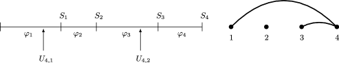
Figure 1: The Pólya-representation of the sequential model for $m=2$, $n=4$ and $k=4$. The variables $U_{4,1}$ and $U_{4,2}$ are chosen uniformly at random from $[0,S_{3}]$.

It should be noted that the $\alpha=0$ case of the sequential model defined here differs slightly from the model of Bollobás and Riordan brdiam in that they allow (self-)loops, while we do not. In fact, a minor alteration of our Pólya urn representation models their graph, and we suspect that a minor alteration of their pairing representation can model our graph.

2.3 Definition of the Pólya-point graph model

2.3.1 Motivation

The Benjamini–Schramm notion BS01 of weak convergence involves the view of the graph $G_{n}$ from the point of view of a “root” $k_{0}$ chosen uniformly at random from all vertices in $G_{n}$. More precisely, it involves the limit of the sequence of balls of radius $1,2,\ldots\,$, about this root; see Definition 2.1 in Section 2.4 below for the details.

It turns out that for the sequential model, this limit is naturally described in terms of the random variables $S_{k-1}$ introduced in Theorem 2.1. To explain this, it is instructive to first consider the ball of radius $1$ around the random root $k_{0}$. This ball contains the $m$ neighbors of $k_{0}$ that were born before $k_{0}$ and received an edge from $k_{0}$ under the preferential attachment rule described above, as well as a random number $q_{0}$ of neighbors that were born after $k_{0}$ and send an edge to $k_{0}$ at the time they were born. We denote these neighbors by $k_{01},\ldots,k_{0m}$ and $k_{0,m+1},\ldots,k_{0,m+q_{0}}$, respectively.

Let

$$\chi=\frac{1+2u}{2+2u}\quad\mbox{and}\quad\psi=\frac{1-\chi}{\chi}{=\frac{1}{1+2u}}$$ (4)

and note that $\frac{1}{2}\leq\chi<1$ and $0<\psi\leq 1$. As we will see, the random variables $S_{k-1}$ behave asymptotically like $(k/n)^{\chi}$, implying in particular that the distribution of $S_{k_{0}-1}$ tends to that of a random variable $x_{0}=y_{0}^{\chi}$, where $y_{0}$ is chosen uniformly at random in $[0,1]$. The limiting distribution of $S_{k_{01}-1},\ldots,S_{k_{0m}-1}$ turns out to be quite simple as well: in the limit these random variables are i.i.d. random variables $x_{0,i}$ chosen uniformly from $[0,x_{0}]$, a distribution which is more or less directly inherited from the uniform random variables $U_{k,i}\in[0,S_{k_{0}-1}]$ from Theorem 2.1. The limiting distribution of the random variables $S_{k_{0,m+1}-1},\ldots,S_{k_{0,m+q_{0}}-1}$ is slightly more complicated to derive and is given by a Poisson process in $[x_{0},1]$ with intensity

$${\gamma_{0}\frac{\psi x^{\psi-1}}{x_{0}^{\psi}}\,dx.}$$

Here $\gamma_{0}$ is a random “strength” which arises as a limit of the $\beta$-distributed random variable $\psi_{k_{0}}$, and is distributed according to $\Gamma({m+2mu},1)$. Here, as usual, $\Gamma(a,b)$ is used to denote a distribution on $[0,\infty)$ which has density $\frac{1}{Z}x^{a-1}e^{-bx}$, with $Z=\int_{0}^{\infty}x^{a-1}e^{-bx}\,dx$.

Next, consider the branching that results from exploring the neighborhood of a random vertex in $G_{n}$ in a ball of radius bigger than one. In each step of this exploration, we will find two kinds of children of the current vertex $k$: those which were born before $k$, and were attached to $k$ at the birth of $k$, and those which were born after $k$, and were connected to $k$ at their own birth. There are always either $m$ or $m-1$ children of the first kind (if $k$ was born after its parent, there will be $m-1$ such children, since one of the $m$ edges sent out by $k$ was sent out to $k$’s parent; otherwise there will be $m$ children of the first type). The number of children of the second kind is a random variable.

In the limit $n\to\infty$, this branching process leads to a random tree whose vertices, $\bar{a}$, carry three labels: a “strength” $\gamma_{\bar{a}}\in(0,\infty)$ inherited from the $\beta$-random variables $\psi_{k}$, a “position” $x_{\bar{a}}\in[0,1]$ inherited from the random variables $S_{k-1}$ and a type which can be either $L$ (for “left”) or $R$ (for “right”), reflecting whether the vertex $k$ was born before or after its parent. While the strengths of vertices of type $R$ turn out to be again $\Gamma({m+2mu},1)$-distributed, this is not the case for vertices of type $L$, since a vertex with higher values of $\psi_{k}$ has a larger probability of receiving an edge from its child. In the limit, this will be reflected by the fact that the strength of vertices of type $L$ is $\Gamma({m+2mu}+1,1)$-distributed.

2.3.2 Formal definition

The main goal of the previous subsection was to give an intuition of the structure of the neighborhood of a random vertex. We will show that asymptotically, the branching process obtained by exploring the neighborhood of a random vertex $k_{0}$ in $G_{n}$ is given by a random tree with a certain distribution. In order to state our main theorem, we give a formal definition of this tree.

Let $F$ be the Gamma distribution $\Gamma({m+2mu},1)$, and let $F^{\prime}$ be the Gamma distribution $\Gamma({m+2mu+1},1)$. We define a random, rooted tree $(T,0)$ with vertices labeled by finite sequences

$$\bar{a}=(0,a_{1},a_{2},\ldots,a_{l})$$

inductively as follows:

• The root $(0)$ has a position $x_{0}=y_{0}^{\chi}$, where $y_{0}$ is chosen uniformly at random in $[0,1]$. In the rest of the paper, for notational convenience, we will write $0$ instead of $(0)$ for the root.

• In the induction step, we assume that $\bar{a}=(0,a_{1},a_{2},\ldots,a_{l})$ and the corresponding variable $x_{\bar{a}}\in[0,1]$ have been chosen in a previous step. Define $(\bar{a},j)$ as $(0,a_{1},a_{2},\ldots,a_{l},j)$, $j=1,2,\ldots\,$, and set

  $$m_{-}({\bar{a}})=\cases{m,&\quad if $\bar{a}$ is the root or of type $L$,\cr m-1,&\quad if $\bar{a}$ is of type $R$.}$$

  We then take

  $$\gamma_{\bar{a}}\sim\cases{F,&\quad if $\bar{a}$ is the root or of type $R$,\cr F^{\prime},&\quad if $\bar{a}$ is of type $L$,}$$

  independently of everything previously sampled, choose $x_{(\bar{a},1)},\ldots,x_{(\bar{a},m_{-}(\bar{a}))}$ i.i.d. uniformly at random in $[0,x_{\bar{a}}]$, and $x_{(\bar{a},m_{-}(\bar{a})+1)},\ldots,x_{(\bar{a},m_{-}(\bar{a})+q_{\bar{a}})}$ as the points of a Poisson process with intensity

  $$\rho_{\bar{a}}(x)\,dx={\gamma_{\bar{a}}\frac{\psi x^{\psi-1}}{x_{\bar{a}}^{\psi}}\,dx}$$ (5)

  on $[x_{\bar{a}},1]$ (recall that $0<\psi\leq 1$). The children of $\bar{a}$ are the vertices $(\bar{a},1),\ldots,\break(\bar{a},m_{-}(\bar{a})+q_{\bar{a}})$, with $(\bar{a},1),\ldots,(\bar{a},m_{-}(\bar{a}))$ called of type $L$, and the remaining ones called of type $R$.

We continue this process ad infinitum to obtain an infinite, rooted tree $(T,0)$. We call this tree the Pólya-point graph, and the point process $\{x_{\bar{a}}\}$ the Pólya-point process.

2.4 Main result

We are now ready to formulate our main result, which states that in all three versions, the graph $G_{n}$ converges to the Pólya-point graph in the sense of BS01 .

Let ${\cal{G}}$ be the set of rooted graphs, that is, the set of all pairs $(G,x)$ consisting of a connected graph $G$ and a designated vertex $x$ in $G$, called the root. Two rooted graphs $(G,x),(G^{\prime},x^{\prime})\in{\cal{G}}$ are called isomorphic if there is an isomorphism from $G$ to $G^{\prime}$ which maps $x$ to $x^{\prime}$. Given a finite integer $r$, we denote the rooted ball of radius $r$ around $x$ in $(G,x)\in{\cal{G}}$ by $B_{r}(G,x)$. We then equip ${\cal{G}}$ with the $\sigma$-algebra generated by the events that $B_{r}(G,x)$ is isomorphic to a finite, rooted graph $(H,y)$ (with $r$ running over all finite, positive integers, and $(H,y)$ running over all finite, rooted graphs), and call $(G,x)$ a random, rooted graph if it is a sample from a probability distribution on ${\cal{G}}$. We write $(G,x)\sim(G^{\prime},x^{\prime})$ if $(G,x)$ and $(G^{\prime},x^{\prime})$ are isomorphic.

Definition 2.1.

Given a sequence of random, finite graphs $G_{n}$, let $k_{0}^{(n)}$ be a uniformly random vertex from $G_{n}$. Following BS01 , we say that an infinite random, rooted graph $(G,x)$ is the weak local limit of $G_{n}$ if for all finite rooted graphs $(H,y)$ and all finite $r$, the probability that $B_{r}(G_{n},k_{0}^{(n)})$ is isomorphic to $(H,y)$ converges to the probability that $B_{r}(G,x)$ is isomorphic to $(H,y)$.

The main result of the paper is the following theorem.

Theorem 2.2

The weak local limit of the all three variations of the preferential attachment model is the Pólya-point graph.

Recently, and independently of our work, Rudas et al. rudas , studied the random tree resulting from the preferential attachment model when $m=1$. They derived the asymptotic distribution of the subtree under a randomly selected vertex which implies the Benjamini–Schramm limit. Note that when $m=1$, there is no distinction between the independent, conditional and sequential models.

As alluded to before, the points $x_{\bar{a}}$ of the Pólya-point process represent the random variables $S_{k-1}$ of the vertices in $G_{n}$, which in turn behave like $(k/n)^{\chi}$ as $n\to\infty$. The variable $y_{\bar{a}}=x_{\bar{a}}^{1/\chi}$ thus represents the birth-time of the corresponding vertex in $G_{n}$. This is made precise in the following corollary to the proof of Theorem 2.2. As the theorem, the corollary holds for all three versions of the Preferential Attachment model.

Corollary 2.3.

Given $r<\infty$ and $\varepsilon>0$ there exists a $n_{0}<\infty$ such that for $n\geq n_{0}$, there exists a coupling $\mu$ between a sample $T$ of the Pólya-point and an ensemble $\{G_{n},v_{0}\}$ where $G_{n}$ has the distribution of the preferential attachment graph of size $n$, and $v_{0}$ is a uniformly chosen vertex of $G_{n}$, satisfying: with $\mu$ probability at least $1-\varepsilon$, there exists an isomorphism $\bar{a}\mapsto k_{\bar{a}}$ from the ball of radius $r$ about $0$ in $(T,0)$ into the ball of radius $r$ about $v_{0}$ in $G_{n}$, with the property that

$$\biggl{|}y_{\bar{a}}-\frac{k_{\bar{a}}}{n}\biggr{|}\leq\varepsilon$$

for all $\bar{a}$ with distance at most $r$ from the root in $(T,0)$. Here $y_{\bar{a}}$ is defined as $y_{\bar{a}}=x_{\bar{a}}^{1/\chi}$.

The numerator ${x_{\bar{a}}^{\psi}}=y_{\bar{a}}^{1-\chi}$ in (5) thus expresses the fact that in the preferential attachment process, earlier vertices are more likely to attract many neighbors than later vertices.

2.5 Subgraph frequencies

A natural question concerning a sequence of growing graphs $(G_{n})$ is the question of how often a small graph $F$ is contained in $G_{n}$ as a subgraph. This question can be formalized in several ways, for example, by considering the number of homomorphisms from $F$ into $G_{n}$, or the number of injective homomorphism, or the number of times $F$ is contained in $G_{n}$ as an induced subgraph.

For graph sequences with bounded degrees, this leads to an alternative notion of convergence, by defining sequence of graphs to be convergent if the homomorphism density $t(F,G_{n})$—defined as the number of homomorphisms from $F$ into $G_{n}$ divided by the number of vertices in $G_{n}$—converges for all finite connected graphs $F$ BCLSV-rev , sparse . Indeed, for sequences of graphs $G_{n}$ whose degree is bounded uniformly in $n$, this notion can easily be shown to be equivalent to the notion introduced by Benjamini and Schramm; moreover, the corresponding notions involving the number of injective homomorphisms, or the number of induced subgraphs, are equivalent as well; see BCLSV-rev , Section 2.2 for formulas expressing these various numbers in terms of each other.

But for graphs with growing maximal degree, this equivalence does not hold in general. Indeed, consider a sequence of graphs with uniformly bounded degrees, augmented by a vertex of degree $n^{1/2}$. Such a vertex does not change the notion of convergence introduced by Benjamini and Schramm; however, the number of homomorphisms from a star with $3$ legs into this graph sequence grows like $n^{3/2}$, implying that the homomorphism density diverges.

To overcome this difficulty, we will consider maps $\Phi$ from $V(F)$, the vertex set of $F$, into $V(G_{n})$, the vertex set of $G_{n}$ which in addition to being homormorphisms also preserve degrees. More explicitly, given a graph $F$ and a map $\mathbf{n}\dvtx V(F)\to\{0,1,2,\ldots\}$, we define $\operatorname{inj}(F,\mathbf{n};G_{n})$ as the number of injective maps $\Phi\dvtx V(F)\to V(G_{n})$ such that: [(2)]

If $ij\in E(F)$, then $\Phi(i)\Phi(j)\in E(G_{n})$;

$d_{\Phi(i)}(G_{n})=d_{i}(F)+n(i)$ for all $i\in V(F)$, where $E(F)$ denotes the set of edges in $F$, and $d_{i}(F)$ denotes the degree of the vertex $i$ in $F$.

The following lemma is due to Laci Lovasz.

Lemma 2.4.

Let $D<\infty$, and let $G_{n}$ be a sequence of graphs that converges in the sense of Benjamini and Schramm. Then the limit

$$\hat{t}(F,\mathbf{n})=\lim_{n\to\infty}\frac{1}{|V(G_{n})|}\operatorname{inj}(F,\mathbf{n};G_{n})$$

exists for all finite connected graphs $F$ and all maps $\mathbf{n}\dvtx V(F)\to\{0,1,2,\ldots\}$.

As stated, the lemma refers to sequences of deterministic graphs. For sequences of random graphs, its proof gives convergence of the expected number of the subgraph frequencies $\frac{1}{|V(G_{n})|}\operatorname{inj}(F,\mathbf{n};G_{n})$. To prove convergence in probability for these frequencies, a little more work is needed. For the case of preferential attachment graphs, we do this in Section 5.4.3, together with an explicit calculation of the actual values of these numbers.

Remark 2.5.

When $G_{n}$ has multiple edges, the definition of $\operatorname{inj}(F,\mathbf{n};G_{n})$ has to be modified. There are a priory several possible definitions; motivated by the notions introduced in BCLSV-rev we chose the definition

$$\operatorname{inj}(F,\mathbf{n};G_{n})=\sum_{\Phi}\prod_{ij\in E(F)}m_{\Phi(i)\Phi(j)}(G_{n})^{m_{ij}(H)},$$

where the sum goes over injective maps $\Phi\dvtx V(H)\to V(G_{n})$ obeying condition (2) above with $d_{i}(H)$ and $d_{\Phi(i)}(G_{n})$ denoting degrees counting multiplicities, and where $m_{ij}(H)$ is the multiplicity of the edge $ij$ in $H$ [and similarly for $m_{\Phi(i)\Phi(j)}(G_{n})$]. With this definition, the above lemma holds for graphs with multiple edges as well.

3 Proof of weak distributional convergence for the sequential model

In this section we prove that the sequential model converges to the Pólya-point tree.

3.1 Pólya urn representation of the sequential model

In the early twentieth century, Pólya proposed and analyzed the following model known as the Pólya urn model; see durrett . The model is described as follows. We have a number of urns, each holding a number of balls, and at each step, a new ball is added to one of the urns. The probability that the ball is added to urn $i$ is proportional to $N_{i}+u$ where $N_{i}$ is the number of balls in the $i$th urn and $u$ is a predetermined parameter of the model.

Pólya showed that this model is equivalent to another process as follows. For every $i$, choose at random a parameter (which we call “strength” or “attractiveness”) $p_{i}$, and at each step, independently of our decision in previous steps, put the new ball in urn $i$ with probability $p_{i}$. Pólya specified the distribution (as a function of $u$ and the initial number of balls in each urn) for which this mimics the urn model. A particularly nice example is the case of two urns, each starting with one ball and $u=0$. Then $p_{1}$ is a uniform $[0,1]$ variable, and $p_{2}=1-p_{1}$. Pólya showed that for general values of $u$ and $\{N_{i}(0)\}$, the values of $\{p_{i}\}$ are determined by the $\beta$-distribution with appropriate parameters.

It is not hard to see that there is a close connection between the preferential attachment model of Barabási and Albert and the Pólya urn model in the following sense: every new connection that a vertex gains can be represented by a new ball added in the urn corresponding to that vertex.

To derive this representation, let us consider first a two-urn model, with the number of balls in one urn representing the degree of a particular vertex $k$, and the number of balls in the other representing the sum of the degrees of the vertices $1,\ldots,k-1$. We will start this process at the point when $n=k$ and $k$ has connected to precisely $m$ vertices in $\{1,\ldots,k-1\}$. Note that at this point, the urn representing the degree of $k$ has $m$ balls, while the other one has $(2k-3)m$ balls.

Consider a time in the evolution of the preferential attachment model when we have $n-1\geq k$ old vertices, and $i-1$ edges between the new vertex $n$ and $\{1,\ldots,k-1\}$. Assume that at this point the degree of $k$ is $d_{k}$, and the sum of the degrees of $1,\ldots,k-1$ is $d_{<k}$. At this point, the probability that the $i$th edge from $n$ to $\{1,\ldots,n-1\}$ is attached to $k$ is

$$\tilde{\alpha}\frac{1}{n-1}+(1-\tilde{\alpha})\frac{d_{k}}{2m(n-2)+(i-1)}$$

(6)

$$\qquad=\frac{2m\alpha+(1-\alpha)d_{k}}{2m(n-2)+2m\alpha+(1-\alpha)(i-1)},$$

while the probability that it is attached to one of the nodes $1,\ldots,k-1$ is

$$\tilde{\alpha}\frac{k-1}{n-1}+(1-\tilde{\alpha})\frac{d_{<k}}{2m(n-2)+(i-1)}$$

(7)

$$\qquad=\frac{2m\alpha+(1-\alpha)d_{<k}}{2m(n-2)+2m\alpha+(1-\alpha)(i-1)}.$$

Thus, conditioned on connecting to $\{1,\ldots,k\}$, the probability that the $i$th edge from $n$ to $\{1,\ldots,n-1\}$ is attached to $k$ is

$$\frac{1}{Z}(2mu+d_{k}),$$

while the conditional probability that it is attached to one of the nodes $1,\ldots,k-1$ is

$$\frac{1}{Z}\bigl{(}2mu(k-1)+d_{<k}\bigr{)},$$

where $Z$ is an appropriate normalization constant. Note that the constant $\tilde{\alpha}$ in (1) was chosen in such a way that the factor $u$ appearing in these expressions does not depend on $i$, which is crucial to guaranty exchangeability.

Taking into account that the two urns start with $m$ and $(2k-3)m$ balls, respectively, we see that the evolution of the two bins is a Pólya urn with strengths $\psi_{k}$ and $1-\psi_{k}$, where $\psi_{k}\sim B_{k}=\beta(m+2mu,(2k-3)m+\break 2mu(k-1))$.

Proof of Theorem 2.1 Using the two urn process as an inductive input, we can now easily construct the Pólya graph defined in Theorem 2.1. Indeed, let $X_{t}\in\{1,2,\ldots,\lceil\frac{t}{m}\rceil\}$ be the vertex receiving the $t$th edge in the sequential model (the other endpoint of this edge being the vertex $\lceil\frac{t}{m}\rceil+1$). For $t\leq m$, $X_{t}$ is deterministic (and equal to $1$), but starting at $t=m+1$, we have a two-urn model, starting with $m$ balls in each urn. As shown above, the two urns can be described as Pólya-urns with strengths $1-\psi_{2}$ and $\psi_{2}$. Once $t>2m$, $X_{t}$ can take three values, but conditioned on $X_{t}\leq 2$, the process continues to be a two-urn model with strengths $1-\psi_{2}$ and $\psi_{2}$. To determine the probability of the event that $X_{t}\leq 2$, we now use the above two-urn model with $k=3$, which gives that the probability of the event $X_{t}\leq 2$ is $1-\psi_{3}$, at least as long as $t\leq 3m$. Combining these two-urn models, we get a three-urn model with strengths $(1-\psi_{2})(1-\psi_{3})$, $\psi_{2}(1-\psi_{3})$ and $\psi_{3}$. Again, this model remains valid for $t>3m$, as long as we condition on $X_{t}\leq 3$.

Continuing inductively, we see that the sequence $X_{t}$ evolves in stages:

• For $t=1,\ldots,m$, the variable $X_{t}$ is deterministic: $X_{t}=1$.

• For $t=m+1,\ldots,2m$, the distribution of $X_{t}\in\{1,2\}$ is described by a two-urn model with strengths $1-\psi_{2}$ and $\psi_{2}$, where $\psi_{2}\sim B_{2}$.

• In general, for $t=m(k-1)+1,\ldots,km$, the distribution of $X_{t}\in\{1,\ldots,k\}$ is described by a $k$-urn model with strengths

  $$\varphi_{j}^{(k)}=\psi_{j}\prod_{i=j+1}^{k}(1-\psi_{i}),\qquad j=1,\ldots,k.$$ (8)

  Here $\psi_{k}\sim B_{k}$ is chosen at the beginning of the $k$th stage, independently of the previously chosen strengths $\psi_{1},\ldots,\psi_{k-1}$ (for convenience, we set $\psi_{1}=1$).

Note that the random variables $\varphi_{j}^{(k)}$ can be expressed in terms of the random variables introduced in Theorem 2.1 as follows: by induction on $k$, it is easy to show that

$$S_{k}=\prod_{j=k+1}^{n}(1-\psi_{k}).$$ (9)

This implies that

$$\varphi_{j}^{(k)}=\frac{\psi_{j}}{S_{k}},$$

which relates the strengths $\varphi_{j}^{(k)}$ to the random variables defined in Theorem 2.1, and shows that the process derived above is indeed the process given in the theorem.

In order to apply Theorem 2.1, we will use two technical lemmas, whose proofs will be deferred to a later section. The first lemma states a law of large numbers for the random variables $S_{k}$.

Lemma 3.1.

For every $\varepsilon$ there exist $K<\infty$ such that for $n\geq K$, we have that with probability at least $1-\varepsilon$,

$$\max_{k\in\{1,\ldots,n\}}\biggl{|}S_{k}-\biggl{(}\frac{k}{n}\biggr{)}^{\chi}\biggr{|}\leq\varepsilon$$

and

$$\max_{k\in\{K,\ldots,n\}}\biggl{|}S_{k}-\biggl{(}\frac{k}{n}\biggr{)}^{\chi}\biggr{|}\leq\varepsilon\biggl{(}\frac{k}{n}\biggr{)}^{\chi}.$$

The second lemma concerns a coupling of the sequence $\{\psi_{k}\}_{k\geq 1}$ and an i.i.d. sequence of $\Gamma$-random variables $\{\chi_{k}\}_{k\geq 1}$, where $\chi_{k}\sim\Gamma(m+2mu,1)$. To describe the coupling, we define a sequence of functions $f_{k}\dvtx[0,\infty)\to[0,1)$ by

$${\mathbf{P}}\bigl{(}\psi_{k}\leq f_{k}(x)\bigr{)}={\mathbf{P}}(\chi_{k}\leq x).$$ (10)

Then $f_{k}(\chi_{k})$ has the same distribution as $\psi_{k}$, implying that $(\{\chi_{k}\}_{k\geq 1},\break\{f_{k}(\chi_{k})\}_{k\geq 1})$ defines a coupling between $\{\chi_{k}\}_{k\geq 1}$ and $\{\psi_{k}\}_{k\geq 1}$.

Lemma 3.2.

Let $f_{k}$ be as in (10), and let $\{\chi_{k}\}_{k\geq 1}$ i.i.d. random variables with distribution $\Gamma(m+2mu,1)$. Given $\varepsilon>0$ there exist a $K<\infty$ so that the following holds:

With probability at least $1-\varepsilon$,

$$\chi_{k}\leq\log^{2}k\qquad\mbox{for all }k\geq K;$$ (11)

For $k\geq K$ and $x\leq\log^{2}k$,

$$\frac{1-\varepsilon}{2mk(1+u)}x\leq f_{k}(x)\leq\frac{1+\varepsilon}{2mk(1+u)}x.$$ (12)

We defer the proof of Lemmas 3.1 and 3.2 to Section 3.6.

3.2 The exploration tree of $G_{n}$

Let $K_{r}=K_{r}(G_{n},k_{0})$ be the set of vertices in $G_{n}$ which have distance at most $r$ from the random root $k_{0}$, and let $\hat{B}_{r}(G_{n},k_{0})$ be the graph on $K_{r}$ that contains all edges in $G_{n}$ for which at least one endpoint has distance $\leq r$ from $k_{0}$. When proving that the preferential model converges to the Pólya-point graph, we will use the notion of convergence given in Definition 2.1, but instead of the standard ball of radius $r$, we will use the modified ball $\hat{B}_{r}(G_{n},k_{0})$. (It is obvious that this definition is equivalent.)

We will prove our results by induction on $r$, using the exploration procedure outlined in Section 2.3.1 in the inductive step. To this end, it will be convenient to endow the rooted graph $(G_{n},k_{0})$ with a structure which is similar to the one defined for the Pólya-point graph. More precisely, we will inductively define a rooted tree $(T^{(n)}_{r},0)$ on sequence of integers $\bar{a}=(0,a_{1},a_{2},\ldots,a_{l})$, and a homomorphism

$${\mathbf{k}}^{(r)}\dvtx T^{(n)}_{r}\to\hat{B}_{r}(G_{n},k_{0})\dvtx\bar{a}\mapsto k_{\bar{a}}$$

as follows.

We start our inductive definition by mapping $0$ into a vertex $k_{0}$ chosen uniformly at random from the vertex set $\{1,\ldots,n\}$ of $G_{n}$. Given a vertex $\bar{a}=(0,a_{1},a_{2},\ldots,a_{l})\in T^{(n)}_{r}$ and its image $k_{\bar{a}}$ in $G_{n}$, let $d_{\bar{a}}$ be the degree of $k_{\bar{a}}$ in $G_{n}$, and let $k_{\bar{a}_{-}},k_{1},\ldots,k_{d_{\bar{a}}-1}$ be the neighbors of $k_{\bar{a}}$ in $G_{n}$, where $\bar{a}_{-}=(0,a_{1},a_{2},\ldots,a_{l-1})$. Recalling that edges were created one by one during the sequential preferential attachment process, we order $k_{1},\ldots,k_{d_{\bar{a}}-1}$ in such a way that for all $i=1,\ldots,d_{\bar{a}}-2$, the edge $(k_{\bar{a}},k_{i})$ was born before the edge $(k_{\bar{a}},k_{i+1})$. We then define the children of $\bar{a}$ to be the points $(\bar{a},1),\ldots,(\bar{a},d_{\bar{a}}-1)$. This defines $T_{r+1}^{(n)}$. The map ${\mathbf{k}}^{(r+1)}$ is the extension of $\mathbf{k}^{(r)}$ which maps $(\bar{a},1),\ldots,(\bar{a},d_{\bar{a}}-1)$ to the vertices $k_{1},\ldots,k_{d_{\bar{a}}-1}$, respectively. We call a vertex $(\bar{a},i)$ early or of type $L$ if $k_{i}<k_{\bar{a}_{-}}$ and late or of type $R$ otherwise. Note that the root and vertices of type $L$ have $m$ children of type $L$, while vertices of type $R$ have $m-1$ children of type $L$.

To make the dependence on $G_{n}$ explicit, we often use the notation $T_{r}(G_{n})$ for the tree $T_{r}^{(n)}$, and the notation $\mathbf{k}^{(r)}(G_{n})$ for the map $\mathbf{k}^{(r)}$. Note that $\mathbf{k}^{(r)}$ does not, in general, give a graph isomorphism between $T_{r}^{(n)}$ and $\hat{B}_{r}(G_{n},k_{0})$. But if the map is injective when restricted to $T_{r}^{(n)}$, it is a graph isomorphism. To prove Theorem 2.2, it is therefore enough to show that for all $r$, the map $\mathbf{k}^{(r)}$ is injective and the tree $T_{r}^{(n)}$ converges in distribution to $T_{r}$, the ball of radius $r$ in the Pólya-point graph $(T,0)$.

3.3 Regularity properties of the Pólya-point process

In order to prove Theorem 2.2, we will use some simple regularity properties of the Pólya-point process.

Recall the definition of the Pólya-point graph $(T,0)$ and the Pólya-point process $\{x_{\bar{a}}\}$ from Section 2.3.2, as well as the notation $\rho_{\bar{a}}(x)\,dx$ for the intensity defined in (5). As usual, we define the height of a vertex $\bar{a}=(0,a_{1},a_{2},\ldots,a_{l})$ in $T$ as its distance $l$ from the root. We denote the rooted subtree of height $r$ in $(T,0)$ by $(T_{r},0)$.

Lemma 3.3.

Fix $0\leq r<\infty$ and $\varepsilon>0$. Then there are constants $\delta>0$, $C<\infty$, $K<\infty$ and $N<\infty$ such that with probability at least $1-\varepsilon$, we have that:

• $x_{\bar{a}}\geq\delta$ for all vertices $\bar{a}$ in $T_{r}$;

• $\gamma_{\bar{a}}\leq C$;

• $\rho_{\bar{a}}(\cdot)\leq K$;

• $|T_{r}|\leq N$.

The proof of the lemma is easily obtained by induction on $r$. We leave it to the reader.

Corollary 3.4.

For all $\varepsilon>0$ and all $r<\infty$ there is a constant $\delta>0$ such that with probability at least $1-\varepsilon$, we have

$$\mathop{\min_{\bar{a},\bar{b}\in T_{r}}}_{\bar{a}\neq\bar{b}}|x_{\bar{b}}-x_{\bar{a}}|\geq\delta.$$

This is an immediate consequence of the continuous nature of the random variables $x_{\bar{a}}$ and the statements of Lemma 3.3.

3.4 The neighborhood of radius one

Before proving our main theorem, Theorem 2.2, for the sequential model, we establish the following lemma, which will serve as the base in an inductive proof of our main theorem.

Lemma 3.5.

Let $G_{n}$ be the sequential preferential attachment graph, let $k_{0}$ be chosen uniformly at random in $\{1,\ldots,n\}$ and let $k_{0,1},\ldots,k_{0,m+q_{0}}$ be the neighbors of $k_{0}$, ordered as in Section 3.2 by the birth times of the edges $\{k_{0},k_{0,i}\}$. Then $(G_{n},k_{0})$ and the Pólya-point process $\{x_{\bar{a}}\}$ can be coupled in such a way that for all $\varepsilon>0$ there are constants $C,N<\infty$, $\delta>0$ and $n_{0}<\infty$ such that for $n\geq n_{0}$, with probability at least $1-\varepsilon$, we have that: [(iii)]

$T_{1}\cong T_{1}(G_{n})$ and $|T_{1}(G_{n})|\leq N$;

$|x_{\bar{a}}-S_{k_{\bar{a}}-1}|\leq\varepsilon$ for all $\bar{a}\in T_{1}$;

$k_{0},k_{0,1},\ldots,k_{0,m+q_{0}}$ are pairwise distinct and $k_{\bar{a}}\geq\delta n$ for all $\bar{a}\in T_{1}$;

$\chi_{k_{\bar{a}}}=\gamma_{\bar{a}}\leq C$ for all $\bar{a}\in T_{1}.$

(i)–(ii): We start by proving the first two statements. Choose $y_{0}$ uniformly at random in $[0,1]$, let $x_{0}=y_{0}^{\chi}$ and let $x_{0,1},\ldots,x_{0,m+q_{0}^{\prime}}$ be the positions of the children of $0$ in $(T,0)$. Define $k_{0}=\lceil ny_{0}\rceil$, so that $k_{0}$ is distributed uniformly in $\{1,\ldots,n\}$, and for $i=1,\ldots,m$, define $k_{0,i}$ by

$$S_{k_{0,i}-1}\leq\frac{x_{0,i}}{x_{0}}S_{k_{0}-1}<S_{k_{0,i}}.$$

By Theorem 2.1 and the observation that $U_{k_{0},1}=\frac{x_{0,1}}{x_{0}},\ldots,U_{k_{0},m}=\frac{x_{0,m}}{x_{0}}$ are i.i.d. random variables chosen uniformly at random from $[0,1]$, we have that indeed, with large probability, $k_{0,1},\ldots,k_{0,m}$ are close enough to the $x_{0,i}$’s.

Indeed, given $\varepsilon>0$ choose $\delta$, $C$, $K$ and $N$ in such a way that the statements of Lemma 3.3 and Corollary 3.4 hold for $r=1$, and let $\varepsilon^{\prime}=\min\{\varepsilon,\delta/4\}$. By Lemma 3.1 there exists a constant $n_{0}<\infty$ such that for $n\geq n_{0}$, we have that

$$\quad|S_{k_{0}-1}-x_{0}|\leq\varepsilon^{\prime}\quad\mbox{and}\quad|S_{k_{0,i}-1}-x_{0,i}|\leq\varepsilon^{\prime}\qquad\mbox{for all }i=1,\ldots,m$$ (13)

with probability at least $1-2\varepsilon$.

To understand the limiting distribution of the remaining neighbors, $k_{0,m+1},\allowbreak\ldots,k_{0,m+q_{0}}$, of $k_{0}$, we observe that conditioned on the random variables $\psi_{1},\ldots,\psi_{n}$, each vertex $k>k_{0}$ has $m$ independent chances of being connected to $k_{0}$, corresponding to the $m$ independent events $\{X_{k,i}=k_{0}\}$, $i=1,\ldots,m$, where we used the shorthand $X_{k,i}$ for the interval containing the endpoint of the $i$th edge sent out from $k$ (it is related to the random variables $X_{t}$ introduced in the proof of Theorem 2.1 via $X_{k,i}=X_{(k-2)m+i}$). Let

$$P_{k\to k_{0}}=\varphi_{k_{0}}\frac{1}{S_{k-1}}=\frac{S_{k_{0}}}{S_{k-1}}\psi_{k_{0}}$$ (14)

be the probability of the event $\{X_{k,i}=k_{0}\}$, and let $N_{y_{0}}(y)=\break\sum_{i=1}^{m}\sum_{k=k_{0}}^{\lceil ny\rceil}\mathbb{I}(X_{k,i}=k_{0})$ where $\mathbb{I}(A)$ is the indicator function of the event $A$. We want to show that $N_{y_{0}}(\cdot)$ converges to a Poisson process on $[y_{0},1]$.

By Lemma 3.3, we have that $k_{0}\geq nx_{0}\geq n\delta$ with probability at least $1-\varepsilon$, which allows us to apply Lemmas 3.1 and 3.2 to show that for $n$ large enough, with probability at least $1-2\varepsilon$, we have

$$\hat{P}_{k\to k_{0}}(1-\varepsilon)\leq P_{k\to k_{0}}\leq(1+\varepsilon)\hat{P}_{k\to k_{0}}$$

where

$$\hat{P}_{k\to k_{0}}=\frac{1}{nm}\frac{\chi_{k_{0}}}{2(1+u)}\frac{n}{k_{0}}\biggl{(}\frac{k_{0}}{k}\biggr{)}^{\chi}.$$

For $y>y_{0}$, let $\hat{N}_{y_{0}}(y)=\sum_{i=1}^{m}\sum_{k=k_{0}}^{\lceil ny\rceil}\hat{Y}_{k\to k_{0}}^{(i)}$ where $\{\hat{Y}_{k\to k_{0}}^{(i)}\}$ are independent random variables such that $\hat{Y}_{k\to k_{0}}^{(i)}=1$ with probability $\hat{P}_{k\to k_{0}}$ and $\hat{Y}_{k\to k_{0}}^{(i)}=0$ with probability $1-\hat{P}_{k\to k_{0}}$. It follows from standard results on convergence to Poisson processes (and the fact that $\gamma_{0}$ has the same distribution as $\chi_{k_{0}}$) that $\hat{N}_{y_{0}}(\cdot)$ converges weakly to a Poisson process with density $\frac{\gamma_{0}}{2(u+1)y_{0}}(\frac{y_{0}}{y})^{\chi}$ on $[y_{0},1]$. A change of variables from $y$ to $x=y^{\chi}$ now leads to the Poisson process with density

$$\frac{\gamma_{0}}{2(1+u)\chi}\frac{x^{\psi-1}}{x_{0}^{\psi}}{=\gamma_{0}\frac{\psi x^{\psi-1}}{x_{0}^{\psi}}}$$

on $[x_{0},1]$. Combined with a last application of Lemma 3.1 to bound the difference between $S_{k_{0,i}-1}$ and $(k_{0,i}/n)^{\chi}$, this proves that $x_{0,m+1},\ldots,x_{m+q_{0}^{\prime}}\in[x_{0},1]$ and $k_{0,{m+1}},\ldots,k_{0,m+q_{0}}$ can be coupled in such a way that for $n$ large enough, with probability at least $1-3\varepsilon$, we have that $q_{0}=q_{0}^{\prime}\leq Q=N-m-1$, $\chi_{k_{0}}=\gamma_{0}\leq C$ and

$$|x_{0,i}-S_{k_{0,i}-1}|\leq\varepsilon^{\prime}\qquad\mbox{for }i=m+1,\ldots,m+q_{0}.$$ (15)

Since $\varepsilon>0$ was arbitrary, this completes the proof of the first two statements of the lemma.

(iii) To prove the third statement, we use bounds (13) and (15), and a final application of Lemma 3.1, to establish the existence of two constants $\delta^{\prime}>0$ and $n_{0}^{\prime}<\infty$ such that for $n\geq n_{0}^{\prime}$, with probability at least $1-4\varepsilon$,

$$k_{\bar{a}}\geq\delta^{\prime}n\qquad\mbox{for all }\bar{a}\in T_{1}(G_{n})$$ (16)

and

$$|k_{\bar{a}}-k_{\bar{b}}|\geq\delta^{\prime}n\qquad\mbox{for all }\bar{a},\bar{b}\in T_{1}(G_{n})\mbox{ with }\bar{a}\neq\bar{b},$$

implying in particular that $k_{0},k_{0,1},\ldots,k_{0,m+q_{0}}$ are pairwise distinct.

(iv) To prove the last statement, let us assume that $\gamma_{0}\leq C$, and that $k_{0,1},\ldots,\allowbreak k_{0,m+q}$ are pairwise distinct, with $k_{0,i}<k_{0}$ for $i\leq m$, $k_{0,i}>k_{0}$ for $i>m$, $\min k_{0,i}\geq n\delta^{\prime}$ and $q\leq Q$. Let $A$ be the event that we have chosen $k_{0}$ as the uniformly random vertex and that the neighbors of $k_{0}$ are the vertices $k_{0,1},\ldots,k_{0,m+q}$. Let $\chi^{A,\gamma_{0}}$ be the collection of random variables $\{\chi_{k}\}_{k\neq k_{0}}$ conditioned on $\chi_{k_{0}}=\gamma_{0}$ and $A$. We will want to show that $\chi^{A,\gamma_{0}}$ can be coupled to a collection of independent random variables $\{\hat{\chi}_{k}\}_{k\neq k_{0}}$ such that $\chi^{A,\gamma_{0}}=\{\hat{\chi}_{k}\}_{k\neq k_{0}}$ with probability at least $1-\varepsilon$, and

$$\hat{\chi}_{k}\sim\cases{F_{k}^{\prime},&\quad if $k\in\{k_{0,1},\ldots,k_{0,m}\}$,\cr F_{k},&\quad otherwise.}$$ (17)

Let $\rho(\cdot\mid A,\chi_{k_{0}})$ be the density of the (multi-dimesional) random variable $\chi^{A,\gamma_{0}}$, and let ${\mathbf{P}}(\cdot)$ be the joint distribution of $G_{n}$ and the random variables $\chi_{1},\ldots,\chi_{n}$. By Bayes’s theorem,

$$\rho(\cdot\mid A,\chi_{k_{0}}=\gamma_{0})=\frac{{\mathbf{P}}(A\mid\cdot,\chi_{k_{0}}{=\gamma_{0}})}{{\mathbf{P}}(A\mid\chi_{k_{0}}{=\gamma_{0}})}\rho_{0}(\cdot),$$ (18)

where $\rho_{0}$ is the original density of the random variables $\{\chi_{k}\}_{k\neq k_{0}}$ (we denote the corresponding probability distribution and expectations by $P_{0}$ and $E_{0}$, resp.).

We thus have to determine the probability of $A$ conditioned on $\chi_{1},\ldots,\chi_{n}$. With the help of Theorem 2.1, this probability is easily calculated, and is equal to

$${\mathbf{P}}\bigl{(}A\mid\{\chi_{k}\}\bigr{)} = {m!}\prod_{i=1}^{m}P_{k_{0}\to k_{0,i}}\prod_{j=1}^{q}mP_{k_{0,m+j}\to k_{0}}(1-P_{k_{0,m+j}\to k_{0}})^{m-1}$$

$${}\times\prod_{k>k_{0}:k\notin\{k_{0,m+1},\ldots,k_{0,m+q}\}}(1-P_{k\to k_{0}})^{m}$$

$$= {m!}\prod_{i=1}^{m}P_{k_{0}\to k_{0,i}}\prod_{j=1}^{q}\frac{mP_{k_{0,m+j}\to k_{0}}}{1-P_{k_{0,m+j}\to k_{0}}}\prod_{k>k_{0}}(1-P_{k\to k_{0}})^{m},$$

where $P_{k\to k^{\prime}}$ is the conditional probability defined in (14). By Lemma 3.1, this implies that given any $\varepsilon^{\prime}>0$, we can find $n_{0}<\infty$ such that for $n\geq n_{0}$, we have that with probability at least $1-\varepsilon^{\prime}$ with respect to $P_{0}$,

$$\bigl{(}1{-\varepsilon^{\prime}}\bigr{)}{\mathbf{P}}\bigl{(}A\mid\{\chi_{k}\}\bigr{)}$$

$$\quad\leq{m!}\Biggl{(}\prod_{i=1}^{m}\psi_{k_{0,i}}\biggl{(}\frac{k_{0,i}}{k_{0}}\biggr{)}^{\chi}\prod_{j=m+1}^{m+q}m\psi_{k_{0}}\biggl{(}\frac{k_{0}}{k_{0,j}}\biggr{)}^{\chi}\Biggr{)}\exp\biggl{(}-m\psi_{k_{0}}\sum_{k>k_{0}}\biggl{(}\frac{{k_{0}}}{{k}}\biggr{)}^{\chi}\biggr{)}$$

$$\quad\leq\bigl{(}1+{\varepsilon^{\prime}}\bigr{)}{\mathbf{P}}\bigl{(}A\mid\{\chi_{k}\}\bigr{)}.$$

To estimate ${\mathbf{P}}(A\mid\chi_{k_{0}})=E_{0}[{\mathbf{P}}(A\mid\{\chi_{k}\})]$, we combined this bound with the deterministic upper bound

$${\mathbf{P}}\bigl{(}A\mid\{\chi_{k}\}\bigr{)}$$

$$\quad\leq{m!}\prod_{i=1}^{m}P_{k_{0}\to k_{0,i}}\prod_{j=1}^{q}mP_{k_{0,m+j}\to k_{0}}\leq\frac{1}{n}(m\psi_{k_{0}})^{q}\prod_{i=1}^{m}\psi_{k_{0,i}}$$

$$\quad\leq C^{\prime}{m!}\Biggl{(}\prod_{i=1}^{m}\psi_{k_{0,i}}\biggl{(}\frac{k_{0,i}}{k_{0}}\biggr{)}^{\chi}\prod_{j=m+1}^{m+q}m\psi_{k_{0}}\biggl{(}\frac{k_{0}}{k_{0,j}}\biggr{)}^{\chi}\Biggr{)}\exp\biggl{(}-m\psi_{k_{0}}\sum_{k>k_{0}}\biggl{(}\frac{{k_{0}}}{{k}}\biggr{)}^{\chi}\biggr{)},$$

where $C^{\prime}=(\delta^{\prime})^{-(m+Q)}\sup_{n\geq 1}e^{mnf_{\delta^{\prime}n}(C)}$.

These bounds imply that given any $\varepsilon^{\prime}>0$, we can find an $n_{0}<\infty$ such that for $n\geq n_{0}$, with probability at least $1-\varepsilon^{\prime}/2$ with respect to $P_{0}$, we have

$$\sqrt{1-\varepsilon^{\prime}}\prod_{i=1}^{m}\frac{\psi_{k_{0,i}}}{E_{0}(\psi_{k_{0,i}})}\leq\frac{{\mathbf{P}}(A\mid\{\chi_{k}\})}{{\mathbf{P}}(A\mid\chi_{k_{0}})}\leq\sqrt{1+\varepsilon^{\prime}}\prod_{i=1}^{m}\frac{\psi_{k_{0,i}}}{E_{0}(\psi_{k_{0,i}})}.$$

With the help of Lemma 3.2, this shows that for $n$ large enough, with probability at least $1-\varepsilon^{\prime}$, we have

$$\bigl{(}1-\varepsilon^{\prime}\bigr{)}\prod_{i=1}^{m}\frac{\chi_{k_{0,i}}}{E_{0}(\chi_{k_{0,i}})}\leq\frac{{\mathbf{P}}(A\mid\{\chi_{k}\})}{{\mathbf{P}}(A\mid\chi_{k_{0}})}\leq\bigl{(}1+\varepsilon^{\prime}\bigr{)}\prod_{i=1}^{m}\frac{\chi_{k_{0,i}}}{E_{0}(\chi_{k_{0,i}})}.$$

Recalling (18) and the definition of the random variables $\{\hat{\chi}_{k}\}_{k\neq k_{0}}$, we therefore have shown that with probability at least $1-\varepsilon^{\prime}$ with respect to $P_{0}$,

$$\bigl{(}1-\varepsilon^{\prime}\bigr{)}\hat{\rho}(\cdot)\leq\rho(\cdot\mid A,\chi_{k_{0}}=\gamma_{0})\leq\bigl{(}1+\varepsilon^{\prime}\bigr{)}\hat{\rho}(\cdot),$$ (19)

where $\hat{\rho}$ is the density of the random variables $\{\hat{\chi}_{k}\}_{k\neq k_{0}}$. (We denote the corresponding product measure by $\hat{P}$.)

To continue, we need to transform statements which happen with high probability with respect to $P_{0}$ into statements which happen with high probability with respect to $\hat{P}$. To this end, we consider the general case of two probability measures $\mu$ and $\nu$ such that $\nu$ is absolutely continuous with respect to $\mu$, $\nu=f\mu$ for some nonnegative function $f\in L_{2}(\mu)$. Let $\Omega_{0}$ be an event which happens with probability $1-\varepsilon^{\prime}$ with respect to $\mu$. Then

$$\nu\bigl{(}\Omega_{0}^{c}\bigr{)}=\int f1_{\Omega_{0}^{c}}\leq\sqrt{E_{\mu}\bigl{(}f^{2}\bigr{)}\mu\bigl{(}\Omega_{0}^{c}\bigr{)}}=\sqrt{\varepsilon^{\prime}E_{\mu}\bigl{(}f^{2}\bigr{)}},$$ (20)

implying that $\Omega_{0}$ happens with probability at least $1-\sqrt{\varepsilon^{\prime}E_{\mu}(f^{2})}$ with respect to $\nu$.

Applying this bound to the probability measures $P_{0}$ and $\hat{P}$, we see that bound (19) holds with probability at least $1-\sqrt{2\varepsilon^{\prime}}$ with respect to $\hat{P}$, provided $n$ (and hence $k_{0,1},\ldots,k_{0,m}$) is large enough. Using this fact, one then easily shows that

$$\bigl{\|}\hat{\rho}-\rho(\cdot\mid A,\chi_{k_{0}}=\gamma_{0})\bigr{\|}_{1}\leq 2\varepsilon^{\prime}+2\sqrt{2\varepsilon^{\prime}}.$$

Choosing $\varepsilon^{\prime}$ sufficiently small ($\varepsilon^{\prime}=\varepsilon^{2}/32$ is small enough), we see that the right-hand side can be bounded by $\varepsilon$, which proves that $\chi^{A,\gamma_{0}}$ and $\{\hat{\chi}_{k}\}_{k\neq k_{0}}$ can be coupled in such a way that they are equal with probability at least $1-\varepsilon$, as required.

3.5 Proof of convergence for the sequential model

In this section we show that the sequential model converges to the Pólya-point graph. Indeed, we prove slightly more, namely the following proposition:

Proposition 3.6.

Given $\varepsilon>0$ and $r<\infty$, there are constants $C,N<\infty$, $\delta>0$ and $n_{0}<\infty$ such that for $n\geq n_{0}$, the rooted sequential attachment graph $(G_{n},k_{0})$ and the Pólya-point process $\{x_{\bar{a}}\}$ can be coupled in such a way that with probability at least $1-\varepsilon$, the following holds: [(4)]

$T_{r}(G_{n})\cong T_{r}$ and $|T_{r}(G_{n})|\leq N$;

$|x_{\bar{a}}-S_{k_{\bar{a}}-1}|\leq\varepsilon$ for all $\bar{a}\in T_{r}$;

$\mathbf{k}^{(r)}(G_{n})$ is injective, and $k_{\bar{a}}\geq\delta n$ for all $\bar{a}\in T_{r}$;

$\gamma_{\bar{a}}=\chi_{k_{\bar{a}}}\leq C$ for all $\bar{a}\in T_{r}$.

For $r=1$, this follows from Lemmas 3.5 and 3.3.

Assume by induction that the lemma holds for $r<\infty$, and fix $T_{r}$, $\mathbf{k}^{(r)}(G_{n})$, $\{x_{\bar{a}}\}_{\bar{a}\in T_{r}}$, $\{\gamma_{\bar{a}}\}_{\bar{a}\in T_{r}}$ and $\{\chi_{k_{\bar{a}}}\}_{\bar{a}\in T_{r}}$ in such a way that (1)–(4) hold (an event which has probability at least $1-\varepsilon$ by our inductive assumption).

Consider a vertex $\bar{a}\in\partial T_{r}=T_{r}\setminus T_{r-1}$. We want to explore the neighborhood of $k_{\bar{a}}$ in $G_{n}$. To this end, we note that for all $\bar{b}\in T_{r-1}$, the neighborhood of $k_{\bar{b}}$ is already determined by our conditioning on $\mathbf{k}^{(r)}(G_{n})$, implying in particular that none of the edges sent out from $k_{\bar{a}}$ can hit a vertex $k\in K_{r-1}$, unless, of course, $\bar{a}$ is of type $R$, and $k$ happens to be the parent of $k_{\bar{a}}$—in which case the edge between $k$ and $k_{\bar{a}}$ is already present. To determine the children of type $L$ of the vertex $k_{\bar{a}}$, we therefore have to condition on not hitting the set $K_{r-1}$. But apart from this, the process of determining the children of $k_{\bar{a}}$ is exactly the same as that of determining the children of the root $k_{0}$. Since $|K_{r}|\leq N$, $k\geq\delta n$ for all $k\in K_{r}$, and $\chi_{k}\leq C$ for all $k\in K_{r}$, we have that $\sum_{k\in K_{r}}\varphi_{k}\leq C^{\prime}/n$ for some $C^{\prime}<\infty$, implying that conditioning on $k\notin K_{r-1}\subset K_{r}$ has only a negligible influence on the distribution of the children of $k_{\bar{a}}$. We may therefore proceed as in the proof of Lemma 3.5 to obtain a coupling between a sequence of i.i.d. random variables $x_{\bar{a},i}$ distributed uniformly in $[0,x_{\bar{a}}]$ and the children $k_{\bar{a},i}$ of $k_{\bar{a}}$ that are of type ${L}$. As before, we obtain that for $n$ large enough, with probability at least $1-\varepsilon$, we have $|S_{k_{\bar{a},i}-1}-x_{\bar{a},i}|\leq\varepsilon$.

Repeating this process for all $k_{\bar{a}}\in\partial K_{r}=K_{r}\setminus K_{r-1}$, we obtain a set of vertices ${L}_{r+1}$ consisting of all children of type ${L}$ with parents in $\partial K_{r}$. It is easy to see that with probability tending to one as $n\to\infty$, the set ${L}_{r+1}$ has no intersection with $K_{r}$, so we will assume this for the rest of this proof.

Next we continue with the vertices of type $R$. Assume that we have already determined all children of type $R$ for a certain subset $U_{r}\subset\partial K_{r}$, and denote the set children obtained so far by $R_{r+1}$. We decompose this set as $R_{r+1}=\bigcup_{i=1}^{m}R_{r+1}^{(i)}$, where $R_{r+1}^{(i)}=\{k\in R_{r+1}\dvtx X_{i,k}\in U_{r}\}$.

Consider a vertex $\bar{a}\in\partial K_{r}\setminus U_{r}$. Conditioning on the graph explored so far is again not difficult, and now amounts to two conditions:

[(2)]

$X_{k,i}\neq k_{\bar{a}}$ if $k\in K_{r}\cup R_{r+1}^{(i)}$, since all the edges sent out from this set have already been determined.

For $k\notin K_{r}\cup R_{r+1}^{(i)}$, the probability that $k_{\bar{a}}$ receives the $i$th edge from $k$ is different from the probability given in (14), since the random variables $X_{k,i}$ has been probed before: we know that $X_{k,i}\notin K_{r-1}$ since otherwise $k$ had sent out an edge to a vertex in $K_{r-1}$, which means that $k$ would have been a child of type ${R}$ in $K_{r}$. We also know that $X_{k,i}\notin U_{r}$, since otherwise $k\in{R}_{r+1}^{(i)}$. Instead of (14), we therefore have to use the modified probability

$$P_{k\to k_{\bar{a}}}=\varphi_{k_{\bar{a}}}\frac{1}{\tilde{S}_{k-1}},$$

where

$$\tilde{S}_{k-1}=\mathop{\sum_{k^{\prime}>k_{\bar{a}}:}}_{k^{\prime}\notin K_{r-1}\cup U_{r}}\varphi_{k^{\prime}}.$$

Since $\tilde{S}_{k-1}\leq S_{k-1}\leq\tilde{S}_{k-1}+C^{\prime}/n$ by our inductive assumption, we can again refer to Lemma 3.1 to approximate $P_{k\to k_{\bar{a}}}$ by

$$\hat{P}_{k\to k_{\bar{a}}}=\frac{1}{nm}\frac{\chi_{k_{\bar{a}}}}{2(1+u)}\frac{n}{k_{\bar{a}}}\biggl{(}\frac{k_{\bar{a}}}{k}\biggr{)}^{\chi}.$$

From here on the proof of our inductive claim is completely analog to the proof of Lemma 3.5. We leave it to the reader to fill in the (straightforward but slightly tedious) details.

3.6 Estimates for the Pólya urn representation

In this section we complete the work started in Section 3.1 by proving Lemmas 3.1 and 3.2.

Proof of Lemma 3.1 Fix $\varepsilon$, and recall that

$$\chi=\frac{1+2u}{2+2u}\in\biggl{[}\frac{1}{2},1\biggr{)}.$$

Writing $S_{k}$ as

$$S_{k}=\prod_{j=k+1}^{n}(1-\psi_{j})=\exp\Biggl{(}\sum_{j=k+1}^{n}\log(1-\psi_{j})\Biggr{)},$$

we use the fact that if $0<x<1$, then $x\leq-\log(1-x)\leq x+x^{2}/(1-x)$ to bound

$$\Biggl{|}E\Biggl{[}\sum_{j=k+1}^{n}\log(1-\psi_{j})\Biggr{]}+\sum_{j=k+1}^{n}E[\psi_{j}]\Biggr{|}\leq\sum_{j=k+1}^{n}E\biggl{[}\frac{\psi_{j}^{2}}{1-\psi_{j}}\biggr{]}.$$

On the other hand, by Kolmogorov’s inequality and the fact that

$$\operatorname{Var}\bigl{(}\log(1-\psi_{j})\bigr{)}\leq E\bigl{[}\bigl{(}\log(1-\psi_{k})\bigr{)}^{2}\bigr{]}\leq E\bigl{[}\psi_{j}^{2}(1-\psi_{j})^{-2}\bigr{]},$$

we have

$${\mathbf{P}}\Biggl{(}\max_{K\leq k\leq n}\Biggl{|}\sum_{j=k+1}^{n}\log(1-\psi_{j})-E\Biggl{[}\sum_{j=k+1}^{n}\log(1-\psi_{j})\Biggr{]}\Biggr{|}\geq\varepsilon\Biggr{)}$$

$$\qquad\leq\frac{1}{\varepsilon^{2}}\sum_{j=K+1}^{n}E\biggl{[}\frac{\psi_{j}^{2}}{(1-\psi_{j})^{2}}\biggr{]}.$$

We will use that for any $\beta_{a,b}$ distributed random variable $\psi$, we have

$$E[\psi]=\frac{a}{a+b},\qquad E\biggl{[}\frac{\psi^{2}}{1-\psi}\biggr{]}=\frac{a(a+1)}{(a+b)(b-1)}$$

and

$$E\biggl{[}\frac{\psi^{2}}{(1-\psi)^{2}}\biggr{]}=\frac{a(a+1)}{(b-2)(b-1)}.$$

Using these relations for $a=m+2mu$ and $b=(2j-3)m+2mu(j-1)$, we get

$$E(\psi_{j}) = \frac{m+2mu}{(2j-2)m+2jmu}=\frac{\chi}{j}+O\biggl{(}\frac{1}{j^{2}}\biggr{)},$$ (21)

$$E\bigl{[}\psi_{j}^{2}\bigr{]} \leq E\biggl{[}\frac{\psi_{j}^{2}}{1-\psi_{j}}\biggr{]}=O\biggl{(}\frac{1}{j^{2}}\biggr{)}\quad\mbox{and}\quad E\biggl{[}\frac{\psi_{j}^{2}}{(1-\psi_{j})^{2}}\biggr{]}=O\biggl{(}\frac{1}{j^{2}}\biggr{)}.$$ (22)

Putting these bounds together, and observing that $\sum_{j=k+1}^{n}\frac{1}{j}=\log(n/k)+O(k^{-1})$, we get that there exists a constant $K(\varepsilon)$ not depending on $n$ such that with probability at least $1-\varepsilon$, we have that

$$\biggl{(}\frac{k}{n}\biggr{)}^{\chi}e^{-\varepsilon}<S_{k}<\biggl{(}\frac{k}{n}\biggr{)}^{\chi}e^{\varepsilon}\qquad{\mbox{for all }K(\varepsilon)\leq k\leq n.}$$

For $k<K(\varepsilon)$, we bound $S_{k}\leq S_{K}$ to conclude that with probability at least $1-\varepsilon$,

$$\biggl{|}S_{k}-\biggl{(}\frac{k}{n}\biggr{)}^{\chi}\biggr{|}=O\biggl{(}\biggl{(}\frac{K}{n}\biggr{)}^{\chi}\biggr{)}.$$

The lemma now follows.

Proof of Lemma 3.2 (i) Let $a=m+2mu$, so that $\chi_{k}\sim\Gamma(a,1)$. Then

$${\mathbf{P}}\bigl{(}\chi_{k}\geq\log^{2}k\bigr{)}\leq E\bigl{[}e^{\chi_{k}/2}\bigr{]}e^{-(\log^{2}k)/2}=2^{a}k^{-(\log k)/2}.$$

Since the right-hand side is sumable, this implies the first statement of the lemma through the Borel–Cantelli lemma.

(ii) Let $b_{k}=(2k-3)m+2mu(k-1)-1$, and let $\chi_{k}^{\prime}=\chi_{k}/b_{k}$. Then $f_{k}$ can be defined by

$${\mathbf{P}}\bigl{(}\psi_{k}\leq f_{k}(x)\bigr{)}={\mathbf{P}}\bigl{(}\chi_{k}^{\prime}\leq x/b_{k}\bigr{)}.$$

In order to prove the second statement of the lemma, it is clearly enough to prove that for all sufficiently large $k$, we have

$$(1-\varepsilon)\frac{x}{b_{k}}\leq f_{k}(x)\leq\frac{x}{b_{k}}\qquad\mbox{for }x\leq\log^{2}k,$$

which in turn is equivalent to showing that

$${\mathbf{P}}\bigl{(}\psi_{k}\leq(1-\varepsilon)x\bigr{)}\leq{\mathbf{P}}\bigl{(}\chi_{k}^{\prime}\leq x\bigr{)}\leq{\mathbf{P}}(\psi_{k}\leq x)\qquad\mbox{for }x\leq\frac{\log^{2}k}{b_{k}}$$ (23)

provided $k$ is large enough.

We start by proving that

$$\Delta(x):={\mathbf{P}}(\psi_{k}\leq x)-{\mathbf{P}}\bigl{(}\chi_{k}^{\prime}\leq x\bigr{)}\geq 0.$$

To this end, we rewrite

$${\mathbf{P}}(\psi_{k}\leq x)=\frac{1}{Z_{\beta}}\int_{0}^{x}y^{a-1}(1-y)^{b}\,dy$$

and

$${\mathbf{P}}\bigl{(}\chi_{k}^{\prime}\leq\lambda\bigr{)}=\frac{1}{Z_{\gamma}}\int_{0}^{\lambda}y^{a-1}e^{-by}\,dy,$$

where $a=m+2mu$, $b=b_{k}$ and $Z_{\gamma}=\int_{0}^{\infty}y^{a-1}e^{-by}\,dy$ and $Z_{\beta}=\int_{0}^{1}y^{a-1}(1-y)^{b}\,dy$ are the appropriate normalization factors. For $x\leq 1$, we express $\Delta(x)$ as

$$\Delta(x)=\frac{1}{Z_{\gamma}}\int_{0}^{x}dyy^{a-1}e^{-by}\Biggl{(}e^{\delta}\exp\Biggl{(}-b\sum_{k=2}^{\infty}\frac{y^{k}}{k}\Biggr{)}-1\Biggr{)},$$

where $e^{\delta}=Z_{\gamma}/Z_{\beta}$. Note that $\delta>0$ by the fact that $(1-x)\leq e^{-x}$. It is also easy to see that $\delta\to 0$ as $k\to\infty$; indeed, we have $\delta=O(b^{-1})=O(k^{-1})$.

Consider the derivative

$$\frac{d\Delta(x)}{dx}=\frac{x^{a-1}e^{-bx}}{Z_{\gamma}}\Biggl{(}e^{\delta}\exp\Biggl{(}-b\sum_{k=2}^{\infty}\frac{x^{k}}{k}\Biggr{)}-1\Biggr{)},$$

and let $x_{0}$ be the unique root, that is, let $x_{0}\in(0,1)$ be the solution of the equation

$$\delta=b\sum_{k=2}^{\infty}\frac{x_{0}^{k}}{k}.$$

Then $\Delta(x)$ is monotone increasing for $0<x<x_{0}$ and monotone decreasing for all $x>x_{0}$. Together with the observation that $\Delta(x)>0$ for all sufficiently small $x$, and $\Delta(x)\to 0$ as $x\to\infty$, we conclude that $\Delta(x)\geq 0$ for $0\leq x<\infty$. This proves that ${\mathbf{P}}(\chi_{k}^{\prime}\leq x)\leq{\mathbf{P}}(\psi_{k}\leq x))$ for all $x\geq 0$.

To prove the lower bound in (23), we will prove that

$$\tilde{\Delta}(x)={\mathbf{P}}\bigl{(}\chi_{k}^{\prime}\leq x\bigr{)}-{\mathbf{P}}\bigl{(}\psi_{k}\leq(1-\varepsilon)x\bigr{)}\geq 0\qquad\mbox{if }x\leq\frac{\varepsilon}{4}\leq\frac{1}{8}.$$

We decompose the range of $x$ into two regions, depending on whether $x\geq\frac{4a}{b\varepsilon}$ or $x\leq\frac{4a}{\varepsilon b}$.

In the first region, we express $\tilde{\Delta}(x)$ as

$$\tilde{\Delta}(x) = {\mathbf{P}}\bigl{(}\psi_{k}\geq(1-\varepsilon)x\bigr{)}-{\mathbf{P}}\bigl{(}\chi_{k}^{\prime}\geq x\bigr{)}$$

$$= \frac{e^{\delta}}{Z_{\gamma}}\int_{x(1-\varepsilon)}^{1}dyy^{a-1}(1-y)^{b}-\frac{1}{Z_{\gamma}}\int_{x}^{\infty}dyy^{a-1}e^{-by}.$$

We then bound

$$\int_{x}^{\infty}dy(2y)^{a-1}e^{-by} \leq \int_{x}^{2x}dyy^{a-1}e^{-by}\int_{2x}^{\infty}dyy^{a-1}e^{-by}$$

$$\leq \int_{x}^{2x}dyy^{a-1}e^{-by}+2^{a-1}e^{-bx}\int_{x}^{\infty}dyy^{a-1}e^{-by}$$

proving that

$$\int_{x}^{\infty}dy(2y)^{a-1}e^{-by} \leq \bigl{(}1-2^{a-1}e^{-bx}\bigr{)}^{-1}\int_{x}^{2x}dyy^{a-1}e^{-by}$$

$$\leq 2\int_{x}^{2x}dyy^{a-1}e^{-by},$$

where we have used $bx\geq a\log 2$ in the last step.

On the other hand, using that $(1-y)^{b}\geq e^{-by(1+x)}$ if $y\leq 2x\leq 1/2$, we have that

$${e^{\delta}}\int_{x(1-\varepsilon)}^{1}dyy^{a-1}(1-y)^{b} \geq \int_{x(1-\varepsilon)}^{2x(1-\varepsilon)}dyy^{a-1}e^{-by(1+x)}$$

$$= \int_{x}^{2x}dyy^{a-1}(1-\varepsilon)^{a}e^{-by(1+x)(1-\varepsilon)}$$

$$\geq (1-\varepsilon)^{a}e^{-2bx^{2}}e^{\varepsilon bx}\int_{x}^{2x}dyy^{a-1}e^{-by}$$

$$\geq 2\int_{x}^{2x}dyy^{a-1}e^{-by}.$$

Combined with (3.6), this proves that $\tilde{\Delta}(x)\geq 0$ if $\varepsilon bx\geq 4a$.

For $\varepsilon bx\leq 4a$, we bound

$$\tilde{\Delta}(x) = \frac{1}{Z_{\gamma}}\biggl{(}\int_{0}^{x}dyy^{a-1}e^{-by}-e^{\delta}\int_{0}^{x(1-\varepsilon)}dyy^{a-1}(1-y)^{b}\biggr{)}$$

$$\geq \frac{1}{Z_{\gamma}}\biggl{(}\int_{0}^{x}dyy^{a-1}e^{-by}-e^{\delta}\int_{0}^{x(1-\varepsilon)}dyy^{a-1}e^{-by}\biggr{)}$$

$$= \frac{1}{Z_{\gamma}}\biggl{(}\int_{(1-\varepsilon)x}^{x}dyy^{a-1}e^{-by}-\bigl{(}e^{\delta}-1\bigr{)}\int_{0}^{x(1-\varepsilon)}dyy^{a-1}e^{-by}\biggr{)}$$

$$\geq \frac{1}{Z_{\gamma}}\bigl{(}\varepsilon x\bigl{[}(1-\varepsilon)x\bigr{]}^{a-1}e^{-bx}-\bigl{(}e^{\delta}-1\bigr{)}x^{a}\bigr{)}$$

$$\geq \frac{x^{a}}{Z_{\gamma}}\bigl{(}\varepsilon 2^{1-a}e^{-4a/\varepsilon}-\bigl{(}e^{\delta}-1\bigr{)}\bigr{)}.$$

Since $\delta\to 0$ as $b\to\infty$, we see that the right-hand side becomes positive if $k\geq K$ for some $K<\infty$ that depends on $a$ and $\varepsilon$ (it grows exponentially in $a/\varepsilon$).

4 Approximating coupling for the independent and the conditional models

In this section we prove that the sequential and the independent model have the same weak limit. To this end we construct a coupling between the two models such with probability tending to $1$, the balls around a randomly chosen vertex in $\{1,\ldots,n\}$ are identical in both models. This will imply that both models have the same weak local limit.

We only give full details for the coupling between the independent and the sequential model. The approximating coupling between the conditional and the sequential model is very similar, and the proof that it works is identical.

We construct the coupling inductively as follows: let $V=1,2,\ldots$ be the vertices of the preferential attachment graph. For $1\neq n\in V$ and $i=1,\ldots,m$ let $e^{i}_{n}<n$ and $f^{i}_{n}<n$ be the $i$th vertex that $n$ is connected to in, respectively, the sequential and the independent models. We use the symbol $\mathbf{e}_{n}$ to denote the vector $\{e^{i}_{n}\}_{1\leq i\leq m}$, and the symbol $\mathbf{f}_{n}$ to denote the vector $\{f^{i}_{n}\}_{i=1}^{m}$.

By construction, $e^{i}_{2}=f^{i}_{2}=1$ for all $i$. Once we know $\mathbf{e}_{l}$ and $\mathbf{f}_{l}$ for every $l<n$, we determine $\mathbf{e}_{n}$ and $\mathbf{f}_{n}$ as follows: let $D_{1}$ be the distribution of $\mathbf{e}_{n}$, based on the sequential rule and conditioned on $\{\mathbf{e}_{l}\}_{l<n}$, and let $D_{2}$ be the distribution of $\mathbf{f}_{n}$ based on the independent rule and conditioned on $\{\mathbf{f}_{l}\}_{l<n}$. Let $D$ be an (arbitrarily chosen) coupling of $D_{1}$ and $D_{2}$ that minimizes the total variation distance. Then we choose $\mathbf{e}_{n}$ and $\mathbf{f}_{n}$ according to $D$.

Our goal is to prove the following proposition:

Proposition 4.1.

Let $(G_{n})$ and $(G_{n}^{\prime})$ be the sequence of preferential attachment graphs in the sequential and the conditional model, respectively, coupled as above. Let $\varepsilon>0$ and let $r$ be an arbitrary positive integer. Then there exists an integer $n_{0}$ such that for $n\geq n_{0}$, with probability at least $1-\varepsilon$, a uniformly chosen random vertex $k_{0}\in\{1,\ldots,n\}$ has the same $r$-neighborhood in $G_{n}$ and $G_{n}^{\prime}$.

The proof of the proposition relies on following two lemmas, to be proven in Sections 4.2 and 4.3, respectively.

Lemma 4.2.

Consider the coupling defined above, and fix $k\geq 2$. For $n>k$, let $A_{n}=A_{n}^{(k)}$ be the event that there exists an $i\in\{1,\ldots,m\}$ such that $e^{i}_{n}=k\neq f^{i}_{n}$ or $e^{i}_{n}\neq k=f^{i}_{n}$. Then

$${\mathbf{P}}\Biggl{(}A_{n}\biggm{|}\bigcap_{h=k+1}^{n-1}A_{h}^{c},d_{n-1}(k)\Biggr{)}=O\biggl{(}\frac{d_{n-1}(k)}{n^{2}}\biggr{)}.$$ (25)

Note that under the conditioning, $d_{n-1}(k)$ is the same in both models.

Lemma 4.3.

For the sequential preferential attachment model, for every $n$ and $k$ such that $n>k$, let $d_{n}(k)$ be the degree of vertex $k$ when the graph contains $n$ vertices. Then

$$E\bigl{[}d_{n}(k)\bigr{]}=m\biggl{[}1+\frac{\chi}{1-\chi}\biggl{(}\biggl{(}\frac{n}{k}\biggr{)}^{1-\chi}-1\biggr{)}\biggr{]}+O\biggl{(}\frac{n^{1-\chi}}{k^{2-\chi}}\biggr{)},$$ (26)

where the constant implicit in the $O$-symbol depends on $m$ and $u$.

4.1 Proof of Proposition 4.1

Fix $\varepsilon$ and $r$, let $B_{r}(k)$ and $B_{r}(k)^{\prime}$ be the ball of radius $r$ about $k$ in $G_{n}$ and $G_{n}^{\prime}$, respectively, and let $B$ be the set of vertices $k\in\{1,\ldots,n\}$ for which $B_{r}(k)\neq B_{r}(k)^{\prime}$. Then the probability that a uniformly chosen vertex in $\{1,\ldots,n\}$ is in $B$ is just $1/n$ times the expected size of $B$. We thus have to show that

$$E\bigl{[}|B|\bigr{]}\leq\varepsilon n.$$

In a preliminary step note that $B_{r}(k)=B_{r}(k)^{\prime}$ unless there exists a vertex $k^{\prime}\in B_{r}(k)$ such that $e^{i}_{n^{\prime}}=k^{\prime}\neq f^{i}_{n^{\prime}}$ or $e^{i}_{n^{\prime}}\neq k^{\prime}=f^{i}_{n^{\prime}}$ for some $i=1,\ldots,m$ and some $n^{\prime}>k^{\prime}$.

To prove this fact, let us consider the event $A^{(k)}=\bigcup_{n>k}A_{n}^{(k)}$. It is easy to see that this event is the event that at least one of the edges received by $k$ is different in $(G_{n})$ and $(G_{n}^{\prime})$. Using this fact, one easily shows that the ball of radius $1$ around a vertex $k$ must be identical in $G_{n}$ and $G_{n}^{\prime}$ unless $A^{(k^{\prime})}$ happens for at least one vertex $k^{\prime}$ in the $1$-neighborhood of $k$ in $G_{n}$. By induction, this implies that $B_{r}(k)=B_{r}(k)^{\prime}$ unless there exists a vertex $k^{\prime}\in B_{r}(k)$ such that the event $A^{(k^{\prime})}$ happens, which is what we claimed in the previous paragraph.

Next we note that by Proposition 3.6, there exist $\delta>0$ and $N<\infty$ such that with probability at least $1-\varepsilon/2$, a random vertex $k\in\{1,\ldots,n\}$ obey the two following two conditions: [(2)]

the ball of radius $2r$ around $k$ in the sequential graph $G_{n}$ contains no more than $N$ vertices;

the oldest vertex (the vertex with the smallest index) in this ball is no older than $\delta n$. If we denote the set of vertices satisfying these two conditions by $W$, we thus have that

$$E\bigl{[}|W|\bigr{]}\geq\biggl{(}1-\frac{\varepsilon}{2}\biggr{)}n.$$

As a consequence, it will be enough to show that

$$E\bigl{[}|W\cap B|\bigr{]}\leq\frac{\varepsilon}{2}n.$$

If $k\in W\cap B$, there must be a vertex $k^{\prime}\in B_{r}(k)$ such that the event $A^{(k)}$ happens. But $k^{\prime}\in B_{r}(k)$ if and only if $k\in B_{r}(k^{\prime})$, and since $B_{r}(k^{\prime})\subset B_{2r}(k)$, we must further have that $|B_{r}(k^{\prime})|\leq N$ and $k^{\prime}\geq\delta n$. As a consequence,

$$|W\cap B| = \sum_{k\in W}{\mathbf{I}}(k\in B)\leq\sum_{k\in W}\sum_{k^{\prime}\in B_{r}(k)}{\mathbf{I}}\bigl{(}A^{(k^{\prime})}\bigr{)}$$

$$= \sum_{k^{\prime}}{\mathbf{I}}\bigl{(}A^{(k^{\prime})}\bigr{)}\sum_{k\in B_{r}(k^{\prime})}I(k\in W)$$

$$\leq N\sum_{k^{\prime}=\delta n}^{{n}}{\mathbf{I}}\bigl{(}A^{(k^{\prime})}\bigr{)},$$

where we used the symbol ${\mathbf{I}}(A)$ to denote the indicator function of the event $A$.

Finally by Lemmas 4.2 and 4.3,

$$P\bigl{(}A^{(k)}\bigr{)}\leq O(1)\sum_{n>k}\frac{1}{n^{2}}\biggl{(}\frac{n}{k}\biggr{)}^{1-\chi}=O\biggl{(}\frac{1}{k}\biggr{)}.$$

As a consequence we can find a constant $C$ such that

$$E\bigl{[}|W\cap B|\bigr{]}\leq N\sum_{k^{\prime}=n\delta}^{{n}}\frac{C}{k^{\prime}}\leq CN/{\delta}.$$

For $n$ large enough, the right-hand side is smaller than $\frac{\varepsilon}{2}n$, which is the bound we had to establish.

4.2 Proof of Lemma 4.2

Let us the shorthand $d$ for the degree $d_{n-1}^{k}$. In the independent model the probability of having $r$ connections to $k$ and $h=m-r$ connections to other vertices in $\{1,\ldots,n-1\}$ is

$$\pmatrix{m\cr r}p^{r}(1-p)^{h}\qquad\mbox{with }p=\frac{\alpha}{n-1}+\frac{(1-\alpha)d}{2m(n-2)},$$

while in the sequential model it is

$$\pmatrix{m\cr r}\prod_{l=0}^{r-1}p_{l}\prod_{l=r}^{m-1}(1-p_{l})$$

with

$$p_{l}=p_{l}(r)=\cases{\displaystyle\frac{2m\alpha+(1-\alpha)(d+l)}{2m(n-2)+2m\alpha+(1-\alpha)l},&\quad if $l<r$,\vspace*{2pt}\cr\displaystyle\frac{2m\alpha+(1-\alpha)(d+r)}{2m(n-2)+2m\alpha+(1-\alpha)l},&\quad if $l\geq r$.}$$

[Here we used exchangeability and (3.1).]

As a consequence, the probability in (25) is bounded by a constant times

$$\max_{r=0,\ldots,m}\Biggl{|}\Biggl{[}\prod_{l=0}^{r-1}p_{l}\prod_{l=r}^{m-1}(1-p_{l})\Biggr{]}-p^{r}(1-p)^{h}\Biggr{|}.$$ (27)

Telescoping the difference, we bound (27) by

$$\max_{r=0,\ldots,m}\Biggl{(}\sum_{l=0}^{r-1}p^{l}|p_{l}-p|\prod_{l^{\prime}=l+1}^{r-1}p_{l^{\prime}}$$

$$\hskip 17.0pt\qquad{}+\sum_{l=r}^{m-1}p^{r}(1-p)^{l-r}\bigl{|}(1-p)-(1-p_{l})\bigr{|}\prod_{l^{\prime}=l+1}^{m-1}(1-p_{l^{\prime}})\Biggr{)}$$

$$\qquad\leq\max_{r=0,\ldots,m}\Biggl{(}{\tilde{p}}^{r-1}\sum_{l=0}^{r-1}|p_{l}-p|+p^{r}\sum_{l=r}^{m-1}|p-p_{l}|\Biggr{)},$$

where ${\tilde{p}}=\max\{p,p_{1},\ldots,p_{m}\}=O(d/n)$. We now distinguish three cases:

[(iii)]

if $r\geq 2$, we use the fact that $p-p_{l}=O(1/n)$ to get a bound of order $O({\tilde{p}}/n)=O(d/n^{2})$ for both sums;

if $r=1$, we use the fact that the first sum is equal to $|p_{0}-p|=O(1/n^{2})$, while the second can be bounded by $O({\tilde{p}}/n)=O(d/n^{2})$ as before;

if $r=0$, we use that fact that

$$p_{l}(0) = \frac{2m\alpha+(1-\alpha)d}{2m(n-2)+2m\alpha+(1-\alpha)l}$$

$$= \frac{2m\alpha}{2m(n-1)}\bigl{(}1+O\bigl{(}n^{-1}\bigr{)}\bigr{)}+\frac{(1-\alpha)d}{2m(n-2)}\bigl{(}1+O\bigl{(}n^{-1}\bigr{)}\bigr{)}$$

$$= p+O\bigl{(}d/n^{2}\bigr{)}$$

to show that for $r=0$, all terms in the sum $\sum_{l=0}^{m-1}|p-p_{l}|$ are of order $O(d/n^{2})$.

This completes the proof of the lemma.

4.3 Proof of Lemma 4.3

As before, we use $\varphi_{k}^{(n)}$ for

$$\varphi_{k}^{(n)}=\psi_{k}\prod_{i=k+1}^{n}(1-\psi_{i}).$$

By construction,

$$d_{n}(k)=m+\sum_{t=(k-1)m+1}^{(n-1)m}{\mathcal{U}}_{t},$$ (28)

where the variables $\{{\mathcal{U}}_{t}\}$ are defined as follows: let $\{\hat{U}_{t}\}_{t=1}^{\infty}$ be i.i.d. $U[0,1]$ variables, independent of the $\varphi_{k}$’s. Then ${\mathcal{U}}_{t}={\mathbf{1}}_{\hat{U}_{t}<\varphi_{k}^{(\lceil t/m\rceil)}}.$ Note that conditioned on $\{\varphi_{k}^{(j)}\}_{j\geq k}$, $\{{\mathcal{U}}_{t}\}$’s are independent, each being Bernoulli $\varphi_{k}^{(\lceil t/m\rceil)}$.

Let ${\mathcal{F}}$ be the $\sigma$-algebra generated by $\{\psi_{h}\}_{h=1}^{\infty}$. Then

$$E\bigl{(}d_{n}(k)\mid{\mathcal{F}}\bigr{)}=m+m\sum_{\ell=k}^{n-1}\varphi_{k}^{(\ell)}.$$ (29)

By (21),

$$\frac{\chi}{k}\leq E(\psi_{k})\leq\frac{\chi}{k-1},$$ (30)

which in turn implies that

$$E\bigl{[}\varphi_{k}^{(\ell)}\bigr{]} = E[\psi_{k}]\prod_{i=k+1}^{\ell}\bigl{(}1-E[\psi_{i}]\bigr{)}\leq\frac{\chi}{k-1}\prod_{i=k+1}^{\ell}\biggl{(}1-\frac{\chi}{i}\biggr{)}$$

$$\leq \frac{\chi}{k-1}\exp\Biggl{(}-\chi\sum_{i=k+1}^{\ell}\frac{1}{i}\Biggr{)}\leq\frac{\chi}{k-1}\exp\biggl{(}-\chi\log\biggl{(}\frac{\ell+1}{k+1}\biggr{)}\biggr{)}$$

$$= \frac{\chi}{k-1}\biggl{(}\frac{k+1}{\ell+1}\biggr{)}^{\chi},$$

implying that

$$E\bigl{[}d_{n}(k)\bigr{]} \leq m+m\chi\frac{(k+1)^{\chi}}{k-1}\sum_{\ell=k}^{n-1}\biggl{(}\frac{1}{\ell+1}\biggr{)}^{\chi}$$

$$\leq m+m\chi\frac{(k+1)^{\chi}}{k-1}\int_{k-1}^{n-1}dx\biggl{(}\frac{1}{x+1}\biggr{)}^{\chi}$$

$$= m+m\frac{\chi}{1-\chi}\frac{(k+1)^{\chi}}{k-1}\bigl{(}n^{1-\chi}-k^{1-\chi}\bigr{)}$$

$$\leq m+m\frac{\chi}{1-\chi}\frac{k+1}{k-1}\biggl{(}\biggl{(}\frac{n}{k}\biggr{)}^{1-\chi}-1\biggr{)}$$

$$\leq m+m\frac{\chi}{1-\chi}\biggl{(}\biggl{(}\frac{n}{k}\biggr{)}^{1-\chi}-1\biggr{)}\biggl{(}1+\frac{4}{k}\biggr{)}.$$

On the other hand, again by (30),

$$E\bigl{[}\varphi_{k}^{(\ell)}\bigr{]} \geq \frac{\chi}{k}\prod_{i=k+1}^{\ell}\biggl{(}1-\frac{\chi}{i-1}\biggr{)}\geq\frac{\chi}{k}\prod_{i=k+1}^{\ell}\biggl{(}1-\frac{1}{i-1}\biggr{)}^{\chi}$$

$$= \frac{\chi}{k}\prod_{i=k+1}^{\ell}\biggl{(}\frac{i-2}{i-1}\biggr{)}^{\chi}=\frac{\chi}{k}\biggl{(}\frac{k-1}{\ell-1}\biggr{)}^{\chi}$$

implying that

$$E\bigl{[}d_{n}(k)\bigr{]} \geq m+m\chi\frac{(k-1)^{\chi}}{k}\sum_{\ell=k}^{n-1}\biggl{(}\frac{1}{\ell-1}\biggr{)}^{\chi}$$

$$\geq m+m\chi\frac{(k-1)^{\chi}}{k}\int_{k}^{n}dx\biggl{(}\frac{1}{x-1}\biggr{)}^{\chi}$$

$$= m+m\frac{\chi}{1-\chi}\frac{(k-1)^{\chi}}{k}\bigl{(}(n-1)^{1-\chi}-(k-1)^{1-\chi}\bigr{)}$$

$$= m+m\frac{\chi}{1-\chi}\frac{k-1}{k}\biggl{(}\biggl{(}\frac{n-1}{k-1}\biggr{)}^{1-\chi}-1\biggr{)}$$

$$\geq m+m\frac{\chi}{1-\chi}\biggl{(}\biggl{(}\frac{n}{k}\biggr{)}^{1-\chi}-1\biggr{)}\biggl{(}1-\frac{1}{k}\biggr{)}.$$

5 Applications

5.1 Degree distribution of an early vertex

In this section, we will show that for $n\gg k\gg 1$, $d_{n}(k)$ grows like $(\frac{n}{k})^{1-\chi}=(\frac{n}{k})^{\psi/(\psi+1)}$. To give the precise statement, we need some definition. To this end, let us consider the random variables

$$M_{k}^{({\ell})}=\prod_{j=k+1}^{\ell}\frac{1-\psi_{j}}{1-E[\psi_{j}]}.$$

The bounds (21) and (22) imply that the second moment of $M_{k}^{({\ell})}$ is bounded uniformly in ${\ell}$, so by the martingale convergence theorem, $M_{k}^{({\ell})}$ converges both a.s. and in $L^{2}$. Since $1-E[\psi_{j}]=(\frac{j-1}{j})^{\chi}+O(j^{-2})$, this also implies that the limit

$$F_{k}=\lim_{{\ell}\to\infty}\prod_{j=k+1}^{\ell}(1-\psi_{j})\biggl{(}\frac{j}{j-1}\biggr{)}^{\chi}=\lim_{{\ell}\to\infty}\biggl{(}\frac{\ell}{k}\biggr{)}^{\chi}\prod_{j=k+1}^{\ell}(1-\psi_{j})$$ (33)

exists a.s. and in $L^{2}$. In the following lemma, $O_{P}(k^{-1/2})$ stand for a random variable $A$ such that $Ak^{1/2}$ is bounded in probability.

Lemma 5.1.

Consider the sequential model for some $\alpha$ and $m$, and let $F_{k}$ be as above. Then

$$\frac{d_{n}(k)}{n^{1-\chi}}\to\frac{m}{1-\chi}k^{\chi}\psi_{k}F_{k}\qquad\mbox{as }n\to\infty,$$ (34)

both in expectation and in distribution. Furthermore,

$$F_{k}>0\qquad\mbox{a.s. for all $k\geq 1$},\qquad\log F_{k}=O_{P}\bigl{(}k^{-1/2}\bigr{)}$$

and

$$E[F_{k}]=1+O\bigl{(}k^{-1}\bigr{)},$$

implying in particular that

$$\lim_{n\to\infty}\frac{E[d_{n}(k)]}{n^{1-\chi}}=\frac{m\chi}{1-\chi}\frac{1}{k^{1-\chi}}\bigl{(}1+O\bigl{(}k^{-1}\bigr{)}\bigr{)}.$$

Note that (34) holds also for the independent and the conditional models. The reason is that by the approximating coupling, the total variation distance between the degree distribution of vertex number $k$ in the sequential model and that of vertex number $k$ in the independent (or conditional) model goes to $0$ as $k$ goes to infinity, and the convergence is uniform in $n$ (the size of the graph).

Proof of Lemma 5.1 We first consider the conditional expectation $E[d_{n}(k)\mid{\mathcal{F}}]$, where, as before, ${\mathcal{F}}$ is the $\sigma$-algebra generated by $\{\psi_{h}\}_{h=1}^{\infty}$. Fix $\varepsilon$, and let $K$ be such that for $\ell\geq K$,

$$\Biggl{\|}F_{k}-\biggl{(}\frac{\ell}{k}\biggr{)}^{\chi}\prod_{j=k+1}^{\ell}(1-\psi_{j})\Biggr{\|}_{2}\leq\varepsilon.$$

Bounding

$$\Biggl{\|}E\bigl{[}d_{n}(k)\mid{\mathcal{F}}\bigr{]}-\sum_{\ell={K}}^{n-1}m\varphi_{k}^{(\ell)}\Biggr{\|}_{2}\leq mK$$

we then approximate

$$\sum_{\ell={K}}^{n-1}m\varphi_{k}^{(\ell)} = m\psi_{k}\sum_{\ell={K}}^{n-1}\prod_{j=k+1}^{\ell}(1-\psi_{j})=m\psi_{k}\sum_{\ell={K}}^{n-1}\biggl{(}\frac{k}{\ell}\biggr{)}^{\chi}\bigl{(}F_{k}+O(\varepsilon)\bigr{)}$$

$$= n^{1-\chi}\biggl{(}\frac{m}{1-\chi}k^{\chi}\psi_{k}F_{k}+O(\varepsilon)\biggr{)},$$

where the errors $O(\varepsilon)$ stand for errors in $L^{2}$. We thus have show that as $n\to\infty$,

$$\frac{1}{n^{1-\chi}}E\bigl{[}d_{n}(k)\mid{\mathcal{F}}\bigr{]}\to\frac{m}{1-\chi}k^{\chi}\psi_{k}F_{k}$$

in $L^{2}$. Taking expectations on both sides, we obtain that (34) holds in expectation.

To prove convergence in distribution, it is clearly enough to show that $E[d_{n}(k)\mid{\mathcal{F}}]-d_{n}(k)\to 0$ in probability. But this follows by an easy second moment estimate and the observation that

$$E\bigl{[}d_{n}(k)^{2}\mid{\mathcal{F}}\bigr{]}\leq E\bigl{[}d_{n}(k)\mid{\mathcal{F}}\bigr{]}^{2}+E\bigl{[}d_{n}(k)\mid{\mathcal{F}}\bigr{]}.$$

Next we observe that the bounds established in Section 3.6 imply that there is a constant $C<\infty$ such that for $k\geq 2$,

$$\bigl{|}\log M_{k}^{(\ell)}\bigr{|}\leq\varepsilon+\frac{C}{k}$$

with probability at least $1-\frac{C}{\varepsilon^{2}k}$. Since these bounds are uniform in $\ell$, they carry over to the limit, and imply both that a.s. $F_{k}>0$ for all fixed $k\geq 2$, and that $\log F_{k}=O_{P}(k^{-1/2})$ as $k\to\infty$. To prove that a.s. $F_{1}>0$, we note that $F_{1}/F_{2}$ is proportional to $1-\psi_{2}$. The bound $E[F_{k}]=1+O(k^{-1})$ finally follows from the fact that $E[M_{k}^{(\ell)}]=1$ and the observation that $1-E[\psi_{j}]=(\frac{j-1}{j})^{\chi}+O(j^{-2})$.

5.2 Degree distribution

By Theorem 2.2 and Corollary 2.3, the limiting degree distribution of the preferential attachment graph $G_{n}$ is exactly the degree distribution of the root of the Pólya-point graph. As we will see, this allows us to explicitly calculate the limiting degree distribution of the preferential attachment graph. In a similar way, it also allows us to calculate the limiting degree distribution of a vertex chosen at random from the vertices that receive an edge from a uniformly random vertex $v_{0}$ in $G_{n}$. We summarize the results in the following lemma.

Lemma 5.2.

Let $v_{0}$ be a uniformly chosen vertex in $G_{n}$, let $D$ be the degree of $v_{0}$ and let $D^{\prime}$ be the degree of a vertex chosen uniformly at random from the $m$ vertices which received an edge from $v_{0}$. In the limit $n\to\infty$, the distribution of $D$ and $D^{\prime}$ for all three versions of the preferential attachment graph converge to

$${\mathbf{P}}(D=m+k)=\frac{\psi+1}{\psi}\frac{\Gamma(a+1/\psi+1)}{\Gamma({a})}\frac{\Gamma(k+{a})}{\Gamma(a+1/\psi+k+2)}$$

and

$${\mathbf{P}}\bigl{(}D^{\prime}=m+1+k\bigr{)}=\frac{\psi+1}{\psi^{2}}\frac{\Gamma(a+1/\psi+1)}{\Gamma({a+1})}\frac{(k+1)\Gamma(k+{a+1})}{\Gamma(a+1/\psi+k+3)},$$

where ${a}=m+2mu$. As $k\to\infty$, this gives

$${\mathbf{P}}(D=m+k)=Ck^{-2-1/\psi}\bigl{(}1+O\bigl{(}k^{-1}\bigr{)}\bigr{)}$$

and

$${\mathbf{P}}\bigl{(}D^{\prime}=m+1+k\bigr{)}=\tilde{C}k^{-1-1/\psi}\bigl{(}1+O\bigl{(}k^{-1}\bigr{)}\bigr{)}$$

for some constants $C$ and $\tilde{C}$ depending on $m$ and $\alpha$.

Note that for $\alpha=0$, the statements of the lemma reduce to

$${\mathbf{P}}(D=m+k)=\frac{2m(m+1)}{{(m+k)(m+k+1)(m+k+2)}}$$

and

$${\mathbf{P}}\bigl{(}D^{\prime}=m+1+k\bigr{)}=\frac{2(m+1)(k+1)}{{(m+k+1)(m+k+2)(m+k+3)}}.$$

Proof of Lemma 5.2 First we condition on the position $x_{0}$ of the root of the Pólya graph. Let $D$ be the degree of the root. $D$ conditioned on $x_{0}$ is $m$ plus a Poisson variable with parameter

$$\frac{\gamma}{x_{0}^{\psi}}\int_{x_{0}}^{1}{\psi}x^{\psi-1}\,dx=\gamma\frac{1-x_{0}^{\psi}}{x_{0}^{\psi}},$$

where $\gamma$ is a Gamma variable with parameters $a=m+2mu$ and $1$. Let

$$\kappa=\kappa(x_{0})=\frac{1-x_{0}^{\psi}}{x_{0}^{\psi}}.$$

Then

$${\mathbf{P}}(D=m+k\mid x_{0}) = \frac{\Gamma(k+{a})}{k!\Gamma({a})}\frac{\kappa^{k}}{(\kappa+1)^{k+{a}}}$$

$$= \frac{\Gamma(k+{a})}{k!\Gamma({a})}\frac{(1-x_{0}^{\psi})^{k}}{x_{0}^{k\psi}}\bigl{(}x_{0}^{\psi}\bigr{)}^{k+a}$$

$$= \frac{\Gamma(k+{a})}{k!\Gamma({a})}\bigl{(}1-x_{0}^{\psi}\bigr{)}^{k}x_{0}^{a\psi}$$

and

$${\mathbf{P}}(D=m+k) = {(\psi+1)}\int_{0}^{1}{\mathbf{P}}(D=m+k\mid x_{0}=x)x^{\psi}\,dx$$

$$= (\psi+1)\frac{\Gamma(k+{a})}{k!\Gamma({a})}\int_{0}^{1}{\bigl{(}1-x^{\psi}\bigr{)}^{k}x^{{(a+1)}\psi}}\,dx$$

$$= \frac{\psi+1}{\psi}\frac{\Gamma(k+{a})}{k!\Gamma({a})}\int_{0}^{1}({1-y})^{k}y^{a+1/\psi}\,dy$$

$$= \frac{\psi+1}{\psi}\frac{\Gamma(k+{a})}{\Gamma({a})}\prod_{i=1}^{k+1}\frac{1}{a+1/\psi+i}$$

$$= \frac{\psi+1}{\psi}\frac{\Gamma(k+{a})}{\Gamma({a})}\frac{\Gamma(a+1/\psi+1)}{\Gamma(a+1/\psi+k+2)}.$$

To calculate the distribution of $D^{\prime}$, we chose $y_{0}$ uniformly at random from $[0,x_{0}]$. Conditioned on $y_{0}$, the limiting degree $D^{\prime}$ is equal to $m+1$ plus a Poisson variable with parameter

$$\frac{\gamma^{\prime}}{y_{0}^{\psi}}\int_{y_{0}}^{1}{\psi}x^{\psi-1}\,dx=\gamma^{\prime}\frac{1-y_{0}^{\psi}}{y_{0}^{\psi}},$$

where $\gamma^{\prime}$ is a Gamma variable with parameters $a+1$ and $1$. Continuing as before, this gives

$${\mathbf{P}}\bigl{(}D^{\prime}=m+1+k\mid y_{0}=y\bigr{)}=\frac{\Gamma(k+{a+1})}{k!\Gamma({a+1})}\bigl{(}1-y^{\psi}\bigr{)}^{k}y^{(a+1)\psi}$$ (36)

$${\mathbf{P}}\bigl{(}D^{\prime}=m+1+k\bigr{)} = {(\psi+1)}\int_{0}^{1}dx_{0}x_{0}^{\psi}\frac{1}{x_{0}}\int_{0}^{x_{0}}dy{\mathbf{P}}\bigl{(}D^{\prime}=m+1+k\mid y_{0}=y\bigr{)}$$

$$= (\psi+1)\frac{\Gamma(k+{a+1})}{k!\Gamma({a+1})}\int_{0}^{1}dxx^{\psi-1}\int_{0}^{x}dy\bigl{(}1-y^{\psi}\bigr{)}^{k}y^{(a+1)\psi}$$

$$= \frac{\psi+1}{\psi^{2}}\frac{\Gamma(k+{a+1})}{k!\Gamma({a+1})}\int_{0}^{1}du\int_{0}^{u}dv(1-v)^{k}v^{a+1/\psi}.$$

Exchanging the integral over $u$ and $v$ we obtain

$${\mathbf{P}}\bigl{(}D^{\prime}=m+1+k\bigr{)} = \frac{\psi+1}{\psi^{2}}\frac{\Gamma(k+{a+1})}{k!\Gamma({a+1})}\int_{0}^{1}dv(1-v)^{k}v^{a+1/\psi}\int_{v}^{1}du$$

$$= \frac{\psi+1}{\psi^{2}}\frac{\Gamma(k+{a+1})}{k!\Gamma({a+1})}\int_{0}^{1}dv(1-v)^{k+1}v^{a+1/\psi}$$

$$= \frac{\psi+1}{\psi^{2}}\frac{(k+1)\Gamma(k+{a+1})}{\Gamma({a+1})}\frac{\Gamma(a+1/\psi+1)}{\Gamma(a+1/\psi+k+3)}.$$

The asymptotic behavior as $k\to\infty$ follows from the well-known asymptotic behavior of the Gamma function.

5.3 Joint degree distributions

We can use the same calculation in order to determine the joint distribution of the degree of the root of the preferential attachment graph with a vertex chosen uniformly among the $m$ vertices that receive an edge from the root.

Lemma 5.3.

Let $v_{0}$ be a uniformly chosen vertex in $G_{n}$, let $D$ be the degree of $v_{0}$ and let $D^{\prime}$ be the degree of a vertex chosen uniformly at random from the $m$ vertices which received an edge from $v_{0}$. In the limit $n\to\infty$, the joint distribution of $D$ and $D^{\prime}$ for all three versions of the preferential attachment graph converges to

$${\mathbf{P}}\bigl{(}D^{\prime}=m+1+k,D=m+j\bigr{)}$$

$$\qquad=\frac{\psi+1}{\psi^{2}}\frac{\Gamma(k+{a+1})}{k!\Gamma({a+1})}\frac{\Gamma(j+{a})}{j!\Gamma({a})}\int_{0}^{1}{dv}(1-v)^{k}v^{a+1/\psi}\int_{v}^{1}du(1-u)^{j}u^{a},$$

where ${a}=m+2mu$. As $k\to\infty$ while $j$ is fixed, this gives

$${\mathbf{P}}\bigl{(}D^{\prime}=m+1+k\mid D=m+j\bigr{)}=C_{j}k^{-1-1/\psi}\biggl{(}1+O\biggl{(}\frac{1}{k}\biggr{)}\biggr{)},$$

where $C_{j}$ is a constant depending on $j$, $m$ and $\alpha$, while for $k$ fixed and $j\to\infty$, we have

$${\mathbf{P}}\bigl{(}D=m+j\mid D^{\prime}=m+1+k\bigr{)}=\tilde{C}_{k}j^{-a-3-1/\psi}\biggl{(}1+O\biggl{(}\biggl{(}\frac{1}{j}\biggr{)}\biggr{)}\biggr{)},$$

where $\tilde{C}_{k}$ is a constant depending on $k$, $m$ and $\alpha$.

Note that the conditioning on $D$ does not change the power law for the degree distribution of $D^{\prime}$, while the conditioning on $D^{\prime}$ leads to a much faster falloff for the degree distribution of $D$. Intuitively, this can be explained by the fact that earlier vertices tend to have higher degree. Conditioning on the degree $D^{\prime}$ to be a fixed number therefore makes it more likely that at least one of the $m$ vertices receiving an edge from $v_{0}$ was born late, which in turn makes it more likely that $v_{0}$ was born late. This in turn makes it much less likely that the root $v_{0}$ has very high degrees, leading to a faster decay at infinity. This effect does not happen for the distribution of $D^{\prime}$ conditioned on $D$, since the vertices receiving edges from the root are born before the root. Note the fact that the exponent of the power law of the distribution of $D$ conditioned on $D^{\prime}$ depends (through $a$) on $m$. Heuristically, this seemingly surprising result follows from the fact that the distribution of the degree of the vertex at time $k$ is (in the limit) a discretized Gamma distribution with parameter $a$ (i.e., the probability of being equal $k$ is proportional to $e^{-k/\lambda}\cdot k^{a}$. $\lambda$ here is basically an appropriate power of $n/k$). Note that with this distribution, when $\lambda$ is relatively large the probability of the degree being small is approximately $\lambda^{-a}$. This means that when $D^{\prime}$ is small, the probability that $k$ is small (i.e., $n/k$ is large) is as small as $(n/k)^{a}$. But for $D$ to be big, $k$ needs to be small (up to an exponential tail). This is the intuitive explanation for the parameter $a$ comes into the exponent of the joint distribution.

Proof of Lemma 5.3 Let $x_{0}$ be the location of the root in the Pólya-point graph, and let $y_{0}$ be the location of a vertex chosen uniformly at random from the $m$ vertices of type ${L}$ connected to the root. Then

$${\mathbf{P}}\bigl{(}D^{\prime}=k+m+1,D=j+m\bigr{)}$$

$$\qquad=(\psi+1)\int_{0}^{1}dxx^{\psi-1}\int_{0}^{x}{dy}{\mathbf{P}}\bigl{(}D^{\prime}=k+m\mid y_{0}=y\bigr{)}$$

$$\qquad\quad\hskip 49.0pt{}\times{\mathbf{P}}(D=j+m\mid x_{0}=x).$$

Using (5.2) and (36), we can write this explicitly a

$${\mathbf{P}}\bigl{(}D^{\prime}=k+m+1,D=j+m\bigr{)}$$

$$\qquad=(\psi+1)\frac{\Gamma({k+a+1})}{k!\Gamma({a+1})}\frac{\Gamma(j+{a})}{j!\Gamma({a})}\int_{0}^{1}dx\bigl{(}1-x^{\psi}\bigr{)}^{j}x^{(a+1)\psi-1}$$

$$\qquad\quad{}\times\int_{0}^{x}{dy}\bigl{(}1-y^{\psi}\bigr{)}^{k}y^{(a{+1})\psi}$$

$$\qquad=\frac{\psi+1}{\psi^{2}}\frac{\Gamma(k+{a+1})}{k!\Gamma({a+1})}\frac{\Gamma(j+{a})}{j!\Gamma({a})}\int_{0}^{1}du(1-u)^{j}u^{a}\int_{0}^{u}{dv}(1-v)^{k}v^{a+1/\psi}$$

$$\qquad=\frac{\psi+1}{\psi^{2}}\frac{\Gamma(k+{a+1})}{k!\Gamma({a+1})}\frac{\Gamma(j+{a})}{j!\Gamma({a})}\int_{0}^{1}{dv}(1-v)^{k}v^{a+1/\psi}\int_{v}^{1}du(1-u)^{j}u^{a}.$$

We want to approximate the double integral by a product of integrals. Clearly

$$\int_{0}^{1}{dv}(1-v)^{k}v^{a+1/\psi}\int_{v}^{1}du(1-u)^{j}u^{a}$$

$$\qquad\leq\int_{0}^{1}{dv}(1-v)^{k}v^{a+1/\psi}\int_{0}^{1}du(1-u)^{j}u^{a}$$

$$\qquad=k!j!\frac{\Gamma(a+1/\psi+1)}{\Gamma(a+1/\psi+k+2)}\frac{\Gamma(a+1)}{\Gamma(a+j+2)}:=Z.$$

On the other hand,

$$\int_{0}^{1}{dv}(1-v)^{k}v^{a+1/\psi}\int_{0}^{v}du(1-u)^{j}u^{a}$$

$$\qquad\leq\int_{0}^{1}{dv}(1-v)^{k}v^{a+1/\psi}\int_{0}^{v}duu^{a}$$

$$\qquad=\frac{1}{a+1}k!\frac{\Gamma(2a+1/\psi+2)}{\Gamma(2a+1/\psi+k+3)}$$

$$\qquad=\frac{\Gamma(2a+1/\psi+2)}{\Gamma(a+1/\psi+1)\Gamma(a+2)}\frac{\Gamma(a+1/\psi+k+2)}{\Gamma(2a+1/\psi+k+3)}\frac{\Gamma(a+j+2)}{j!}Z$$

$$\qquad=O\biggl{(}\biggl{(}\frac{j}{k}\biggr{)}^{a+1}\biggr{)}Z,$$

implying that

$${\mathbf{P}}\bigl{(}D^{\prime}=k+m+1\mid D=j+m\bigr{)}$$

$$\qquad=\frac{1}{\psi}\frac{\Gamma(k+{a+1})}{\Gamma(a+1/\psi+k+2)}\frac{\Gamma(a+1/\psi+j+2)}{\Gamma(a+j+2)}\biggl{(}1+O\biggl{(}\biggl{(}\frac{j}{k}\biggr{)}^{a+1}\biggr{)}\biggr{)}.$$

A similar calculation gives

$$\int_{0}^{1}du(1-u)^{j}u^{a}\int_{0}^{u}{dv}(1-v)^{k}v^{a+1/\psi}$$

$$\qquad=\frac{j!}{a+1/\psi+1}\frac{\Gamma(2a+1/\psi+2)}{\Gamma(2a+1/\psi+j+3)}\biggl{(}1+O\biggl{(}\frac{k}{j}\biggr{)}\biggr{)},$$

which in turn implies that for fixed $k$, as $j$ goes to infinity, we get

$${\mathbf{P}}\bigl{(}D=j+m\mid D^{\prime}=k+m+1\bigr{)}$$

$$\qquad=\frac{\Gamma(2a+1/\psi+2)}{\Gamma({a})\Gamma(a+1/\psi+2)}\frac{\Gamma(j+{a})}{\Gamma(2a+1/\psi+j+3)}$$ (38)

$$\qquad\quad{}\times\frac{\Gamma(a+1/\psi+k+3)}{\Gamma(k+2)}\biggl{(}1+O\biggl{(}\frac{k}{j}\biggr{)}\biggr{)}.$$

The statements of the lemma describing the decay of (5.3) and (5.3) as (resp.) $k\to\infty$ and $j\to\infty$ follow from the well-known asymptotics of the $\Gamma$-function.

5.4 Subgraph frequencies

5.4.1 Proof of Lemma 2.4

Let $F$ be a finite graph with vertex set $V(F)=\{v_{1},v_{2},\ldots,v_{k}\}$. As in Section 2.5, let $\operatorname{inj}(F,\mathbf{n};G_{n})$ be the number of injective maps $\Phi$ from $V(F)$ into $V(G_{n})$ that are homomorphisms and preserve the degrees. In a similar way, given two rooted graphs $(F,v)$ and $(G,x)$, let $\widehat{\operatorname}{inj}((F,v),\mathbf{n};(G_{n},x))$ be the number of injective maps $\Phi$ from $V(F)$ into $V(G_{n})$ that are homomorphisms, preserve the degrees and map $v$ into $x$. Then $\operatorname{inj}(F,\mathbf{n};G_{n})$ can be reexpressed as

$$\operatorname{inj}(F,\mathbf{n};G_{n})=\sum_{x_{1}\in V(G_{n})}\widehat{\mathrm{inj}}\bigl{(}(F,v_{1}),\mathbf{n};(G_{n},x_{1})\bigr{)}.$$

Since the diameter of $(F,v_{1})$ is at most $k$, its image under a homomorphism $\Phi$ has diameter at most $k$ as well, which in turn implies that

$$\frac{1}{n}\operatorname{inj}(F,\mathbf{n};G_{n})=\frac{1}{n}\sum_{x_{1}\in V(G_{n})}\widehat{\mathrm{inj}}\bigl{(}(F,v_{1}),\mathbf{n};B_{k+1}(G_{n},x_{1})\bigr{)}.$$

Given $N$ and $r$, let $\mathcal{B}_{r}^{(N)}$ be the set of routed graphs on $\{1,2,\ldots,N\}$ that have radius $r$ and contain exactly one of the representatives from each isomorphism class, and let $\mathcal{B}_{r}=\bigcup_{N=1}^{\infty}\mathcal{B}_{r}^{(N)}$. Then

$$\frac{1}{n}\operatorname{inj}(F,\mathbf{n};G_{n}) = \frac{1}{n}\sum_{x_{1}\in V(G_{n})}\widehat{\mathrm{inj}}\bigl{(}(F,v_{1}),\mathbf{n};B_{k+1}(G_{n},x_{1})\bigr{)}$$

$$= \sum_{B\in\mathcal{B}_{{k}+1}}\widehat{\mathrm{inj}}\bigl{(}(F,v_{1}),\mathbf{n};B\bigr{)}{\Pr}_{x_{1}}\bigl{(}B_{k+1}(G_{n},x_{1})\sim B\bigr{)},$$

where $\sim$ indicates rooted isomorphisms and the probability is the probability over rooted balls induced by the random choice of $x_{1}\in V(G_{n})$.

Since $F$ is connected, $\widehat{\mathrm{inj}}((F,v_{1}),\mathbf{n};B_{k+1}(G_{n},x_{1}))$ is upper bounded by the constant $C=\max_{1\leq i\leq k}(n(i)+d_{F}(v_{i}))^{k-1}$. Therefore convergence in the sense of Benjamini–Schramm implies convergence of the right-hand side, giving that

$$\hat{t}(F,\mathbf{n}) := \lim_{n\to\infty}\frac{1}{|V(G_{n})|}\operatorname{inj}(F,\mathbf{n};G_{n})$$

$$= \sum_{B\in\mathcal{B}_{{k}+1}}\widehat{\mathrm{inj}}\bigl{(}(F,v_{1}),\mathbf{n};B\bigr{)}{\Pr}\bigl{(}B_{k+1}(G,x)\sim B\bigr{)}$$

$$= E\bigl{[}\widehat{\mathrm{inj}}\bigl{(}(F,v_{1}),\mathbf{n};(G,x)\bigr{)}\bigr{]},$$

where $E[\cdot]$ denotes expectation over the random choices of the limit graph $(G,x)$.

5.4.2 Convergence in probability

If $G_{n}$ is a sequence of random graphs, the subgraph frequencies ${\mathrm{inj}}(F,\mathbf{n};G_{n},)$ are random numbers as well. Examining the last proof, one easily sees that the expectation of these numbers converges if $G_{n}$ converges in the sense of Definition 2.1. For the preferential attachment graph, this gives

$$\lim_{n\to\infty}\frac{1}{|V(G_{n})|}E\bigl{[}\operatorname{inj}(F,\mathbf{n};G_{n})\bigr{]}=\hat{t}(F,\mathbf{n}),$$

where

$$\hat{t}(F,\mathbf{n})=E\bigl{[}\widehat{\mathrm{inj}}\bigl{(}(F,v_{1}),\mathbf{n};(T,{0})\bigr{)}\bigr{]}$$ (40)

with $(T,0)$ denoting the Pólya-point graph. It turns out that we can prove a little more, namely convergence in probability.

Lemma 5.4.

Let $G_{n}$ be one of the three versions of the preferential attachment graph defined in Section 2.1, let $F$ be a finite connected graph and let $\mathbf{n}:V(F)\to\{0,1,\ldots,\}$. Then

$$\frac{1}{n}\operatorname{inj}\bigl{(}(F,\mathbf{n});G_{n}\bigr{)}\to\hat{t}(F,\mathbf{n})\qquad\mbox{in probability}.$$

Assume that $x_{0}$ and $x_{0}^{\prime}$ are chosen independently uniformly at random from $V(G_{n})$. Repeating the proof of Theorem 2.2, one easily obtains that the pair $((G_{n},x_{0}),(G_{n},x_{0}^{\prime}))$ converges to two independent copies of the Pólya-point graph [more precisely, that the distribution of all pairs of balls $(B_{r}(G_{n},x_{0}),B_{r}(G_{n},x_{0}^{\prime}))$ converges to the product distribution of the corresponding balls in $(T,0)$]. As a consequence, the expectation of $[\frac{1}{n}\operatorname{inj}((F,\mathbf{n});G_{n})]^{2}$ converges $[\hat{t}(F,\mathbf{n})]^{2}$, which in turn implies the claim.

5.4.3 Calculation of subgraph frequencies

In this subsection, we calculate the limiting subgraph frequencies $\hat{t}(F,\mathbf{n})$ using the expression (40). Alternatively, one could use the intermediate expression in (5.4.1) and the fact that for each given rooted graph $B$ of radius $k$, we can calculate the probability that the ball of radius $k$ in the Pólya-point graph $(T,0)$ is isomorphic to $B$. But this gives an expression involving the countably infinite sum over the balls in $\mathcal{B}_{{k}+1}$, while our calculation below only involves a finite number of terms.

In a preliminary step, we note that the Pólya-point graph $(T,0)$ and the point process $\{x_{\bar{a}}\}$ can be easily recovered from the countable graph on $[0,1]$ which is obtained by joining two points $x,x^{\prime}\in[0,1]$ by an edge whenever $x=x_{\bar{a}}$ and $x^{\prime}=x_{\bar{a}^{\prime}}$ for a pair of neighbors $\bar{a},\bar{a}^{\prime}$ in $T$. Identifying the point $x_{0}$ as the root, we obtain an infinite, random rooted tree on $[0,1]$ which we will again denote by $T$.

Recalling (40), we will want to calculate the expected number of maps $\varphi$ from $V(F)$ to $[0,1]$ and are degree preserving homomorphism from $(F,\mathbf{n})$ into $T$ that map $v_{1}$ into the root $x_{0}$. To this end, we explore the tree structure around the node $x_{0}$ in $T$, in a similar fashion as in Section 3.2. Obviously, if $F$ is not a tree, then $\hat{t}(F,\mathbf{n})=0$. Otherwise, denote the vertex $v_{1}\in V(F)$ as the root and obtain a rooted tree in which the set of children of every node is uniquely defined.

A mapping $\varphi$ from vertices $v_{1},v_{2},\ldots,v_{k}$ to points $x_{1},x_{2},\ldots,x_{k}$ on the interval $[0,1]$ defines a natural total order $\theta$ on $V(F)$. We say a mapping is consistent with total order $\theta$ if and only if for every $i$ and $j$, $\theta(v_{i})<\theta(v_{j})$ implies $x_{i}<x_{j}$.

Given the positions $x_{1},x_{2},\ldots,x_{k}$ (or equivalently the ordering $\theta$), we can divide the children of every node $v_{i}$ to two sets $L(v_{i})$ and $R(v_{i})$, depending on whether their corresponding points on the interval are to the left or right of $x_{i}$, respectively. With a slight abuse of notation, define $L=\bigcup_{1\leq i\leq k}L(v_{i})$ and ${R}=\bigcup_{1\leq i\leq k}{R}(v_{i})$. Note that $\{v_{2},\ldots,v_{k}\}$ is the disjoint union of $L$ and $R$. Since we require that the degrees are preserved, the degree of a node $x_{i}$ in $T$ is $d_{F}(v_{i})+n_{i}$. For the root $x_{1}=x_{0}$ this gives $d_{F}(v_{1})+n_{1}$ children, $m$ to the left, and $n^{\prime}_{1}+|R(v_{1})|=d_{F}(v_{1})+n_{1}-m$ to its right. If $v_{i}\in L$, its parent appears on its right. Therefore, of $n(v_{i})$ remaining neighbors of $x_{i}$ that are not mapped to any vertex in $F$, $n^{\prime}(v_{i})=d_{F}(v_{i})+n(v_{i})-(m+|R(v_{i})|+1)$ should appear to its right-hand side. For $v_{i}\in R$, $n^{\prime}(v_{i})=d_{F}(v_{i})+n(v_{i})-(m+|R(v_{i})|)$.

Using the above notation, we can finally write the probability density function $p(F,\mathbf{n},x)$ for a mapping from $V(F)$ to $x=(x_{1},x_{2},\ldots,x_{k})$ to be homomorphic and degree preserving. Conditioned on $\gamma(x_{i})=\gamma_{i}$, it can be written as

$$p(F,\mathbf{n},x,\gamma)$$

$$\qquad={(\psi+1)x_{1}^{\psi}}\prod_{v_{i}\in V}{\biggl{(}\frac{\exp(-H_{i})H_{i}^{n^{\prime}(i)}}{n^{\prime}(i)!}\prod_{v_{j}\in L(v_{i})}x_{i}^{-1}\prod_{v_{j}\in R(v_{i})}\gamma_{i}\frac{\psi x_{j}^{\psi-1}}{x_{i}^{\psi}}\biggr{)}},$$

where

$$H_{i}=\gamma_{i}\frac{1-x_{i}^{\psi}}{x_{i}^{\psi}}.$$

The two inner product terms in the above equations are derived using the description of the Pólya-point in Section 2.3.2. The first term captures the probability that the remaining degree of $x_{i}$ is the desired value $n^{\prime}(i)$. Indeed, recalling that the children $x>x_{i}$ of a vertex $x_{i}$ are given by a Poison process with density $\gamma_{i}\frac{\psi x^{\psi-1}}{x_{i}^{\psi}}$ on $[x_{i},1]$, we see that $n_{i}^{\prime}$ is a Poisson random variable with rate

$$\gamma_{i}\int_{x_{i}}^{1}\frac{\psi x^{\psi-1}}{x_{i}^{\psi}}\,dx=H_{i},$$

giving the first term in the product above.

Also, $\gamma_{i}$ is a Gamma variable with parameters $\alpha{(i)}$ and 1, where $\alpha_{i}$ depends on whether we discover $v_{i}$ from right or left.

$$\alpha(i)=\cases{m+2mu+1,&\quad if $v_{i}\in L$,\cr m+2mu,&\quad if $v_{i}\in R$.}$$

Similarly, $\alpha(1)=m+2mu$. Let $C(\theta)$ be the simplex containing all points $x=(x_{1},x_{2},\ldots,x_{k})$ consistent with an ordering $\theta$. Setting

$$\hat{t}(F,\mathbf{n},\theta)=\int_{C(\theta)\times(0,\infty)^{k}}\prod_{i=1}^{k}\frac{e^{-\gamma_{i}}\gamma_{k}^{\alpha_{k}-1}}{\Gamma(\alpha_{i})}p(F,\mathbf{n},x,\gamma)\,dx_{1}\cdots dx_{k}\,d\gamma_{1}\cdots d\gamma_{k},$$

$t(F,\mathbf{n})$ can now be computed by summing $t(F,\mathbf{n},\theta)$ over the $k!$ choices of $\theta$.

References

- (1) {barticle}[mr] \bauthor\bsnmAlbert, \bfnmRéka\binitsR. and \bauthor\bsnmBarabási, \bfnmAlbert-László\binitsA.-L. (\byear2002). \btitleStatistical mechanics of complex networks. \bjournalRev. Modern Phys. \bvolume74 \bpages47–97. \biddoi=10.1103/RevModPhys.74.47, issn=0034-6861, mr=1895096 \bptokimsref \endbibitem
- (2) {barticle}[auto:STB—2013/06/05—13:45:01] \bauthor\bsnmAlbert, \bfnmR.\binitsR., \bauthor\bsnmJeong, \bfnmH.\binitsH. and \bauthor\bsnmBarabási, \bfnmA.\binitsA. (\byear1999). \btitleDiameter of the world wide web. \bjournalNature \bvolume401 \bpages130–131. \bptokimsref \endbibitem
- (3) {bincollection}[mr] \bauthor\bsnmAldous, \bfnmDavid\binitsD. (\byear1998). \btitleTree-valued Markov chains and Poisson–Galton–Watson distributions. In \bbooktitleMicrosurveys in Discrete Probability (Princeton, NJ, 1997). \bseriesDIMACS Series in Discrete Mathematics and Theoretical Computer Science \bvolume41 \bpages1–20. \bpublisherAmer. Math. Soc., \blocationProvidence, RI. \bidmr=1630406 \bptokimsref \endbibitem
- (4) {barticle}[mr] \bauthor\bsnmBarabási, \bfnmAlbert-László\binitsA.-L. and \bauthor\bsnmAlbert, \bfnmRéka\binitsR. (\byear1999). \btitleEmergence of scaling in random networks. \bjournalScience \bvolume286 \bpages509–512. \biddoi=10.1126/science.286.5439.509, issn=0036-8075, mr=2091634 \bptokimsref \endbibitem
- (5) {barticle}[mr] \bauthor\bsnmBenjamini, \bfnmItai\binitsI. and \bauthor\bsnmSchramm, \bfnmOded\binitsO. (\byear2001). \btitleRecurrence of distributional limits of finite planar graphs. \bjournalElectron. J. Probab. \bvolume6 \bpages13 pp. (electronic). \biddoi=10.1214/EJP.v6-96, issn=1083-6489, mr=1873300 \bptokimsref \endbibitem
- (6) {binproceedings}[mr] \bauthor\bsnmBerger, \bfnmNoam\binitsN., \bauthor\bsnmBorgs, \bfnmChristian\binitsC., \bauthor\bsnmChayes, \bfnmJennifer T.\binitsJ. T. and \bauthor\bsnmSaberi, \bfnmAmin\binitsA. (\byear2005). \btitleOn the spread of viruses on the internet. In \bbooktitleProceedings of the Sixteenth Annual ACM-SIAM Symposium on Discrete Algorithms \bpages301–310. \bpublisherACM, \blocationNew York. \bidmr=2298278 \bptokimsref \endbibitem
- (7) {barticle}[mr] \bauthor\bsnmBollobás, \bfnmBéla\binitsB. and \bauthor\bsnmRiordan, \bfnmOliver\binitsO. (\byear2004). \btitleThe diameter of a scale-free random graph. \bjournalCombinatorica \bvolume24 \bpages5–34. \biddoi=10.1007/s00493-004-0002-2, issn=0209-9683, mr=2057681 \bptokimsref \endbibitem
- (8) {barticle}[mr] \bauthor\bsnmBollobás, \bfnmBéla\binitsB. and \bauthor\bsnmRiordan, \bfnmOliver\binitsO. (\byear2011). \btitleSparse graphs: Metrics and random models. \bjournalRandom Structures Algorithms \bvolume39 \bpages1–38. \biddoi=10.1002/rsa.20334, issn=1042-9832, mr=2839983 \bptokimsref \endbibitem
- (9) {bincollection}[mr] \bauthor\bsnmBollobás, \bfnmBéla\binitsB. and \bauthor\bsnmRiordan, \bfnmOliver M.\binitsO. M. (\byear2003). \btitleMathematical results on scale-free random graphs. In \bbooktitleHandbook of Graphs and Networks (\beditor\bfnmS.\binitsS. \bsnmBornholdt and \beditor\bfnmH. G.\binitsH. G. \bsnmSchuster, eds.) \bpages1–34. \bpublisherVCH, \blocationWeinheim. \bidmr=2016117 \bptnotecheck year\bptokimsref \endbibitem
- (10) {barticle}[mr] \bauthor\bsnmBorgs, \bfnmChristian\binitsC., \bauthor\bsnmChayes, \bfnmJennifer\binitsJ., \bauthor\bsnmKahn, \bfnmJeff\binitsJ. and \bauthor\bsnmLovász, \bfnmLászló\binitsL. (\byear2013). \btitleLeft and right convergence of graphs with bounded degree. \bjournalRandom Structures Algorithms \bvolume42 \bpages1–28. \biddoi=10.1002/rsa.20414, issn=1042-9832, mr=2999210 \bptokimsref \endbibitem
- (11) {bincollection}[mr] \bauthor\bsnmBorgs, \bfnmChristian\binitsC., \bauthor\bsnmChayes, \bfnmJennifer\binitsJ., \bauthor\bsnmLovász, \bfnmLászló\binitsL., \bauthor\bsnmSós, \bfnmVera T.\binitsV. T. and \bauthor\bsnmVesztergombi, \bfnmKatalin\binitsK. (\byear2006). \btitleCounting graph homomorphisms. In \bbooktitleTopics in Discrete Mathematics. \bseriesAlgorithms and Combinatorics \bvolume26 \bpages315–371. \bpublisherSpringer, \blocationBerlin. \biddoi=10.1007/3-540-33700-8_18, mr=2249277 \bptokimsref \endbibitem
- (12) {barticle}[mr] \bauthor\bsnmBorgs, \bfnmC.\binitsC., \bauthor\bsnmChayes, \bfnmJ. T.\binitsJ. T., \bauthor\bsnmLovász, \bfnmL.\binitsL., \bauthor\bsnmSós, \bfnmV. T.\binitsV. T. and \bauthor\bsnmVesztergombi, \bfnmK.\binitsK. (\byear2008). \btitleConvergent sequences of dense graphs. I. Subgraph frequencies, metric properties and testing. \bjournalAdv. Math. \bvolume219 \bpages1801–1851. \biddoi=10.1016/j.aim.2008.07.008, issn=0001-8708, mr=2455626 \bptokimsref \endbibitem
- (13) {barticle}[mr] \bauthor\bsnmBorgs, \bfnmC.\binitsC., \bauthor\bsnmChayes, \bfnmJ. T.\binitsJ. T., \bauthor\bsnmLovász, \bfnmL.\binitsL., \bauthor\bsnmSós, \bfnmV. T.\binitsV. T. and \bauthor\bsnmVesztergombi, \bfnmK.\binitsK. (\byear2012). \btitleConvergent sequences of dense graphs II. Multiway cuts and statistical physics. \bjournalAnn. of Math. (2) \bvolume176 \bpages151–219. \biddoi=10.4007/annals.2012.176.1.2, issn=0003-486X, mr=2925382 \bptokimsref \endbibitem
- (14) {bbook}[mr] \bauthor\bsnmDurrett, \bfnmRichard\binitsR. (\byear1996). \btitleProbability: Theory and Examples, \bedition2nd ed. \bpublisherDuxbury Press, \blocationBelmont, CA. \bidmr=1609153 \bptokimsref \endbibitem
- (15) {barticle}[auto:STB—2013/06/05—13:45:01] \bauthor\bsnmEggenberger, \bfnmF.\binitsF. and \bauthor\bsnmPolya, \bfnmG.\binitsG. (\byear1923). \btitleUber die statistik verketteter vorgange. \bjournalZeitschrift für Angewandte Mathematik und Mechanik \bvolume3 \bpages279–289. \bptokimsref \endbibitem
- (16) {barticle}[mr] \bauthor\bsnmElek, \bfnmGábor\binitsG. (\byear2007). \btitleOn limits of finite graphs. \bjournalCombinatorica \bvolume27 \bpages503–507. \biddoi=10.1007/s00493-007-2214-8, issn=0209-9683, mr=2359831 \bptokimsref \endbibitem
- (17) {bincollection}[auto:STB—2013/06/05—13:45:01] \bauthor\bsnmFaloutsos, \bfnmMichalis\binitsM., \bauthor\bsnmFaloutsos, \bfnmPetros\binitsP. and \bauthor\bsnmFaloutsos, \bfnmChristos\binitsC. (\byear1999). \btitleOn power-law relationships of the internet topology. In \bbooktitleSIGCOMM’99: Proceedings of the Conference on Applications, Technologies, Architectures, and Protocols for Computer Communication \bpages251–262. \bpublisherACM, \blocationNew York. \bptokimsref \endbibitem
- (18) {barticle}[mr] \bauthor\bsnmLeskovec, \bfnmJure\binitsJ., \bauthor\bsnmChakrabarti, \bfnmDeepayan\binitsD., \bauthor\bsnmKleinberg, \bfnmJon\binitsJ., \bauthor\bsnmFaloutsos, \bfnmChristos\binitsC. and \bauthor\bsnmGhahramani, \bfnmZoubin\binitsZ. (\byear2010). \btitleKronecker graphs: An approach to modeling networks. \bjournalJ. Mach. Learn. Res. \bvolume11 \bpages985–1042. \bidissn=1532-4435, mr=2600637 \bptokimsref \endbibitem
- (19) {bmisc}[auto:STB—2013/06/05—13:45:01] \bauthor\bsnmLeskovec, \bfnmJure\binitsJ., \bauthor\bsnmKleinberg, \bfnmJon M.\binitsJ. M. and \bauthor\bsnmFaloutsos, \bfnmChristos\binitsC. (\byear2007). \bhowpublishedGraph evolution: Densification and shrinking diameters. Transactions on Knowledge Discovery from Data 1 Article 2. \bptokimsref \endbibitem
- (20) {barticle}[mr] \bauthor\bsnmLovász, \bfnmLászló\binitsL. and \bauthor\bsnmSzegedy, \bfnmBalázs\binitsB. (\byear2006). \btitleLimits of dense graph sequences. \bjournalJ. Combin. Theory Ser. B \bvolume96 \bpages933–957. \biddoi=10.1016/j.jctb.2006.05.002, issn=0095-8956, mr=2274085 \bptokimsref \endbibitem
- (21) {barticle}[mr] \bauthor\bsnmLyons, \bfnmRussell\binitsR. (\byear2005). \btitleAsymptotic enumeration of spanning trees. \bjournalCombin. Probab. Comput. \bvolume14 \bpages491–522. \biddoi=10.1017/S096354830500684X, issn=0963-5483, mr=2160416 \bptokimsref \endbibitem
- (22) {barticle}[mr] \bauthor\bsnmRudas, \bfnmAnna\binitsA., \bauthor\bsnmTóth, \bfnmBálint\binitsB. and \bauthor\bsnmValkó, \bfnmBenedek\binitsB. (\byear2007). \btitleRandom trees and general branching processes. \bjournalRandom Structures Algorithms \bvolume31 \bpages186–202. \biddoi=10.1002/rsa.20137, issn=1042-9832, mr=2343718 \bptokimsref \endbibitem