The Average Size and Temperature Profile of Quasar Accretion Disks

Abstract

We use multi-wavelength microlensing measurements of a sample of 10 image pairs from 8 lensed quasars to study the structure of their accretion disks. By using spectroscopy or narrow band photometry we have been able to remove contamination from the weakly microlensed broad emission lines, extinction and any uncertainties in the large-scale macro magnification of the lens model. We determine a maximum likelihood estimate for the exponent of the size versus wavelength scaling ($r_{s}\propto\lambda^{p}$ corresponding to a disk temperature profile of $T\propto r^{-1/p}$) of $p=0.75^{+0.2}_{-0.2}$, and a Bayesian estimate of $p=0.8\pm 0.2$, which are significantly smaller than the prediction of thin disk theory ($p=4/3$). We have also obtained a maximum likelihood estimate for the average quasar accretion disk size of $r_{s}=4.5^{+1.5}_{-1.2}$ lt-day at a rest frame wavelength of $\lambda=1026~{}{\mathrm{\AA}}$ for microlenses with a mean mass of $M=1M_{\sun}$, in agreement with previous results, and larger than expected from thin disk theory.

1 Introduction

The standard model to describe the generation of energy in the nucleus of quasars and AGN is the thin accretion disk (Shakura & Sunyaev 1973; Novikov & Thorne 1973). This model not only explains the luminosities of quasars, but also predicts observables such as the disk size and its dependence on wavelength. In particular, the scaling of the disk size with wavelength, or equivalently, the temperature profile of the disk, is a fundamental test for any disk theory. Well away from the inner edge, a temperature profile $T\propto r^{-1/p}$ translates into a size profile $r_{\lambda}\propto\lambda^{p}$, where the characteristic size can be thought of as the radius where the rest wavelength matches the disk temperature. The simple Shakura & Sunyaev (1973) disk has $T\propto r^{-3/4}$ and hence $p=4/3$.

One of the most effective means of measuring accretion disk sizes is gravitational microlensing of lensed quasars (Wambsganss 2006). There are now many quasar size measurements based on microlensing either of individual objects (Kochanek 2004; Anguita et al. 2008; Eigenbrod et al. 2008; Poindexter et al. 2008; Morgan et al. 2008; Bate et al. 2008; Mosquera et al. 2009; Agol et al. 2009; Floyd et al. 2009; Poindexter & Kochanek 2010; Dai et al. 2010; Mosquera et al. 2011; Mediavilla et al. 2011a; Muñoz et al. 2011; Blackburne et al. 2011b, Hainline et al. 2012; Motta et al. 2012; Mosquera et al. 2013; Blackburne et al. 2013) or of samples of lenses (Pooley et al. 2007; Morgan et al. 2010; Blackburne et al. 2011a, Jiménez-Vicente et al. 2012). A generic outcome of these studies is that the disks are larger than predicted. One possible solution is to modify the disk temperature profiles, and this can be tested using microlensing by measuring the dependence of the disk size on wavelength.

There are fewer estimates of the wavelength dependence of the size (see Blackburne et al. 2011a and Morgan et al. 2010 and references therein). Most of the measurements (Anguita et al. 2008, Poindexter et al. 2008, Bate et al. 2008, Eigenbrod et al. 2008, Floyd et al. 2009, Blackburne et al. 2011a, Blackburne et al. 2013) are based on broad band photometry that can be affected by line contamination. These studies generally find that the shorter wavelength emission regions are more compact, but the estimates of the scaling exponent $p$ have both large individual uncertainties and a broad scatter between studies. Only Blackburne et al. (2011a) have found little or no dependence of size on wavelength.

Single epoch broad band photometry is affected by several potential systematic problems: i) broad lines, which are known to be less affected by microlensing both observationally (e.g. Guerras et al. 2013a) and theoretically (e.g. Abajas et al. 2002), ii) differential extinction of the images by the lens galaxy (e.g. Falco et al. 1999, Muñoz et al. 2004), and iii) uncertainties in the macro model lens magnification. The effects of extinction and modeling uncertainties can be eliminated by analysing the time variability produced by microlensing, but the effects of line contamination must still be modeled (e.g. see the Dai et al. 2010 analysis of RXJ1131$-$1231). We can remove the effect of broad line contamination by using spectroscopy (Mediavilla et al. 2011a, Motta et al. 2012) or narrow band photometry (Mosquera et al. 2009, Mosquera et al. 2011) to measure the continuum between the lines. If the continuum and line flux ratios can be separately measured, then the line flux ratios can also be used to eliminate the effects of extinction and model uncertainties on the continuum flux ratios to the extent that the lines are little affected by microlensing.

Even with spectra, there are residual issues coming from line contributions to the apparent continuum. The most important of these are the emission from FeII in the wavelength range from 1800 to 3500 Å and the Balmer continuum in the range from 2700 to 3800 Å (Wills, Netzer & Wills 1985). The contribution of these pseudo-continua to the measured continuum flux varies from object to object, and its effect on the estimate of the continuum microlensing magnifications is difficult to assess. If the UV emitting Fe II comes from a region similar in size to the continuum source as suggested by Guerras et al. (2013b), it would be similarly affected by microlensing. On the other hand, the Balmer continuum likely forms on larger scales and would be less affected by microlensing (see Maoz et al. 1993). Like including a broad line, it would dilute the microlensing of the continuum. Since the Balmer continuum peaks near the Balmer limit at 3646 Å, it primarily affects the redder portion of the wavelength ranges we consider here and so could slightly bias our results towards steeper slopes (higher $p$). The scale of the effect is difficult to estimate, but it should be modest.

Previous results based on spectroscopic or narrow band studies (SBS0909+532 in Mediavilla et al. 2011a, SDSSJ1004+4112 in Motta et al. 2012, HE1104$-$1805 in Motta et al. 2012 and in Muñoz et al. 2011, HE0435$-$1223 in Mosquera et al. 2011) have found a slightly shallower wavelength dependence than the predictions of the standard thin disk with $p\approx 1$ rather than $p=4/3$. The main objective of the present work is to extend the studies of the exponent of the size-wavelength scaling, $p$ ($r_{s}\propto\lambda^{p}$), using spectroscopic and narrow band data that are less affected by the presence of emission lines or extinction (§2). In §3 we will calculate an estimate for the average value of the exponent $p$ based on this less line contaminated data. The main conclusions are presented in §4.

2 Data Analysis

In the present study we use estimates of microlensing magnifications measured either from optical/infrared spectra or narrowband photometry available in the literature. We collected data for the 8 lens systems in Table 1. Spectroscopic data are available for HE0512$-$3329 (Wucknitz et al., 2003), SBS0909+532 (Mediavilla et al. 2011), QSO0957+561, SDSSJ1004+4112 and HE1104$-$1805 (Motta et al. 2012). In the latter case, there were two epochs of data showing significant changes in the microlensing that were examined in Motta et al. (2012). We also selected objects with narrowband photometry for which (most of) the observed filters do not contain contamination from strong emission lines and where there is little extinction or where we can make extinction correction. This adds two more objects: HE0435$-$1223 (Mosquera et al. 2011) and Q2237+0305 (Muñoz et al. 2014).

For spectroscopic data, the microlensing magnification between two images, 1 and 2, at a given wavelength $\lambda$ is calculated as $\Delta m=(m_{2}-m_{1})_{micro}=(m_{2}-m_{1})_{cont}-(m_{2}-m_{1})_{line}$, where $(m_{2}-m_{1})_{line}$ is the flux ratio in an emission line and $(m_{2}-m_{1})_{cont}$ is the flux ratio of the continuum adjacent to that emission line. With this method, the microlensing magnification is isolated from extinction and from the mean lensing magnification, as these affect the line and the adjacent continuum equally (Mediavilla et al. 2009). With narrow band photometry we can also isolate the microlensing in the continuum from the contamination of strong emission lines. In this case, however, additional information from IR or spectroscopic observations may be needed to safely remove extinction (see Mosquera et al. 2011, Muñoz et al. 2011) and to provide an unmicrolensed baseline.

For each object (except Q2237+0305 for which Muñoz et al. 2014 carried out a detailed analysis of multi-epoch data in five different bands), we used the measured microlensing magnifications at three different wavelengths, trying to keep the wavelength baseline as large as possible in order to maximize our sensitivity to chromatic microlensing. Therefore, we used the bluest and reddest ends of the observed ranges, with a third point at an intermediate wavelength, using data from the literature as summarized in Table 1. In some cases the microlensing magnification at the three wavelengths is directly obtained from the original references. In other cases, the values where calculated from the published line and continuum magnitude differences. For HE0435$-$1223, for which we have narrowband photometry, the continuum magnifications were taken from the observations and the H band magnifications were used as an unmicrolensed baseline (Mosquera et al. 2011). Similarly, mid-infrared flux ratios from Minezaki et al. (2009) were used as an unmicrolensed baseline for Q2237+0305. There may be some residual differential extinction in Q2237+0305, but it is very small compared to the measured microlensing chromaticity and can be ignored (see Muñoz et al. 2014). The values of the differential microlensing magnification at each wavelength and their estimated errors are shown in Table 1 along with the definition of the unmicrolensed baseline and the source of the data.

Table 1: Chromatic microlensing magnifications

Object	Pair	$\Delta m@\lambda_{1}$	$\Delta m@\lambda_{2}$	$\Delta m@\lambda_{3}$	Unmicrolensed Baseline
HE0435$-$1223	B$-$A	0.38$\pm$0.05 @ 1305 Å	0.32$\pm$0.05 @ 1737 Å	0.15$\pm$0.05 @ 2815 Å	NIR
HE0512$-$3329	B$-$A	$0.73\pm$0.12 @ 1026 Å	$0.33\pm$0.11 @ 1474 Å	$0.34\pm$0.06 @ 1909 Å	Lines
SBS0909+532	B$-$A	$-0.67\pm$0.05 @ 1459 Å	$-0.30\pm$0.10 @ 4281 Å	$-0.24\pm$0.07 @ 6559 Å	Lines
QSO0957+561	B$-$A	$-0.47\pm$0.09 @ 1216 Å	$-0.45\pm$0.09 @ 1909 Å	$-0.41\pm$0.09 @ 2796 Å	Lines
SDSSJ1004+4112	B$-$A	$-0.60\pm$0.07 @ 1353 Å	$-0.40\pm$0.07 @ 2318 Å	$-0.08\pm$0.07 @ 4572 Å	Lines
SDSSJ1029+2623	B$-$A	$0.30\pm$0.10 @ 1216 Å	$0.42\pm$0.10 @ 1549 Å	$0.47\pm$0.10 @ 1909 Å	Lines
HE1104$-$1805	B$-$A	0.65$\pm$0.07 @ 1672 Å	$0.46\pm$0.07 @ 2452 Å	0.32$\pm$0.07 @ 4669 Å	Lines
HE1104$-$1805	B$-$A	$-0.03\pm$0.07 @ 1306 Å	0.05$\pm$0.07 @ 1728 Å	0.18$\pm$0.07 @ 2796 Å	Lines
Q2237+0305	A$-$D, B$-$D, C$-$D				MIR

Note. — Wavelengths are indicated in the rest frame.

We used a Monte Carlo statistical analysis to estimate the average size and its wavelength dependence for this sample of objects. The procedure is very similar to the one described in Jiménez-Vicente et al. (2012), but in this case we apply it to the estimates of the microlensing magnification at three different wavelengths instead of two. The structure of the accretion disk is described by a Gaussian profile $I(R)\propto\exp(-R^{2}/2r_{s}^{2})$, where the characteristic size $r_{s}$ is a wavelength-dependent parameter (related to the half-light radius by $R_{1/2}=1.18r_{s}$). The wavelength dependence of the source size is parametrized by a power law such that $r_{s}(\lambda)\propto\lambda^{p}$, and as noted earlier, the standard Shakura & Sunyaev (1973) accretion disk model has $p=4/3$.

Magnification maps for each image are generated using the Inverse Polygon Mapping (IPM) algorithm (Mediavilla et al. 2006, 2011b). The surface densities near the lensed images are generally dark matter dominated, so we put 5% of the surface mass density in the form of stars following the estimates of Mediavilla et al. (2009). The one exception was Q2237+0305, where 100% of the mass is in form of stars because the lensing is dominated by the bulge of a low redshift spiral galaxy. We used a fixed microlens mass of $M=M_{\sun}$. All linear scales can be rescaled with the square root of the microlens mass ($r_{s}(\lambda)\propto(M/M_{\sun})^{1/2}$). The values of the convergence $\kappa$ and shear $\gamma$ associated with the macro lens models were taken from Mediavilla et al. (2009). For SBS0909+532, the improved values in Mediavilla et al. (2011b) were used. The maps are 2000$\times$2000 pixels in size, with a pixel size of 0.5 lt-days. For the objects in our sample this size corresponds to between 43 and 80 Einstein radii (with the exception of Q2237+0305, for which the map size is 14 Einstein radii). We explored a grid in the parameter space of the logarithmic slope $p$ and the disk size at a reference wavelength $r_{s}=r_{s}(\lambda_{0})$. The reference wavelength is taken to be the bluest wavelength for which we have a measured microlensing magnification, which is 1026Å (rest frame). The grid runs over $p=0.25\times i$ for $i=0\cdots 10$. We use a natural logarithmic grid in $r_{s}$ such that $\ln r_{s}=0.3\times j$ for $j=0\cdots 11$.

For every pair of values $(p,r_{s})$, the magnification maps are convolved with Gaussians of the relevant sizes at the three wavelengths $r_{s}(\lambda_{k})=r_{s}(\lambda_{k}/\lambda_{0})^{p}$ with $k=1,2,3$ from which we can compare the microlensing magnification statistics with the observed values at those wavelengths. The likelihood of observing the three microlensing magnifications $\Delta m^{obs}_{k}$ for lens $l$ at these three wavelengths $\lambda_{k}$ ($k=1,2,3$) given the parameters $p$ and $\ln(r_{s})$ is calculated as

$$P_{l}(\Delta m^{obs}_{k}|p_{i},\ln(r_{sj}))\propto\int\Delta m_{1}\int\Delta m_{2}\int\Delta m_{3}N_{ij}e^{-\frac{1}{2}\chi^{2}}$$ (1)

where $N_{ij}$ is the number of trials with $\Delta m_{1}$, $\Delta m_{2}$ and $\Delta m_{3}$ for the case with parameters $p_{i}$ and, $\ln(r_{sj})$, and

$$\chi^{2}=\sum_{k=1}^{3}\frac{(\Delta m^{obs}_{k}-\Delta m_{k})^{2}}{\sigma_{k}^{2}}.$$ (2)

The estimated errors $\sigma_{k}$ at the different wavelengths are given in Table 1. The likelihood given by Equation 1 is calculated for each of the 8 lenses shown in Table 1. For each value of the pair $(p,\ln(r_{s}))$, the likelihood is calculated using $10^{8}$ trials by sampling each of the two magnification maps at $10^{4}$ points distributed on a regular grid. We construct a joint likelihood function for the parameters $p$ and $\ln(r_{s})$ by multiplying the individual likelihood functions for the 8 lenses

$$P(\Delta m^{obs}_{k,l}|p_{i},\ln(r_{sj}))\propto\prod_{l=1}^{8}P_{l}(\Delta m^{obs}_{k}|p_{i},\ln(r_{sj}))$$ (3)

These likelihoods are shown in Figures 1 (for the individual objects) and 2 and 3 (for the whole sample). They can be directly used to estimate values for the parameters $p$ and $\ln(r_{s})$. In this context we have used the Maximum Likelihood Estimator. We can also take a Bayesian approach and convert these likelihoods into posterior probabilities by multiplying them by suitable priors. We have used uniform priors for $\ln(r_{s})$ (equivalent to a logarithmic prior for $r_{s}$) and the exponent $p$. With this choice for the priors, Figures 1, 2 and 3 also represent the Bayesian posterior probabilities (normalization constants aside). In this approach, the mean value of the posterior probabilities and its dispersion are used as estimators of the parameters.

3 Results and Discussion

Figure 1: Likelihood distributions for the size of the accretion disk, ${\ln}(r_{s}/\mathrm{lt-day})$ at 1026 Å, and the logarithmic slope of the size $p$ ($r_{s}\propto\lambda^{p}$) for each individual lens systems. The contour levels are drawn at likelihood intervals of 0.25$\sigma$ for one parameter from the maximum. The contours at 1$\sigma$ and 2$\sigma$ are heavier. Published results rescaled to our baselines are overplotted as open (filled) symbols for estimates using linear (logarithmic) priors. Triangles are from Blackburne et al. (2011a) for HE0435$-$1223 and from Blackburne et al. (2013) for HE1104$-$1805. Stars are from Mosquera et al. (2011) for HE0435$-$1223 and from Poindexter et al. (2008) for HE1104$-$1805. Circles are from Mediavilla et al. (2011) for SBS0909+532, from Muñoz et al. (2011) for HE1104$-$1805 and from Eigenbrod et al. (2008) for Q2237+0305. In Q2237+0305 the open (filled) symbol is the estimate with (without) velocity prior. Squares are from Motta et al. (2012).

Table 2: Disk Parameter Estimates

	Max. Likelihood		Bayesian
Object	$r_{s}$ (lt-day)	$p$	$r_{s}$ (lt-day)	$p$	$\frac{M_{BH}}{10^{9}M_{\sun}}$	Line	Source
HE0435$-$1223	$11.0^{+5.4}_{-6.5}$	$0.75^{+0.8}_{-0.4}$	$4.8^{+6.2}_{-2.7}$	$1.3\pm 0.6$	0.50	CIV	Peng et al. (2006)
HE0512$-$3329	$3.3^{+2.7}_{-1.5}$	$1.25^{+0.6}_{-0.7}$	$2.6^{+1.9}_{-1.1}$	$1.4\pm 0.6$	-	-	-
SBS0909+532	$4.5^{+3.6}_{-3.3}$	$0.75^{+0.5}_{-0.4}$	$2.7^{+2.6}_{-1.3}$	$0.9\pm 0.4$	1.95	${\mathrm{H}}\beta$	Assef et al. (2011)
QSO0957+561	$11.0^{+11}_{-11}$	$0.25^{+0.9}_{-0.2}$	$3.5^{+5.1}_{-2.1}$	$0.9\pm 0.7$	0.72	${\mathrm{H}}\beta$	Assef et al. (2011)
SDSSJ1004+4112	$4.5^{+2.9}_{-4.5}$	$1.00^{+1.3}_{-0.5}$	$2.5^{+2.1}_{-1.1}$	$1.3\pm 0.6$	2.02	CIV	Peng et al. (2006)
SDSSJ1029+2623	$6.0^{+7.4}_{-6.0}$	$0.00^{+2.5}$	$2.6^{+3.0}_{-1.4}$	$0.9\pm 0.7$	-	-	-
HE1104$-$1805	$3.3^{+2.7}_{-1.7}$	$0.75^{+0.3}_{-0.3}$	$2.6^{+2.0}_{-1.1}$	$0.9\pm 0.4$	0.59	${\mathrm{H}}\beta$	Assef et al. (2011)
Q2237+0305	$20.0^{+7.0}_{-10}$	$0.50^{+0.3}_{-0.4}$	$10.0^{+12}_{-5.5}$	$0.6\pm 0.4$	1.20	${\mathrm{H}}\beta$	Assef et al. (2011)

Note. — Maximum Likelihood (cols 2-3) and Bayesian (cols 4-5) estimates of sizes and scaling exponents $p$ ($r_{s}\propto\lambda^{p}$) for individual objects. Confidence intervals are at 1$\sigma$ level for one degree of freedom for the Maximum Likelihood estimates and marginalized for the second variable for the Bayesian estimates. Mass of the central black hole, line used in the estimate and source (cols 6-8). Sizes were estimated at 1026 Å (rest frame) for microlenses of mass $M=1M_{\sun}$.

Figure 2: Joint likelihood function for the size of the accretion disk at 1026 Å, ${\ln}(r_{s}/\mathrm{lt-day})$, and the logarithmic slope, $p$, of its scaling with wavelength ($r_{s}\propto\lambda^{p}$). The contour levels are drawn at intervals of 0.25$\sigma$ as in Fig. 1. Previous results are shown for Blackburne et al. (2011a, HE0435$-$1223, open diamond), Mosquera et al. (2011, HE0435$-$1223, open triangle), Motta et al. (2012, HE1104$-$1805, open circle), Blackburne et al. (2013, HE1104$-$1805, filled diamond), Poindexter et al. (2008, HE1104$-$1805, filled square), Muñoz et al. (2011, HE1104$-$1805, filled circle), Mediavilla et al. (2011, SBS0909+532, open square), Eigenbrod et al. (2008, Q2237+0305, bowtie/hourglass for estimate with/without velocity prior), Motta et al. (2012, SDSSJ1004+4112, filled triangle). The vertical line indicates the prediction of the standard thin disk model, $p=4/3$.

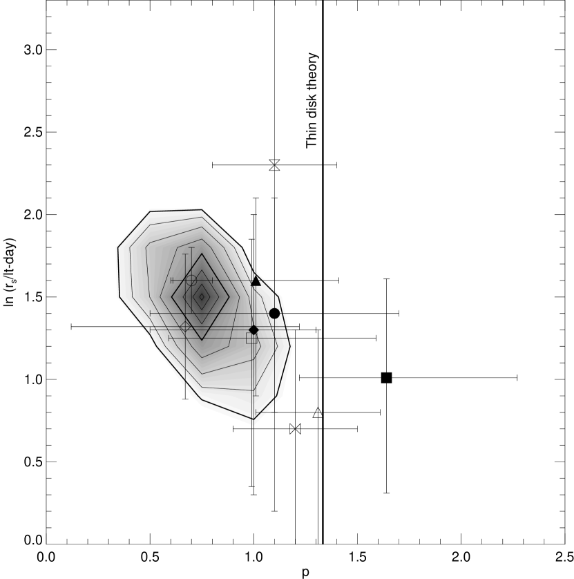
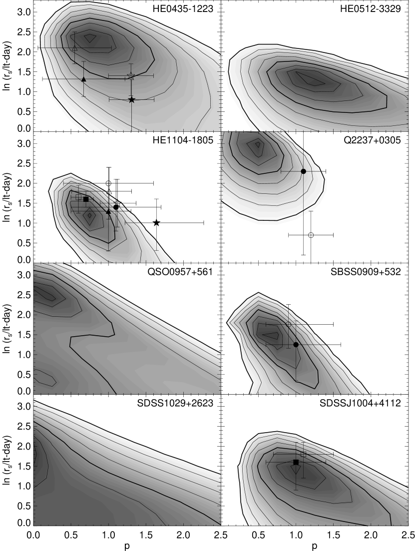
The individual likelihood distributions for each of the 8 objects are shown in Figure 1. For the case of HE1104$-$1805, where there is data at two different epochs, the distribution is the product of the probability distributions for the two epochs. Q2237+0305 combines the results for the three independent pairs at six different epochs (see Muñoz et al. 2014). In Figure 1 we also show the results from previous studies. In order to make this comparison, these sizes from the literature have, as necessary, been converted to a Gaussian $r_{s}$ at our nominal wavelength of 1026 Å  using the reported values of $p$, a microlens mass of $M=1M_{\sun}$, and assuming a fixed half-light radius, because estimates of the half-light radius are largely model independent (Mortonson et al. 2005). The general agreement is very good, with our results being compatible with previous estimates given the uncertainties. The maximum likelihood and Bayesian estimates for the size of the accretion disk $r_{s}$ at the reference wavelength (1026 Å) and for the chromaticity exponent $p$ are given in Table 2. Figure 2 shows the resulting joint likelihood. Previous estimates are also shown, although only for estimates using logarithmic priors on size to avoid overcrowding. Again, the general agreement is very good. The maximum likelihood estimates are $p=0.75^{+0.2}_{-0.2}$ and $\ln(r_{s}/\mathrm{lt-day})=1.5^{+0.3}_{-0.3}$, where these are 1$\sigma$ confidence intervals for 1 parameter. This corresponds to a size of $r_{s}(1026\ {\mathrm{\AA}})=4.5^{+1.5}_{-1.2}$ lt-days for a microlens mass of 1 $M_{\sun}$. We repeated the calculations using only the objects with spectroscopic data (i.e. excluding HE0435$-$1223 and Q2237+0305) to check whether including narrowband photometry introduces any bias, but the results are nearly identical. The most noticeable effect is that, without these objects (mostly due to the effect of Q2237+0305), the distribution is slightly more extended towards larger values of $p$ and smaller sizes. The upper limit on $p$ increases by a small amount, resulting in an estimate of $p=0.75^{+0.3}_{-0.2}$. In order to compare the present result for the size with recent estimates, we convert it to a reference wavelength of 1736 Å (using $p=0.75$) and for a mass of the microlenses of 0.3 $M_{\sun}$. The resulting (average) accretion disk size is $3.7^{+1.2}_{-1.0}$ lt-days, which is in good agreement with the value of $4.0$ lt-days estimated by Jiménez-Vicente et al. (2012) from microlensing of (basically) this lens sample without chromatic information.

The result for the size is, however, an average value for objects which, in principle, must have a spread in their sizes due to differences in their black hole masses. In order to minimize this effect when combining the likelihoods of different objects, we repeated the calculations scaling the reference size of the disk as

$$r_{s}(M_{BH})=r_{0}\left(\frac{M_{BH}}{10^{9}M_{\sun}}\right)^{2/3}$$ (4)

The 2/3 exponent is expected for Shakura & Sunyaev disks radiating close to the Eddington limit, and Morgan et al. (2010) used microlensing to estimate this scaling with mass and found results consistent with the theoretical prediction. The black hole mass estimates are based on source luminosities and emission line widths. We use estimates from the literature as reported in Table 2, using the $\mathrm{H}\beta$ estimates where available. Generally, these black hole mass estimates are viewed as logarithmically reliable with uncertainties of factors of 2-3. The resulting joint likelihood for the parameters $\ln(r_{0})$ and $p$ is shown in Figure 3.

Figure 3: Joint likelihood function for the size of the accretion disk at $M_{BH}=10^{9}M_{\sun}$, ${\ln}(r_{0}/\mathrm{lt-days})$, and the logarithmic slope, $p$, of its scaling with wavelength ($r_{s}\propto\lambda^{p}$). The contour levels are drawn at intervals of 0.25$\sigma$ as in Fig. 1. The vertical line indicates the prediction of the standard thin disk model, $p=4/3$.

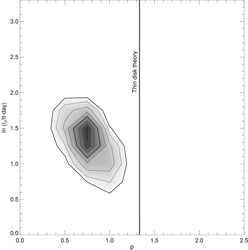
The maximum likelihood value is $\ln(r_{0})=1.5^{+0.15}_{-0.45}$, corresponding to $r_{0}=4.5^{+0.7}_{-1.6}$ lt-days which is very similar to our previous result. This was to be expected, as the average black hole mass for this sample is $1.2\times 10^{9}M_{\sun}$, which is very close to the nominal mass used in the scaling. If we assume a typical value of $0.3M_{\sun}$ for the mass of the microlenses, our estimate for the size of the accretion disk for a nominal black hole mass of $10^{9}M_{\sun}$ is very similar to the estimate by Morgan et al. (2010). The estimate of the logarithmic slope $p$ did not change, remaining at $p=0.75^{+0.2}_{-0.2}$.

On scales of $r_{0}$, we would not expect a strong object dependence of the value of $p$ for objects sharing the same emission mechanism. In spite of this, there is no general agreement on the value of $p$ from previous studies. Most earlier determinations for individual objects seemed to point near the canonical value of $p=4/3$ (e.g. Eigenbrod et al., 2008, Poindexter et al. 2008, Floyd et al., 2009, Mosquera et al., 2011), with the notable exception of the sample analyzed by Blackburne et al. (2011a), which produced an unexpectedly low value of $p=0.17\pm 0.15$ that is essentially compatible with a disk size that is independent of wavelength. Nevertheless, several recent estimates based on different techniques (Muñoz et al., 2011, Mediavilla et al., 2011, Motta et al., 2012, Blackburne et al. 2013) have been finding values close to $p=1$, although with uncertainties large enough to be consistent with the canonical value of $p=4/3$.

Figure 4: Marginalized probability distribution for the dependence of disk size on wavelength $p$ ($r\propto\lambda^{p}$). The vertical line indicates the prediction of the thin disk standard model $p=4/3$.

Figure 4 shows the Bayesian estimate of $p$ found for our sample after marginalizing over $\ln(r_{0})$. We find $p=0.8\pm 0.2$, with the value of the standard thin disk model ($p=4/3$) being excluded at the 98% confidence level. The significance drops to 90% when objects with only narrow band data are excluded.

4 Conclusions

We have used microlensing measurements for 10 image pairs from 8 lensed quasars to study the structure of their accretion disks. By using spectroscopic and narrow band photometric data we can eliminate the effects of differential extinction, which can be mistaken with chromatic microlensing and minimize any contamination from the weakly microlensed emission lines that can reduce the microlensing amplitude and potentially alter its dependence on wavelength. We find a best estimate of the wavelength dependence of the accretion disk size of $p=0.75^{+0.2}_{-0.2}$ for a maximum likelihood analysis, and $p=0.8\pm 0.2$ for a Bayesian analysis ($r_{s}\propto\lambda^{p}$). This estimate is significantly smaller than the $p=4/3$ value predicted by the Shakura & Sunyaev (1973) thin disk model with a temperature profile of $T\propto r^{-3/4}\propto r^{-1/p}$. Thus, our result seems to indicate a steeper temperature profile for the accretion disk.

Agol & Krolik (2000) proposed a model in which the magnetic connection between the black hole and the disk is able to spin the disk up leading to a steeper temperature profile with $p=8/7$, which is more consistent with our results. Another alternative is that there is some other structure on top of the accretion disk. Along this line, Abolmasov & Shakura (2012), proposed that super Eddington accretion in the disks of quasars would generate an optically thick spherical envelope that could explain the lower values of the exponent $p$ found by Blackburne et al. (2011a), although they need an ad-hoc mechanism to explain the small sizes of the X-ray-emitting regions of microlensed quasars. Note, however, that Dai et al. (2010) find that the scattered light fraction has to be very high ($\gtrsim 50\%$) before microlensing size estimates are significantly shifted by scattering. Abolmasov & Shakura (2012) proposed that this mechanism would only work for the quasars with lower black hole masses, although we do not find any trend of the parameter $p$ with the mass of the black hole. In this line, Fukue & Iino (2010) found that a fully thermalized relativistic spherical wind around the black hole would show a profile of the type $T(R)\propto R^{-1}$ which is very similar to the produced by our analysis. Note that such steeper temperature profiles make it more difficult to reconcile the larger disk sizes found by microlensing. Solutions to this problem would favor shallower profiles closer to a strongly irradiated disk with $p=2$ (see the discussion in Morgan et al., 2010). Our estimate for the size of the accretion disk of $r_{s}=4.5$ lt-days (at 1026 Å  in the rest frame) is in agreement with other recent determinations and considerably larger than the expected value from a thin disk radiating as a black body.

The large slope of the temperature profile of quasar accretion disks estimated in this work makes the already serious problem posed by the large sizes determined by microlensing for these objects even worse. As scattering does not seem to be the answer to this discrepancy, and other suitable theoretical models are lacking, evidence seems to indicate that some key ingredient in the emission mechanism of accretion disks in these objects may be missing in our present understanding. On the observational side, optical/infrared spectroscopy (or even better spectroscopic monitoring) for a larger sample of lensed quasars would be desirable to unambiguously confirm the large sizes and slopes of the temperature profile of quasar accretion disks. In the meantime, on the theoretical front, a thorough revision of the standard model of accretion disks in quasars may also be necessary.

References

- Abajas et al. (2002) Abajas, C., Mediavilla, E., Muñoz, J. A., Popović, L. C̆. & Oscoz, A. 2002, ApJ, 576, 640
- Abolmasov & Shakura (2012) Abolmasov, P. & Shakura, N. I. 2012, MNRAS, 427, 1867
- Agol & Krolik (2000) Agol, E. & Krolik J., 1999, ApJ, 524, 49
- Agol et al. (2009) Agol, E., Gogarten, S. M., Gorjian, V., & Kimball, A. 2009, ApJ, 697, 1010
- Anguita et al. (2008) Anguita, T., Schmidt, R. W., Turner, E. L. et al. 2008, A&A, 480, 327
- Assef et al. (2011) Assef, R. J., Denney, K. D., Kochanek, C. S. et al. 2011, ApJ, 742:93
- Bate et al. (2008) Bate, N. F., Floyd, D. J. E., Webster, R. L. & Wyithe, J. S. B. 2008, MNRAS, 391, 1955
- Blackburne et al. (2011a) Blackburne, J. A., Pooley, D, Rappaport, S. & Schechter, P. L. 2011a, ApJ, 729, 34
- Blackburne et al. (2011b) Blackburne, J. A., Kochanek, C. S., Chen, B., Dai, X., Chartas, G. 2011b, arXiv:1112.0027v1
- Blackburne et al. (2013) Blackburne, J. A., Kochanek, C. S., Chen, B., Dai, X., Chartas, G. 2013, arXiv:1304.1620
- Dai et al. (2010) Dai, X., Kochanek, C. S., Chartas, G. et al. 2010, ApJ, 709, 278
- Eigenbrod et al. (2008) Eigenbrod, A., Courbin, F., Meylan, G. et al. 2008, A&A, 490, 933
- Falco et al. (1999) Falco, E. E., Impey, C. D., Kochanek, C. S. et al. 1999, ApJ, 523, 617
- Floyd et al. (2009) Floyd, D. J. E., Bate, N. F., & Webster, R. L. 2009, MNRAS, 398, 233
- Fukue & Iino (2010) Fukue, J. & Iino, E. 2010, PASJ, 62, 1399
- Guerras et al. (2013a) Guerras, E., Mediavilla, E., & Jiménez-Vicente, J. et al. 2013a, ApJ, 764, 160
- Guerras et al. (2013b) Guerras, E., Mediavilla, E., & Jiménez-Vicente, J. et al. 2013b, ApJ, 778, 123
- Hainline et al. (2012) Hainline L. J., Morgan C. W., Beach J. N. et al. 2012, ApJ, 744, 104
- Jiménez-Vicente et al. (2012) Jiménez-Vicente, J., Mediavilla, E., Muñoz, J. A., & Kochanek, C. S. 2012, ApJ, 751, 106
- Kochaneck (2004) Kochanek, C. S. 2004, ApJ, 605, 58
- Maoz et al. (1993) Maoz, D. et al. 1993, ApJ, 404, 576
- Mediavilla et al. (2006) Mediavilla, E., Muñoz, J. A., Lopez, P., et al. 2006, ApJ, 653, 942
- Mediavilla et al. (2009) Mediavilla, E., Muñoz, J. A., Falco, E., et al. 2009, ApJ, 706, 1451
- Mediavilla et al. (2011a) Mediavilla, E., Muñoz, J. A., Kochanek, C. S., et al. 2011a, ApJ, 730, 16
- Mediavilla et al. (2011b) Mediavilla, E., Mediavilla, T., Muñoz, J. A. et al. 2011b, ApJ, 741, 42
- Minezaki et al. (2009) Minezaki, T., Chiba, M., Kashikawa, N., Inoue, K. T., & Kataza, H. 2009, ApJ, 697, 610
- Morgan et al. (2008) Morgan, C. W., Kochanek, C. S., Dai, X., Morgan, N. D., & Falco, E. E. 2008, ApJ, 689, 755
- Morgan et al. (2010) Morgan, C. W., Kochanek, C. W., Morgan N. D. & Falco E. E. 2010, ApJ, 712, 1129
- Mortonson et al. (2005) Mortonson, M. J., Schechter, P. L. & Wambsganss, J. 2005, ApJ, 628, 594
- Mosquera et al. (2009) Mosquera, A. M., Muñoz, J. A., & Mediavilla, E. 2009, ApJ, 691, 1292
- Mosquera et al. (2011) Mosquera, A. M., Muñoz, J. A., Mediavilla, E., Kochanek, C. S. 2011, ApJ,728, 145
- Mosquera et al. (2013) Mosquera, A. M., Kochanek, C. S., Chen, B. et al. 2013, ApJ, 769, 53
- Motta et al. (2012) Motta, V., Mediavilla, E., Falco, E., & Muñoz, J. A. 2012, ApJ, 755, 82
- Muñoz et al. (2004) Muñoz, J. A., Falco, E. E., Kochanek, C. S., McLeod, B. A., & Mediavilla, E. 2004, ApJ, 605, 614
- Muñoz et al. (2011) Muñoz, J. A., Mediavilla, E., Kochanek, C. S., Falco, E. E. & Mosquera, A. M. 2011, ApJ, 742, 67
- Muñoz et al. (2014) Muñoz, J. A., et al. 2014, in preparation
- Novikov & Thorne (1973) Novikov, I. D. & Thorne, K. S. 1973, in Black Holes, ed. C. De Witt & B. De Witt (New York: Gordon & Breach), 343
- Peng et al. (2006) Peng, C. Y., Impey, C. D., Rix, H. W. et al. 2006, ApJ, 649, 616
- Poindexter et al. (2008) Poindexter, S., Morgan, N. & Kochanek, C. S. 2008, ApJ, 673, 34
- Poindexter & Kochanek (2010) Poindexter, S. & Kochanek, C. S. 2010, ApJ, 712, 668
- Pooley et al. (2007) Pooley, D., Blackburne, J. A., Rappaport, S., & Schechter, P. L. 2007, ApJ, 661, 19
- Shakura & Sunyaev (1973) Shakura, N. I. & Sunyaev, R. A. 1973, A&A, 24, 337
- Wambsganss (2006) Wambsganss, J. 2006, Gravitational Lensing: Strong, Weak, and Micro, ed. G. Meylan, P. North, & P. Jetzer (Berlin: Springer), 453
- Wills, Netzer & Wills (1985) Wills, B. J.; Netzer, H.; Wills, D. 1985, ApJ, 288, 94
- Wucknitz et al. (2003) Wucknitz, O., Wisotzki, L., Lopez, S., & Gregg, M. D. 2003, A&A, 405, 445