The ”sugar” coarse-grained DNA model

Abstract

More than twenty coarse-grained (CG) DNA models have been developed for simulating the behavior of this molecule under various conditions, including those required for nanotechnology. However, none of these models reproduces the DNA polymorphism associated with conformational changes in the ribose rings of the DNA backbone. These changes make an essential contribution to the DNA local deformability and provide the possibility of the transition of the DNA double helix from the B-form to the A-form during interactions with biological molecules. We propose a CG representation of the ribose conformational flexibility. We substantiate the choice of the CG sites (6 per nucleotide) needed for the ”sugar” GC DNA model, and obtain the potentials of the CG interactions between the sites by the ”bottom-up” approach using the all-atom AMBER force field. We show that the representation of the ribose flexibility requires one non-harmonic and one three-particle potential, the forms of both the potentials being different from the ones generally used. The model also includes (i) explicit representation of ions (in an implicit solvent) and (ii) sequence dependence. With these features, the sugar CG DNA model reproduces (with the same parameters) both the B- and A- stable forms under corresponding conditions and demonstrates both the A to B and the B to A phase transitions.

I Introduction

The local DNA deformability is crucial for the DNA biological functioning: winding around histones (unwrapping and rewrapping), interactions with proteins, transcription and replication. The deformation of the double helix is mostly achieved through three types of mobility in the DNA backbone: concerted change of torsion angles $\alpha$ and $\gamma$ Varnai et al. (2002); $\zeta$ and $\varepsilon$ Hartmann et al. (1993) (for notations, see fig. 2); and ribose flexibility (the change of conformation of the sugar rings). The last mentioned type makes an essential contribution into providing the observed extreme deformability.

The local changes of sugar conformations are very common in physiological saline. In vivo, they take place in the binding of some proteins (such as TBP, SRY, LEF-1, PurR) to the minor groove of the (common) B form of double stranded DNA (dsDNA). During this process, the minor groove widens through transitions of several sugar rings into conformations characteristic for the A-form of dsDNA Lebrun and Lavery (1999); Olson and Zhurkin (2000). Many local B to A conversions have been observed in protein and drug-bound DNA crystal complexes Lu et al. (2000). Particularly, such conversion takes place when an enzyme interacts with the atoms ordinarily buried within the backbone (O3’, for example). Generally, a dsDNA can assume an A-form structure when the properties of the solution and/or the amount and/or type of ions near its surface change, as well as during interaction with the partial charges on the surfaces of biomolecules. The geometric shape of the A-DNA differs from that of the B-DNA, and the mechanical properties of these helices are also different. One can obtain DNA crystals from a solution in both the A- and B-forms depending on salt concentration, relative humidity and base pairs sequenceArnott (2006). In a solution, one can induce a B to A transition by increasing salt concentration and/or adding ethanol to the solvent Ivanov et al. (1973); Nishimura et al. (1986). The ethanol concentration, at which the B to A transition occurs, depends on the nucleotide sequence Ivanov and Krylov (1992): more C:G pairs shift the transition to smaller ethanol concentrations. It should be noted that other characteristics of a DNA nucleotide (both structural and dynamical ones) also depend on its base and a few neighboring bases.

Therefore, the geometry (and, as a consequence, mechanical and dynamical properties) of both the A-DNA and B-DNA forms is a result of a complex balance of interdependent factors: torsion angles in the backbone; ribose conformations; sequence dependent base pair stacking and pairing; electrostatic interactions of DNA with solvent molecules and with salt ions. From the physical point of view, the understanding of this balance is equivalent to the construction of a coarse-grained (CG) DNA model able to reproduce the needed features of the DNA behavior.

The last fifteen years witnessed the extensive development of CG models for different substances Karimi-Varzaneh and Muller-Plathe (2012), particularly for large biomolecules Takada (2012); Noid (2013a). A series of regular methods for obtaining CG force fields have been developed Brini et al. (2013); Noid (2013b). However, the regular methods imply that the potentials are pairwise and/or have a given simple form. As we will show later, if the objective is to model the effect of the ribose flexibility on the DNA geometry, one has to use one non-harmonic and one three-particle potential, both of the form different from the potentials generally used.

Because of the complexity of the behavior of the DNA molecule and because of the different needed level of detail in various physical situations, more than 20 CG DNA models have already been developed. There are several good reviews of these models Sim et al. (2012); Potoyan et al. (2013); Dans et al. (2016); Korolev et al. (2016), we will only describe one trend in their evolution.

To reproduce the properties common to dsDNA and other semiflexible polymers, one can use the simplest worm-like chain model with a bead consisting of two complementary nucleotides Wang and Gao (2005). Similar models are being exploited in extensive simulations of long DNA molecules, for example, in the analysis of the behavior of a dsDNA confined in a nanochannel Cifra et al. (2009); Wang et al. (2011); Muralidhar et al. (2014) or in simulation of single stranded DNA molecules (ssDNA) in DNA-functionalized spherical colloids Theodorakis et al. (2013). In this model, one usually obtains the model parameters from comparison with the experimental data (”top-down” approach). A modification of this model Mazur (2009) allows one to obtain both bending and torsional persistent lengths (consistent with experiment). However, the modified model gives one order of magnitude lower value for the relaxation rate of bending fluctuations Mazur (2009). The reason is that the DNA bending is more sophisticated than in the worm-like model because on the scale less than 100nm the dsDNA behaves rather like a stack of interacting plain nucleobases Becker and Everaers (2007). The models including plain bases can represent the local inner dynamics of the molecule more adequately, and these models are able to take into account the sequence dependence Coleman et al. (2003); Mergell et al. (2003); Becker and Everaers (2007). To derive the potentials of interactions between the bases, one can use the results of classical all-atom simulations or quantum chemical calculations (”bottom-up” approach) Andrews et al. (2010); Maciejczyk et al. (2010); Hsu et al. (2012).

To simulate the dsDNA denaturation and hybridization (as well as transcription or replication), one needs at least two interacting chains of beads. The simplest approach is to use one interaction site per nucleotide. Depending on the intended application, interchain (interstrand) interactions can have different levels of complexity: a bead on one chain may interact with one Kim et al. (2008), three Jeon and Sung (2014); Doi et al. (2010) or many beads Savelyev and Papoian (2009a); Naômé et al. (2014) on the second chain. The models of this type are able to reproduce the geometrical shape of B-DNA, and, together with explicitly modelled ions, the dependence of the persistence length on the ionic concentration Korolev et al. (2016). These models allow to develop the regular methods for obtaining the interaction potentials between the beads: molecular renormalization group coarse-graining Savelyev and Papoian (2009a), newton inversion method Naômé et al. (2014). However, to simultaneously simulate, on the one hand, the correct geometry and mechanics, and, on the other hand, the adequate possibility for splitting into two strands, one needs, at least, one interaction site for the nucleobase and, at least, one interaction site for the backbone part of the nucleotide Ouldridge et al. (2010); Maffeo et al. (2014). With the proper interactions between the bases, this model is elaborate enough for simulation of DNA melting, hairpin formation and duplex hybridization Ouldridge et al. (2011), as well as the sequence dependence Šulc et al. (2012). However, the dynamics of the molecule backbone is better modelled if one uses two sites on the backbone per nucleotide: one for the phosphate group and one for the sugar. The number of sites on the base also may be chosen to be more than one to better describe stacking and pairing. Actually, most of the CG DNA models are of this type Drukker et al. (2001); Tepper and Voth (2005); Knotts IV et al. (2007); Morriss-Andrews et al. (2010); Linak et al. (2011); Maciejczyk et al. (2014); Markegard et al. (2015). For a model of this type, a force field for DNA-protein interactions has been offered Yin et al. (2015).

To deal with the same problem of the protein-DNA docking, another model of CG DNA has been elaborated Poulain et al. (2008) for the CG proteins earlier offered Zacharias (2003). In this model, the third interaction site on the backbone part of the nucleotide was introduced (the ribose ring is divided into two beads). This CG model well reproduces the geometry of some protein-DNA complexes, and so it seems that the shape of the CG strands is fine enough to model the needed large local deformations of the dsDNA in the complexes. The model with the same number of beads on the backbone Dans et al. (2010) can well reproduce the dsDNA breathing dynamics (and melting) and its dependence on sequence specificity. However, the natural question arises: are these strands flexible enough if the potentials of interactions between the beads do not allow to simulate the conformational changes in the ribose rings, whereas the ribose flexibility significantly contributes to the flexibility of the strands?

We think that the answer is ’no’. To adequately reproduce DNA local deformability, the model needs to reproduce the ribose flexibility. It means that both the B- and A-DNA forms and the transitions between them should be present at the corresponding physical conditions. In this article, we propose the first CG model meeting this requirement. More precisely, using all-atom simulations and experimental data, we justify the choice of beads on the backbone (their minimal needed number and location) and the potentials of interactions between them. We show that the existence of the A-DNA can be provided only if the ions are treated explicitly. For the derivation of the model, we exploit the interactions between bases as in the AMBER force field, but the proposed method of introducing ribose flexibility may be used with any of the CG base interactions obtained by ”bottom-up” approach Andrews et al. (2010); Maciejczyk et al. (2010); Hsu et al. (2012).

We formulated the choice of the beads and derived the potentials for simulating ribose flexibility in 2010 Kikot et al. (2010). The version of the model without implementation of the ribose flexibility, without the sequence dependence, and with implicit solvent (generalized Born approximation with the Debye-Huckel correction for salt effects Srinivasan et al. (1999)) has been used for estimation of the B-DNA heat conductivity Savin et al. (2011) and for investigation of dsDNA stretching Savin et al. (2013). However, this version is admissible only when one may neglect the ribose flexibility (under low temperatures or when the molecule can be extended but not bent and not compressed). At temperature 300 K, the behaviour of this CG B-DNA and the all atom AMBER model significantly differ Kikot et al. (2011). Here, we present the full model (hereinafter referred to as the ”sugar” CG DNA model), including explicit representation of ions and sequence dependence. The parameters of the model are accurately adjusted, so that it can simulate both B- and A-DNA at proper conditions, and demonstrates both the A to B and the B to A transitions.

II Model construction

For base pairs stacking and pairing, we accept the AMBER force field Parm99SB+bsc0 Wang et al. (2000); Hornak et al. (2006); Perez et al. (2007). This choice is justifiable, considering that the empirical force fields reproduce the forces acting between bases better than any other forces in the DNA molecule Sponer et al. (2006). We analyze the dsDNA dynamics in solvents at 300 K in the framework of the all-atom AMBER model (for B-DNA in water - Parm99SB+bsc0, for A-DNA in the mixture of ethanol and water (85:15) - Parm99 (we used the trajectory obtained )). Besides, we analyze the geometric changes of the dsDNA helix at A-B transition and at base-pair opening. On the basis of these data, we divide the DNA strands into ”beads” and find the potentials for interactions between the beads. We obtain the potentials describing the ribose flexibility from the AMBER force field (Parm99SB+bsc0) using the ”bottom-up” approach. Finally, we choose the description of the medium: the models for the ions and the solvent.

II.1 Beads on nucleobases, stacking and pairing

We model a base as three rigidly bound beads which can rotate around an axis coinciding with the real rotation axis of the base: the glycosidic bond $\chi$. We placed the beads on some (heavy) atoms of the bases (see fig. 2).

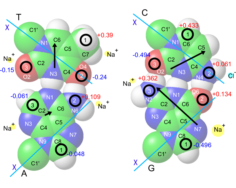
Figure 1: Coarse graining of the natural base pairs (A:T and G:C). We show the locations and and the charges of three rigidly bound beads modeling every base. The rotation axes (glycosidic bonds $\chi$ with the sugar rings) are marked. We use common designations for DNA atoms Neidle (2008), and we depict their van-der-Waals radii. The black arrows present electric dipole moments of the bases (according to the charge distribution in AMBER), and the circles near atoms of the bases - zones around A-DNA where one can find ions Na⁺ or Cl^- with maximal probability Feig and Pettitt (1999).

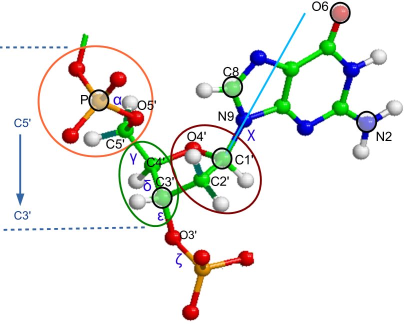
Figure 2: Coarse graining of the sugar-phosphate backbone. We show locations of the beads and (for the backbone) the groups of atoms united into the beads. We use common notations for the atoms and torsion angles Neidle (2008). A nucleobase rotates about the glycosidic bond $\chi$.

One of the atoms was chosen on one side of the rotation axis, the two others - on the other side, at maximum distance from the center of the base. The objective of this choice was to best approximate the real moments of inertia of the base. For base A (Adenine) we placed the beads on atoms C8, N6, C2; for base T (Thymine) - on atoms C7, O4, O2; for base G (Guanine) - on atoms C8, O6, N2; and for base C (Cytosine) - on atoms C6, N4, O2 (see fig. 2). Masses of the beads $m_{1}$, $m_{2}$, $m_{3}$ on a base X (X = A, T, G, C) were found from the two conditions: (1) equality of the total mass of the beads to the mass of the base ($m_{1}+m_{2}+m_{3}=m_{X}$) and (2) coincidence of the mass centers of the three beads and the base. Numerical values for masses of beads and moments of inertia of the CG and real bases are given in table 1.

Table 1: Masses of beads $m_{1}$, $m_{2}$, $m_{3}$ and moments of inertia of the real i_xx and i_yy and the CG I_xx and I_yy bases A, T, G, C. Masses of the beads are given in a.e.m., the moments of inertia - in a.e.m.$\cdot\mbox{\AA}^{2}$.

X	$m_{1}$	$m_{2}$	$m_{3}$	ixx	Ixx	iyy	Iyy
A	$52.230$	$28.139$	$53.632$	$690$	$475$	$1704$	$1712$
T	$51.822$	$16.204$	$56.974$	$584$	$256$	$1636$	$1543$
G	$61.731$	$34.357$	$53.912$	$1302$	$800$	$1885$	$1858$
C	$39.254$	$35.492$	$35.254$	$233$	$164$	$1344$	$1231$

Knowing the coordinates of the three beads, one can find the coordinates of all the base atoms and compute the energy of base pairing and base stacking as the sum of pairwise atomic electrostatic and van-der-Waals interactions. For them, we used the AMBER force field (Parm99SB+bsc0 Wang et al. (2000); Hornak et al. (2006); Perez et al. (2007)). Savin et al Savin et al. (2011, 2013) used the partial interaction between the bases to decrease the computation time. In the present realization of the model, every atom of a base interacts with every atom of the complementary base and with all the atoms of two neighboring base pairs. It allows to simulate the A-DNA form and other deformed structures (for example, base pair opening).

The accepted interactions between bases are computationally expensive (as compared to the other interactions in the CG model). We used them only as a foundation to construct the adequate CG backbone and test the obtained structure. If one uses the sugar CG model in long simulations of biological processes in the future, the described scheme should be replaced with a CG one (derived by ”bottom-up” approach Andrews et al. (2010); Maciejczyk et al. (2010); Hsu et al. (2012)).

II.2 Beads on backbone

We choose the locations of all the beads on (heavy) atoms. The main principle was: one may distort the mass distribution of the molecule, but one preserves its key geometric nodes. We will show that, to achieve this, one needs three beads per nucleotide for the backbone (see fig. 2 ).

The first bead was chosen on atom C1’ because it is the point of suspension of the base, and the rotation axis of the base (glycosidic bond) passes through this atom. Crystallographic data Gelbin et al. (1996) show that bases rotate around this axis considerably, while valence angles O4’C1’N1(N9) and C2’C1’N1(N9) practically do not change and fix the direction of the glycosidic bond relative to the ribose ring. This is the key geometric peculiarity of the connection between a base and the backbone, and we keep this peculiarity in our model.

The second bead was chosen on phosphorus atom, and united phosphate group and three atoms (C5’, H5’1, H5’2) which normally move together with the phosphate Bruant et al. (1999). As we want to minimize the number of beads per nucleotide, we would tend to restrict the backbone to the chain (…-P-C1’-P-C1’-…). However, all atom MD simulations show that the presence of the very flexible sugar rings between the atoms P and C1’ allows the dihedral angles in this chain to vary over a very wide range, while the dihedral angles in the chain (…-P-P-P-…) keep their mean values quite satisfactorily. To preserve this feature, we need at least one more bead per nucleotide. Besides, we would like to build a backbone which can serve as a support for the moving bases at their opening and in A-B transition (which is the case for the real sugar-phosphate backbone of DNA). This purpose is also not achieved for the chain (…-P-C1’-P-C1’-…) as the atoms C1’ always move together with the bases.

When a ribose ring changes its conformation, the torsion angles around the bonds adjoining the ring also change, and so does the position of the ring relative to the two neighboring phosphate groups, as well as the distance between the groups. The adjacent base pairs move relative to each other, and the local geometry changes from B-like to A-like (see fig. 3).

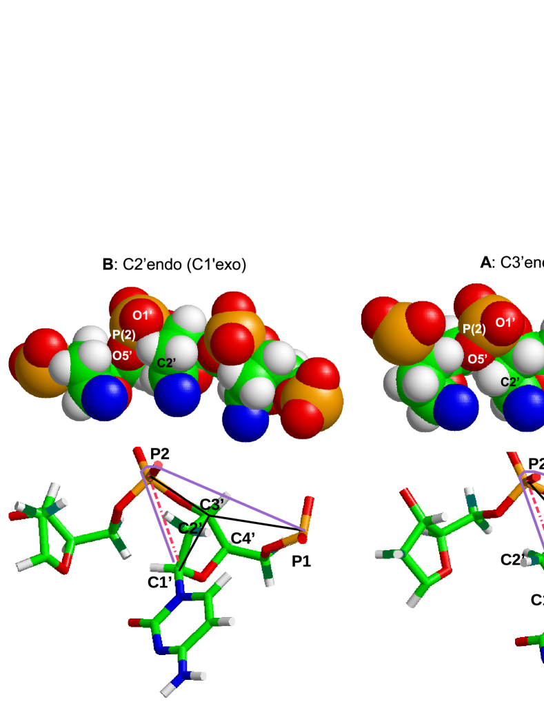
Figure 3: CG model of the ribose flexibility. The valence bonds and angles, on the one hand, and the van-der-Waals interactions, on the other hand, provide two stable positions of the ring relative to the phosphates exactly when the ring has C2’-endo (B-DNA) and C3’-endo (A-DNA) conformations: between two phosphates and under the chain of phosphates. Intermediate positions suffer strong steric hindrance, which results in a barrier between these two energy minima. When the ring changes its conformation, it has to change its position relative to the chain of phosphates (distance C1’P(2)). This, in turn, has to change the distance between the phosphates. So we have correlations: (C2’-endo $\rightleftharpoons$ small $\mid$C1’P(2)$\mid$ $\rightleftharpoons$ large $\mid$P(1)P(2)$\mid$ $\rightleftharpoons$ B-DNA) and (C3’-endo $\rightleftharpoons$ large $\mid$C1’P(2)$\mid$ $\rightleftharpoons$ small $\mid$P(1)P(2)$\mid$ $\rightleftharpoons$ A-DNA). Therefore, we choose sufficiently rigid harmonic potentials for the CG bonds C3’-P(2), P(1)-C3’ and C3’-C1’. For the CG bond C1’-P(2), we introduce a double-well potential. The two wells correspond to two main conformations of the sugar ring. The correlation of the distance $\mid$P(1)P(2)$\mid$ with $\mid$C1’P(2)$\mid$ is described by potential (1). This potential can be symbolically depicted as one spring thrown from bead P(1) to bead C1’ over bead P(2). For the long CG bond P(1)-C1’, we use a soft spring.

One can see that the atom C4’ moves with the sugar ring when its conformation changes. On the contrary, the displacement of the atom C3’ is mostly caused by the necessity to change the geometric form of the chain of phosphates. Therefore, we choose the third bead on the atom C3’.

As a result, to hold the needed form of the DNA strand, we use CG bonds, CG angles, and CG dihedral angles in the chain of beads (…-P-C3’-P-C3’-…). To model the ribose flexibility, we add beads C1’ (connected to bases) attached to the C3’ beads of this chain. The position of the CG bond C3’-C1’ relative to the chain (…-P-C3’-P-C3’-…) should have two locations divided by a barrier - which reflects two main states of the ribose.

II.3 Ribose flexibility

Ribose flexibility is modeled via double-well potential for CG bond C1’-P(2) - see fig. 3. The all atom simulations also show that it is this bond of all the distances in the CG pyramid {P(1)P(2)C3’C1’} that directly correlates with the ribose conformation (see fig. (S1) in Supplemental Material Sup ). The correlation between the distances $\mid$P(1)P(2)$\mid$ and $\mid$C1’P(2)$\mid$ is introduced via three-particle potential

$$U=\frac{1}{2}k_{P}(\left|P(1)P(2)\right|+t_{P}\left|C1^{\prime}P(2)\right|-l_{P0})^{2},$$ (1)

where $t_{P}>0.$ From direct geometric considerations, one could also expect a (positive) correlation between distances $\mid$P(1)C1’$\mid$ and $\mid$C1’P(2)$\mid$. However, as we will see from the all-atom simulations, one can use a soft harmonic potential for this CG bond: the distance $\mid$P(1)C1’$\mid$ does not directly correlate with the sugar conformation. Indeed, there are five valence bonds and three torsion angles between atoms P(1) and C1’, and these degrees of freedom are only weakly connected with the sugar conformation.

II.4 Obtaining parameters of CG potentials from all-atom modeling

To derive the potentials for the CG bonds and angles (fig.4), we used two methods. We estimated the rigidities of harmonic bonded potentials (CG bonds, CG angles, CG dihedral angles) by the simplest Boltzmann inversion method Tschop et al. (1998) for all-atom MD trajectories of a B-form of dsDNA in water (AMBER, Parm99SB+bsc0 Wang et al. (2000); Hornak et al. (2006); Perez et al. (2007)) and an A-form of dsDNA in the mixture of ethanol and water (85:15) (AMBER, Parm99, we used the trajectory obtained by A. Noy et al Noy et al. (2007)). In this approach, the obtained rigidities take into account not only the (valence, torsion and van-der-Waals) interactions between the DNA atoms, together with the DNA solvation. In addition, these rigidities partly ”include” several interactions which we plan to introduce separately: base stacking; electrostatic interactions between charges on DNA, and between charges on DNA and ions. Therefore, to verify the obtained rigidities and, in some cases, to evaluate the CG potentials which can not be derived in such a way (for example, in the case of the double-well potential for the CG bond C1’-P(2)), we used an another method (method of ”relaxation”).

Namely, to obtain the energy of interaction between two beads at a given distance, we took an all-atom fragment of one DNA strand (without charges, in vacuum) between the atoms corresponding to these beads, and located these atoms at the needed distance one from another. Then we minimized the energy of the system (in the framework of the AMBER force field Parm99SB+bsc0) as a function of coordinates of all the rest atoms (and so we carried out the ”relaxation” of the system). The obtained value of energy was regarded as the energy of interaction between the beads at this distance. Changing the distance between the beads, we obtained the dependence of the energy on the distance. In this way one can evaluate potentials of ”valence” bonds in a CG model.

The details of the derivation of the potentials are collected in Appendix A in Supplemental Material Sup . The description of the resulting force field is given in table 3.

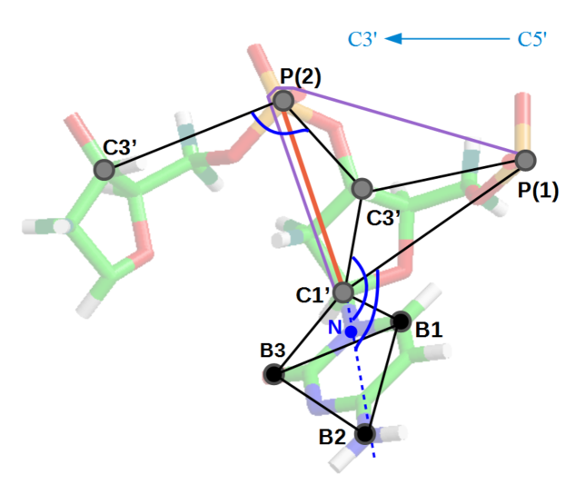
Figure 4: CG bonds and angles of the sugar CG model. The double-well bond C1’-P(2) models ribose flexibility, the length $\mid$P(1)P(2)$\mid$ correlates with the length $\mid$C1’P(2)$\mid$ (potential (1) is symbolically depicted as the polyline P(1)-P(2)-C1’). Atom N (N1 or N9) is not one of the beads of the CG model, it is shown merely to determine the direction of the glycosidic bond, around which the base rotates.

II.5 Modeling DNA environment

It is clearly seen from the all atom modeling Jayaram et al. (1998); Sprous et al. (1998) that most counter-ions are situated near the surface of the A-DNA, and almost in one thin layer. Closer examination shows that the counter-ions are located mostly in the major groove of the A-DNA both in ethanol-water mixture Cheatham III et al. (1997) and in a small water drop Mazur (2003). It allows the phosphates on the opposite sides of the major groove to approach each other, and thus forms the characteristic cavity of the A-DNA. It is obvious that such ion distribution can not be described in the framework of any implicit approach. And, indeed, if one uses the generalized Born approximation with Debye-Huckel correction for salt effects, only some shift of the DNA form from B to A can be observed when 1M of salt is added Chocholousova and Feig (2006). Contrary to this, with explicit media modeling in the framework of the CHARMM force field, the transition from B- to A-DNA took place in 1.5 nanoseconds with only 0.45M of salt added Yang and Pettitt (1996). Therefore we introduce ions explicitly.

Explicit modeling of solvent takes lion’s share of computational resources, and we know of no evidence that interaction of DNA with solvent molecules should be treated explicitly. Therefore, all the known effects of the medium (electrostatics and solvation), which may affect the balance of interactions in the system, are represented implicitly, via effective potentials of interaction between the beads of the CG model, between the ions, and between the ions and the beads of the CG model.

II.5.1 Electrostatic interaction between phosphate beads: distance dependent permittivity

The simplest way to model electrostatic forces between phosphates is to put negative charges (-$e$) on phosphate beads and to introduce the Coulomb potential of interaction between these charges. Because of the small distances between phosphates and because of the appreciable changes in the distances in B$\leftrightarrow$A transition one has to use a distance dependent permittivity $\varepsilon(r)$ in this potential. Indeed, the dielectric constant $\varepsilon$ is close to vacuum at small distances between the charges because there are not enough solvent molecules between the phosphates for screening their charges. Therefore, $\varepsilon$ is normally taken equal to 2-3 at small distances. With increasing distance $r$, $\varepsilon(r)$ is expected to reach its macroscopic value. Starting value and slope of this curve depend on size and dipole moment of solvent molecules, as well as on the location of the charges on the DNA molecule.

One may use various analytical forms for the dependence $\varepsilon(r)$ Wang et al. (2002); Mazur and Jernigan (1991). We adopted the simplest representation already used in one CG DNA model Freeman et al. (2011):

$$\varepsilon(r)=\varepsilon{{}_{0}}+\varepsilon{{}_{1}}\tanh[\exp\left(\frac{\alpha}{2}(r-r_{0})\right)],$$ (2)

with differing parameters: $\varepsilon_{0}=58$ and $\varepsilon_{1}=22$, $\alpha=12\mbox{\AA}^{-1}$, $r_{0}=8.5\mbox{\AA}$. This function is shown in fig. 5.

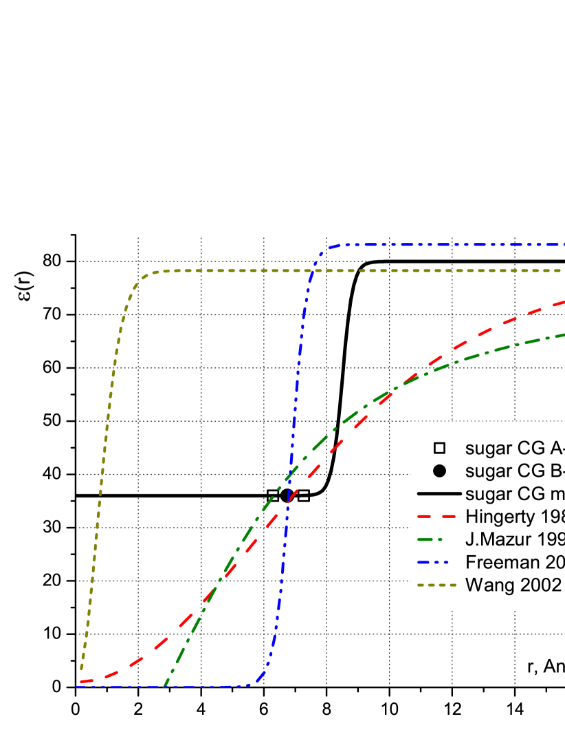
Figure 5: Screening of phosphate charges: distance dependence of permittivity $\varepsilon(r)$ in the Coulomb potential of repulsion between negative charges on phosphate beads. We compare the dependence adopted in our model with the dependencies offered or used in other works: by Hingerty et al Hingerty et al. (1985) for charges on biopolymers, by J.Mazur at al Mazur and Jernigan (1991) and by Wang et al Wang et al. (2002) for all-atom B-DNA modeling, and by Freeman et al Freeman et al. (2011) for a CG B-DNA. The points show the dielectric constants on MD trajectory of our sugar CG model for the nearest beads along the strand in A-DNA and B-DNA: $\varepsilon(6.29\mbox{\AA})=36$ and $\varepsilon(6.7\mbox{\AA})=36$, and for the nearest beads located across the major groove: $\varepsilon(7.3\mbox{\AA})=36$ (A-DNA), $\varepsilon(16.2\mbox{\AA})=80$ (B-DNA).

II.5.2 Interactions between ions, and between ions and DNA beads: solvation effects and sequence dependence

A-DNA can not be simulated in water with sodium counterions, even in a small box. The only exception we know of is in a work where a B to A transition was observed in a tiny water drop in which the surface tension contributed to the formation of the compact A-DNA Mazur (2003). Normally, one needs to add salt to a dsDNA with counterions to observe an A-DNA Yang and Pettitt (1996). Therefore, in the CG model, we included explicit ions Na⁺ and Cl^- and interactions between them, and between the ions and the charges on DNA.

We also found that the charges (-e) on phosphates (e is an elementary charge) are not sufficient for the formation of A-DNA, one needs to put partial charges on bases (on beads $B_{1}$, $B_{2}$, $B_{3}$ of all the bases), and so to introduce the sequence dependence. More exactly, the A-DNA conglomerate is not stable if there are no charges on bases keeping the sodium ions inside the major groove. Therefore, we distributed partial charges on beads (table 2) so that the dipole moment of every (neutral) base coincided with the moment in the AMBER force field (Parm99SB+bsc0 Wang et al. (2000); Hornak et al. (2006); Perez et al. (2007)).

Table 2: Charges (in units of the elementary charge e) of base beads interacting with ions in solution.

type of base	B1	B2	B3
Adenine	-0.048	0.109	-0.061
Thymine	0.390	-0.240	-0.150
Guanine	-0.496	0.134	0.362
Cytosine	0.433	0.061	-0.494

One can obtain effective potential of interaction between ions in a solvent from a radial distribution function (rdf) in an all atom simulation by several different methods Lyubartsev and Laaksonen (1999); Lyubartsev and Marčelja (2002); Hess et al. (2006); Savelyev and Papoian (2009b). These methods yield the potentials of close shapes. We chose the analytical representation of the potential function proposed by Savelyev and Papoian Savelyev and Papoian (2009b):

$$\mathcal{V}_{ij}=\frac{A}{{r_{ij}}^{12}}+\sum_{k=1}^{5}D_{k}\exp^{-C_{k}\left[r_{ij}-R_{k}\right]^{2}}+\frac{q_{i}q_{j}}{4\pi\varepsilon_{0}\varepsilon r_{ij}},$$ (3)

where $r_{ij}$ is the distance between $i$th and $j$th particles (between ions or between an ion and a DNA bead). In this expression, the first term introduces excluded volume, the second term describes the shape of peaks and minima of the potential due to solvation, and the last term is the long-distance asymptotics: electrostatic (Coulombic) interaction between the charges.

We adopted Cl^--Na⁺ and Cl^--Cl^- potentials obtained by Lyubartsev and Marčelja Lyubartsev and Marčelja (2002) from all atom simulation of 0.5M NaCl electrolyte. In the simulation the authors used the Smith-Dang’s ion model Smith and Dang (1994). Because we have few Cl^- ions interacting mostly with Na⁺ ions and one with another, we assumed that we may use these potentials, even with a dsDNA molecule added in solution. For the interactions of Cl^- ions with phosphate beads Cl^--P, we adopted the potential obtained by Lyubartsev and Laaksonen Lyubartsev and Laaksonen (1999), again from all atom simulations with the Smith-Dang’s ion model. We also used Na⁺-Na⁺, Na⁺-Cl^- and Cl^--Cl^- potentials derived by Lyubartsev and Marčelja Lyubartsev and Marčelja (2002) as templates for potentials of interaction between ions and beads on bases. We did not put any charges on the beads C1’ and C3’, and the ions interact with them only by excluded volume potential. The details of the derivation of these potentials are in Appendix B Sup .

Potentials of interaction between sodium ions and between sodium ions and phosphate beads were chosen so that there are both A-DNA and B-DNA, as well as both A$\rightarrow$B and B$\rightarrow$A transitions in the model. In figures 7 and 7 we compare these potentials with the ones obtained by different methods or exploited in some works.

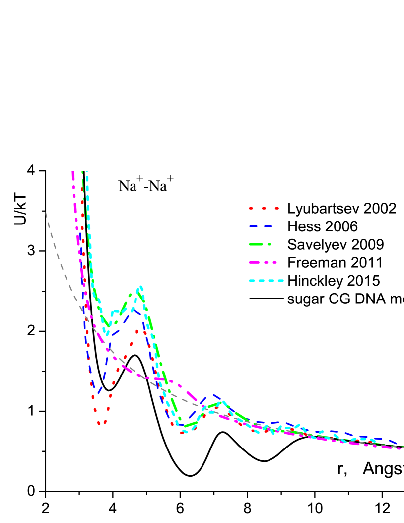
Figure 6: Comparison of effective potentials of sodium ions interaction. The solid line corresponds to the potential used in the sugar CG DNA model. We show potentials obtained by different methods from all-atom simulations of ions in aqueous solution in works by Lyubartsev et al Lyubartsev and Marčelja (2002), Hess et al Hess et al. (2006), Savelyev et al Savelyev and Papoian (2009b), Hinckley et al Hinckley and de Pablo (2015). We also show the potential used in CG modeling of B-DNA by Freeman et al Freeman et al. (2011). Thin dashed curve corresponds to the Coulombic interaction between the charges (the last term in equation (3)).

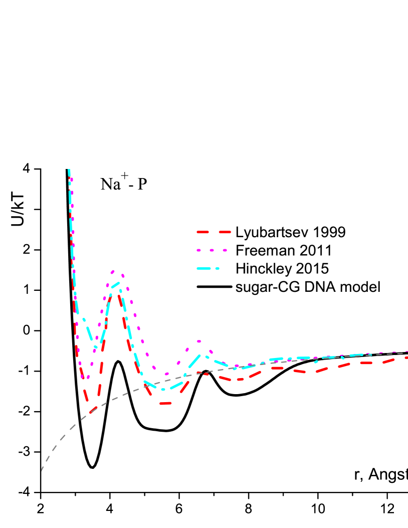
Figure 7: Comparison of effective potentials of interaction between phosphate bead and sodium ion. The potential used in the sugar CG model - solid line, the one obtained by Lyubartsev et al Lyubartsev and Laaksonen (1999) from all-atom simulation of B-DNA - dashed line; the one used in CG modeling of B-DNA by Freeman et al Freeman et al. (2011) - dotted line. Dash-dot line represents the potential obtained by Hinckley et al Hinckley and de Pablo (2015). Thin dashed curve corresponds to the Coulombic interaction between the charges (the last term in equation (3)).

Parameters $\{A,D_{k},C_{k},R_{k}\}$ of the potentials used in our CG model are listed in tables S6-S10 in Appendix B Sup . We showed some of the potential curves in figures S3 and S4.

II.5.3 Interaction of ions and beads of DNA with implicit water: coefficient of friction

Influence of water molecules on solute molecules within implicit solvent representation is normally simulated by Langevin equation. It provides both thermostat and viscosity. If one takes damping (friction) coefficient $\gamma$=70 ps^-1 for sodium ions in implicit water, their diffusion coefficient proves to be equal to the experimental value. Prabhu et al Prabhu et al. (2008) used the same damping coefficient $\gamma$=70 ps^-1 for the DNA atoms fully exposed to water, while the completely buried DNA atoms had a zero coefficient (no Langevin term). Partially exposed atoms had a damping coefficient proportional to the fraction of its solvent exposed surface area. Chocholousova and Feig Chocholousova and Feig (2006) accepted the value 50 ps^-1 for all DNA atoms, while Gaillard and Case Gaillard and Case (2011) - 5 ps^-1.

The value of the damping coefficient influences the rate of relaxation processes which depend on the solvent. This value does not seem to affect the balance of interactions in DNA molecule. We made simulations with small friction $\gamma$=5 ps^-1 for both the DNA beads and the ions to provide rapid system relaxation or to follow the behavior of the system for effectively longer time periods. To observe the behavior comparable with the all atom simulation on its timescale, we used big friction $\gamma_{1}=$50$ps^{-1}$ for the DNA beads and $\gamma_{2}=$70$ps^{-1}$ for the ions.

III Model description

In the sugar CG DNA model (see fig. 4), every one of the two DNA strands is modeled by a zigzag of alternating beads P and C3’: …-P-C3’-P-C3’-… These beads are connected by CG bonds. A bead C1’ is linked to each C3’ bead by another CG bond. This ”comb” is a skeleton of the strand. The bead C1’ and the beads on the base B1, B2, B3 are connected by very rigid CG bonds C1’-B1, C1’-B3, B1-B2, B2-B3, B2-B3. We keep beads C1’, B1, B2 and B3 in one plane by means of rigid CG dihedral angle C1’-B1-B3-B2. The three rigidly bound beads (B1, B2, B3) almost freely rotate around glycosidic bond C1’-N(1,9) (position of the atom N(1,9) is calculated on each step from coordinates of the beads B1, B2, B3).

To maintain the shape of the helix …-P-C3’-P-C3’-…, we introduce, besides the CG bonds, the CG angle C3’-P-C3’ and two CG dihedral angles C3’-P(2)-C3’-P(3) and P(1)-C3’-P(2)-C3’. The position of the glycosidic bond C1’-N(1,9) relative to the ”skeleton” helix is supported by two CG angles P(1)-C1’-N(1,9) and C3’-C1’-N(1,9). Another CG dihedral angle C1’-C3’-P(2)-C3’ provides base pair opening.

Ribose flexibility is modeled by deformation of the pyramid {P(1)P(2)C1’C3’}. The possibility of the conformational changes in sugar rings is provided by a double-well potential for the CG bond C1’-P(2). The length of the edge P(1)-P(2) correlates with length of the ”double-well” bond. The beads P(1) and C1’ are connected by a soft CG bond.

The model system consists of a DNA double helix and explicit sodium and chlorine ions. The potential energy of the system includes ten contributions:

$$H= E_{base}+E_{hydr-bonds}+E_{stacking}+$$ (4)

$$+E_{bonds}+E_{angles}+E_{dihedrals}+$$

$$+E_{el}+E_{vdW}+E_{ion-DNA}+E_{ion-ion}$$

The corresponding potential functions and the used parameters are collected in table 3.

Table 3: A summary of the potential functions and parameters of the sugar CG DNA model. The order of beads in the notation of the CG bonds and angles is their order along the chain direction (see fig. 4). The letter $N$ stands for atom $N1$ (or $N9$), and $C$ - for atom $C6$ (or $C8$) on bases.

Interaction	Potential	Constants
CG bonds		$r_{0}$ , Å	$k_{r}$, kcal/(mol $\cdot$Å2)
P-C3’		4.52	35
C3’-C1’	$\frac{1}{2}k_{r}(r-r_{0})^{2}$	2.4	192
C3’-P		2.645	201
P-C1’		5.4	28
double-well CG bond (imitating ribose flexibility)		parameter	value	dimension
		$r_{A}$	4.8	Å
		$r_{B}$	4.2	Å
	$U(r)=U_{B}(r-r_{B})f(r)+$	$r_{C}$	4.584	Å
C1’-P	$+[U_{A}(r-r_{A})+\epsilon_{0}][1-f(r)]+$	$\epsilon_{0}$	0	kcal/mol
	$+\epsilon_{barrier}e^{-\mu_{0}(r-r_{C})^{2}}$	$\epsilon_{barrier}$	-0.46	kcal/mol
	$U_{j}(r)=\frac{1}{2}K_{j}r^{2},j=A,B$	$K_{A}$	63	kcal/(mol $\cdot$ Å2)
	$f(r)=\frac{1}{1+e^{2\mu(r-r_{C})}}$	$K_{B}$	25	kcal/(mol $\cdot$ Å2)
		$\mu$	20	Å-1
		$\mu_{0}$	300	Å-1
CG bond correlated with ribose conformation		parameter	value	dimension
	$U(r_{C1^{\prime}P},r_{P(1)P(2)})=$	$k_{P}$	39	kcal/mol
P(1)-P(2)	$\frac{1}{2}k_{P}(r_{P(1)P(2)}+t_{P}r_{C1^{\prime}P}-l_{P0})^{2}$	$l_{P0}$	12.235	Å
		$t_{P}$	1.27
CG angles		$\theta_{0}$, deg	$k_{\theta}$, kcal/(mol $\cdot$ deg${}^{2})$
C3’-P-C3’		110	0.017
P-C1’-N	$\frac{1}{2}k_{\theta}(\theta-\theta_{0})^{2}$	84	0.026
C3’-C1’-N		112	0.032
CG dihedral angles		$\delta_{0}$, deg	$\epsilon_{\delta}$, kcal/mol	comment
C3’-P-C3’-P		188	4.6	long P-C3’ bond
P-C3’-P-C3’	$\epsilon_{\delta}(1-\cos(\delta-\delta_{0}))$	194	4.6	short C3’-P bond
C1’-C3’-P-C3’		13	3.0	base-pair opening
C3’-C1’-N-C		-32	0.03	glycosidic bond
interactions in rigid bases
bonds	$\frac{1}{2}k_{r}(r-r_{0})^{2}$	see formula (B4)
CG dihedral angle	$\epsilon(1+\cos\delta)$	and table III by Savin et al Savin et al. (2011)
hydrogen bonds and stacking interactions		from AMBER
electrostatic interactions between phosphate beads		parameter	value	dimension
		$\varepsilon_{0}$	22
$P-P$	$\frac{q_{i}q_{j}}{4\pi\varepsilon_{0}\varepsilon(r)r_{ij}}$	$\varepsilon_{1}$	58
	$\varepsilon(r)=\varepsilon{{}_{0}}+\varepsilon{{}_{1}}\tanh[\exp\left(\frac{\alpha}{2}(r-r_{0})\right)]$	$\alpha$	0.3	$\mbox{\AA}^{-1}$
		$r_{0}$	8.5	Å
van der Waals interactions between skeleton beads		$\sigma_{i}$, Å	$\epsilon_{i}$ , kcal/mol
$P$	$4\epsilon_{ij}\left[\left(\frac{\sigma_{ij}}{r}\right)^{12}-\left(\frac{\sigma_{ij}}{r}\right)^{6}\right]$	2.18	0.23
$C3^{\prime}$	$\sigma_{ij}=(\sigma_{i}+\sigma_{j})/2$, $\epsilon_{ij}=\sqrt{\epsilon_{i}\epsilon_{j}}$	2.0	0.115
interaction of Na+ and Cl- ions with charged beads
of DNA and one with another
		$q_{Na^{+}}$=+$e$, $q_{Cl^{-}}$=-$e$, $q_{P}$=-$e$,
	$\frac{A}{{r_{ij}}^{12}}+\sum_{k=1}^{5}D_{k}\exp^{-C_{k}\left[r_{ij}-R_{k}\right]^{2}}+\frac{q_{i}q_{j}}{4\pi\varepsilon_{0}\varepsilon r_{ij}}$	charges on beads of bases see in table 2;
		A, Dk, Ck, Rk, $\varepsilon$ are in tables S6-S10
interaction of ions with uncharged beads		$\sigma$, Å	$\epsilon$ , kcal/mol
Na+ with C1’	$\epsilon\left(\sigma/r\right)^{16}$	3.5	0.369
Na+ with C3’	$\epsilon\left(\sigma/r\right)^{12}$	3.2	0.369
Cl- with C1’	$\epsilon\left(\sigma/r\right)^{16}$	3.3	0.369
Cl- with C3’	$\epsilon\left(\sigma/r\right)^{12}$	3.3	0.369

The term $E_{base}$ describes the energy of deformation of rigid bases. The terms $E_{hydr-bonds}$ and $E_{stacking}$ stand for energy of hydrogen bonds between complementary bases and for base pairs stacking, correspondingly. We recalculate the coordinates of all nucleobase atoms on each step and compute these terms using the all atom force field AMBER (Parm99SB+bsc0 Wang et al. (2000); Hornak et al. (2006); Perez et al. (2007)).

The terms $E_{bonds},E_{angles},E_{dihedrals}$ describe energy of deformation of CG bonds, CG angles and CG dihedral angles on the strands of the CG DNA. Equilibrium values of the angles and the bonds, not pertaining to the ribose flexibility, were chosen equal to the values in A-DNA. For the rigidities, we chose the maximal values. Two wells in the double-well potential of the bond C1’-P(2) were made of equal depth (see fig. S2 ), contrary to the curve obtained using the AMBER force field (Parm99SB+bsc0). We discuss the reason for these choices in section V.

Coulombic interactions $E_{el}$ between charged phosphate beads have distance dependent permittivity (see formula (2)). We introduce van der Waals interactions $E_{vdW}$ for the beads $P$ and $C3^{\prime}$ not interacting via bonded potentials.

Interaction of ions with DNA $E_{ion-DNA}$ includes interactions with charged phosphate beads $P$ and beads on bases and with uncharged beads (C1’, C3’). In the present realization of the model, we introduce sequence dependence: the charges on beads of a base depend on the type of this base. Interactions of ions one with another $E_{ion-ion}$ and with charges on DNA (phosphate beads and beads on bases) $E_{ion-DNA}$ take into account solvation effects (besides direct Coulomb force).

The influence of water on DNA and on ions is described implicitly, by Langevin equation. Damping constant (friction) is taken to be equal to 5ps^-1 for system relaxation and test calculations. Productive runs were made with $\gamma$=5ps^-1, as well as with $\gamma_{1}$=50ps^-1 for the DNA beads and $\gamma_{2}$=70ps^-1 for the ions.

IV Model testing: A-DNA, B-DNA and transitions between them

The best test of adequacy of the representation of the ribose flexibility is the existence of both the B- and A-DNA forms at the corresponding conditions. We found two equilibrium states (A-DNA and B-DNA) of the system by its energy minimization (from different initial states at corresponding boundary and initial conditions). After this, we compared CG MD trajectories of both these forms with the ones obtained in all atom simulations. Both A to B and B to A phase transitions were observed under corresponding conditions.

IV.1 Energy minimization: A-DNA and B-DNA.

To obtain the ground states for B- and A-DNA, we started from the all atom MD configurations of a dsDNA in water and in mixed ethanol/water (85/15) solution correspondingly. We put the beads and ions of our CG model on the places of the corresponding atoms and ions of the all atom system. We also added 16 Na⁺ and 16 Cl^- ions for the A-DNA. For more adequate comparison with the A-DNA, we studied B-DNA not only in combination with counterions (which is common), but also with the same amount of additional salt as for the A-DNA. The additional ions were placed randomly in the unoccupied area of the computational cell.

We modeled B-DNA in a large reservoir: a cube 60x60x60Å. In this volume, the 32 salt ions give the molar concentration 0.12M, very close to the one of physiological saline. For A-DNA, we chose a small volume so that, on the one hand, the ions could not go too far from the molecule, and, on the other hand, the energy of interaction between the chlorine ions and the phosphate beads was not too high. The optimal reservoir proved to be a cylinder with diameter 18.5Å and height 30Å. In it, the salt concentration was 0.8M.

The energy of the CG system was minimized by the method of conjugate gradients: first the ions, and then the whole system. As a result, we obtained both CG A- and B-DNA conformations (in corresponding computational cells) which we later used as initial configurations for MD simulations.

IV.2 MD simulations of A-DNA, B-DNA, and phase transitions between them.

We modeled the CG dsDNA in a closed computational cell (using the reflecting boundary conditions) with a Langevin thermostat. The initial configurations of the system were obtained by energy minimization described in the previous section.

The initial system relaxation was being done in two stages. First, during one nanosecond, we carried out a relaxation of the ion atmosphere with the DNA molecule kept immobile. Then, the whole system was relaxing during the next 0.5 nanoseconds. During all the relaxation process, the friction for all the beads and ions was $\gamma=$5ps^-1. The productive runs were carried out both with the small friction $\gamma=$5ps^-1, and with the large friction $\gamma_{1}=$50ps^-1 for the DNA beads and $\gamma_{2}=$70ps^-1 for the ions.

We followed the dynamics of the both forms, A- and B-DNA, at temperature 300 K up to 8 nanoseconds with small friction and up to 18 nanoseconds with large friction, which allows to consider the forms stable at the corresponding conditions. The B-DNA is stable in both the simulations: with counterions and in physiological saline. The obtained stable configurations are shown in figure 8.

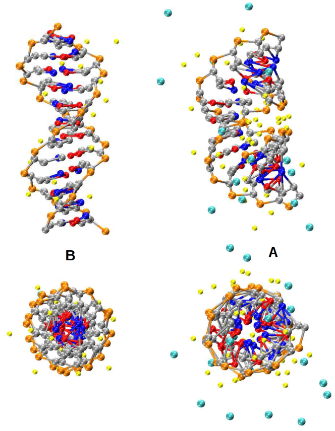
Figure 8: Frames from the trajectories A-a of sugar CG A-DNA (on the right) and B-DNA (on the left). Temperature is 300 K. Sodium ions are yellow, chlorine - cyan.

We compared the behavior of the A- and B-DNA in our sugar CG model and in the all atom AMBER force field in Appendix C in Supplemental Material Sup . Tables S11 and S12 list the lengths and the angles. As one should expect, our model proved to be stiffer than the all atom one (we accepted the maximal rigidities observed in all atom simulations), and the angles in both the A- and B-DNA are closer to their values in the all-atom A-DNA (so we set them). The only exception is dihedral angle $\angle$C3’C1’NC, for which the prescribed magnitude was (-32⁰), while the observed one - (-50⁰) in the A-DNA and (-40⁰) in the B-DNA. Interestingly, that the value for the A-DNA is in excellent agreement with the crystallographic value (GLACTONE ”ideal” DNA structures constructed by GLACTONE program according to averaged X-ray data, see G.R. Parslow, E.J. Wood (1998)): see table S4 . As regards the ribose flexibility, the CG model imitates the all-atom A-DNA very closely, including sequence dependence (see fig. S5 ). The sugar CG B-DNA is stiffer than the all atom one, and has lower population in the area between C2’-endo and C3’-endo (fig. S6 ).

When we put the A-DNA into the large reservoir, we saw the A to B phase transition within 2 nanoseconds A-a . The B-DNA transformed into A-DNA in the small reservoir during 6 nanoseconds (after waiting for 14 ns). We plan to study both the transitions more closely in the next work.

IV.3 A-DNA and ion-DNA interactions

A-DNA can exist only if sodium ions can assemble in the major groove so that their electrostatic interaction with the phosphate beads (and with the nearest chlorine ions) will give the gain in free energy greater than the loss in entropic contribution because of the ion clustering (see the balance of interactions in CG DNA forms in fig. S7 ). For the stabilization of this positively charged cluster between two rows of negative charges, the presence of a solvent in the major groove is crucial.

To adequately model this balance, we very precisely chose the positions and the widths of the minima of the effective solvent-mediated potentials. We built our potentials for the Na⁺-P and Na⁺-Na⁺ pairs so that the CG radial distribution functions g(r) were as close as possible to the all atom ones, especially in what regards the positions of the minima. The agreement between the CG rdf and the all atom one for the pair Na⁺-P in the A-DNA is almost ideal (see fig. S8 ). For the pair Na⁺-Na⁺ it was impossible because we simulated A-DNA in water, and not in mixed ethanol/water solution. A-DNA with counterions in water does not exist without additional salt. Therefore we had many more sodium ions in the computational cell, and, correspondingly, in the major groove. It had to lead to the substantial rise of the first peak as compared with the second one (see fig. S10 ), which usually takes place with increase of the salt concentration Shen et al. (2011). However, our Na⁺-P and Na⁺-Na⁺ pairs are more sticky than for the default AMBER ions (Aqvist’s cations Ȧqvist (1990)). One can see that from rdfs for B-DNA shown in fig. S9 and S11 .

Because of the evident problems of choice of ion parameters in the framework of additive, nonpolarizable and pairwise potentials, there are several different sets of ion parameters in the all atom force fields. Aqvist’s cations and Dang’s Cl^-, which were used in AMBER by default, give the artefact of formation of stable ion pairs and even salt crystals at moderately low concentrations (below their solubility limit). Other sets of the parameters result in rdfs greatly differing in shape Noy et al. (2009). To provide the agreement of the pressure inside the DNA arrays with experiment, one has to introduce additional corrections to the ion parameters Yoo and Aksimentiev (2012).

As compared with the default AMBER ions, our CG model gives for the pair Na⁺-P a very high first peak (see fig. S9 ), which means that our Na⁺ ions are more often located near phosphates, and, consequently, one to another (see fig. S11 ). The rdf for the Na⁺-P pair for B-DNA in our model mostly resembles the corresponding rdf for Cheatham’s ions Joung and Cheatham III (2008). When compared to the others, Cheatham’s sodium ions are much more often near phospates, avoiding chlorine ions and each other Noy et al. (2009). This feature seems to be a drawback leading to over-neutralization of the DNA. However, it proved to be Giambaşu et al. (2015) that the number of Cheatham’s sodium ions well agrees with ion counting experiments at low salt concentrations, and at high concentrations ($>$0.7M) is even less than in experiment. Therefore, we can regard our effective potentials for ion interactions as trustworthy.

V Discussion

We built our CG representation of the ribose flexibility on the basis of the all atom force field AMBER (Parm99SB+bsc0 Wang et al. (2000); Hornak et al. (2006); Perez et al. (2007)). Starting from it, we faced the problem that our CG DNA can assume a B-form structure at almost every reasonable set of parameters, while balancing interactions in the A-DNA required some efforts.

First, we supposed that an A-DNA can exist without placing partial charges on the bases, i.e. without introduction of sequence dependence. But that proved to be impossible. At temperature only as high as 300 K, the conglomerate of A-DNA proved to be unstable, the charges on the borders of the major groove were insufficient to keep the ions inside this groove.

Secondly, the potentials and the constants, derived from the AMBER force field, required corrections. Namely, for all the CG bonds and the CG angles (except for C1’P and P(1)P(2) connected with ribose flexibility) we used equilibrium values of the all-atom A-DNA and maximal rigidities observed in the all-atom simulations. For the double-well potential of the CG bond C1’P we lower the A-minimum to the level of the B-minimum (see fig. S2 Sup ). In this connection, one can remember that to provide a spontaneous B to A transition of d[CCAACGTTGG]₂ sequence in 85% ethanol solution in the framework of the AMBER force field, the authors had to make ”reduction of the V2 term in the O-C-C-O torsions from 1.0 to 0.30 kcal/mol to better stabilize the C3’-endo sugar pucker” Cheatham III et al. (1997).

Finally, we had to exploit such effective potentials between sodium ions and phosphate beads and between sodium ions one with another that resulted in a rdf for the pair Na⁺-P very close to the rdf for Cheatham’s ions (see fig. S9 ), and not to the rdf for default AMBER ions (for more details, see section IV.3). Evidently, the necessity of these corrections is a result of the long known ”B-philia” of the AMBER force field Feig and Pettitt (1997). Indeed, the B to A transition at high salt concentration has been demonstrated Yang and Pettitt (1996) for the ”A-philic” CHARMM force field in 1996, while for the AMBER force field this transition takes place only in a tiny drop of water Mazur (2003). In it, the compact A-DNA is stabilized by surface tension. The additional salt results only in salt crystallization, instead of the B to A transition.

After the described fitting, we have obtained both an A-DNA and a B-DNA at the corresponding conditions, as well as both A$\rightarrow$B and B$\rightarrow$A transitions.

VI Conclusions

We saw that the offered CG representation of the ribose flexibility in the sugar CG DNA model is adequate, as it provides the geometric possibility of existence of both the A- and B-forms of dsDNA. The proposed scheme is obtained by physically clear ”bottom-up” approach and therefore should work equally well in both ss- and dsDNA. This scheme seems to be the last needed component to adequately represent the deformability of a CG DNA strand, and, consequently, the CG dsDNA molecule.

We have shown that to obtain the correct balance of interactions in A- and in B-DNA at the corresponding conditions (high and low salt concentrations), one should explicitly introduce charges on the nucleotides and salt ions. Besides the charges on the phosphates, one should place the partial charges on the beads of the bases.

As is easy to see, our method of ”relaxation” which we used to derive the double-well potential describing ribose flexibility is a variant of the ”derived coarse graining” Brini et al. (2013), only, for the interaction between the beads, we adopted the minimum energy of all possible all-atom configurations, instead of the mean value. This is justified because, contrary to the case of liquids, the configurations with high energies are highly improbable on the CG time scale. The rigidities of the CG bonds and angles, although obtained by the Boltzmann inversion method (belonging to the ”parameterized coarse graining” which results are normally state-point dependent), should not have noticeable temperature dependence, because we used relatively ”fine” mapping (each bead corresponds to a relatively small number of atoms) Foley et al. (2015). The electrostatic DNA-ion and ion-ion interactions contribute much more than the bonded interactions to the entropic component of the many-body potential of mean force. These potentials include solvation effects and are highly temperature-dependent (we adopted the parametrization for T=300 K).

The proposed CG realization of the ribose flexibility is computationally cheap. Together with CG interactions between bases, the sugar CG DNA model allows to promptly check physical hypotheses in extensive simulations of long DNA molecules. First of all, the sugar CG model can be applied for modeling of large mechanical deformations of long DNA molecules, and not only for simulation of in vitro experiments. The charges on the bases (depending on the base type) allows one to use the model for studying DNA-protein interactions, including the interactions with CG proteins. A small change of the model enables base openings, and offers the possibility to simulate DNA denaturation, and to investigate transcription and replication. As the model includes explicit ions, one can model electrostatic interactions of DNA and DNA-protein complexes with different types of ions in different solvents. So, for the present, the model seems to be universal: it includes all the needed features to be employed for any application in biophysics and nanotechnology.