Origin and Loss of nebula-captured hydrogen envelopes
from ‘sub’- to ‘super-Earths’ in the habitable zone
of Sun-like stars

Abstract

We investigate the origin and loss of captured hydrogen envelopes from protoplanets having masses in a range between ‘sub-Earth’-like bodies of 0.1$M_{\oplus}$ and ‘super-Earths’ with 5$M_{\oplus}$ in the habitable zone at 1 AU of a Sun like G star, assuming that their rocky cores had formed before the nebula gas dissipated. We model the gravitational attraction and accumulation of nebula gas around a planet’s core as a function of protoplanetary luminosity during accretion and calculate the resulting surface temperature by solving the hydrostatic structure equations for the protoplanetary nebula. Depending on nebular properties, such as the dust grain depletion factor, planetesimal accretion rates, and resulting luminosities, for planetary bodies of 0.1–1$M_{\oplus}$ we obtain hydrogen envelopes with masses between $\sim 2.5\times 10^{19}$–$1.5\times 10^{26}$ g. For ‘super-Earths’ with masses between 2–5$M_{\oplus}$ more massive hydrogen envelopes within the mass range of $\sim 7.5\times 10^{23}$–$1.5\times 10^{28}$ g can be captured from the nebula. For studying the escape of these accumulated hydrogen-dominated protoatmospheres, we apply a hydrodynamic upper atmosphere model and calculate the loss rates due to the heating by the high soft-X-ray and extreme ultraviolet (XUV) flux of the young Sun/star. The results of our study indicate that under most nebula conditions ‘sub-Earth’ and Earth-mass planets can lose their captured hydrogen envelopes by thermal escape during the first $\sim 100$ Myr after the disk dissipated. However, if a nebula has a low dust depletion factor or low accretion rates resulting in low protoplanetary luminosities, it is possible that even protoplanets with Earth-mass cores may keep their hydrogen envelopes during their whole lifetime. In contrast to lower mass protoplanets, more massive ‘super-Earths’ that can accumulate a huge amount of nebula gas, lose only tiny fractions of their primordial hydrogen envelopes. Our results agree with the fact that Venus, Earth, and Mars are not surrounded by dense hydrogen envelopes, as well as with the recent discoveries of low density ‘super-Earths’ that most likely could not get rid of their dense protoatmospheres.

1 INTRODUCTION

During the growth from planetesimals to planetary embryos and the formation of protoplanets in the primordial solar nebula, massive hydrogen/helium envelopes can be captured (e.g., Mizuno et al. 1978; Wuchterl 1993; Ikoma et al. 2000; Rafikov 2006). The capture of nebula gas becomes important when the growing planetary embryos grow to a stage, where gas accretion exceeds solid body accretion, so that the massive gaseous envelopes of Jupiter-type planets can be formed (e.g., Pollack 1985; Lissauer et al. 1995; Wuchterl 1995; 2010).

Analytical and numerical calculations indicate that the onset of core instability occurs when the mass of the hydrogen atmosphere around the core becomes comparable to the core mass (e.g., Hayashi et al. 1978; Mizuno et al. 1978; Mizuno 1980; Stevenson 1982; Wuchterl 1993; 1995; Ikoma et al. 2000; Rafikov 2006; Wuchterl 2010). This fast growth of nebula-based hydrogen envelopes occurs if the core reaches a mass of $\sim 10M_{\rm\oplus}$ and a size of $\sim 2R_{\rm\oplus}$ (e.g., Alibert et al. 2010).

As it was shown in the early pioneering studies by Mizuno et al. (1978; 1980) and Hayashi et al. (1979) if the core mass becomes $\geq 0.1M_{\rm\oplus}$, depending on nebula properties, an appreciable amount of the surrounding nebula gas can be captured by terrestrial-type protoplanets such as proto-Venus or proto-Earth to form an optically thick, dense primordial hydrogen atmosphere with a mass in the order of $\sim 10^{26}$g or $\sim 653$ Earth ocean equivalent amount of hydrogen (EO_H). Because Earth doesn’t have such a hydrogen envelope at present, Sekiya et al. (1980a; 1980b) studied the evaporation of this primordial nebula-captured terrestrial atmosphere due to irradiation of the solar EUV radiation of the young Sun.

These authors suggested that Earth’s nebula captured hydrogen envelope of the order of $\sim 10^{26}$ g should have dissipated within a period of $\sim 500$ Myr, because $\sim$4 Gyr ago nitrogen was the dominant species in the atmosphere. It was found that for removing the expected hydrogen envelope during the time period of $\sim 500$ Myr, the EUV flux of the young Sun should have been $\sim 200$ times higher compared to the present day value. However, Sekiya et al. (1980a; 1980b) concluded that such a high EUV flux during this long time period was not realistic. To overcome this problem, Sekiya et al. (1981) assumed in a follow up study a far-UV flux, that was $\sim 100$ times higher compared to that of the present Sun during the T-Tauri stage and its absorption occurred through photodissociation of H₂O molecules. Under this assumptions Earth’s, protoatmosphere dissipated within $\sim 20$ Myr (Sekiya et al. 1981).

However, the results and conclusions of these pioneering studies are based on very rough assumptions, because decades ago, no good observational data from disks and related nebula lifetimes, as well as astrophysical observations of the radiation environment of very young solar-like stars have been available. Since that time several multiwavelength satellite observations of the radiation environment of young solar-like stars indicate that the assumed EUV and far-UV flux values by Sekiya et al. (1980b; 1981) have been too high and/or lasted for shorter timescales (Guinan et al. 2003; Ribas et al. 2005; Güdel 2007; Claire et al. 2012; Lammer et al. 2012; and references therein).

The main aim of this study is to investigate the capture and loss of nebula-based hydrogen envelopes from protoplanets with ‘sub-‘to ‘super-Earth’ masses, during the XUV saturated phase of a Sun-like star (e.g., Ayres 1997; Güdel et al. 1995; Güdel 1997; Güdel et al. 1997; Guinan et al. 2003; Ribas et al. 2005; Claire et al. 2012), in the habitable zone (HZ) at 1 AU. In Sect. 2 we discuss the latest stage of our knowledge regarding the early solar/stellar radiation environment from the time when the nebula dissipated and protoplanetary atmospheres have been exposed freely to the high solar XUV radiation field. In Sect. 3 we study the formation of nebula captured hydrogen envelopes on protoplanets with an Earth-like mean core density and core masses of 0.1$M_{\rm\oplus}$, 0.5$M_{\rm\oplus}$, 1$M_{\rm\oplus}$, 2$M_{\rm\oplus}$, 3$M_{\rm\oplus}$, and 5$M_{\rm\oplus}$ by solving the hydrostatic structure equations for the protoplanetary nebula for different dust grain depletion factors, planetesimal accretion rates, and corresponding protoplanetary luminosities. In Sect. 4 we study the heating and expansion of the captured hydrogen envelopes by the XUV radiation, as well as the related thermal escape rates during the XUV saturation phase of the young Sun/stars by applying a time-dependent numerical algorithm, that solves the system of 1-D fluid equations for mass, momentum, and energy conservation. Finally we discuss our results and their implications for the formation of early Venus, Earth, Mars, terrestrial exoplanets, and habitability in general.

2 THE EARLY XUV ENVIRONMENT OF SOLAR-LIKE STARS

2.1 The XUV activity during the stellar saturation phase

The evolution of the solar high-energy radiation has been studied in detail within the ‘Sun in Time’ program (e.g., Ribas et al. 2005; Güdel 2007). At ages higher than about 0.1 Gyr, the activity of Sun-like stars decreases because of magnetic braking by the stellar wind. Data from X-rays to UV from a sample of solar analogs of different ages provided power laws of the solar fluxes in different wavelength bands within the XUV range (1–1200 Å) as a function of age. Recently, Claire et al. (2012) extended this study to longer wavelengths and provided a code with calculates full spectra from X-rays to the infrared for a range of stellar ages. Using their model, we calculate solar fluxes in several wavelength bands back to an age of 0.1 Gyr, which corresponds approximately to the end of the saturation period for a Sun-like star (Fig. 1). We normalize the derived XUV fluxes to the present-day (4.56 Gyr) value of $5.27\,\mathrm{erg\,cm^{-2}\,s^{-1}}$ as calculated with the model of Claire et al. (2012), which corresponds to the Sun’s emission during activity maximum, to obtain the evolution of the flux enhancement factor. This fiducial value is slightly higher than the moderate solar value of $4.64\,\mathrm{erg\,cm^{-2}\,s^{-1}}$ adopted by Ribas et al. (2005), but the evolution of the flux enhancement factor calculated with their power law is almost identical. We prefer the spectral model mainly because we are interested in the evolution of other wavelength bands for which no power laws were given by Ribas et al. (2005). Note that the XUV flux of the present-day Sun is highly variable and may change by up to an order of magnitude. In this section we adopt the fiducial values derived from the Claire et al. (2012) model for 4.56 Gyr to simply set the Sun at one in Fig. 1.

During the saturation phase of a solar-like G-type star ($\leq 0.1$ Gyr), the stellar X-ray luminosity is saturated at a level of about 0.1% of the bolometric luminosity (Pizzolato et al. 2003; Jackson et al. 2012). Before the Sun reached the main sequence, its bolometric luminosity varied strongly according to stellar evolution models. Hence, the high-energy emission is expected to roughly follow the evolution of the bolometric luminosity. This is consistent with X-ray observations of solar-type stars in young clusters. To estimate the Sun’s XUV emission during the saturation phase, we use an evolution model from Baraffe et al. (1998) for a solar-mass star and adopt an X-ray saturation level of $L_{\mathrm{X,sat}}=10^{(-3.2\pm 0.3)}L_{\mathrm{bol}}$ from Pizzolato et al. (2003) for stars of about one solar mass. We assume that most of the XUV emission during this phase is emitted in X-rays, however, the unknown contribution at longer wavelengths may increase the scaling factor. We caution that the estimated enhancement factor during this period is very uncertain. However, in agreement with the normalized values shown in Fig. 1 we apply for the thermal escape model below, an average XUV enhancement factor during the saturation phase of the solar-like star that is 100 times higher compared to the value at 1 AU of today’s Sun.

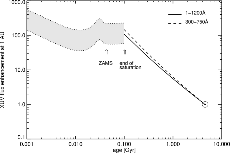
Figure 1: Evolution of the solar high-energy emission in different wavelength bands calculated with the model of Claire et al. (2012). All fluxes are taken at 1 AU and normalized to the present solar values of $[5.27,1.69]\,\mathrm{erg\,cm^{-2}\,s^{-1}}$ for the XUV, EUV bands. Before 0.1 Gyr the Sun’s XUV evolution is approximated by the modeled evolution of the bolometric luminosity of a star of $1M_{\odot}$ (Baraffe et al. 1998) and an X-ray saturation level of $10^{-3.2\pm 0.3}L_{\mathrm{bol}}$ (Pizzolato et al. 2003), denoted by the shaded area. Arrows indicate the zero-age main sequence (ZAMS) and the approximate end of the saturation phase.

2.2 The dissipation time of the nebula gas

The capture of primordial atmospheres by accreting protoplanetary cores depend mainly on the nebula lifetime, nebula parameters such as the dust-depletion factor, core mass, and core accretion luminosity. The life time of the nebula can be estimated from infrared observations of T-Tauri stars in star forming regions, that are sensitive to the presence of circumstellar material. Such observations indicate that disks evaporate and disappear on different timescales (e.g., Hillenbrand 2006; Montmerle et al. 2006). Inner disks where the regions are warm enough to radiate at near-IR wavelengths disappear after a few Myrs (Hillenbrand 2006). The fraction of stars with discs is consistent with 100% at an age of 1 Myr, and drops to less than 10% after 10 Myr. There are some observations of older disks but their masses are too low to form a Jupiter-like gas giant. Therefore, the common view is that giant planets must form on timescales which are $<10$ Myr (Montmerle et al. 2006; and references therein). Because of this fact, one can expect that cores with masses from ‘sub’- to ‘super-Earths’ can also be formed during the time before the nebula gas evaporates.

3 ORIGIN OF NEBULA-CAPTURED PROTOATMOSPHERES

Table 1: Masses and surface properties of captured protoatmospheres around rocky cores of 0.1$M_{\rm\oplus}$, 0.5$M_{\rm\oplus}$, 1$M_{\rm\oplus}$, 2$M_{\rm\oplus}$, 3$M_{\rm\oplus}$, and 5$M_{\rm\oplus}$ using a dust depletion factor $f$ of 0.001. The relative accretion rate $\dot{M}_{\rm acc}/M_{\rm pl}$ is a free parameter and defines a planetary luminosity $L_{\rm pl}$. $T_{\rm s}$ and $P_{\rm s}$ are the surface temperature and pressure, the atmospheric mass $M_{\rm atm}$ is given in g and Earth ocean equivalent amounts of hydrogen EO_H. The hydrogen envelope mass fraction is defined as $f_{\rm env}=M_{\rm atm}/M_{\rm pl}$, where $M_{\rm pl}=(M_{\rm atm}+M_{\rm core})$.

$M_{\rm core}$ [$M_{\rm\oplus}$]	$R_{\rm pl}$ [$R_{\rm\oplus}$]	$\frac{\dot{M}_{\rm acc}}{M_{\rm pl}}$ [yr-1]	$L_{\rm pl}$ [erg s-1]	$T_{\rm s}$ [K]	$P_{\rm s}$ [bar]	$M_{\rm atm}$ [g]	$M_{\rm atm}$ [EOH]	$f_{\rm env}$
0.1	0.46	$10^{-5}$	$2.54\times 10^{25}$	961	0.155	$2.13\times 10^{21}$	0.014	$3.6\times 10^{-6}$
0.5	0.79	$10^{-5}$	$3.71\times 10^{26}$	2687	4.703	$2.19\times 10^{23}$	1.429	$7.3\times 10^{-5}$
1	1	$10^{-5}$	$1.18\times 10^{27}$	3594	24.81	$1.47\times 10^{24}$	9.608	$2.5\times 10^{-4}$
2	1.26	$10^{-5}$	$3.74\times 10^{27}$	4780	168.8	$1.01\times 10^{25}$	66.01	$8.4\times 10^{-4}$
3	1.44	$10^{-5}$	$7.35\times 10^{27}$	5810	558.2	$3.24\times 10^{25}$	211.5	$1.8\times 10^{-3}$
5	1.71	$10^{-5}$	$1.72\times 10^{28}$	7792	2503	$1.46\times 10^{26}$	956.2	$4.9\times 10^{-3}$
0.1	0.46	$10^{-6}$	$2.54\times 10^{24}$	871	0.768	$7.18\times 10^{21}$	0.047	$1.2\times 10^{-5}$
0.5	0.79	$10^{-6}$	$3.71\times 10^{25}$	2749	26.73	$9.60\times 10^{23}$	6.275	$3.2\times 10^{-4}$
1	1	$10^{-6}$	$1.18\times 10^{26}$	3802	134.7	$6.82\times 10^{24}$	44.6	$1.1\times 10^{-3}$
2	1.26	$10^{-6}$	$3.74\times 10^{26}$	5224	833.8	$4.88\times 10^{25}$	319	$4.1\times 10^{-3}$
3	1.44	$10^{-6}$	$7.35\times 10^{26}$	6423	2561	$1.58\times 10^{26}$	1030	$8.7\times 10^{-3}$
5	1.71	$10^{-6}$	$1.72\times 10^{27}$	8690	10377	$7.12\times 10^{26}$	4653	0.023
0.1	0.46	$10^{-7}$	$2.54\times 10^{23}$	770	3.329	$2.29\times 10^{22}$	0.15	$3.8\times 10^{-5}$
0.5	0.79	$10^{-7}$	$3.71\times 10^{24}$	2729	154.4	$4.32\times 10^{24}$	28.2	$1.4\times 10^{-3}$
1	1	$10^{-7}$	$1.18\times 10^{25}$	3972	744.6	$3.21\times 10^{25}$	210	$5.4\times 10^{-3}$
2	1.26	$10^{-7}$	$3.74\times 10^{25}$	5601	4126	$2.40\times 10^{26}$	1565	0.020
3	1.44	$10^{-7}$	$7.35\times 10^{25}$	6955	11742	$8.06\times 10^{26}$	5270	0.043
5	1.71	$10^{-7}$	$1.72\times 10^{26}$	9494	45193	$4.38\times 10^{27}$	28620	0.13
0.1	0.46	$10^{-8}$	$2.55\times 10^{22}$	677	10.70	$5.99\times 10^{22}$	0.392	$1.0\times 10^{-4}$
0.5	0.79	$10^{-8}$	$3.72\times 10^{23}$	2648	772.9	$1.79\times 10^{25}$	116.7	$5.9\times 10^{-3}$
1	1	$10^{-8}$	$1.18\times 10^{24}$	3987	3929	$1.53\times 10^{26}$	1002	0.025
2	1.26	$10^{-8}$	$3.74\times 10^{24}$	5722	21892	$1.52\times 10^{27}$	9934	0.11
3	1.44	$1.41\times 10^{-8}\,{}^{a}$	$1.04\times 10^{25}$	7291	63099	$8.67\times 10^{27}$	56640	0.33
5	1.71	$5.11\times 10^{-8}\,{}^{a}$	$8.81\times 10^{25}$	9955	96262	$1.62\times 10^{28}$	105816	0.35

${}^{a})$ Accretion rate increased to obtain a stationary solution.

Table 2: Same as Tab. 1 for a dust depletion factor $f$ of 0.01

.

$M_{\rm core}$ [$M_{\rm\oplus}$]	$R_{\rm pl}$ [$R_{\rm\oplus}$]	$\frac{\dot{M}_{\rm acc}}{M_{\rm pl}}$ [yr-1]	$L_{\rm pl}$ [erg s-1]	$T_{\rm s}$ [K]	$P_{\rm s}$ [bar]	$M_{\rm atm}$ [g]	$M_{\rm atm}$ [EOH]	$f_{\rm env}$
0.1	0.46	$10^{-5}$	$2.54\times 10^{25}$	924	0.033	$3.41\times 10^{20}$	0.0022	$5.7\times 10^{-7}$
0.5	0.79	$10^{-5}$	$3.71\times 10^{26}$	2412	1.299	$3.47\times 10^{22}$	0.227	$1.2\times 10^{-5}$
1	1	$10^{-5}$	$1.18\times 10^{27}$	3307	8.395	$2.57\times 10^{23}$	1.682	$4.3\times 10^{-5}$
2	1.26	$10^{-5}$	$3.74\times 10^{27}$	4436	68.93	$2.12\times 10^{24}$	13.84	$1.8\times 10^{-4}$
3	1.44	$10^{-5}$	$7.35\times 10^{27}$	5399	254.0	$8.09\times 10^{24}$	52.86	$4.5\times 10^{-4}$
5	1.71	$10^{-5}$	$1.72\times 10^{28}$	7210	1288	$4.57\times 10^{25}$	299	$1.5\times 10^{-3}$
0.1	0.46	$10^{-6}$	$2.54\times 10^{24}$	848	0.184	$2.26\times 10^{21}$	0.014	$3.8\times 10^{-6}$
0.5	0.79	$10^{-6}$	$3.71\times 10^{25}$	2516	8.122	$2.72\times 10^{23}$	1.776	$9.1\times 10^{-5}$
1	1	$10^{-6}$	$1.18\times 10^{26}$	3563	46.92	$1.96\times 10^{24}$	12.8	$3.3\times 10^{-4}$
2	1.26	$10^{-6}$	$3.74\times 10^{26}$	4865	334.1	$1.47\times 10^{25}$	96.14	$1.2\times 10^{-3}$
3	1.44	$10^{-6}$	$7.35\times 10^{26}$	5979	1120	$4.99\times 10^{25}$	326.2	$2.8\times 10^{-3}$
5	1.71	$10^{-6}$	$1.72\times 10^{27}$	8091	5040	$2.45\times 10^{26}$	1600	$8.1\times 10^{-3}$
0.1	0.46	$10^{-7}$	$2.54\times 10^{23}$	790	0.956	$8.06\times 10^{21}$	0.052	$1.3\times 10^{-5}$
0.5	0.79	$10^{-7}$	$3.71\times 10^{24}$	2590	49.28	$1.33\times 10^{24}$	8.673	$4.4\times 10^{-4}$
1	1	$10^{-7}$	$1.18\times 10^{25}$	3772	264.3	$1.01\times 10^{25}$	65.75	$1.7\times 10^{-3}$
2	1.26	$10^{-7}$	$3.74\times 10^{25}$	5304	1644	$7.66\times 10^{25}$	500.3	$6.4\times 10^{-3}$
3	1.44	$10^{-7}$	$7.35\times 10^{25}$	6577	4997	$2.57\times 10^{26}$	1680	0.014
5	1.71	$10^{-7}$	$1.72\times 10^{26}$	8956	19911	$1.24\times 10^{27}$	8117	0.040
0.1	0.46	$10^{-8}$	$2.55\times 10^{22}$	717	4.441	$2.80\times 10^{22}$	0.183	$4.7\times 10^{-5}$
0.5	0.79	$10^{-8}$	$3.72\times 10^{23}$	2623	276.9	$6.42\times 10^{24}$	41.95	$2.1\times 10^{-3}$
1	1	$10^{-8}$	$1.18\times 10^{24}$	3933	1408	$5.09\times 10^{25}$	332.6	$8.4\times 10^{-3}$
2	1.26	$10^{-8}$	$3.74\times 10^{24}$	5626	7910	$4.09\times 10^{26}$	2670	0.033
3	1.44	$10^{-8}$	$7.35\times 10^{24}$	7013	22656	$1.50\times 10^{27}$	9797	0.077
5	1.71	$1.11\times 10^{-8}\,{}^{a}$	$1.91\times 10^{25}$	9894	105653	$1.59\times 10^{28}$	103725	0.35

${}^{a})$ Accretion rate increased to obtain a stationary solution.

Table 3: Same as Tab. 1 for a dust depletion factor $f$ of 0.1.

$M_{\rm core}$ [$M_{\rm\oplus}$]	$R_{\rm pl}$ [$R_{\rm\oplus}$]	$\frac{\dot{M}_{\rm acc}}{M_{\rm pl}}$ [yr-1]	$L_{\rm pl}$ [erg s-1]	$T_{\rm s}$ [K]	$P_{\rm s}$ [bar]	$M_{\rm atm}$ [g]	$M_{\rm atm}$ [EOH]	$f_{\rm env}$
0.1	0.46	$10^{-5}$	$2.54\times 10^{25}$	1031	0.006	$2.65\times 10^{19}$	0.00017	$4.4\times 10^{-8}$
0.5	0.79	$10^{-5}$	$3.71\times 10^{26}$	1810	0.291	$4.48\times 10^{21}$	0.029	$1.5\times 10^{-6}$
1	1	$10^{-5}$	$1.18\times 10^{27}$	2956	3.287	$4.84\times 10^{22}$	0.316	$8.1\times 10^{-6}$
2	1.26	$10^{-5}$	$3.74\times 10^{27}$	4131	37.43	$7.26\times 10^{23}$	4.747	$6.1\times 10^{-5}$
3	1.44	$10^{-5}$	$7.35\times 10^{27}$	5081	160.5	$3.58\times 10^{24}$	23.37	$2.0\times 10^{-4}$
5	1.71	$10^{-5}$	$1.72\times 10^{28}$	6872	946.9	$2.60\times 10^{25}$	169.6	$8.7\times 10^{-4}$
0.1	0.46	$10^{-6}$	$2.54\times 10^{24}$	901	0.034	$3.53\times 10^{20}$	0.0023	$5.9\times 10^{-7}$
0.5	0.79	$10^{-6}$	$3.71\times 10^{25}$	1885	1.723	$3.77\times 10^{22}$	0.0246	$1.3\times 10^{-5}$
1	1	$10^{-6}$	$1.18\times 10^{26}$	3092	16.79	$3.54\times 10^{23}$	2.313	$5.9\times 10^{-5}$
2	1.26	$10^{-6}$	$3.74\times 10^{26}$	4440	165.4	$3.82\times 10^{24}$	24.95	$3.2\times 10^{-4}$
3	1.44	$10^{-6}$	$7.35\times 10^{26}$	5524	645.8	$1.65\times 10^{25}$	107.8	$9.2\times 10^{-4}$
5	1.71	$10^{-6}$	$1.72\times 10^{27}$	7566	3427	$1.06\times 10^{26}$	690.8	$3.5\times 10^{-3}$
0.1	0.46	$10^{-7}$	$2.54\times 10^{23}$	803	0.192	$2.29\times 10^{21}$	0.014	$3.8\times 10^{-6}$
0.5	0.79	$10^{-7}$	$3.71\times 10^{24}$	2001	11.36	$3.02\times 10^{23}$	1.971	$1.0\times 10^{-4}$
1	1	$10^{-7}$	$1.18\times 10^{25}$	3302	94.54	$2.57\times 10^{24}$	16.8	$4.3\times 10^{-4}$
2	1.26	$10^{-7}$	$3.74\times 10^{25}$	4832	782.6	$2.35\times 10^{25}$	153.2	$2.0\times 10^{-3}$
3	1.44	$10^{-7}$	$7.35\times 10^{25}$	6071	2737	$8.94\times 10^{25}$	584.1	$5.0\times 10^{-3}$
5	1.71	$10^{-7}$	$1.72\times 10^{26}$	8341	12608	$4.97\times 10^{26}$	3250	0.016
0.1	0.46	$10^{-8}$	$2.55\times 10^{22}$	728	1.032	$8.34\times 10^{21}$	0.054	$1.4\times 10^{-5}$
0.5	0.79	$10^{-8}$	$3.72\times 10^{23}$	2180	76.42	$1.65\times 10^{24}$	10.75	$5.5\times 10^{-4}$
1	1	$10^{-8}$	$1.18\times 10^{24}$	3537	528.3	$1.43\times 10^{25}$	93.2	$2.4\times 10^{-3}$
2	1.26	$10^{-8}$	$3.74\times 10^{24}$	5212	3736	$1.26\times 10^{26}$	826.1	0.010
3	1.44	$10^{-8}$	$7.35\times 10^{24}$	6542	11790	$4.69\times 10^{26}$	3066	0.026
5	1.71	$10^{-8}$	$1.72\times 10^{25}$	8974	48871	$2.73\times 10^{27}$	17810	0.084

Once protoplanets orbiting a host star embedded in a protoplanetary nebula gain enough mass for their gravitational potential to become significant relatively to the local gas internal and turbulent motion energy, they will start to accumulate nebula gas into their atmospheres. Hydrostatic and spherically symmetric models of such primary hydrogen atmospheres have been applied by Hayashi et al. (1979) and Nakazawa et al. (1985) assuming a continuous influx of planetesimals which generated planetary luminosity. The planetesimals are assumed to travel through the atmosphere without energy losses so that the gained gravitational energy has been released on the planetary surface. More recently, Ikoma and Genda (2006) improved these earlier results by adopting a more realistic equation of state and opacities, as well as an extended parameter space. In particular, this is the first study which uses detailed dust opacity data, i.e. includes evaporation/condensation of various dust species which directly affects the atmospheric structure.

To estimate the amount of nebula gas collected by a protoplanet from the surrounding protoplanetary disk, we considered a series of solid (rocky) cores with masses of 0.1, 0.5, 1, 2, 3, and 5 $M_{\rm\oplus}$ and an average core density $\rho_{\rm core}$ of 5.5 g cm^-3 and computed self-gravitating, hydrostatic, spherically symmetric atmospheres around those bodies. Spherical symmetry is a good assumption in the inner parts of the planetary atmosphere, but less so in the outer part, where the atmospheric structure melds into the circumstellar disk. Therefore we fixed the outer boundary of our models at the point where the gravitational domination of the planet will finally break down, i.e. the Hill radius defined as

$$R_{\rm H}=\left(\frac{M_{\rm pl}}{3M_{\star}}\right)^{1/3}d\;,$$ (1)

where $d$ is the semi-major axis of the planetary orbit. Because we are interested in studying the capture and losses of hydrogen envelopes within the HZ of a Sun-like star, we assume $d$=1 AU and $M_{\star}=M_{\odot}$ for all model runs. When evaluating the captured atmospheric mass, we included only the atmospheric structure up to the Bondi radius

$$R_{\rm B}=\frac{G\;M_{\rm pl}}{h}\;.$$ (2)

(which usually is about an order of magnitude smaller than $R_{\rm H}$). Beyond $R_{\rm B}$ the enthalpy $h$ of the gas exceeds the gravitational potential, thus the gas is not effectively bound to the planet and will escape once the nebula disappears.

For the physical conditions in the circumstellar disk (i.e. at $R_{\rm H}$), in particular temperature and density, we assume T = 200 K and $\rho=5\times 10^{-10}$ g cm^-3, in accordance with models of the initial mass planetary nebula (Hayashi, 1981). We would like to stress the point that in our models the atmospheric masses of substantial atmospheres (with the surface pressure greater than $\sim 1$ bar) are rather insensitive to the location of the outer boundary (i.e. $M_{\star}$ and $d$) and to the physical conditions at this location. This fact is in agreement with the earlier studies of planetary atmospheres with radiative outer envelopes (e.g. Stevenson, 1982; Wuchterl, 1993; Rafikov, 2006).

The temperature of the planetary atmosphere is determined by the planetary luminosity, which in turn is connected to the continuous accretion of planetesimals onto the planet. The observed lifetimes of protoplanetary disks of some Myrs give some constrains on the formation times of the planetary cores, accordingly we adopted mass accretion rates $\dot{M}_{\rm acc}/M_{\rm pl}$ of $10^{-5}{\rm yr}^{-1}$, $10^{-6}{\rm yr}^{-1}$, and $10^{-7}{\rm yr}^{-1}$. We assume that the energy release due to accretion occurs exclusively on the planetary surface, yielding a luminosity at the bottom of the atmosphere of

$$L_{\rm pl}\simeq GM_{\rm pl}\dot{M}_{\rm acc}\left(\frac{1}{r_{\rm pl}}-\frac{1}{r_{\rm H}}\right)\;.$$ (3)

Apart from the luminosity generated by accretion, it is also reasonable to assume that the planetary core stores a fraction of the internal energy generated in the formation process (Elkins-Tanton, 2008; Hamano et al., 2013) which is a quite recent event, in any case for a planet in the nebula phase. Therefore, the cooling of the core may generate a heat flux, depending on energy transport physics in the interior, contributing to the luminosity on the planetary surface. Another contribution to the planetary luminosity comes from radiogenic heat production which is assumed to be proportional to the core mass by using the reference value of $10^{21}$ erg s^-1 $M_{\rm\oplus}^{-1}$ for the young Earth (Stacey, 1992).

In order to obtain a measure for the uncertainties involved in our modelling, we investigated a parameter space spanned by the planetary luminosity $L_{\rm pl}$ and the dust depletion factor $f$. The dust depletion factor $f$ describes the abundance of dust relative to the amount of dust that would condensate from the gas in equilibrium conditions. In a hydrostatic structure, large dust grains will decouple dynamically from the gas and may thus fall (rain) toward the surface. This effect is crudely modelled by adjusting the dust depletion factor $f$. It seems clear that in general $f$ should be $<1$, but apart from that, the magnitude of $f$ remains highly uncertain. As dust opacities dominate over gas opacities usually by many orders of magnitude, $f$ in effect scales the overall opaqueness of the atmosphere. We selected these two parameters as they have a very significant effect on the atmospheric structure, and yet are very poorly constrained both from theory and observations.

The hydrostatic structure equations were integrated by using the TAPIR-Code (short for The adaptive, implicit RHD-Code). Convective energy transport is included in TAPIR by an equation for the turbulent convective energy following concepts of Kuhfuß (1987). For the gas and dust opacity we used tables from Freedman et al. (2008), and Semenov et al. (2003), respectively; for the equation of state we adopted the results of Saumon et al. (1995). Both, for the gas opacity and the equation of state we assumed solar composition and ignored chemical inhomogeneities.

Tables 1 to 3 summarize the constitutive parameters and integral properties of the computed atmosphere models. Ignoring more subtle effects caused by dust physics, opacities and convective transport, the general trends in the results for the envelope masses can be understood from the fact that planetary atmospheres are supported from collapse by both the density gradient and the temperature gradient. The amount of thermal support of a planetary atmosphere depends, (1) on the planetary luminosity, i.e. the accretion rate, and, (2) on the dust depletion factors $f$ defining the opacity and thus the insulation properties of the envelope. For a fixed atmospheric structure, more dust increases the opaqueness of the atmosphere which thus becomes warmer. Accordingly, envelopes with large dust depletion factors $f$ are more thermally supported and less massive.

Obviously, increasing the accretion rate also leads to more thermal support and smaller atmospheric masses. Inspection of Tables 1 to 3 shows that Earth-mass rocky cores capture hydrogen envelopes between $\sim 5\times 10^{22}$ and $\sim 1.5\times 10^{24}$ g (equivalent to $\sim 0.3$–10 EO_H) for a high accretion rate of $\dot{M}_{\rm acc}/M_{\rm pl}=10^{-5}$ yr^-1, whereas a low accretion rate of $\dot{M}_{\rm acc}/M_{\rm pl}=10^{-8}$ yr^-1 leads to much more massive envelopes between $\sim 1.5\times 10^{25}$ and $\sim 1.5\times 10^{26}$ g ($\sim 100$–1000 EO_H).

The most massive hydrogen envelopes are accumulated around rocky cores within the so-called ‘super-Earth’ domain for low accretion rates and small dust depletion factors and can reach up to several $\sim 10^{3}$ to $\sim 10^{4}$ EO_H. In some cases of more massive planetary cores we also encountered the upper mass limit of stationary atmospheres, i.e. the critical core mass. For these model runs we increased the accretion rate (as indicated in the tables), and thus the luminosity, to stay just above the critical limit. Such envelopes have hydrogen masses equivalent from $\sim 5\times$10⁴ to $\sim 10^{5}$ EO_H. Any further reduction of the luminosity of these planets would push them into the instability regime, causing a collapse of an atmosphere and nebula gas and putting them onto the formation path of a gas giant planet.

Our results, as presented in Tables 1 to 3, are in reasonable agreement with those of Ikoma and Genda (2006) considering the differences in input physics, in particular, dust opacity and in the implementation of the outer boundary condition. Ikoma and Genda (2006) placed the outer boundary of their models at the Bondi radius (in fact at the minimum of $r_{\rm H}$ and $r_{\rm B}$, but this turns out to be equal to the latter in all relevant cases) and accordingly implemented the physical outer boundary conditions (nebula density and temperature) much closer to the planet than in our models. Even though, as noted above, the outer boundary conditions only moderately affect the solution, this leads to somewhat more massive atmospheres.

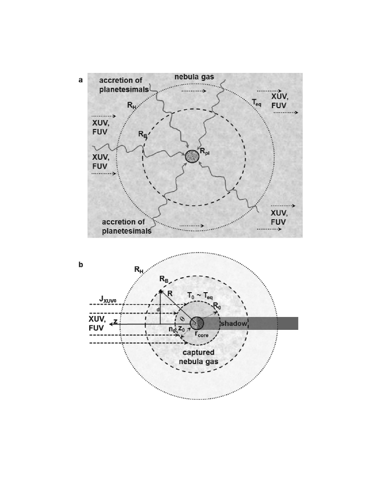
Figure 2: Illustration of the protoplanet inside the nebula gas and after its dissipation. Panel a: shaded area gas in the XUV and FUV exposed evaporating planetary disk; corrugated arrows symbolize the influx of accreting material; $T_{\rm eq}$ is the equilibrium temperature of the nebula in the planet’s orbital location; $R_{\rm H}$, $R_{\rm B}$, and $R_{\rm pl}$ correspond to the Hill radius, the Bondi radius and the planetary core radius, respectively. Panel b: illustrates the contracted protoatmosphere after the nebula is dissipated and the influx of planetesimals decreased, with radius $R_{0}$, number density $n_{0}$, and temperature $T_{0}$ that resembles the equilibrium temperature $T_{\rm eq}$ at the mesopause or the base of the thermosphere.

Finally, one should also note that the protoatmosphere models described in this section rely on the assumption that the planetary envelopes are in a stationary condition, so that the dynamical and thermal time scale of the envelope are sufficiently separated both from the cooling time scale of the solid core and the evolution time scale of the protoplanetary disk. This assumption is not necessarily fulfilled in real planetary atmospheres. To improve on the stationary models, further numerical development are planed in the future might allow for the time-dependent, dynamic simulation of such protoatmospheres (Stökl et al. 2014) and their interaction with the solid core and the disk-nebula environment.

4 XUV HEATING AND ESCAPE OF CAPTURED HYDROGEN ENVELOPES

As long as the protoplanet with its attracted hydrogen envelope is embedded in the surrounding nebula gas, the envelope is not strongly affected by evaporation. Fig. 2a illustrates this scenario. The protoplanet is surrounded by the dissipating nebula gas, which is also attracted by the gravity of the rocky core $R_{\rm pl}$ up to the Hill radius $R_{\rm H}$. At this location the gas temperature resembles more or less the equilibrium temperature $T_{\rm eq}$ of the nebula gas that is related to the orbital location of the planet and the luminosity of the host star. As discussed in Sect. 3, during this early stage the protoplanet collides with many planetesimals and planetary embryos so that its surface is very hot. When the nebula is blown away by the high XUV fluxes during the T-Tauri phase of the young star, most of the nebula gas which is captured within the Bondi sphere $R_{\rm B}$ remains and can be considered as the protoatmosphere or captured hydrogen envelope studied in this work.

After the dissipation phase of the gas in the disk, and the release of energy of accreting planetesimals at the bottom of the atmosphere decreased, the protoatmosphere contracts (e.g., Sekiya et al. 1980b; Mordasini et al. 2012; Batygin & Stevenson 2013) and results in a smaller radius $R_{0}$ with $T_{\rm eq}\sim T_{0}\sim T_{\rm eff}$ (Marcq 2012). As illustrated in Fig. 2b, this phase marks the time when a protoplanet is released from the surrounding nebula, so that its captured hydrogen envelope is exposed to the XUV radiation of the young star and the thermal escape starts.

In the following escape studies of the captured hydrogen envelopes, we assume that the accretion on the core of the protoplanet mainly finished, so that the body can be considered under thermal equilibrium and parameters such as core temperature, radiation of the host star remain constant.

4.1 Hydrodynamic upper atmosphere model: boundary conditions and simulation domain

Because hydrogen is a light gas and the protoplanet is exposed to an XUV flux which is $\sim$100 times higher compared to today’s solar value, the upper atmosphere will not be in hydrostatic equilibrium but will hydrodynamically expand up to several planetary radii (e.g., Watson et al. 1981; Tian et al. 2005; Erkaev et al. 2013a; Lammer et al. 2013a).

To study the XUV-heated upper atmosphere structure and thermal escape rates of the hydrogen envelopes from protoplanets with masses of 0.1–5$M_{\rm\oplus}$ we apply an energy absorption and 1-D hydrodynamic upper atmosphere model, that is described in detail in Erkaev et al. (2013a) and Lammer et al. (2013a). The model solves the system of the hydrodynamic equations for mass,

$$\frac{\partial\rho R^{2}}{\partial t}+\frac{\partial\rho vR^{2}}{\partial R}=0,$$ (4)

momentum,

$$\frac{\partial\rho vR^{2}}{\partial t}+\frac{\partial\left[R^{2}(\rho v^{2}+P)\right]}{\partial R}=\rho gR^{2}+2PR,$$ (5)

and energy conservation

$$\frac{\partial R^{2}\left[\frac{\rho v^{2}}{2}+\frac{P}{(\gamma-1)}\right]}{\partial t}+\frac{\partial vR^{2}\left[\frac{\rho v^{2}}{2}+\frac{\gamma P}{(\gamma-1)}\right]}{\partial R}=$$

$$\rho vR^{2}g+q_{\rm XUV}R^{2}.$$ (6)

The distance $R$ corresponds to the radial distance from the centre of the protoplanetary core, $\rho,P,T,v$ are the mass density,pressure, temperature and velocity of the nonhydrostatic outward flowing bulk atmosphere. $\gamma$ is the polytropic index, $g$ the gravitational acceleration and $q_{\rm XUV}$ is the XUV volume heating rate.

Figure 3: From top to bottom profiles of the XUV volume heating rates, temperatures, densities and velocities of hydrogen envelopes that are exposed to 100 times higher XUV fluxes compared to today’s solar value at 1 AU, of protoplanets with 0.1$M_{\oplus}$ (dotted lines), 0.5$M_{\oplus}$ (dashed-dotted lines), and 1$M_{\oplus}$ (dashed lines) core masses and $\eta$ of 15% (left column) and 40% (right column). $z_{0}$ is assumed to be 0.15$R_{\oplus}$ for the shown protoplanets. $\ast$ shows the transonic point $R_{\rm s}$ and $+$ $R_{\rm exo}$ for the 1$M_{\oplus}$. In all the other cases $R_{\rm s}<R_{\rm c}$ (see Table 4).

Figure 4: From top to bottom profiles of the XUV volume heating rates, temperatures, densities and velocities of hydrogen envelopes that are exposed to 100 times higher XUV fluxes compared to today’s solar value at 1 AU, of protoplanets with 2$M_{\oplus}$ (dotted lines), 3$M_{\oplus}$ (dashed-dotted lines), and 5$M_{\oplus}$ (dashed lines) core masses and $\eta$ of 15% (left column) and 40% (right column). $z_{0}$ is assumed to be 4$R_{\oplus}$ for all three protoplanets, corresponding to dense hydrogen envelopes $f_{\rm env}$ of 0.1. In all cases $R_{\rm s}<R_{\rm c}$ (see Table 4).

The incoming XUV flux, which heats the upper atmosphere, decreases due to absorption near the mesopause through dissociation and ionization of H₂ molecules. We assume that atomic hydrogen is the dominant species in the upper atmosphere. The XUV volume heating rate $q_{\rm XUV}$ can then be written in spherical coordinates as

$$q_{\rm XUV}(R,\theta)=\eta\sigma_{\rm XUV}n(R)J_{\rm XUV_{0}}$$

$$exp\left[-\int_{Rcos(\theta)}^{\infty}\sigma_{\rm XUV}n\left(\sqrt{s^{2}+R^{2}sin^{2}\theta}\right)ds\right],$$ (7)

with $J_{\rm XUV_{0}}$ the XUV flux outside the atmosphere at 1 AU but enhanced by a factor 100 according to Fig. 1. $\sigma_{\rm XUV}$ is the photoabsorption cross section of $\sim 5\times 10^{-18}$ cm², which is in agreement with experimental data obtained by Beyont & Cairns (1965).

The lower boundary of our simulation domain is chosen to be located at the base of the thermosphere, $R_{0}$, as illustrated in Fig. 2b. This choice is justified by the fact that at its base the thermosphere is optically thick for the XUV radiation and thus the bulk of the XUV photons is absorbed above this level and very little penetrates below it. Thus, $R_{0}$ can be seen as a natural boundary between the lower atmosphere (troposphere-stratosphere-mesosphere) and the upper atmosphere (thermosphere-exosphere). The absorption of the XUV radiation in the thermosphere results in ionization, dissociation, heating, expansion and, hence, in thermal escape of the upper atmosphere. Because of the high XUV flux and its related ionization and dissociation processes, the escaping form of hydrogen from a protoatmosphere should mainly be H atoms, but not H₂ molecules. The value of the number density $n_{0}$ at the base of the thermosphere is $\sim 5\times 10^{12}$–$10^{13}$ cm^-3 (e.g., Kasting & Pollack 1983; Tian et al. 2005; Erkaev et al. 2013a; Lammer et al. 2013a) and can never be arbitrarily increased or decreased by as much as an order of magnitude, even if the surface pressure on a planet varies during its life time by many orders of magnitude. The reason for this is that the value of $n_{0}$ is strictly determined by the XUV absorption optical depth of the thermosphere.

Below $z_{0}=R_{0}-R_{\rm pl}$ only a minor fraction of the short wavelengths radiation can be absorbed, which results in negligible gas heating compared to the heating of the thermosphere above. The positive vertical temperature gradient in the lower thermosphere results in a downward conduction flux of the thermal energy deposited by solar XUV photons to the mesopause region where this energy can be efficiently radiated back to space if IR-radiating molecules like CO₂, NO, O₃, H${}_{3}^{+}$, etc., are available. The IR-cooling rate is the largest near the mesopause, and rapidly decreases at higher altitudes. As the XUV heating behaves differently from the IR-cooling and rapidly decreases with a decreasing altitude towards the mesopause, the combined effect of the reduced XUV heating and enhanced IR-cooling in the lower thermosphere results in the temperature minimum $T_{0}$ at the mesopause. For planetary atmospheres that are in long-term radiative equilibrium, $T_{0}$ is quite close to the so-called planetary skin temperature, which corresponds to $T_{\rm eff}\sim T_{\rm eq}\approx 200-250$ K inside the HZ of a Sun-like star. We point out that an uncertainty of $\pm$25 K has a negligible effect in the modelled escape rates.

At closer orbital distances, which result in a hotter environment of the planet’s host star and higher surface temperature, the mesopause level simply rises to a higher altitude where the base pressure, $P_{0}$, retains the same constant value as in a less hot and dense atmosphere at 1 AU. Because it is not known if and which amounts of IR-cooling molecules are available in the captured hydrogen envelopes, we study the atmospheric response and thermal escape by introducing two limiting values of the heating efficiency $\eta$ which is the fraction of the absorbed XUV radiation that is transformed into thermal energy. Namely, we use a lower value for $\eta$ of 15% (Chassefière 1996a; 1996b; Yelle 2004; Lammer et al. 2009a; Leitzinger et al. 2011; Erkaev et al. 2013a) and a higher $\eta$ value of 40% (Yelle 2004; Penz et al. 2008; Erkaev et al. 2013a; Koskinen et al. 2013; Lammer et al. 2013a).

Because the rocky core of a protoplanet is surrounded by a dense hydrogen envelope, with hot surface temperatures that are related to a greenhouse effect and/or impacts although after the main accretion phase, the mesopause can be located from several hundreds to thousands of kilometers or even up to several Earth radii $R_{\oplus}$ above the protoplanet’s core radius (Wuchterl 2010; Mordasini et al. 2012; Batygin and Stevenson 2013). Mordasini et al. (2012) modelled the total radii of low-mass planets of nebula-based hydrogen envelopes as a function of a core radius for various envelope mass fractions $f_{\rm env}$. The base of the thermosphere altitude $z_{0}$, and the corresponding radius, $R_{0}$, where the atmosphere temperature reaches the equilibrium temperature at the test planet’s orbital location, are estimated from the results of Mordasini et al. (2012). However, according to their study (rocky cores: Fig. 3 right panel of Mordasini et al. 2012) the $R_{0}$ values as a function of $f_{\rm env}$ for low mass bodies should be considered only as rough estimates (Mordasini & Alibert 2013; private communication). Therefore, we assume in agreement with the modelled radii by Mordasini et al. (2012) for thin hydrogen envelopes with $f_{\rm env}\leq 0.001$ a value for $z_{0}$ of 0.15$R_{\oplus}$, for envelopes $f_{\rm env}\sim 0.01$ $z_{0}$ of $1R_{\oplus}$, and for $f_{\rm env}\sim 0.1$ a larger height for $z_{0}$ of $4R_{\oplus}$.

The upper boundary in our simulation domain is chosen at 70$R_{\rm pl}$, but according to molecular-kinetic simulations by Johnson et al. (2013) modelled atmospheric profiles of transonic outflow should be considered as accurate only up to a Knudsen number $Kn$ of $\approx 0.1$, that is the ratio of the mean free path to the corresponding scale height. Above this critical distance $R_{\rm c}$ up to the exobase level $R_{\rm exo}$ ($Kn=1$) there is a transition region between the hydrodynamic and kinetic domain, in where the hydrodynamic profiles begin to deviate from gas kinetic models. In some cases, when $R_{\rm exo}$ is located above 70$R_{pl}$ analytical asymptotics to extend the numerical solution have been used. In the supersonic region of such cases we have reduced the full system of equations to two first order ordinary differential equations for the velocity and entropy. Then we integrate these ordinary equations along the radius. By comparing the results for the density one can see that the obtained power law is a good approximation for the density behaviour. It should also be noted that Erkaev et al. (2013a) found that in spite of differences in the resulting atmospheric profiles, in this transition region the escape rates are more or less similar.

Because of the findings of Johnson et al. (2013) we consider that all outward flowing hydrogen atoms escape by blow-off from the protoplanet only if the kinetic energy of the hydrodynamically outward flowing atmosphere is larger than the potential energy in the gravity field of the planet at $R_{c}$. If the dynamically expanding hydrogen gas does not reach the escape velocity $v_{\rm esc}$ at $R_{\rm c}$, then blow-off conditions are not established and the escaping hydrogen atoms are calculated by using an escape flux based on a shifted Maxwellian velocity distribution that is modified by the radial velocity, obtained from the hydrodynamic model (e.g., Tian et al., 2008a; 2008b; Volkov et al., 2011; Erkaev et al., 2013a). In such cases the escape rates are higher compared to the classical Jeans escape, where the atoms have velocities according to a Maxwell distribution, but lower than hydrodynamic blow-off.

4.2 Hydrogen loss

Table 4 shows the input parameters, including the hydrogen envelope related lower boundary altitude $z_{0}$, the distance where the outward expanding bulk atmosphere reaches the transonic point $R_{\rm s}$, the corresponding Knudsen numbers $Kn_{\rm s}$, the critical distance $R_{\rm c}$, where $Kn\sim$0.1, the exobase level $R_{\rm exo}$ where $Kn=1$, and the thermal escape rate $L_{\rm th}$, as well as the total atmosphere loss $L_{\rm\Delta t}$ integrated during the XUV activity saturation period $\Delta t=90$ Myr, after the nebula dissipated. As discussed in Sect. 2 and shown in Fig. 1, after this phase, the XUV flux decreases during the following $\sim$400 Myr from an enhancement factor of $\sim$100 to $\sim$5. As it was shown by Erkaev et al. (2013a), the decreasing XUV flux yields lower escape rates and hence less loss. Depending on the assumed heating efficiency $\eta$ and the planet’s gravity, especially ‘super-Earths’ at 1 AU in G-star habitable zones will not lose much more hydrogen than $\sim$1.5–7 EO_H, during their remaining lifetime (Erkaev et al. 2013a; Kislyakova et al. 2013). For this reason we focus in this parameter study only on the first 100 Myr, when the XUV flux and related mass loss can be considered as most efficient.

Figure 5: Evolution of captured hydrogen envelopes during the activity saturated phase of a solar like G star for a protoplanet with 0.5$M_{\rm\oplus}$ (upper panels), 1$M_{\rm\oplus}$ (middle panels) and for a “super-Earth” with 2$M_{\rm\oplus}$ (lower panels) for heating efficiencies $\eta$ of 15% (left column) and 40% (right column). The dotted lines correspond to a nebula dust depletion factor $f$ of 0.001, the dashed lines to $f$=0.01 and the dashed-dotted lines to $f$=0.1. The upper lines which yield a less effective loss are related to a relative accretion rate $\dot{M}_{\rm acc}/M_{\rm pl}$ of $10^{-5}$ yr^-1, while the lower lines correspond to a $\dot{M}_{\rm acc}/M_{\rm pl}$ of $10^{-6}$ yr^-1. Lower relative accretion rates and corresponding luminosities as shown in Tables 1 to 3 yield more massive hydrogen envelopes, that can not be lost during a protoplanet’s lifetime.

Table 4: Input parameters, $f_{\rm env}$ and related $z_{0}$ the height of the radius $R_{0}$ above the core surface $R_{\rm pl}$, the location of the transonic point $R_{\rm s}$, the corresponding Knudsen number $Kn_{\rm s}$ at this location, the critical radius $R_{\rm c}$ where $Kn$ reaches 0.1, and the exobase distance $R_{\rm exo}$, as well as the thermal escape rate of hydrogen atoms over 3$\pi$ steradian in units of $s^{-1}$ and total loss during $\Delta t$ of 90 Myr in units of EO_H for protoplanet core masses of 0.1$M_{\rm\oplus}$, 0.5$M_{\rm\oplus}$, 1.0$M_{\rm\oplus}$, 2.0$M_{\rm\oplus}$, 3.0$M_{\rm\oplus}$, and 5$M_{\rm\oplus}$.

Core mass [$M_{\rm\oplus}$]	$f_{\rm env}$	$\eta$ [%]	$z_{0}$ [$R_{\rm\oplus}$]	$R_{\rm s}$ [$R_{0}$]	$Kn_{\rm s}$	$R_{\rm c}$ [$R_{0}$]	$R_{\rm exo}$ [$R_{0}$]	$L_{\rm th}$ [s-1]	$L_{\rm\Delta t}$ [EOH]
0.1	0.001	15	0.15	16.7	0.006	180	500	$1.3\times 10^{33}$	40
0.1	0.001	40	0.15	12.8	0.004	200	880	$1.8\times 10^{33}$	55.7
0.5	0.001	15	0.15	20.0	0.125	18	80	$1.25\times 10^{32}$	3.9
0.5	0.001	40	0.15	14.0	0.05	25	170	$3.0\times 10^{32}$	9.3
0.5	0.01	15	0.5	18	0.05	25	144	$3.5\times 10^{32}$	10.8
0.5	0.01	40	0.5	12.4	0.02	41	280	$7.7\times 10^{32}$	23.8
1	0.001	15	0.15	6.2	0.3	3.2	14	$5.5\times 10^{31}$	1.73
1	0.001	40	0.15	5.0	0.16	3.7	16	$9.8\times 10^{31}$	3
1	0.01	15	1	20.0	0.06	32	220	$5.6\times 10^{32}$	17.3
1	0.01	40	1	14.0	0.02	47	300	$1.3\times 10^{33}$	40.3
2	0.001	15	0.15	7.2	0.46	3	12	5.5$\times 10^{31}$	1.7
2	0.001	40	0.15	5.5	0.22	3.5	15	$1.0\times 10^{32}$	3
2	0.01	15	1	6	0.15	4.6	20	$2.0\times 10^{32}$	6
2	0.01	40	1	5	0.11	5.5	26	3.7$\times 10^{32}$	11.5
2	0.1	15	4	17.7	0.012	100	500	6.2$\times 10^{33}$	192
2	0.1	40	4	12.4	0.0045	140	700	1.3$\times 10^{34}$	403
3	0.001	15	1	6.6	0.2	4.2	19	1.8$\times 10^{32}$	5.6
3	0.001	40	1	5.35	0.11	5	23	3.5$\times 10^{32}$	10.9
3	0.01	15	1.35	6.4	0.16	4.9	22	2.6$\times 10^{32}$	8
3	0.01	40	1.35	5.2	0.08	5.9	28	5.0$\times 10^{32}$	15.5
3	0.1	15	4	20	0.03	60	320	3.5$\times 10^{33}$	108.5
3	0.1	40	4	14.8	0.01	90	480	8.4$\times 10^{33}$	260
5	0.001	15	1.2	7.7	0.3	4.2	17	2.0$\times 10^{32}$	6.2
5	0.001	40	1.2	5.9	0.13	5	23	4.0$\times 10^{32}$	12.4
5	0.01	15	1.5	7.5	0.23	4.5	19	2.6$\times 10^{32}$	8
5	0.01	40	1.5	5.7	0.11	5.5	25	5.2$\times 10^{32}$	16.1
5	0.1	15	4	6	0.06	8.5	45	1.3$\times 10^{33}$	40.3
5	0.1	40	4	5	0.03	8.5	57	2.4$\times 10^{33}$	74.4

One can see from Mordasini et al. (2012), that $z_{0}$ and $R_{0}$ move to higher distances if the protoplanets that are surrounded by a more massive hydrogen envelope. We consider this aspect also in the results presented in Table 4. One can see from the escape rates in Table 4 that they can be very high if $z_{0}$ and its related $R_{0}$ are large. But on the other hand one can see from Mordasini et al. (2012), if $R_{0}$ is large, then $f_{\rm env}$ is also larger and this compensates the ratio of the lost hydrogen to the initial content over time, so that the majority of the captured hydrogen can not be lost during the planet’s lifetime although the escape rates are very high.

One can also see from Table 4 that the hydrodynamically expanding upper atmosphere reaches the transonic point $R_{\rm s}$ in 13 cases out of 28 before or near the critical radius $R_{\rm c}$. However, in most cases where $R_{\rm s}>R_{\rm c}$ the corresponding Knudsen number $Kn_{\rm s}$ is only slightly higher than 0.1, but in all cases it is $<$0.5. Thus, in the majority of cases the transonic point is reached well below the exobase level $R_{\rm exo}$ where $Kn$ is 1, and nearly all outward flowing hydrogen atoms will escape from the planet.

The first row in Fig. 3 show the XUV volume heating rate $q_{\rm XUV}$ profiles, corresponding to $\eta$ of 15% (left column) and 40% (right column), as a function of $R/R_{0}$ for the 0.1$M_{\oplus}$, 0.5$M_{\oplus}$, and 1$M_{\oplus}$ protoplanets. $f_{\rm env}$ values are related to cases where $z_{0}=R_{0}-R_{\rm pl}$ is assumed to be 0.15$R_{\oplus}$ for the ‘sub-Earths’ and Earth-like protoplanets. The second, third, and fourth rows in Fig. 3 show the corresponding temperature profiles, density and velocity profiles of the captured hydrogen envelopes for the same ‘sub-’ to Earth-mass protoplanets. One can also see that for the Earth-like core $R_{\rm c}$ is reached before the transonic point $R_{\rm s}$ (marked with $\ast$), but well below the location $R_{\rm exo}$ (marked with $+$) where $Kn=1$. For all the other cases shown in Fig. 3, $R_{\rm s}<R_{\rm c}$. One can see from the profiles that core masses around 0.5$M_{\oplus}$ represent a kind of a boundary separating temperature regimes for low and high mass bodies. Below this mass range, because of the low gravity, the gas cools and expands to further distances until the XUV radiation is absorbed. In the case of the low gravity 0.1$M_{\rm\oplus}$ planetary embryo-type protoplanet no XUV radiation is absorbed near $z_{0}$ but further out. For more massive bodies the XUV heating dominates much closer to $z_{0}$ and adiabatic cooling reduces the heating only at further distances.

The first, second, third and fourth rows in Fig. 4 show the profiles of the XUV volume heating rates, temperatures, densities and velocities of the hydrodynamically outward flowing hydrogen atoms for the ‘super-Earths’ with 2$M_{\oplus}$, 3$M_{\oplus}$, and 5$M_{\oplus}$ core masses for heating efficiencies $\eta$ of 15% (left column) and 40 % (right column). The shown ‘super-Earth’ case profiles correspond to dense hydrogen envelopes $f_{\rm env}$, where $z_{0}=R_{0}-R_{\rm pl}$ is assumed to be 4$R_{\oplus}$. For all cases shown in Fig. 4, the transonic point $R_{\rm s}<R_{\rm c}$.

If one compares the captured hydrogen envelope masses shown in Tables 1 to 3 with the losses during the most efficient G star XUV flux period $\Delta t$ after the nebula dissipated, then one finds that protoplanetary cores with masses between 0.1$M_{\rm\oplus}$ and 1$M_{\oplus}$ can lose their captured hydrogen envelopes during the saturation phase of their host stars if the dust depletion factor $f$ is not much lower then 0.01.

Fig. 5 shows the evolution of the masses of accumulated hydrogen for heating efficiencies $\eta$ of 15% and 40 %, dust depletion factors $f$ of 0.001, 0.01, 0.1, as well as relative accretion rates $\dot{M}_{\rm acc}/M_{\rm pl}$ of $10^{-5}$ yr^-1 and $10^{-6}$ yr^-1. The units of atmospheric mass are given in Earth ocean equivalent amounts of hydrogen EO_H during the saturated XUV phase of a Sun-like G star for protoplanets with 0.5$M_{\rm\oplus}$, 1$M_{\rm\oplus}$ and 2$M_{\rm\oplus}$. Our results show that large martian size planetary embryos with masses $\leq$0.1$M_{\rm\oplus}$ lose their captured hydrogen envelopes very fast. This is also in agreement with the results of Erkaev et al. (2013b) who found that nebula-captured hydrogen of a proto-Mars at 1.5 AU will be lost within 0.1–7 Myr. Because our $0.1M_{\rm\oplus}$ protoplanet is located at 1 AU where the XUV flux is much higher compared to the martian orbit, the captured hydrogen envelopes are lost faster. One can also see that a protoplanet with a mass of $\sim$0.5$M_{\rm\oplus}$ will lose its captured hydrogen envelope if the relative accretion rate $\dot{M}_{\rm acc}/M_{\rm pl}$ is $\geq 10^{-6}$ yr^-1. However, for a lower $\dot{M}_{\rm acc}/M_{\rm pl}$ that corresponds to luminosities of $\sim 3.7\times 10^{23}$–$3.7\times 10^{24}$ erg s^-1, a 0.5$M_{\rm\oplus}$ protolanet orbiting a Sun-like star at 1 AU may have a problem to get rid of its captured hydrogen envelope during its life time. The same can be said about protoplanets with masses of $\sim$1$M_{\rm\oplus}$.

One can also see from Fig. 5 that planets with $\sim$1$M_{\rm\oplus}$ may have a problem to lose their captured hydrogen envelopes during the XUV saturation phase of their host star if the dust depletion factor $f$ in the nebula is $<$ 0.01. However, as it was shown in Erkaev et al. (2013a), an Earth-like planet with a hydrogen dominated upper atmosphere may lose between $\sim$4.5 EO_H ($\eta$=15%) and $\sim$11 EO_H during its whole life time after the XUV saturation phase. From this findings one can conclude that protoplanets, that captured not much more than $\sim$10 EO_H can lose their nebula based hydrogen envelopes during their life times.

However, for the Earth there is no evidence that it was surrounded by a dense hydrogen envelope since the past 3.5 Gyr. Therefore, one can assume that the nebula in the early Solar System had a dust depletion factor $f$ that was not much lower than $\sim 0.01$ and that the relative accretion rates $\dot{M}_{\rm acc}/M_{\rm pl}$ were most likely in the range between $10^{-6}$–10^-5 yr^-1. Lower values for $f$ and $\dot{M}_{\rm acc}/M_{\rm pl}$ would yield hydrogen envelopes that could not be lost during Earth’s history. Alternatively, early Earth may not have been fully grown to its present mass and size before the nebula dissipated, so that Earth’s protoplanetary mass was probably $<$1$M_{\rm\oplus}$. In such a case our results indicate that a captured hydrogen envelope could have been lost easier or faster. However, even if the dust depletion factor plays a less important role for such a scenario, our study indicates that the relative accretion rate $\dot{M}_{\rm acc}/M_{\rm pl}$ should not have been much lower than $\sim 10^{-6}$ yr^-1.

Table 5 summarizes the integrated losses $L_{\rm\Delta t}$ during 90 Myr in % of atmospheric mass for all studied nebula scenarios, by using the results given in Tables 1 to 3. Because it is beyond the scope of this study to run full hydrodynamic simulations for all $f_{\rm env}$ and related exact $z_{0}$, we assume that $z_{0}=0.15R_{\rm\oplus}$ if $f_{\rm env}\leq 0.001$ for protoplanets with core masses between 0.1$M_{\rm\oplus}$–2$M_{\rm\oplus}$, $1R_{\rm\oplus}$ and $1.2R_{\rm\oplus}$ for 3$M_{\rm\oplus}$ and 5$M_{\rm\oplus}$ core masses, respectively. For more massive hydrogen envelopes we apply a $z_{0}$ that is closest to the corresponding $f_{\rm env}$ and its related hydrogen escape rates given in Table 4.

One can see that core masses that are $\leq$1$M_{\rm\oplus}$ can lose their captured hydrogen envelopes for nebula dust depletion factors $f\sim$0.001–0.1 and relative accretion rates $\dot{M}_{\rm acc}/M_{\rm pl}\sim 10^{-5}$ yr^-1. For relative accretion rates $\dot{M}_{\rm acc}/M_{\rm pl}\sim 10^{-6}$ yr^-1 planets with $\sim$1$M_{\rm\oplus}$ will lose the hydrogen envelopes only for dust depletion factors $f\geq$0.01.

Another important result or our study is that more massive ‘super-Earths’ would capture too much nebula gas that can not be lost during their whole life time. One can see from Fig. 5 and also from the results presented in Table 5, that for a lower mass ‘super-Earths’ with $\sim 2M_{\rm\oplus}$ only certain nebula properties, namely a dust depletion factor $f\sim$0.1 and relative accretion rates $\dot{M}_{\rm acc}/M_{\rm pl}$ in the order of $\sim 10^{-5}$ yr^-1 show a visible effect in the loss during the XUV saturation phase. Under such nebula and accretion properties the planet would not capture too much hydrogen from the nebula. According to the results of Erkaev et al. (2013a), who studied the loss of hydrogen from a massive ‘super-Earth’ with 10$M_{\rm\oplus}$ and 2$R_{\rm\oplus}$ after the XUV saturation phase, depending on the assumed heating efficiency $\eta$, it was found that such planets may lose from $\sim$1.5 EO_H ($\eta$=15%) up to $\sim$6.7 EO_H ($\eta$=40%) during 4.5 Gyr in an orbit around a Sun-like star at 1 AU. From this study one can assume that a $\sim 2M_{\rm\oplus}$ ‘super-Earth’ that originated in the above discussed nebula conditions, may lose its hydrogen envelope during several Gyr when the XUV flux decreased from the saturation level to that of today’s solar value. But for all the other nebula dissipation scenarios ‘super-Earths’ will capture too much hydrogen, which can not be lost during their life time.

‘Super-Earths’ with masses that are $\geq$2$M_{\rm\oplus}$ (see our test planets with 3$M_{\rm\oplus}$ and 5$M_{\rm\oplus}$) will not get rid of their captured hydrogen envelopes if they grow to these masses within the nebula life time. Thus, such a planet resembles more a mini-Neptune than a terrestrial planet. These results are in agreement with the frequent recent discoveries of low density ‘super-Earths’, such as several planets in the Kepler-11 system, Kepler-36c, Kepler-68b, Kepler-87c and GJ 1214b (e.g., Lissauer et al. 2011; Lammer et al. 2013; Lammer 2013; Ofir et al. 2013).

5 IMPLICATIONS FOR HABITABILITY

From the results of our study we find that the nebula properties, protoplanetary growth-time, planetary mass, size and the host stars radiation environment set the initial conditions for planets that can evolve as the Earth-like class I habitats. According to Lammer et al. (2009b), class I habitats resemble Earth-like planets, which have a landmass, a liquid water ocean and are geophysically active (e.g. plate tectonics, etc.) during several Gyr. As can be seen from Table 5, as well as from Fig 5, the Solar System planets, such as Venus and Earth, may have had the right size and mass, so that they could lose their nebula captured hydrogen envelopes perhaps during the first 100 Myr after their origin, and most certainly during the first 500 Myr.

It should also be noted that a hydrogen envelope of a moderate mass around early Earth may have acted during the first hundred Myrs as a shield against atmosphere erosion by the solar wind plasma (Kislyakova et al. 2013) and could have thus protected heavier species, such as N₂ molecules, against rapid atmospheric loss (Lichtenegger et al. 2010; Lammer et al., 2013b; Lammer 2013). This idea was also suggested recently by Wordsworth & Pierrehumbert (2013) in a study related to a possible H₂-N₂ collision induced absorption greenhouse warming in Earth’s early atmosphere with low CO₂ contents so that the planet could sustain surface liquid water throughout the early Sun’s lower luminosity period, the so-called faint young Sun paradox.

The before mentioned studies are quite relevant, because our results indicate also that there should be Earth-size and mass planets discovered in the future that have originated in planetary nebulae conditions where they may not have lost their captured, nebula-based protoatmospheres. This tells us that one should be careful in speculating about the evolution scenarios of habitable planets, such as in the case of the recently discovered $1.6R_{\oplus}$ and $1.4R_{\oplus}$ Kepler-62e and Kepler-62f ‘super-Earths’ (Borucki et al. 2013), especially if their masses and densities are unknown.

From our results shown in Table 5, it is not comprehensible why these authors concluded that Kepler-62e and Kepler-62f should have lost their primordial or outgassed hydrogen envelopes despite the lack of an accurately measured mass for both ‘super-Earths’. If one assumes that both ‘super-Earths’ with their measured radii of $\sim$1.5$R_{\rm\oplus}$ have an Earth-like rocky composition, one obtain masses of $\sim$3–4$M_{\rm\oplus}$ (e.g., Sotin et al. 007). As one can see from Table 5, depending on the nebula properties and accretion rates, ‘super-Earths’ inside this mass range can capture hydrogen envelopes containing between hundreds and several thousands EO_H. Although, Kepler-62 is a K-type star which could have remained longer in the XUV-saturation than $\sim 100$ Myr, from our model results it is obvious that, contrary to the assumptions by Borucki et al. (2013), the XUV-powered hydrodynamic escape rates are most likely not sufficient for ‘super-Earths’ within this mass range to get rid of their hydrogen envelopes if they orbit inside the HZ of their host star.

In addition to the thermal escape, Kislyakova et al. (2013) studied the stellar wind induced erosion of hydrogen coronae of Earth-like and massive ‘super-Earth’-like planets in the habitable zone and found that the loss rates of picked up H⁺ ions within a wide range of stellar wind plasma parameters are several times less efficient compared to the thermal escape rates. This trend continoued by the study of the stellar wind plasma interaction and related H⁺ ion pick up loss from five ‘super-Earths of the Kepler-11 system (Kislyakova et al. 2014). Thus, stellar wind induced ion pick up does not enhance the total loss rate from hydrogen dominated protoatmospheres and may not, therefore, modify the losses given in our Tables 4 and 5 significantly.

6 Conclusion

We modelled the capture of nebula-based hydrogen envelopes and their escape from rocky protoplanetary cores of ‘sub-’ to ‘super-Earths’ with masses between 0.1–5$M_{\rm\oplus}$ in the G-star habitable zone at 1 AU. We found that protoplanets with core masses that are $\leq$1M_⊕ can lose their captured hydrogen envelopes during the active XUV saturation phase of their host stars, while rocky cores within the so-called ‘super-Earth’ domain most likely can not get rid of their nebula captured hydrogen envelopes during their whole lifetime. Our results are in agreement with the suggestion that Solar System terrestrial planets, such as Mercury, Venus, Earth and Mars, lost their nebula-based protoatmospheres during the XUV activity saturation phase of the young Sun.

Therefore, we suggest that ‘rocky’ habitable terrestrial planets, which can lose their nebula-captured hydrogen envelopes and can keep their outgassed or impact delivered secondary atmospheres in habitable zones of G-type stars, have most likely core masses with 1$\pm$0.5$M_{\rm\oplus}$ and corresponding radii between 0.8–1.15$R_{\rm\oplus}$. Depending on nebula conditions, the formation scenarios, and the nebula life time, there may be some planets with masses that are larger than 1.5$M_{\rm\oplus}$ and lost their protoatmospheres, but these objects may represent a minority compared to planets in the Earth-mass domain.

We also conclude that several recently discovered low density ‘super-Earths’ with known radius and mass even at closer orbital distances could not get rid of their hydrogen envelopes. Furthermore, our results indicate that one should expect many ‘super-Earths’ to be discovered in the near future inside habitable zones with hydrogen dominated atmospheres.

Table 5: Captured hydrogen envelopes in units of EO_H and integrated losses $L_{\rm\Delta t}$ during 90 Myr in %, during the G-star XUV saturation phase with a 100 times higher XUV flux compared to that of the present solar value for protoplanets with core masses of 0.1$M_{\rm\oplus}$, 0.5$M_{\rm\oplus}$, 1$M_{\rm\oplus}$, 2$M_{\rm\oplus}$, 3$M_{\rm\oplus}$, and 5$M_{\rm\oplus}$. All losses are calculated for two heating efficiencies $\eta$ of 15% and 40% and the three nebula conditions described in Tables 1 to 3 for dust depletion factors $f\sim$0.001–0.1.

		$f=0.001$,$\eta$=15-40%			$f=0.01$,$\eta$=15-40%			$f=0.1$,$\eta$=15-40%
$M_{\rm core}$ [$M_{\rm\oplus}$]	$\frac{\dot{M}_{\rm acc}}{M_{\rm pl}}$ [yr-1]	$M_{\rm atm}$ [EOH]	$z_{0}$ [$R_{\rm\oplus}$]	$L_{\rm\Delta t}$ [%]	$M_{\rm atm}$ [EOH]	$z_{0}$ [$R_{\rm\oplus}$]	$L_{\rm\Delta t}$ [%]	$M_{\rm atm}$ [EOH]	$z_{0}$ [$R_{\rm\oplus}$]	$L_{\rm\Delta t}$ [%]
0.1	$10^{-5}$	0.014	0.15	100	0.0022	0.15	100	0.00017	0.15	100
0.5	$10^{-5}$	1.429	0.15	100	0.227	0.15	100	0.029	0.15	100
1	$10^{-5}$	9.608	0.15	8–31.2$\,{}^{a}$	1.682	0.15	100	0.316	0.15	100
2	$10^{-5}$	66.01	1	2.57–4.5	13.84	0.15	12.3–21.7	4.747	0.15	35.8–63.2$\,{}^{a}$
3	$10^{-5}$	211.5	1	2.65–5.15	52.86	1	10.6–20.6	23.37	1	23.9–46.6
5	$10^{-5}$	956.2	1.5	0.65–1.3	299	1.2	2–4.1	169.6	1.2	3.65–7.3
0.1	$10^{-6}$	0.047	0.15	100	0.014	0.15	100	0.0023	0.15	100
0.5	$10^{-6}$	6.275	0.15	62.15–100$\,{}^{a}$	1.776	0.15	100	0.0246	0.15	100
1	$10^{-6}$	44.6	0.15	3.87–6.72	12.8	0.15	13.5–23.4	2.313	0.15	74.8–100$\,{}^{a}$
2	$10^{-6}$	319	1	0.53–0.94	96.14	0.15	1.77–3.12	24.95	0.15	6.8–12
3	$10^{-6}$	1030	1	0.54–1	326.2	1	1.7–3.34	107.8	1	5.2–10.1
5	$10^{-6}$	4653	1.5	0.13–0.35	1600	1.5	0.38–0.78	690.8	1.2	0.9–1.8
0.1	$10^{-7}$	0.150	0.15	100	0.052	0.15	100	0.014	0.15	100
0.5	$10^{-7}$	28.2	0.15	13.8–33	8.673	0.15	45–100$\,{}^{a}$	1.971	0.15	100
1	$10^{-7}$	210.0	1	0.82–1.42	65.75	0.15	2.63–4.56	16.8	0.15	10.3–55.35
2	$10^{-7}$	1565	1	0.1–0.2	500.3	1	0.34–0.6	153.2	0.15	1.2–1.9
3	$10^{-7}$	5270	1.35	0.1–0.3	1680	1.35	0.47–0.92	584.1	1.35	0.95–1.86
5	$10^{-7}$	28620	4	0.02–0.25	8117	4	0.09–0.2	3250	1.5	0.24–0.49
0.1	$10^{-8}$	0.392	0.15	100	0.183	0.15	100	0.054	0.15	100
0.5	$10^{-8}$	116.7	0.5	9.4–20.4	41.95	0.15	26.2–56.7	10.75	0.15	100
1	$10^{-8}$	1002	1	1.73–4	332.6	1	5.2–12.1	93.2	0.15	1.85–3.2
2	$10^{-8}$	9934	4	1.93–4	2670	1	0.23–0.43	826.1	1	0.72–1.39
3	$10^{-8}$	56640	4	0.19–0.46	9797	4	1.1–2.65	3066	1.35	0.26–0.5
5	$10^{-8}$	105816	4	0.03–0.07	103725	4	0.03–0.072	17810	4	0.23–0.42

${}^{a})$ Protoplanets that may lose their remaining hydrogen remnants during the rest of their lifetime after the XUV activity saturation phase ends and the solar/stellar XUV flux begins to decrease (see Sect. 2) to $\leq$ the present time solar value at 1 AU (Erkaev et al. 2013a).

References

- Alibert (2010) Alibert, Y., 2010, Astrobiology, 10, 19
- Atreya (1986) Atreya, S. K., 1986, Atmospheres and ionospheres of the outer planets and their satellites, Springer Publishing House, Heidelberg, Berlin, New York
- Atreya (1999) Atreya, S. K., 1999, Eos Trans. Am. Geophys. Union, 80, 320
- Ayres (1997) Ayres, T. R., Evolution of the solar ionizing flux, J. Geophys. Res., 102, 1641 1652, 1997
- Baraffe et al. (1998) Baraffe, I., Chabrier, G., Allard, F., Hauschildt, P. H., 1998, Astron. Astrophys. 337, 403
- Beynon & Stevenson (2013) Batygin, K., Stevenson, D. J., 2013, ApJL, 769, art. id. L9, 5pp
- Beyon et al. (1965) Beynon, J. D. E., Cairns, R. B., 1965, Proc. Phys. Soc., 86, 1343
- Borucki et al. (2013) Borucki, W. J., et al., 2013, Sience, 340, 787
- Chassefiere (1996a) Chassefière E., 1996a, J. Geophys. Res. 101, 26039
- Chassefiere (1996b) Chassefière, E., 1996b, Icarus, 124, 537
- Claire et al. (2012) Claire, M. W., Sheets, J., Cohen, M., Ribas, I., Meadows, V. S., Catling, D. C., 2012, Astrophys. J. 757, art. id. 95
- Elkins-Tanton (2008) Elkins-Tanton, L. T., 2008, Earth Planet. Sci. Lett., 271, 181
- Erkaev et al. (2013a) Erkaev, N. V., Lammer, H., Odert, P., Kulikov, Yu. N., Kislyakova, K. G., Khodachenko, M. L., Güdel, M., Hanslmeier, A., Biernat, H., 2013a, Astrobiology, 13, 1011, http://arxiv.org/abs/1212.4982
- Erkaev et al. (2013b) Erkaev, N. V., Lammer, H., Elkins-Tanton, L., Odert, P., Kislyakova, K. G., Kulikov, Yu. N., Leitzinger, M., Güdel, M., 2013b, Planet. Space Sci., in press, http://dx.doi.org/10.1016/j.pss.2013.09.008
- Freedman et al. (2008) Freedman R. S., Marley M. S., Lodders K., 2008, ApJS, 174, 504
- Freytag and Stökl (2013) Freytag, B., Stökl, A., 2013, in preparation.
- Guinan et al. (2003) Guinan, E. F., Ribas, I., Harper, G. M. 2003, Astrophys. J., 594, 561
- Guedel et al. (1997) Güdel, M., Guinan, E. F., Skinner, S. L., 1997, ApJ 483, 947
- Guedel (1997) Güdel, M., 1997, Astrophys. J. Lett., 480, L121
- Guedel et al. (1995) Güdel, M., Schmitt, J. H. M. M., Benz, A. O., 1995, Astron. Astrophys., 302, 775
- Guedel2007 (2007) Güdel, M., 2007, Living Rev. Sol. Phys. 4(3)
- Hamano et al. (2013) Hamano, K., Abe, Y., Genda, H., 2013, Nature, 497, 607
- Hayashi et al. (1979) Hayashi, C., Nakazawa K., Mizuno H., 1979, Earth Planet. Sci. Lett., 43, 22
- Hayashi (1981) Hayashi, C., 1981, Prog. Theor. Phys. Supp., 70, 35
- Hillenbrand et al. (2006) Hillenbrand, L. A., 2006, STScI Symposium Series 19,
- Ikoma et al. (2000) Ikoma, M., Nakazawa, K., Emori, H., 2000, ApJ, 537, 1013
- Ikoma and Genda (2006) Ikoma, M., Genda, H., 2006, ApJ, 648, 696 Ingleby, L., et al., 2011, ApJ, 743, art id. 105, 11pp
- Jackson et al. (2012) Jackson, A. P., Davis, T. A., Wheatley, P. J., 2012, Mon. Not. R. Astron. Soc. 422, 2024
- Johnson et al. (2013) Johnson, R. E., Volkov, A. N., Erwin, J. T., 2013, Astrophys. J. Lett. 768, L4
- Kasting and Pollack (1983) Kasting, J. F., Pollack, J. B., 1983, Icarus, 53, 479
- Kislyakova et al. (2013) Kislyakova, G. K., Lammer, H., Holmström, M., Panchenko, M., Khodachenko, M. L., Erkaev, N. V., Odert, P., Kulikov, Yu. N., Leitzinger, M., Güdel, M., Hanslmeier, A., 2012, Astrobiology, 13, 1030, http://arxiv.org/abs/1212.4710
- Kislyakova et al. (2014) Kislyakova, G. K., Johnstone, C., Odert, P., Erkaev, N. V., Lammer, H., T. L üftinger, T., Holmström, M., Khodachenko, M. L., G üdel M., 2014, A&A, in press, http://adsabs.harvard.edu/abs/2013arXiv1312.4721K
- Koskinen et al. (2013) Koskinen, T. T., Harris, M. J., Yelle, R. V., Lavvas, P., 2013, Icarus, in press
- Kuhfuß (1987) Kuhfuß, R., 1987, Ein Modell für zeitabhängige Konvektion in Sternen, PhD-Thesis, TU München
- Lammer et al. (2009a) Lammer, H., et al., 2009a, A&A, 506, 399
- Lammer et al. (2009b) Lammer, H., et al. 2009b, Astron. Astrophs. Rev., 17, 181
- Lammer et al. (2012) Lammer, H., Güdel, M., Kulikov, Yu. N., Ribas, I., Zaqarashvili, T. V., Khodachenko, M. L., Kislyakova, K. G., Gröller, H., Odert, P., Leitzinger, M., Fichtinger, B., Krauss, S., Hausleitner, W., Holmström, M., Sanz-Forcada, J., Lichtenegger, H. I. M., Hanslmeier, A., Shematovich, V. I., Bisikalo, D., Rauer, H., Fridlund, M. 2012, Earth Planets Space, 64, 179
- Lammer (2013) Lammer, H. 2013, Origin and evolution of planetary atmospheres: Implications for habitability, Springer Briefs in Astronomy, Springer Publishing House, Heidelberg / New York.
- Lammer et al. (2013a) Lammer, H., Erkaev, N. V., Odert, P., Kislyakova, K. G., Leitzinger, M., 2013a, Mont. Notes Roy. Astron. Soc., 430, 1247
- Lammer et al. (2013b) Lammer, H., Kislyakova, K. G., Güdel, M., Holmström, M., Erkaev, N. V., Odert, P., Khodchenko, M. L., 2013b, Stability of Earth-like N2 atmospheres: Implications for habitability, in: The early evolution of the atmospheres of terrestrial planets, (eds. Trigo-Rodriguez, J. M., Raulin, F., Muller, C., Nixon, C.), Astrophys. Space Science Proc., 35, 33
- Leitzinger et al. (2011) Leitzinger, M., et al., 2011, Planet. Space Sci., 59, 1472
- Lichtenegger et al. (2010) Lichtenegger, H. I. M., Lammer, H., Grie meier, J.-M., Kulikov, Yu. N., von Paris, P., Hausleitner, W., Krauss, S., Rauer, H. 2010, Icarus, 210, 1
- Lissauer et al. (1995) Lissauer, J. J., Pollack, J. B., Wetherill, G. W., Stevenson, D. J., 1995, Formation of the Neptune system, in: Neptune (ed. Cruikshank, D. P.), Univ. Arizona Press, Tucson, USA
- Lissauer et al. (2011) Lissauer, J. J., et al., 2011, Nature, 470, 53
- Marcq (2012) Marcq, E., 2012, J. Geophys. Res. 117, E01001
- Mizuno et al. (1978) Mizuno, H., Nakazawa, K., Hayashi, C., 1978, Prog. Theor. Phys., 60, 699
- Mizuno (1980) Mizuno, H., 1980, Prog. Theor. Phys., 64, 544
- Montmerle et al. (2006) Montmerle, T., Augereau, J.-C., Chaussidon, M., Gounelle, M., Marty, B., Morbidelli, A., 2006, Earth Moon Planets, 98, 39
- Mordasini et al. (2012) Mordasini, C., Alibert, Y., Georgy, C., Dittkrist, K.-M., Henning, T., 2012, Astron. Astrophys. 545, A112
- Nakazawa et al. (1985) Nakazawa, K., Mizuno, H., Sekiya, M., Hayashi, C., 1985, J. Geomag. Geoelectr., 37, 781
- Ofir et al. (2013) Ofir, A., Dreizler, S., Zechmeister, M., Husser, T.-O., 2013, A&A, accepted, arXiv:1310.2064
- Pizzolato et al. (2003) Pizzolato, N., Maggio, A., Micela, G., Sciortino, S., Ventura, P., 2003, Astron. Astrophys. 397, 147
- Pollack (1995) Pollack, J. B., 1985, Formation of giant planets and their satellite-ring systems: an overview, in: Protostars and Planets II (eds. Black, D. C. & Matthews, M. S.), Univ. Arizona Press, Tucson, USA.
- Rafikov (2006) Rafikov, R. R., 2006, ApJ, 648, 666
- Ribas et al. (2005) Ribas, I., Guinan, E. F., Güdel, M., Audard, M., 2005, ApJ 622, 680
- Saumon et al. (1995) Saumon, D., Chabrier, G., van Horn, H. M., 1995, ApJS, 99, 713
- Sekiya et al. (1980a) Sekiya, M., Nakazawa, K., Hayashi, C., 1980a, Earth Planet. Sci. Lett., 50, 197
- Sekiya et al. (1980b) Sekiya, M., Nakazawa, K., Hayashi, C., 1980b, Prog. Theor. Phys., 64, 1968
- Sekiya et al. (1981) Sekiya, M., Hayashi, C., Kanazawa, K., 1981, Prog. Theor. Phys., 66, 1301
- Semenov et al. (2003) Semenov, D., Henning, T., Helling, C., Ilgner, M., Sedlmayr, E., 2003, A&A, 410, 611
- Stacey (1992) Stacey, F. D., 1992, Physics of the Earth, Brookfield Press, Kenmore, Brisbane
- Stevenson (1982) Stevenson, D. J., 1982, Planet. Space. Sci., 30, 755
- Stökl et al. (2014) Stökl, A., Dorfi, E. A., Lammer, H., 2014, A&A, submitted
- Sotin et al. (2007) Sotin, C., Grasset, O., Mocquet, A., 2007, Icarus, 191, 337
- Tian et al. (2005a) Tian, F., Toon, O. B., Pavlov, A. A., De Sterck, H., 2005a, ApJ, 621, 1049
- Watson et al. (1981) Watson, A. J., Donahue, T. M., Walker, J. C. G., 1981, Icarus 48, 150
- Wordsworth & Pierrehumbert (2013) Wordsworth, R., Pierrehumbert, R., 2013, Science, 339, 64
- Wuchterl (1993) Wuchterl, G., 1993, Icarus, 106, 323
- Wuchterl (1995) Wuchterl, G., 1995, Earth Moon Planets, 67, 51
- Wuchterl (1995) Wuchterl, G., 2010, Planet masses and radii from physical principles, in: The astrophysics of planetary systems: formation, structure, and dynamical evolution (eds. Sozzetti, A., Lattanzi, M. G., Boss, A. P.), Proc. IAU Symp. 276, 76
- Yang et al. (2013) Yang, H., Herczeg, G. J., Linsky, J. L., Brown, A., Johns.Krull, C. M., Ingleby, L., Calvet, N., Bergin, E., Valenti, J. A., 2013, ApJ, 744, 121
- Yelle (2004) Yelle, R.V., 2004, Icarus, 170, 167