Bayesian spline method for assessing extreme loads on wind turbines

Abstract

This study presents a Bayesian parametric model for the purpose of estimating the extreme load on a wind turbine. The extreme load is the highest stress level imposed on a turbine structure that the turbine would experience during its service lifetime. A wind turbine should be designed to resist such a high load to avoid catastrophic structural failures. To assess the extreme load, turbine structural responses are evaluated by conducting field measurement campaigns or performing aeroelastic simulation studies. In general, data obtained in either case are not sufficient to represent various loading responses under all possible weather conditions. An appropriate extrapolation is necessary to characterize the structural loads in a turbine’s service life. This study devises a Bayesian spline method for this extrapolation purpose, using load data collected in a period much shorter than a turbine’s service life. The spline method is applied to three sets of turbine’s load response data to estimate the corresponding extreme loads at the roots of the turbine blades. Compared to the current industry practice, the spline method appears to provide better extreme load assessment.

, , and t1Supported in part by NSF Grants CMMI-0727305 and CMMI-0926803.

1 Introduction

A wind turbine operates under various loading conditions in stochastic weather environments. The increasing size, weight and length of components of utility-scale wind turbines escalate the stresses (or loads, responses) imposed on the structure. As a result, modern wind turbines are prone to experiencing structural failures. Of particular interest in a wind turbine system are the extreme events under which loads exceed a threshold, called a “nominal design load” or “extreme load.” Upon the occurrence of a load higher than the nominal design load, a wind turbine could experience catastrophic structural failures.

Mathematically, an extreme load is defined as an extreme quantile value in a load distribution corresponding to a turbine’s service time of $T$ years [Sørensen and Nielsen (2007)]. Let $y$ denote the maximum load, in the unit of million Newton-meter (MN-m), during a specific time interval. Then, we define the load exceedance probability as follows:

$$P_{T}=P[y>l_{T}],$$ (1)

where $P_{T}$ is the target probability of exceeding the load level $l_{T}$ (in the same unit as that of $y$).

In structural reliability analysis of wind turbines, people collect load response data and arrange them in 10-minute intervals because wind speeds are considered stationary over a 10-minute duration [Fitzwater and Winterstein (2001)]. Given this data arrangement in wind industry, $y$ commonly denotes the maximum load during a 10-minute interval. The unconditional distribution of $y$, $p(y)$, is called the long-term distribution and is used to calculate $P[y>l_{T}]$ in (1).

In (1), the extreme event, $\{y>l_{T}\}$, takes place with the exceedance probability $P_{T}$. The waiting time until this event happens should be longer than, or equal to, the service time. Therefore, a reasonable level of $P_{T}$ can be found in the following way [IEC (2005), Peeringa (2003)]:

$$P_{T}=\frac{10}{T\times 365.25\times 24\times 60}.$$ (2)

Note that $P_{T}$ is the reciprocal of the number of 10-minute intervals in $T$ years. For example, when $T$ is $50$, $P_{T}$ becomes $3.8\times 10^{-7}$.

Estimating the extreme load implies finding an extreme quantile $l_{T}$ in the 10-minute maximum load distribution, given a target service period $T$, such that (1) is satisfied. Wind turbines should be designed to resist the $l_{T}$ load level to avoid structural failures during its desired service life.

Since loads are highly affected by wind profiles, we consider the marginal distribution of $y$ obtained by using the distribution of $y$ conditional on a wind profile as follows:

$$p(y)=\int p(y|\mathbf{x})p(\mathbf{x})\,d\mathbf{x}.$$ (3)

Here, $p(\mathbf{x})$ is the joint probability density function of wind characteristics in a covariate vector $\mathbf{x}$. The conditional distribution of $y$ given $\mathbf{x}$, $p(y|\mathbf{x})$ in (3), is called the short-term distribution. The long-term distribution can be computed by integrating out wind characteristics in the short-term distribution.

The conditional distribution modeling in (3) is a necessary practice in the wind industry. A turbine needs to be assessed for its ability to resist the extreme loads under the specific wind profile at the site it will be installed. Turbine manufacturers usually test a small number of representative turbines at their own testing site, producing $p(y|\mathbf{x})$. When a turbine is to be installed at a commercial wind farm, the wind profile at the proposed installation site can be collected and substituted into (3) as $p(\mathbf{x})$, so that the site-specific extreme load can be assessed. Without the conditional distribution model, a turbine test would have to be done for virtually every new wind farm; doing so is very costly and thus uncommon.

For in-land turbines, the wind characteristic vector $\mathbf{x}$ in general comprises two elements: (1) a steady state mean of wind speed and (2) the stochastic variability of wind speed [Bottasso, Campagnolo and Croce (2010), Ronold and Larsen (2000), Manuel, Veers and Winterstein (2001)]. The first element can be measured by the average wind speed (in the unit of meters per second, or m$/$s) during a 10-minute interval, and the second element can be represented by the standard deviation of wind speed, or the turbulence intensity, also during a 10-minute interval. Here, turbulence intensity is defined as the standard deviation of wind speed divided by the average wind speed for the same duration. For offshore turbines, weather characteristics other than wind may be needed, such as the wave height [Agarwal and Manuel (2008)].

In this study, we propose a new procedure to estimate the long-term extreme load level $l_{T}$ for wind turbines. The novelty of the new procedure is primarily regarding how to model the short-term distribution $p(y|\mathbf{x})$. Specially, we establish a load distribution for $y|\mathbf{x}$ using spline models. As such, we label the resulting method a Bayesian spline method for extreme loads. In the remainder of the paper we first provide some background information regarding wind turbine load responses and the data sets used in this study. In Section 3 we explain how the extreme load estimation problem is currently solved. We proceed to present the details of our spline method in Section 4. In Section 5 we compare the spline method with the method reviewed in Section 3, arguing that the spline method produces better estimates. Finally, we end the paper with some concluding remarks in Section 6.

2 Background and data sets

Figure 1 shows examples of mechanical loads at different components in a turbine system. The flap-wise bending moments measure the loads at the blade roots that are perpendicular to the rotor plane, while the edge-wise bending moments measure the loads that are parallel to the plane. Shaft- and tower-bending moments measure, in two directions, the stresses on the main shaft connected to the rotor and on the tower supporting the wind power generation system (i.e., blades, rotor, generator etc.), respectively.

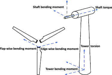
Figure 1: Illustration of structural loads at different components. (The illustration is modified based on a figure originally available at WindData.)

We only study in-land turbines (ILTs) in this work and use the data sets from three ILTs located at different sites. These data sets were collected by Risø-DTU (Technical University of Denmark) [WindData]. Table 1 summarizes the specification of the data sets.

Table 1: Specifications of wind turbines in three data sets

Wind turbine model	NEG-Micon/2750	Vestas V39	Nordtank 500
(Name of data set)	(ILT1)	(ILT2)	(ILT3)
Hub height (m)	80	40	35
Rotor diameter (m)	92	39	41
Cut-in wind speed (m$/$s)	4	4.5	3.5
Cut-out wind speed (m$/$s)	25	25	25
Rated wind speed (m$/$s)	14	16	12
Nominal power (kW)	2750	500	500
Control system	Pitch	Pitch	Stall
Location	Alborg,	Tehachapi Pass,	Roskilde,
	Denmark	California	Denmark
Terrain	Coastal	Bushes	Coastal

We would like to first explain a few terms used in the table as well as in the rest of the paper:

• Pitch control: To avoid production of excessive electricity, turbines hold the rotor at an approximately constant speed in high wind speeds. A pitch controlled turbine turns its blades to regulate its rotor speed.

• Stall control: This serves the same purpose as in pitch control. But the blade angles do not adjust during operation. Instead the blades are designed and shaped to increasingly stall the blade’s angle of attack with the wind to protect the turbine from excessive wind speeds.

• Cut-in wind speed: This is the lowest wind speed at a hub height at which a wind turbine starts to produce power.

• Cut-out wind speed: This is the speed beyond which a wind turbine shuts itself down to protect the turbine.

• Rated wind speed: This is the speed beyond which the turbine’s output power needs to be limited and, consequently, the rotor speeds are regulated, by using, for example, a pitch control mechanism.

Among the structural load responses, we consider only the flap-wise bending moments measured at the root of blades. In other words, $y$ in this study is the 10-minute maximum blade-root flap-wise bending moment (hereafter, we call $y$ a maximum load). But please note that our method applies to other load responses as well. Regarding weather characteristics, since we consider only the ILTs, we include in $\mathbf{x}$ the average wind speed $v$ and the standard deviation of wind speed $s$, namely, $\mathbf{x}:=(v,s)$.

The data are recorded at different frequencies on the ILTs, as follows:

• ILT1: 25 Hz${}={}$15,000 measurements/10-min;

• ILT2: 32 Hz${}={}$19,200 measurements/10-min;

• ILT3: 35.7 Hz${}={}$21,420 measurements/10-min.

Here, 1 Hz means one measurement per second. The raw measured variables are $v_{ij}$ and $y_{ij}$, where $i=1,\ldots,n$ represents a 10-minute block of data and $j=1,\ldots,N$ is the index of the measurements. We use $N$ to represent the number of measurements in a 10-minute block, equal to 15,000, 19,200 and 21,420 for ILT1, ILT2 and ILT3, respectively, and use $n$ to represent the total number of the 10-minute intervals in each data set, taking the value of 1154, 595 and 5688, respectively, for ILT1, ILT2 and ILT3. For these variables, the statistics of the observations in each 10-minute block are calculated as follows:

$$v_{i} = \frac{1}{N}\sum_{j=1}^{N}v_{ij},$$ (4)

$$s_{i} = \sqrt{\frac{1}{N-1}\sum_{j=1}^{N}(v_{ij}-v_{i})^{2}}\quad\mbox{and}$$ (5)

$$y_{i} = \max\{y_{i1},y_{i2},\ldots,y_{iN}\}.$$ (6)

3 Literature review

The previous edition of the international standard, IEC 61400-1:1999, offers a set of design load cases with deterministic wind conditions such as annual average wind speeds, higher and lower turbulence intensities, and extreme wind speeds [IEC (1999)]. In other words, the loads in IEC 61400-1:1999 are specified as discrete events based on design experiences and empirical models [Moriarty, Holley and Butterfield (2002)]. Veers and Butterfield (2001) point out that these deterministic models do not represent the stochastic nature of structure responses, and suggest using statistical modeling to improve design load estimates. Moriarty, Holley and Butterfield (2002) examine the effect of varying turbulence levels on the statistical behavior of a wind turbine’s extreme load. They conclude that the loading on a turbine is stochastic at high turbulence levels, significantly influencing the tail of the load distribution.

In response to these developments, the new edition of IEC 61400-1 standard (IEC 61400-1:2005), issued in 2005, replaces the deterministic load cases with stochastic models, and recommends the use of statistical approaches for determining the extreme load level in the design stage. Freudenreich and Argyriadis (2008) compare the deterministic load cases in the IEC 61400-1:1999 with the stochastic cases in IEC 61400-1:2005, and observe that when statistical approaches are applied, higher extreme load estimates are obtained in some structural responses, such as the blade tip deflection and flap-wise bending moment.

After IEC 61400-1:2005 was issued, many studies were reported to devise and recommend statistical approaches for extreme load analysis [Freudenreich and Argyriadis (2008), Agarwal and Manuel (2008), Peeringa (2009), Moriarty (2008), Fogle, Agarwal and Manuel (2008), Regan and Manuel (2008), Natarajan and Holley (2008)]. These studies adopt a common framework, which we call binning method. The basic idea of the binning method is to discretize the domain of a wind profile vector $\mathbf{x}$ into a finite number of bins. For example, one can divide the range of wind speed, from the cut-in speed to the cut-out speed, into multiple bins and set the width of each bin to, say, 2 m$/$s. Then, in each bin, the conditional short-term distribution of $y|\mathbf{x}$ is approximated by a stationary distribution, with the parameters of the distribution estimated by the method of moments or the maximum likelihood method. Then, the contribution from each bin is summed over all possible bins to determine the final long-term extreme load. In other words, integration in (3) for calculating the long-term distribution is approximated by the summation of finite elements.

According to the classical extreme value theory [Coles (2001), Smith (1990)], the short-term distribution of $y|\mathbf{x}$ can be approximated by a generalized extreme value (GEV) distribution. The probability density function of the GEV is

$$\qquad p(y)=\cases{\displaystyle\frac{1}{\sigma}\exp\biggl{[}-\biggl{(}1+\xi\biggl{(}\frac{y-\mu}{\sigma}\biggr{)}\biggr{)}^{-{1}/{\xi}}\biggr{]}\biggl{(}1+\xi\biggl{(}\frac{y-\mu}{\sigma}\biggr{)}\biggr{)}^{-1-{1}/{\xi}},\vspace*{2pt}\cr\hskip 159.0pt\qquad\mbox{if }\xi\neq 0,\vspace*{2pt}\cr\displaystyle\frac{1}{\sigma}\exp\biggl{[}-\frac{y-\mu}{\sigma}-\exp\biggl{(}-\frac{y-\mu}{\sigma}\biggr{)}\biggr{]},\qquad\mbox{if }\xi=0,}$$ (7)

for $\{y\dvtx 1+\xi(y-\mu)/\sigma>0\}$, where $\mu\in\Re$ is the location parameter, $\sigma>0$ is the scale parameter, and $\xi\in\Re$ is the shape parameter that determines the weight of the tail of the distribution. $\xi>0$ corresponds to the Fréchet distribution with a heavy upper tail, $\xi<0$ to the Weibull distribution with a short upper tail and light lower tail, and $\xi=0$ (or, $\xi\rightarrow 0$) to the Gumbel distribution with a light upper tail [Coles (2001)].

One of the main focuses of interest in extreme value theory is in deriving the quantile value (which, in our study, is defined as the extreme load level $l_{T}$), given the target probability $P_{T}$. The quantile value can be expressed as a function of the distribution parameters as follows:

$$l_{T}=\cases{\displaystyle\mu-\frac{\sigma}{\xi}\bigl{[}1-\bigl{(}-\log(1-P_{T})\bigr{)}^{-\xi}\bigr{]},&\quad$\mbox{if }\xi\neq 0$,\vspace*{2pt}\cr\mu-\sigma\log\bigl{[}-\log(1-P_{T})\bigr{]},&\quad$\mbox{if }\xi=0.$}$$ (8)

The virtue of the binning method is that by modeling the short-term distribution with a homogeneous GEV distribution (i.e., keep the parameters therein constant), it provides a simple way to handle the overall nonstationary load response across different wind speeds. The binning method is perhaps the most common method used in the wind industry and also recommended by IEC (2005). For example, Agarwal and Manuel (2008) use the binning method to estimate the extreme loads for a 2MW offshore wind turbine. In each weather bin, they use the Gumbel distribution to explain the probabilistic behavior of the mudline bending moments of the turbine tower. The data were collected for a period of 16 months. However, most bins have a small number of data, or sometimes, no data at all. For the bins without data, the authors estimate the short-term distribution parameters by using a weighted average of all nonempty bins with the weight related to the inverse squared distance between bins. They quantify the uncertainty of the estimated extreme loads using a bootstrapping technique and report 95% confidence intervals for the short-term extreme load given specific weather conditions (weather bins). Because bootstrapping resamples the existing data for a given weather bin, it cannot precisely capture the uncertainty for those bins with limited data or without data.

Despite its popularity, the binning method has obvious shortcomings in estimating extreme loads. A major limitation is that the short-term load distribution in one bin is constructed separately from the short-term distributions in other bins. This approach requires an enormous amount of data to define the tail of each short-term distribution. In reality, the field data can only be collected in a short duration (e.g., one year out of the 50-year service) and, consequently, some bins do not have enough data. Then, the binning method may end up with inaccuracy or big uncertainty in the estimates of extreme loads. In practice, how many bins to use is also under debate, and there is not yet a consensus. The answer to the action of binning appears to depend on the amount of data—if one has more data, he/she can afford to use more bins; otherwise, fewer bins.

4 Bayesian spline method for extreme load

In this section we present our new procedure of estimating the extreme load with two submodels. The first submodel (in Section 4.1) is the conditional maximum load model $p(y|\mathbf{x})$, and the second submodel (in Section 4.3) is the distribution of wind characteristics $p(\mathbf{x})$. Our major undertaking in this study is on the first submodel, where we present an alternative to the current binning method.

We begin by presenting some scatter plots for the three data sets. Figure 2 shows the scatter plots between the 10-minute maximum loads and 10-minute average wind speeds. We observe nonlinear patterns between the loads and the average wind speeds in all three scatter plots, while individual turbines exhibit different response patterns. ILT1 and ILT2 are two pitch controlled turbines, so when the wind speed reaches or exceeds the rated speed, the blades are adjusted to reduce the absorption of wind energy. As a result, we observe that the loads show a downward trend after the rated wind speed. But different from that of ILT1, the load response of ILT2 has a large variation beyond the rated wind speed. This large variation can be attributed to its less capable control system since ILT2 is one of the early turbine models using a pitch control system. ILT3 is a stall controlled turbine, and its load pattern in Figure 2(c) does not have an obvious downward trend beyond the rated speed.

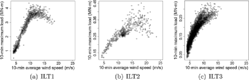
Figure 2: Scatter plots of 10-minute maximum load versus 10-minute average wind speed.

Figure 3 presents the scatter plots between the 10-minute maximum loads and the standard deviations of wind speed during the 10-minute intervals. We also observe nonlinear relationships between them, especially for the new pitch-controlled ILT1. Figure 4 shows scatter plots of 10-minute standard deviation versus 10-minute average wind speed. Some previous studies [Moriarty, Holley and Butterfield (2002), Fitzwater, Cornell and Veers (2003)] suggest that the standard deviation of wind speed varies with the average wind speed, which appears consistent with what we observe in Figure 4.

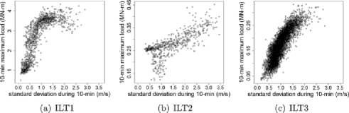
Figure 3: Scatter plots of 10-minute maximum load versus 10-minute standard deviations of wind speed.

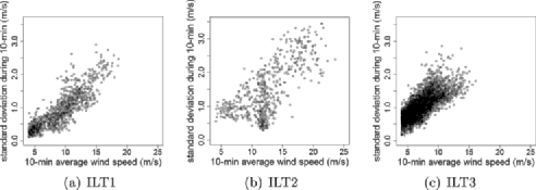
Figure 4: Scatter plots of 10-minute average wind speed versus 10-minute standard deviation of wind speed.

4.1 Submodel 1: Bayesian spline model for conditional maximum load

Recall that in the binning method, a homogeneous GEV distribution is used to model the short-term load distribution, for it appears reasonable to assume stationarity if the chosen weather bin is narrow enough. A finite number of the homogeneous GEV distributions are then stitched together to represent the nonstationary nature across the entire wind profile. What we propose here is to abandon the bins and instead use a nonhomogeneous GEV distribution whose parameters are not constant but depend on weather conditions.

Our research started out with simple approaches based on polynomial models. It turns out that polynomial-based approaches lack the flexibility of adapting to the data sets from different types of turbines. Moreover, due to the nonlinearity around the rated wind speed and the limited amount of data under high wind speeds, polynomial-based approaches performed poorly in those regions that are generally important for capturing the maximum load. Spline models, on the other hand, appear to work better than a global polynomial model, because they have more supporting points spreading over the input regions. In the sequel, we present two flexible Bayesian spline models for the purpose of establishing the desired nonhomogeneous GEV distribution.

Suppose we observe 10-minute maximum loads $y_{1},\ldots,y_{n}$ with corresponding covariate variables $\mathbf{x}_{1}=(v_{1},s_{1}),\ldots,\mathbf{x}_{n}=(v_{n},s_{n})$, as defined in (4) and (5). We choose to model $y_{i}$ with a GEV distribution:

$$y_{i}|\mathbf{x}_{i}\sim\operatorname{GEV}\bigl{(}\mu(\mathbf{x}_{i}),\sigma(\mathbf{x}_{i}),\xi\bigr{)},\qquad\sigma(\cdot)>0,$$ (9)

where the location parameter $\mu$ and scale parameter $\sigma$ in this GEV distribution are a nonlinear function of wind characteristics $\mathbf{x}$. The shape parameter $\xi$ is fixed across the wind profile, while its value will still be estimated using the data from a specific wind turbine. The reason that we keep $\xi$ fixed is to keep the final model from becoming overly complicated. Let us denote $\mu(\mathbf{x}_{i})$ and $\sigma(\mathbf{x}_{i})$ by

$$\mu(\mathbf{x}_{i}) = f(\mathbf{x}_{i}),$$ (10)

$$\sigma(\mathbf{x}_{i}) = \exp\bigl{(}g(\mathbf{x}_{i})\bigr{)},$$ (11)

where in (11), an exponential function is used to ensure the positivity of the scale parameter.

Our strategy of modeling $f(\cdot)$ and $g(\cdot)$ is to use a Bayesian MARS (multivariate adaptive regression splines) model [Denison, Mallick and Smith (1998), Denison et al. (2002)] for capturing the nonlinearity between the load response and the wind-related covariates. The Bayesian MARS model has high flexibility. It includes the number and locations of knots as part of its model parameters and determines these from observed data. In addition, interaction effects among input factors can be modeled if choosing appropriate basis functions.

Specifically, the Bayesian MARS models $f(\mathbf{x})$ for the location parameter $\mu$ and $g(\mathbf{x})$ for the scale parameter $\sigma$ are represented as a linear combination of the basis functions $B^{\mu}_{k}(\mathbf{x})$ and $B^{\sigma}_{k}(\mathbf{x})$, respectively, as

$$f(\mathbf{x}) = \sum_{k=1}^{K_{\mu}}\beta_{k}B^{\mu}_{k}(\mathbf{x}),$$ (12)

$$g(\mathbf{x}) = \sum_{k=1}^{K_{\sigma}}\theta_{k}B^{\sigma}_{k}(\mathbf{x}),$$ (13)

where $\beta_{k},k=1,\ldots,K_{\mu}$ and $\theta_{k},k=1,\ldots,K_{\sigma}$ are the coefficients of the basis functions $B^{\mu}_{k}(\cdot)$ and $B^{\sigma}_{k}(\cdot)$, respectively, and $K_{\mu}$ and $K_{\sigma}$ are the number of the respective basis functions. According to the study by Denison, Mallick and Smith (1998), which proposed the Bayesian MARS, the basis functions are specified as follows:

$$B_{k}(\mathbf{x})=\cases{1,&\quad$k=1$,\vspace*{2pt}\cr\displaystyle\prod_{j=1}^{J_{k}}\bigl{[}h_{jk}\cdot(x_{r(j,k)}-t_{jk})\bigr{]}_{+},&\quad$k=2,3,\ldots,K$.}$$ (14)

Here, $[\cdot]_{+}=\max(0,\cdot)$, $J_{k}$ is the degree of interaction modeled by the basis function $B_{k}(\mathbf{x})$, $h_{jk}$ is the sign indicator, taking the value of either $-1$ or $+1$, and $r(j,k)$ produces the index of the predictor variable which is being split on $t_{jk}$, commonly referred to as the knot points.

We here introduce an integer variable $T_{k}$ to represent the types of basis functions used in (14). Since we consider two predictors $v$ and $s$ for inland turbines, there could be three types of basis functions, namely, $[\pm(v-*)]_{+}$ and $[\pm(s-*)]_{+}$ for each explanatory variable, respectively, and $[\pm(v-*)]_{+}[\pm(s-*)]_{+}$ for interactions between them. So we let $T_{k}$ take the integer value of 1, 2 or 3, to represent the three types of basis functions. That is, $[\pm(v-*)]_{+}$ is represented by $T_{k}=1$, $[\pm(s-*)]_{+}$ represented by $T_{k}=2$, and $[\pm(v-*)]_{+}[\pm(s-*)]_{+}$ represented by $T_{k}=3$. When $J_{k}=1$ in equation (14), then the first two types of basis functions are used, while when $J_{k}=2$, all three types of basis functions are used. In our model, we set $J_{k}=1$ or $J_{k}=2$ in the model of the location parameter $\mu$ for ILT1 and ILT3 data to allow the interaction to be modeled. For ILT2, however, due to its relatively smaller data amount, a model setting $J_{k}=2$ produces unstable and unreasonably wide credible intervals. So for ILT2, $J_{k}=1$ is set for its location parameter $\mu$. For the scale parameter $\sigma$, we set $J_{k}=1$ for all three data sets, but for ILT2, again due to its data scarcity, we include $v$ as the only predictor in its scale parameter model.

Let $\bolds{\Psi}_{a}=(\bolds{\Psi}_{\mu},\bolds{\Psi}_{\sigma},\xi)$ denote all the parameters used in model (9), where $\bolds{\Psi}_{\mu}$ and $\bolds{\Psi}_{\sigma}$ include the parameters in function $f(\cdot)$ and $g(\cdot)$, respectively. These parameters are grouped into two sets: (1) the coefficients of the basis functions in $\bolds{\beta}=(\beta_{1},\ldots,\beta_{K_{\mu}})$ or $\bolds{\theta}=(\theta_{1},\ldots,\theta_{K_{\sigma}})$, and (2) the number and locations of the knots, and the types of basis function in $\bolds{\phi}_{\mu}$ or $\bolds{\phi}_{\sigma}$, as follows:

$$\bolds{\phi}_{\mu}=\bigl{(}K_{\mu},\bolds{\Lambda}^{\mu}_{2},\ldots,\bolds{\Lambda}^{\mu}_{K_{\mu}}\bigr{)},$$

(15)

$$\eqntext{\mbox{where }\bolds{\Lambda}^{\mu}_{k}=\cases{\bigl{(}T^{\mu}_{k},h^{\mu}_{1k},t^{\mu}_{1k}\bigr{)},&\quad$\mbox{when }T^{\mu}_{k}=1,2$;\vspace*{2pt}\cr\bigl{(}T^{\mu}_{k},h^{\mu}_{1k},h^{\mu}_{2k},t^{\mu}_{1k},t^{\mu}_{2k}\bigr{)},&\quad$\mbox{when }T^{\mu}_{k}=3,$}}$$ (16)

and

$$\bolds{\phi}_{\sigma} = \bigl{(}K_{\sigma},\bolds{\Lambda}^{\sigma}_{2},\ldots,\bolds{\Lambda}^{\sigma}_{K_{\sigma}}\bigr{)},$$

$$\eqntext{\mbox{where }\bolds{\Lambda}^{\sigma}_{k}=\bigl{(}T^{\sigma}_{k},h^{\sigma}_{1k},t^{\sigma}_{1k}\bigr{)}\mbox{ when }T^{\sigma}_{k}=1,2.}$$ (18)

Using the above notation, we have $\bolds{\Psi}_{\mu}=(\bolds{\beta},\bolds{\phi}_{\mu})$ and $\bolds{\Psi}_{\sigma}=(\bolds{\theta},\bolds{\phi}_{\sigma})$.

To complete the Bayesian formulation for the model in (9), priors of the parameters involved should be specified. In this paper, we use uniform priors on $\bolds{\phi}_{\mu}$ and $\bolds{\phi}_{\sigma}$; see the detailed expression in Appendix A. Given $\bolds{\phi}_{\mu}$ and $\bolds{\phi}_{\sigma}$, we specify the prior distribution for the parameters $(\bolds{\beta},\bolds{\theta},\xi)$ as the unit-information prior, that is, UIP [Kass and Wasserman (1995)], which is defined by setting the corresponding covariance matrix to be equal to the Fisher information of one observation.

4.2 Submodel 1: Posterior distribution of parameters

The BayesianMARS model treats the number and locations of the knots as random quantities. When the number of knots changes, the dimension of the parameter space changes with it. To handle a varying dimensionality in the probability distributions in a random sampling procedure, researchers usually use a reversible jump Markov chain Monte Carlo (RJMCMC) algorithm developed by Green (1995). The acceptance probability for a RJMCMC algorithm includes a Jacobian term, which accounts for the change in dimension. However, under the assumption that the model space for parameters of varying dimension is discrete, there is no need for a Jacobian. In our analysis, this assumption is satisfied since we only consider probable models over all possible knot locations and numbers. Therefore, instead of using the RJMCMC algorithm, we use the reversible jump sampler (RJS) algorithm proposed in Denison et al. (2002). Since the RJS algorithm does not require new parameters to match dimensions between models and the corresponding Jacobian term to the acceptance probability, it is simpler and more efficient to execute.

To allow for dimensional changes, there are three actions in the RJS algorithm: BIRTH, DEATH and MOVE, which adds, deletes or alters a basis function, respectively. Accordingly, the number of knots as well as the locations of some knots change. The detailed definitions of the three actions are given in Denison et al. (2002), page 53, so we need not repeat them here. They suggest the following: use equal probability (i.e., $\frac{1}{3}$) to propose any of the three moves, and then use the following acceptance probability $\alpha$ for a proposed move from a model having $k$ basis functions to a model having $k^{c}$ basis functions:

$$\alpha=\min\{1,\mbox{the ratio of marginal likelihood }\times R\},$$ (19)

where $R$ is a ratio of probabilities defined as follows:

• For a BIRTH action, $R=\frac{\mbox{probability of DEATH in model $k^{c}$}}{\mbox{probability of BIRTH in model $k$}}$;

• For a DEATH action, $R=\frac{\mbox{probability of BIRTH in model $k^{c}$}}{\mbox{probability of DEATH in model $k$}}$;

• For a MOVE action, $R=\frac{\mbox{probability of MOVE in model $k^{c}$}}{\mbox{probability of MOVE in model $k$}}$.

We have $R=1$ for most cases, because the probabilities in the denominator and numerator are equal, except when $k$ reaches either the upper or the lower bound.

The marginal likelihood in (19) can be expressed as follows:

$$p(\mathcal{D}_{y}|\bolds{\phi}_{\mu},\bolds{\phi}_{\sigma})$$

(20)

$$\qquad=\int{p(\mathcal{D}_{y}|\bolds{\beta},\bolds{\theta},\xi,\bolds{\phi}_{\mu},\bolds{\phi}_{\sigma})p(\bolds{\beta},\bolds{\theta},\xi|\bolds{\phi}_{\mu},\bolds{\phi}_{\sigma})\,d\bolds{\beta}\,d\bolds{\theta}\,d\xi},$$

where $\mathcal{D}_{y}=({y_{1},\ldots,y_{n}})$ represents a set of observed load data. Since it is difficult to calculate the above marginal likelihood analytically in our study, we consider an approximation of $p(\mathcal{D}_{y}|\bolds{\phi}_{\mu},\bolds{\phi}_{\sigma})$. Kass and Wasserman (1995) and Raftery (1995) showed that when UIP priors are used, the marginal log-likelihood, that is, $\log(p(\mathcal{D}_{y}|\bolds{\phi}_{\mu},\bolds{\phi}_{\sigma}))$, can be reasonably approximated by the Schwarz information criterion (SIC) [Schwarz (1978)]. The SIC is expressed as

$$\mathrm{SIC}_{\bolds{\phi}_{\mu},\bolds{\phi}_{\sigma}}=\log\bigl{(}p(\mathcal{D}_{y}|\hat{\bolds{\beta}},\hat{\bolds{\theta}},\hat{\xi},\bolds{\phi}_{\mu},\bolds{\phi}_{\sigma})\bigr{)}-\tfrac{1}{2}\,d_{k}\log(n),$$

where $\hat{\bolds{\beta}},\hat{\bolds{\theta}},\hat{\xi}$ are the maximum likelihood estimators (MLEs) of the corresponding parameters obtained conditional on $\bolds{\phi}_{\mu}$ and $\bolds{\phi}_{\sigma}$, and $d_{k}$ is the total number of parameters to be estimated. In this case, $d_{k}=K_{\mu}+K_{\sigma}+1$.

Recall that we have two dimension-varying states $\bolds{\phi}_{\mu}$ and $\bolds{\phi}_{\sigma}$ in the RJS algorithm. Depending on which state vector is changing, two marginal log-likelihood ratios are needed, and they are approximated by the corresponding SICs, such as

$$\log\frac{p(\mathcal{D}_{y}|\bolds{\phi}_{\mu}^{c},\bolds{\phi}_{\sigma})}{p(\mathcal{D}_{y}|\bolds{\phi}_{\mu},\bolds{\phi}_{\sigma})} \backsimeq \mathrm{SIC}_{\bolds{\phi}^{c}_{\mu},\bolds{\phi}_{\sigma}}-\mathrm{SIC}_{\bolds{\phi}_{\mu},\bolds{\phi}_{\sigma}}\quad\mbox{and}$$ (21)

$$\log\frac{p(\mathcal{D}_{y}|\bolds{\phi}_{\mu},\bolds{\phi}_{\sigma}^{c})}{p(\mathcal{D}_{y}|\bolds{\phi}_{\mu},\bolds{\phi}_{\sigma})} \backsimeq \mathrm{SIC}_{\bolds{\phi}_{\mu},\bolds{\phi}^{c}_{\sigma}}-\mathrm{SIC}_{\bolds{\phi}_{\mu},\bolds{\phi}_{\sigma}}.$$ (22)

Then, we use two acceptance probabilities $\alpha_{\mu}$ and $\alpha_{\sigma}$ for accepting or rejecting a new state in $\bolds{\phi}_{\mu}$ and $\bolds{\phi}_{\sigma}$, respectively. Using the SICs, $\alpha_{\mu}$ and $\alpha_{\sigma}$ are expressed as

$$\alpha_{\mu} = \min\bigl{\{}1,\exp(\mathrm{SIC}_{\bolds{\phi}^{c}_{\mu},\bolds{\phi}_{\sigma}}-\mathrm{SIC}_{\bolds{\phi}_{\mu},\bolds{\phi}_{\sigma}})\times R\bigr{\}}\quad\mbox{and }$$ (23)

$$\alpha_{\sigma} = \min\bigl{\{}1,\exp(\mathrm{SIC}_{\bolds{\phi}_{\mu},\bolds{\phi}^{c}_{\sigma}}-\mathrm{SIC}_{\bolds{\phi}_{\mu},\bolds{\phi}_{\sigma}})\times R\bigr{\}}.$$ (24)

In order to produce the samples from the posterior distribution of parameters in $\bolds{\Psi}_{a}$, we sequentially draw samples for $\bolds{\phi}_{\mu}$ and $\bolds{\phi}_{\sigma}$ by using the two acceptance probabilities, while marginalizing out ($\bolds{\beta}$, $\bolds{\theta}$, $\xi$); and then, conditional on the sampled $\bolds{\phi}_{\mu}$ and $\bolds{\phi}_{\sigma}$, draw samples for ($\bolds{\beta}$, $\bolds{\theta}$, $\xi$) using a Normal approximation based on the maximum likelihood estimates and the observed information matrix. The detailed simulation procedure can be found in Step I of Appendix B.

4.3 Submodel 2: Distribution of wind characteristics

To find a site-specific load distribution, the distribution of wind characteristics $p(\mathbf{x})$ in (3) needs to be specified. Since a statistical correlation is noticed between the 10-minute average wind speed $v$ and the standard deviation of wind speeds $s$ in Figure 4, the distribution of wind characteristics $p(\mathbf{x})$ can be written as a product of the average wind speed distribution $p(v)$ and the conditional wind standard deviation distribution $p(s|v)$. In this section we separately discuss how to specify each model.

For modeling the 10-minute average wind speed $v$, the IEC standard suggests using a 2-parameter Weibull distribution (W2) or a Rayleigh distribution (RAY) [IEC (2005)]. These two distributions are arguably the most widely used ones for this purpose. Carta, Ramirez and Velazquez (2008) and Li and Shi (2010) note that under different wind regimes other distributions may fit wind speed data better, including 3-parameter Weibull distribution (W3), 3-parameter log-Normal distribution (LN3), 3-parameter Gamma distribution (G3) and 3-parameter inverse-Gaussian distribution (IG3). We take a total of six candidate distribution models for average wind speed (W2, W3, RAY, LN3, G3, IG3) from Li and Shi (2010), and conduct a Bayesian model selection to choose the best distribution fitting a given average wind speed data set.

We assume UIP priors for the parameters involved in the aforementioned models, and our approach is again based on maximizing the $\mathrm{SIC}$. Once the best wind speed model is chosen, we denote it by $\mathcal{M}_{v}$. Then, the distribution of 10-minute average wind speed $v$ is expressed as

$$v_{i}\sim\mathcal{M}_{v}(\bolds{\nu}),$$ (25)

where $\bolds{\nu}$ is the set of parameters specifying $\mathcal{M}_{v}$. For instance, if $\mathcal{M}_{v}$ is W3, then $\bolds{\nu}=(\nu_{1},\nu_{2},\nu_{3})$, where $\nu_{1}$, $\nu_{2}$ and $\nu_{3}$ represent the shape, scale and shift parameter, respectively, of a 3-parameter Weibull distribution.

For modeling the standard deviation of wind speed $s$, given the average wind speed $v$, the IEC standard recommends using a 2-parameter Truncated Normal distribution (TN2) [IEC (2005)], which appears to be what researchers have commonly used; see, for example, Fitzwater, Cornell and Veers (2003). The distribution is characterized by a location parameter $\eta$ and a scale parameter $\delta$. In the literature, both $\eta$ and $\delta$ are treated as a constant. But we observe that data sets measured at different sites have different relationships between the average wind speed $v$ and the standard deviation $s$. Some of the $v$-versus-$s$ scatter plots show nonlinear patterns.

Motivated by this observation, we employ a Bayesian MARS model for modeling $\eta$ and $\delta$, similar to what we did in Submodel 1. The standard deviation of wind speed $s$, conditional on the average wind speed $v$, can then be expressed as

$$s_{i}|v_{i}\sim TN2\bigl{(}\eta(v_{i}),\delta(v_{i})\bigr{)},$$

(26)

$$\eqntext{\mbox{where }\eta(v_{i})=f_{\eta}(v_{i})\mbox{ and }\delta(v_{i})=\exp\bigl{(}g_{\delta}(v_{i})\bigr{)},}$$ (27)

where $f_{\eta}$ and $g_{\delta}$, like their counterparts in (12) and (13), are linear combinations of the basis functions taking the general form (14). Notice that both of the functions have only one input variable, which is the average wind speed.

Let $\bolds{\Psi}_{\eta}=(\bolds{\beta}_{\eta},\bolds{\phi}_{\eta})$ and $\bolds{\Psi}_{\delta}=(\bolds{\theta}_{\delta},\bolds{\phi}_{\delta})$ denote the parameters in $f_{\eta}(\cdot)$ and $g_{\delta}(\cdot)$. Since the basis functions $f_{\eta}$ and $g_{\delta}$ in (4.3) have only one input variable, only one type of basis function (i.e., $T_{k}=1$) is needed. Hence, $\bolds{\phi}_{\eta}$ and $\bolds{\phi}_{\delta}$ are much simpler than $\bolds{\phi}_{\mu}$ and $\bolds{\phi}_{\sigma}$, their counterparts in (4.1) and (4.1), and are expressed as follows:

$$\bolds{\phi}_{\eta}=\bigl{(}K_{\eta},\bolds{\Lambda}^{\eta}_{2},\ldots,\bolds{\Lambda}^{\eta}_{K_{\eta}}\bigr{)},$$

(28)

$$\eqntext{\mbox{where }\bolds{\Lambda}^{\eta}_{k}=\bigl{(}T^{\eta}_{k},h^{\eta}_{1k},t^{\eta}_{1k}\bigr{)}\mbox{ and }T^{\eta}_{k}=1}$$ (29)

and

$$\bolds{\phi}_{\delta}=\bigl{(}K_{\delta},\bolds{\Lambda}^{\delta}_{2},\ldots,\bolds{\Lambda}^{\delta}_{K_{\delta}}\bigr{)},$$

(30)

$$\eqntext{\mbox{where }\bolds{\Lambda}^{\delta}_{k}=\bigl{(}T^{\delta}_{k},h^{\delta}_{1k},t^{\delta}_{1k}\bigr{)}\mbox{ and }T^{\delta}_{k}=1.}$$ (31)

We choose the prior distribution for $(\bolds{\beta}_{\eta},\bolds{\theta}_{\delta})$ as UIP and the prior for $(\bolds{\phi}_{\eta},\bolds{\phi}_{\delta})$ as uniform distribution, and solve this Bayesian MARS model by using a RJS algorithm, as in the preceding two sections. The predictive distributions of the average wind speed $\tilde{v}$ and the standard deviation $\tilde{s}$ are

$$p(\tilde{v}|\mathcal{D}_{v}) = \int p(\tilde{v}|\bolds{\nu})p(\bolds{\nu}|\mathcal{D}_{v})\,d\bolds{\nu}\quad\mbox{and}$$ (32)

$$\qquad p(\tilde{s}|\tilde{v},\mathcal{D}_{v},\mathcal{D}_{s}) = \int\int p(\tilde{s}|\tilde{v},\bolds{\Psi}_{\eta},\bolds{\Psi}_{\delta})p(\bolds{\Psi}_{\eta},\bolds{\Psi}_{\delta}|\mathcal{D}_{v},\mathcal{D}_{s})\,d\bolds{\Psi}_{\eta}\,d\bolds{\Psi}_{\delta},$$ (33)

where $\mathcal{D}_{v}$ and $\mathcal{D}_{s}$ are the data sets of the observed average wind speeds and the standard deviations. The detailed simulation procedure is included in Step II in Appendix B.

4.4 Posterior predictive distribution of the extreme load level $l_{T}$

We are interested in getting the posterior predictive distribution of the quantile value $l_{T}$, based on the observed load and wind data $\mathcal{D}:=(\mathcal{D}_{y},\mathcal{D}_{v},\mathcal{D}_{s})$. In order to do so, we need to draw samples $\tilde{y}$’s from the predictive distribution of the maximum load given parameters $p[\tilde{y}|\mathcal{D},\bolds{\Psi}_{a}]$, which is

$$p[\tilde{y}|\mathcal{D},\bolds{\Psi}_{a}]=\int\int p[\tilde{y}|\tilde{v},\tilde{s},\bolds{\Psi}_{a},\mathcal{D}]p[\tilde{v},\tilde{s}|\mathcal{D}_{v},\mathcal{D}_{s}]\,d\tilde{v}\,d\tilde{s},$$ (34)

where $p[\tilde{v},\tilde{s}|\mathcal{D}_{v},\mathcal{D}_{s}]$ can be expressed as the product of (32) and (33).

To calculate a quantile value of the load for a given $P_{T}$ [as in (2)], we go through the following steps:

• Draw samples from the joint posterior predictive distribution $p[\tilde{v},\tilde{s}|\mathcal{D}_{v},\mathcal{D}_{s}]$ of wind characteristics $(\tilde{v},\tilde{s})$ (Step II in Appendix B);

• Draw a set of samples from the posterior distribution of model parameters $\bolds{\Psi}_{a}=(\bolds{\Psi}_{\mu},\bolds{\Psi}_{\sigma},\xi)$; this is realized by employing the RJS algorithm in Section 4.2 (or Step I in Appendix B);

• Given the above samples of wind characteristics and model parameters, we calculate ($\mu,\sigma,\xi$) that are needed in a GEV distribution; this yields a short-term distribution $p[\tilde{y}|\tilde{v},\tilde{s},\bolds{\Psi}_{a}]$;

• Integrating out the wind characteristics $(\tilde{v},\tilde{s})$, obtain the long-term distribution $p[\tilde{y}|\mathcal{D},\bolds{\Psi}_{a}]$;

• Draw samples from $p[\tilde{y}|\mathcal{D},\bolds{\Psi}_{a}]$, and compute a quantile value $l_{T}[\bolds{\Psi}_{a}]$ corresponding to $P_{T}$.

In fact, the predictive mean and Bayesian credible interval of the extreme load level $l_{T}$ are obtained when running the RJS algorithm. The RJS runs through $M_{l}$ iterations and, at each iteration, we obtain a set of samples of the model parameters $\bolds{\Psi}_{a}$ and calculate a $l_{T}[\bolds{\Psi}_{a}]$. Once $M_{l}$ values of $l_{T}[\bolds{\Psi}_{a}]$ are obtained, its mean and credible intervals can then be numerically computed.

Table 2: $\mathrm{SIC}$ for the average wind speed models

Distributions	ILT1	ILT2	ILT3
W2	$-2984$	$-1667$	$-12\mbox{,}287$
W3	$\mathbf{-2941}$	$\mathbf{-1663}$	$\mathbf{-11\mbox{{,}}242}$
RAY	$-3120$	$-1779$	$-13\mbox{,}396$
LN3	$-2989$	$-1666$	$-11\mbox{,}444$
G3	$-2974$	$-1666$	$-11\mbox{,}290$
IG3	$-2986$	$-2313$	$-11\mbox{,}410$

5 Results

5.1 Model selection

Table 2 presents the $\mathrm{SIC}$ values of the six candidate average wind speed models using different ILT data sets. The boldfaced values indicate the largest $\mathrm{SIC}$ for a given data set and, consequently, the corresponding models are chosen for that data set.

Regarding the average wind speed model, all candidate distributions except RAY provide generally a good model fit for ILT1, with a similar level of fitting quality, but W3 dominates slightly. For the ILT2 data, W2, W3, LN3 and G3 produce similar $\mathrm{SIC}$ values. In the ILT3 data, W3, LN3, G3 and IG3 perform similarly. Still W3 is slightly better. So we choose W3 as our average wind speed model.

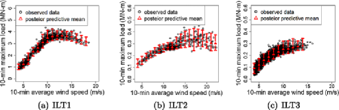
Figure 5: 95% point-wise credible intervals for different wind speeds.

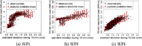
Figure 6: 95% point-wise credible intervals for different standard deviations.

5.2 Point-wise credible intervals

As a form of checking the conditional maximum load model, we present in Figures 5 and 6 the 95% point-wise credible intervals under different wind speeds and standard deviations. To generate these figures, we take a data set and fix $v$ or $s$ at one specific speed or standard deviation at a time and then draw the posterior samples for $\tilde{y}$ from the posterior predictive distribution of conditional maximum load, $p(\tilde{y}|\mathbf{x})$. Suppose that we want to generate the credible intervals at wind speed $v_{*}$ or standard deviation $s_{*}$. The posterior predictive distributions are computed as follows:

$$p\bigl{(}\tilde{y}|(v,s)\in\mathcal{D}_{v_{*}},\mathcal{D}_{y}\bigr{)} = \int p\bigl{(}\tilde{y}|(v,s)\in\mathcal{D}_{v_{*}},\bolds{\Psi}_{a}\bigr{)}p(\bolds{\Psi}_{a}|\mathcal{D}_{y})\,d\bolds{\Psi}_{a},$$

$$p\bigl{(}\tilde{y}|(v,s)\in\mathcal{D}_{s_{*}},\mathcal{D}_{y}\bigr{)} = \int p\bigl{(}\tilde{y}|(v,s)\in\mathcal{D}_{s_{*}},\bolds{\Psi}_{a}\bigr{)}p(\bolds{\Psi}_{a}|\mathcal{D}_{y})\,d\bolds{\Psi}_{a},$$

where $\mathcal{D}_{v_{*}}$ and $\mathcal{D}_{s_{*}}$ are subsets of the observed data such that $\mathcal{D}_{v_{*}}=\{(v_{i},s_{i})\dvtx\break v_{*}-0.5<v_{i}<v_{*}+0.5,\mbox{ and }(v_{i},s_{i})\in\mathcal{D}_{v,s}\}$ and $\mathcal{D}_{s_{*}}=\{(v_{i},s_{i})\dvtx s_{*}-0.05<s_{i}<s_{*}+0.05,\mbox{ and }(v_{i},s_{i})\in\mathcal{D}_{v,s}\}$. Given these distributions, samples for $\tilde{y}$ are drawn to construct the $95\%$ credible intervals at $v_{*}$ or $s_{*}$. The result is shown as one vertical bar in either a $v$-plot (Figure 5) or a $s$-plot (Figure 6). To complete these figures, the process is repeated in the $v$-domain with 1 m$/$s increment and in the $s$-domain with 0.2 m$/$s increment. These figures show that the variability in data are reasonably captured by the spline method.

5.3 Comparison between the binning method and spline method for conditional maximum load

In our procedure for estimating the extreme load level, two different distributions of maximum load $y$ are involved: one is the conditional maximum load distribution $p(y|\mathbf{x})$, aka the short-term distribution, and the other is the unconditional maximum load distribution $p(y)$, aka the long-term distribution. Using the observed field data, it is difficult to assess the estimation accuracy of the extreme load levels in the long-term distribution, because of the relatively small amount of observation records. What we undertake in this section is to evaluate a method’s performance of estimating the tail of the short-term distribution $p(y|\mathbf{x})$. We argued before that the short-term distribution underlies the difference between the proposed Bayesian spline method and the binning method. The comparison in this section is intended to show the advantage of the Bayesian spline method. In Section 5.5 we employ a simulation study that generates a much larger data set, allowing us to compare the performance of two methods in estimating the extreme load level in the long-term distribution.

To evaluate the tail part of a conditional maximum load distribution, we compute a set of upper quantile estimators and assess their estimation qualities using the generalized piecewise linear (GPL) loss function [Gneiting (2011)]. A GPL is defined as follows:

$$S_{\tau,b}\bigl{(}\hat{l}(\mathbf{x}_{i}),y(\mathbf{x}_{i})\bigr{)}$$

$$\qquad=\cases{\displaystyle\bigl{(}\mathbh{1}{\bigl{(}\hat{l}(\mathbf{x}_{i})\geq y(\mathbf{x}_{i})\bigr{)}}-\tau\bigr{)}\frac{1}{|b|}\bigl{(}\bigl{[}\hat{l}(\mathbf{x}_{i})\bigr{]}^{b}-\bigl{[}y(\mathbf{x}_{i})\bigr{]}^{b}\bigr{)},&\quad$\mbox{for }b\neq{0}$,\vspace*{2pt}\cr\displaystyle\bigl{(}\mathbh{1}{\bigl{(}\hat{l}(\mathbf{x}_{i})\geq y(\mathbf{x}_{i})\bigr{)}}-\tau\bigr{)}\log{\biggl{(}\frac{\hat{l}(\mathbf{x}_{i})}{y(\mathbf{x}_{i})}\biggr{)}},&\quad$\mbox{for }b={0},$}$$

where $\hat{l}(\mathbf{x}_{i})$ is the $\tau$-quantile estimation of $p(y|\mathbf{x}_{i}$) for a given $\mathbf{x}_{i}$, $y(\mathbf{x}_{i})$ is the observed maximum load in the test data set, given the same $\mathbf{x}_{i}$, $b$ is a power parameter, and $\mathbh{1}$ is an indicator function. The power parameter $b$ usually ranges between 0 and 2.5. When $b=1$, the GPL loss function is the same as the piecewise linear (PL) loss function.

For the above empirical evaluation, we randomly divide a data set into a partition of 80% for training and 20% for testing. We use the training set to establish a short term distribution $p(y|\mathbf{x}$). For any $\mathbf{x}_{i}$ in the test set, the $\tau$-quantile estimation $\hat{l}(\mathbf{x}_{i})$ can be computed using $p(y|\mathbf{x}$). And then, the GPL loss function value is taken as the average of all $S_{\tau,b}$ values over the test set, as follows:

$$\overline{S}_{\tau,b}=\frac{1}{n_{t}}\sum_{i=1}^{n_{t}}S_{\tau,b}\bigl{(}\hat{l}_{i}(\mathbf{x}_{i}),y_{i}\bigr{)},$$ (36)

where $n_{t}$ is the number of data points in a test set and $y_{i}$ is the same as $y(\mathbf{x}_{i})$. We call $\overline{S}_{\tau,b}$ the mean score. We repeat the training/test procedure 10 times, and the final mean score is the average of the ten mean scores. For notational simplicity, we still call the final mean score the mean score and use $\overline{S}_{\tau,b}$ to represent it, as long as its meaning is clear in the context.

In this comparison, we use two methods to establish the short-term distribution: the binning method and the proposed Bayesian spline method. In our RJS algorithm in Section 4.2, we draw $N_{l}=100$ samples from the short-term distribution. Accordingly, we can evaluate the quality of quantile estimations of the short-term distribution for a $\tau$ up to $0.99$.

We first take a look at the comparisons in Figure 7, which compares the PL loss (i.e., $b=1$) of both methods as $\tau$ varies in the above-mentioned range. The left vertical axis shows the values of the mean score of the PL loss, while the right axis is the percentage value of the reduction in mean scores when the spline method is compared with the binning method. For all three data sets, the spline method maintains lower mean scores than the binning method.

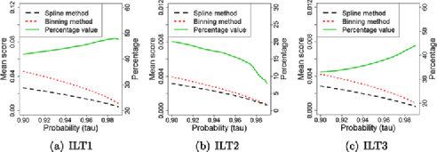
Figure 7: Comparison of PL function: the left Y-axis represents the mean score values and the right Y-axis represents the percentage values, which are the reduction in the mean scores when the spline method is compared with the binning method.

When $\tau$ is approaching $0.99$ in Figure 7, it looks like the PL losses of the spline and binning methods are getting closer to each other. This is largely due to the fact that the PL loss values are smaller at a higher $\tau$, so that their differences are compressed in the figure. If one looks at the solid line in a plot, which represents the percentage of reduction in the mean score, the spline method’s advantage over the binning method is more evident in the cases of ILT1 and ILT3 data sets. When $\tau$ gets larger, the spline method produces a significant improvement over the binning method, with a reduction of PL loss ranging from $33\%$ to $50\%$. The trend is different when using the ILT2 data set. But still, the spline method can reduce the mean scores of the PL loss from the binning method by $8\%$ to $20\%$. Please note that the ILT2 data set is the smallest set, having slightly fewer than 600 data records. We believe that the difference observed over the ILT2 case is attributable to the scarcity of data.

We compute the mean scores of the GPL loss under three different power parameters $b=0,1,2$ for each method. Table 3 presents the results under $\tau=0.9$, while Table 4 is for $\tau=0.99$. In Table 3 the spline method has a mean score 20% to 42% lower than the binning method. In Table 4 the reductions in mean scores are in a similar range. Overall, these results clearly show the improvement achieved by employing the Bayesian spline method.

Table 3: Mean scores of GPL/PL for the $0.9$-quantile estimators

	ILT1		ILT2		ILT3
Power parameter	Binning	Spline	Binning	Spline	Binning	Spline
$b=0$	0.0185	0.0108	0.0129	0.0103	0.0256	0.0171
$b=1$	0.0455	0.0265	0.0040	0.0031	0.0042	0.0028
$b=2$	0.1318	0.0782	0.0013	0.0010	0.0008	0.0005

Table 4: Mean scores of GPL/PL for the $0.99$-quantile estimators

	ILT1		ILT2		ILT3
Power parameter	Binning	Spline	Binning	Spline	Binning	Spline
$b=0$	0.0031	0.0018	0.0022	0.0020	0.0045	0.0027
$b=1$	0.0086	0.0045	0.0007	0.0006	0.0008	0.0005
$b=2$	0.0270	0.0135	0.0003	0.0002	0.0002	0.0001

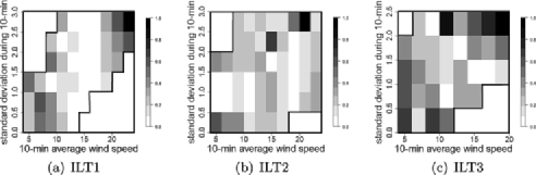
Figure 8: Comparison of the $0.99$-quantiles between binning method and spline method.

In order to understand the difference between the spline method and binning method, we compare the $0.99$ quantiles of the 10-minute maximum load conditional on a specific wind condition. This is done by computing the difference in the quantile values of the conditional maximum load from the two methods for different weather bins. The wind condition of each bin is approximated by the median values of $v$ and $s$ in that bin. Figure 8 shows the standardized difference of the two $0.99$ quantile values in each bin. The darker the color is, the bigger the difference. Note that we exclude comparisons in the weather bins with very low likelihood, namely, low wind speed and high standard deviation or high wind speed and low standard deviation.

Table 5: Estimates of extreme load levels ($l_{T},T=20$ years), unit: MN-m

Data sets	Binning method	Spline method
ILT1	6.455 (6.063, 7.092)	4.750 (4.579, 4.955)
ILT2	0.752 (0.658, 0.903)	0.576 (0.538, 0.627)
ILT3	0.505 (0.465, 0.584)	0.428 (0.398, 0.463)

Table 6: Estimates of extreme load level ($l_{T},T=50$ years), unit: MN-m

Data sets	Binning method	Spline method
ILT1	6.711 (6.240, 7.485)	4.800 (4.611, 5.019)
ILT2	0.786 (0.682, 0.957)	0.589 (0.547, 0.646)
ILT3	0.527 (0.480, 0.621)	0.438 (0.405, 0.476)

We can observe that the two methods produce similar results at the bins having a sufficient number of data points (mostly weather bins in the central area), and the results are different when the data are scarce—this tends to happen at the two ends of the average wind speed and standard deviation. This echoes the point we made earlier that without binning the weather conditions, the spline method is able to make better use of the available data and overcome the limited data problem for rare weather events.

5.4 Estimation of extreme load

Finally, Tables 5 and 6 show the estimates of the extreme load levels $l_{T}$, corresponding to $T=20$ and $T=50$ years, respectively. The values in parenthesis are the 95% credible (or confidence) intervals.We observe that the extreme load levels $l_{T}$ obtained by the binning method are generally higher than those obtained by the spline method. This should not come as a surprise. As we push for a high quantile, more data would be needed in each weather bin, but the amounts in reality are limited due to the binning method’s compartmentalization of data. The binning method also produces a wider confidence interval than the spline method, as a result of the same rigidity in data handling. The detailed procedure for computing the binning method’s confidence interval is included in Appendix C.

5.5 Simulation of extreme load

In this section a simulation study is undertaken to assess the estimation accuracy of extreme load level in the long-term distribution. The simulations use one single covariate $x$, mimicking the wind speed, and a dependent variable $y$, corresponding to the maximum load. We use the following procedure to generate the simulated data:

[(a)]

Generate a sample $x_{i}$ from a 3-parameter Weibull distribution. Then sample $x_{ij}$, $j=1,\ldots,1000$, from a normal distribution having $x_{i}$ as its mean and a unit variance. The set of $x_{ij}$’s represents the different wind speeds within a bin.

Draw the samples $y_{ij}$ from a normal distribution with its mean as $\mu^{s}_{ij}$ and its standard deviation as $\sigma^{s}_{ij}$, which are expressed as follows:

$$\mu^{s}_{ij} = \cases{\displaystyle\frac{1.5}{[1+48\times\exp(-0.3\times x_{ij})]},\vspace*{2pt}\cr\qquad\mbox{if }x_{i}<17,\vspace*{2pt}\cr\displaystyle\frac{1.5}{[1+48\times\exp(-0.3\times x_{ij})]}+\bigl{[}0.5-0.0016\times\bigl{(}x_{i}+x_{i}^{2}\bigr{)}\bigr{]},\vspace*{2pt}\cr\qquad\mbox{if }x_{i}\geq 17,}$$

$$\sigma^{s}_{ij} = 0.1\times\log(x_{ij}).$$

The above set of equations is used to create a $y$ response resembling the load data we observe. The parameters used in the equations are chosen through trials so that the simulated $y$ looks like the actual mechanical load response. While many of the parameters used above do not have any physical meaning, some of them do, for instance, the “$17$” in “$x_{i}<17$” bears the meaning of the rated wind speed.

Find the maximum value $y_{i}=\max\{y_{i,1},\ldots,y_{i,1000}\}$, corresponding to $x_{i}$. According to the classical extreme value theory [Coles (2001), Smith (1990)], $y_{i}$ produced in such a way can be modeled by a GEV distribution.

Repeat (a) through (c) for $i=1,\ldots,1000$ to produce the training data set with $n=1000$ data pairs, and denote this data set by $\mathcal{D}_{\mathrm{TR}}=\{(x_{1},y_{1}),\ldots,(x_{1000},y_{1000})\}$.

Once the training data set $\mathcal{D}_{\mathrm{TR}}$ is simulated, both the binning method and spline method are used to estimate the extreme load levels $l_{T}$ corresponding to two probabilities: $0.0001$ and $0.00001$. This estimation is based on drawing samples from the long-term distribution of $y$, as described in Section 4.4, which produces the posterior predictive distribution of $l_{T}$. To compare the estimation accuracy of the extreme quantile values, we also generate 100 simulated data sets; each data set consists of $100\mbox{,}000$ data points, which are obtained by repeating the above (a) through (c). For each data set, we find the observed quantile values $l_{0.0001}$ and $l_{0.00001}$. Using the 100 simulated data sets, we also obtain 100 different samples of these quantiles.

Figure 9(a) shows a scatter plot of the simulated $x$’s and $y$’s in $\mathcal{D}_{\mathrm{TR}}$, which resembles the load responses we saw previously. Figure 9(b) and (c) present the extreme load levels estimated by the two methods as well as the observed extreme quantile values under the two selected probabilities. We observe that the binning method tends to overestimate the extreme quantile values and yields wider confidence intervals than the spline method. Furthermore, the degree of overestimation appears to increase as the probability corresponding to an extreme quantile value goes smaller. This observation confirms what we observed in Section 5.4 using the field data. This simulation result suggests that using the binning method for extreme load estimation is not a good practice.

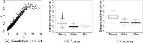
Figure 9: Simulation data set, estimated and observed extreme quantile values: (a) An example of a simulated data set. (b) and (c) Boxplots for the distribution of the binning estimate, the Bayesian spline estimate and the respective sample quantile across 100 simulated data sets.

6 Summary

This study presents a Bayesian spline method for estimating the extreme load on wind turbines. The spline method essentially supports a nonhomogeneous GEV distribution to capture the nonlinear relationship between the load response and the wind-related covariates. Such treatment avoids binning the data. The underlying spline models instead connect all the bins across the whole wind profile, so that load and wind data are pooled together to produce better estimates. This is demonstrated by applying the spline method to three sets of inland wind turbine load response data and making comparisons with the binning method.

The popularity of the binning method in industrial practice is due to the simplicity of its idea and procedure. However, simplicity of a procedure should not be mistaken as simplicity of a model. Suppose that one uses a $6\times 10$ grid to bin the two-dimensional wind covariates (as we did in this study) and fixes the shape parameter $\xi$ across the bins (a common practice in the industry). The binning method yields $60$ local GEV distributions, each of which has two parameters, translating to a total of 121 parameters for the overall model (counting the fixed $\xi$ as well). By contrast, the spline method, although conceptually and procedurally more involved, produces an overall model with fewer parameters. To see this, consider the following: for the three ILT data sets, the average ($K_{\mu}+K_{\sigma}$) from the RJS algorithm is between $12$ and $18$. The number of model parameters $d_{k}$ in (4.2) is generally less than $20$, a number far smaller than the number of parameters in the binning method. In the end, the spline method uses a sophisticated procedure to find a simpler model that is more capable.

Appendix A Priors

In this appendix we specify priors for parameters used in the basis functions as follows:

$$\bolds{\phi} = (K,\bolds{\Lambda}_{2},\ldots,\bolds{\Lambda}_{K})$$

$$\eqntext{\mbox{where }\bolds{\Lambda}_{k}=\cases{(T_{k},h_{1k},t_{1k}),&\quad$\mbox{when }T_{k}=1,2$,\vspace*{2pt}\cr(T_{k},h_{1k},h_{2k},t_{1k},t_{2k}),&\quad$\mbox{when }T_{k}=3,$}}$$ (38)

$$p(K) = \frac{1}{n},\qquad K=\{1,\ldots,n\},$$

$$p(T_{k}) = \cases{1,&\quad$T_{k}=\{1\},\mbox{for }\bolds{\phi}_{\eta}\mbox{ and }\bolds{\phi}_{\delta}$,\vspace*{2pt}\cr\frac{1}{2},&\quad$T_{k}=\{1,2\},\mbox{for }\bolds{\phi}_{\mu}\mbox{ in ILT2 and all }\bolds{\phi}_{\sigma}$,\vspace*{2pt}\cr\frac{1}{3},&\quad$T_{k}=\{1,2,3\},\mbox{for }\bolds{\phi}_{\mu}\mbox{ in ILT1 and ILT3},$}$$

$$p(h_{\cdot k}) = \tfrac{1}{2},\qquad h_{\cdot k}=\{+1,-1\},$$

$$p(t_{\cdot k}) = \frac{1}{n},\qquad t_{\cdot k}=\{v_{1},\ldots,v_{n}\}\mbox{ or }\{s_{1},\ldots,s_{n}\}.$$

Appendix B Implementation details of the spline method

In this appendix we provide the detailed implementation procedure for the spline method. The procedure consists of two major steps: (1) Step I: construct the posterior predictive distribution of the extreme load level $l_{T}$ and (2) Step II: obtain the joint posterior predictive distribution of wind characteristics $(v,s)$.

1. Step I: construct the posterior predictive distribution of the extreme load level using the Bayesian spline models:

   1. [(a)]

   2. Set $t=0$ and the initial $\bolds{\phi}^{(t)}_{\mu}$ and $\bolds{\phi}^{(t)}_{\sigma}$ both to be a constant scalar.

   3. At iteration $t$, $K_{\mu}$ and $K_{\sigma}$ are equal to the number of basis functions specified in $\bolds{\phi}^{(t)}_{\mu}$ and $\bolds{\phi}^{(t)}_{\sigma}$. Find the MLEs of $\bolds{\beta}^{(t)},\bolds{\theta}^{(t)},\xi^{(t)}$ and the inverse of the negative of Hessian matrix, given $\bolds{\phi}^{(t)}_{\mu}$ and $\bolds{\phi}^{(t)}_{\sigma}$.

   4. Generate $u^{1}_{\mu}$ uniformly on $[0,1]$ and choose a move in the RJS procedure. In the following, $b_{K_{\mu}},r_{K_{\mu}},m_{K_{\mu}}$ are the proposal probabilities associated with a move type, and they are all set as $\frac{1}{3}$:

      • If $(u^{1}_{\mu}\leq b_{K_{\mu}})$, then go to BIRTH step, denoted by $\bolds{\phi}_{\mu}^{*}=$ BIRTH-proposal$(\bolds{\phi}_{\mu}^{(t)})$, which is to augment $\bolds{\phi}_{\mu}^{(t)}$ with a $\bolds{\Lambda}^{\mu}_{K_{\mu}+1}$ that is selected uniformly at random;

      • Else if $(b_{K_{\mu}}\leq u^{1}_{\mu}\leq b_{K_{\mu}}+r_{K_{\mu}})$, then go to DEATH step, denoted by $\bolds{\phi}_{\mu}^{*}=$ DEATH-proposal$(\bolds{\phi}_{\mu}^{(t)})$, which is to remove from $\bolds{\phi}_{\mu}^{(t)}$ with a $\bolds{\Lambda}^{\mu}_{k}$ where $2\leq k\leq K_{\mu}$ is selected uniformly at random;

      • Else, go to MOVE step, denoted by $\bolds{\phi}_{\mu}^{*}=$MOVE-proposal$(\bolds{\phi}_{\mu}^{(t)})$, which first does $\bolds{\phi}_{\mu}^{{\dagger}}$ = DEATH-proposal$(\bolds{\phi}_{\mu}^{(t)})$ and then does $\bolds{\phi}_{\mu}^{*}$ = BIRTH-proposal$(\bolds{\phi}_{\mu}^{{\dagger}})$.

   5. Find the MLEs ($\bolds{\beta}^{*},\bolds{\theta}^{*},\xi^{*}$) and the inverse of the negative of Hessian matrix, given $\bolds{\phi}^{*}_{\mu}$ and $\bolds{\phi}_{\sigma}$.

   6. Generate $u^{2}_{\mu}$ uniformly on $[0,1]$ and compute the acceptance ratio $\alpha_{\mu}$ in (23), using the results from (b) and (d).

   7. Accept $\bolds{\phi}_{\mu}^{*}$ as $\bolds{\phi}_{\mu}^{(t+1)}$ with probability $\min(\alpha_{\mu},1)$. If $\bolds{\phi}_{\mu}^{*}$ is not accepted, let $\bolds{\phi}_{\mu}^{(t+1)}=\bolds{\phi}_{\mu}^{(t)}$.

   8. Generate $u_{\sigma}^{1}$ uniformly on $[0,1]$ and choose a move in the RJS procedure. In the following, $b_{K_{\sigma}},r_{K_{\sigma}},m_{K_{\sigma}}$ are the proposal probabilities associated with a move type, and they are all set as $\frac{1}{3}$:

      • If $(u_{\sigma}^{1}\leq b_{K_{\sigma}})$, then go to BIRTH step, denoted by $\bolds{\phi}_{\sigma}^{*}=$ BIRTH-proposal$(\bolds{\phi}_{\sigma}^{(t)})$, which is to augment $\bolds{\phi}_{\sigma}^{(t)}$ with a $\bolds{\Lambda}^{\sigma}_{K_{\sigma}+1}$ that is selected uniformly at random;

      • Else if $(b_{K_{\sigma}}\leq u^{1}_{\sigma}\leq b_{K_{\sigma}}+r_{K_{\sigma}})$, then go to DEATH step, denoted by $\bolds{\phi}_{\sigma}^{*}=$ DEATH-proposal$(\bolds{\phi}_{\sigma}^{(t)})$, which is to remove from $\bolds{\phi}^{(t)}$ with a $\bolds{\Lambda}^{\sigma}_{k}$ where $2\leq k\leq K_{\sigma}$ that is selected uniformly at random;

      • Else, go to MOVE step, denoted by $\bolds{\phi}_{\sigma}^{*}=$MOVE-proposal$(\bolds{\phi}_{\sigma}^{(t)})$, which first does $\bolds{\phi}_{\sigma}^{{\dagger}}$ = DEATH-proposal$(\bolds{\phi}^{(t)})$ and then does $\bolds{\phi}_{\sigma}^{*}$ = BIRTH-proposal$(\bolds{\phi}_{\sigma}^{{\dagger}})$.

   9. Find the MLEs ($\bolds{\beta}^{*},\bolds{\theta}^{*},\xi^{*}$) and the inverse of the negative of Hessian matrix, given $\bolds{\phi}^{t+1}_{\mu}$ and $\bolds{\phi}^{*}_{\sigma}$.

   10. Generate $u_{\sigma}^{2}$ uniformly on $[0,1]$ and compute the acceptance ratio $\alpha_{\sigma}$ in (24), using the results from (d) and (h).

   11. Accept $\bolds{\phi}_{\sigma}^{*}$ as $\bolds{\phi}_{\sigma}^{(t+1)}$ with probability $\min(\alpha_{\sigma},1)$. If $\bolds{\phi}_{\sigma}^{*}$ is not accepted, let $\bolds{\phi}_{\sigma}^{(t+1)}=\bolds{\phi}_{\sigma}^{(t)}$.

   12. After initial burn-ins (in our implementation, initial burn-in is 1000), draw a posterior sample of $(\bolds{\beta}^{(t+1)},\bolds{\theta}^{(t+1)},\xi^{(t+1)})$ from the approximated multivariate normal distribution at the maximum likelihood estimates and the inverse of the negative of the Hessian matrix. Depending on the acceptance or rejection that happened in (f) and (j), the MLEs to be used are obtained from either (b), (d) or (h).

   13. Take the posterior sample of $\bolds{\Psi}_{a}$, obtained in (f), (j) and (k), and calculate a sample of $\mu$ and $\sigma$ using (12) and (13), respectively, for each pair of the $N_{w}\times N_{sw}$ samples of ($v,s$) obtained in Step II. This generates $N_{w}\times N_{sw}$ samples of $\mu$ and $\sigma$.

   14. Draw $N_{l}$ samples for the 10-minute maximum load $\tilde{y}$ from each GEV distribution with $\mu_{i}$, $\sigma_{i}$ and $\xi_{i}$, $i=1,\ldots,N_{w}\times N_{sw}$, where $\mu_{i}$ and $\sigma_{i}$ are among $N_{w}\times N_{sw}$ samples obtained in (l), and $\xi_{i}$ is always set as $\xi^{(t+1)}$.

   15. Get the quantile value (i.e., the extreme load level $l_{T}[\bolds{\Psi}_{a}]$) corresponding to $1-P_{T}$ from the $N_{w}\times N_{sw}\times N_{l}$ samples of $\tilde{y}$.

   16. To obtain a credible interval for $l_{T}$, repeat (b) through (n) $M_{l}$ times.

2. Step II: obtain the joint posterior predictive distribution of wind characteristics $(v,s)$:

   1. [(a)]

   2. Find the MLEs of $\bolds{\nu}$ for all candidate distributions listed in Section 4.3.

   3. Use the $\mathrm{SIC}$ to select the “best” distribution model for the average wind speed $v$. The chosen distribution is used in the subsequent steps to draw posterior samples.

   4. Draw a posterior sample of $\bolds{\nu}$ from the approximated multivariate normal distribution at the MLEs and the inverse of the negative of the Hessian matrix.

   5. Draw $N_{w}$ samples of $\tilde{v}$ using the distribution chosen in (b) with the parameter sampled in (c).

   6. Implement the RJS algorithm again, namely, (a) through (k) in Step I, to get one posterior sample of $\bolds{\Psi}_{\eta}=(\bolds{\beta}_{\eta},\bolds{\phi}_{\eta})$ and $\bolds{\Psi}_{\delta}=(\bolds{\theta}_{\delta},\bolds{\phi}_{\delta})$.

   7. Take the posterior sample of $\bolds{\Psi}_{\eta}$ and $\bolds{\Psi}_{\delta}$, obtained in (e), and calculate a sample of $\eta$ and $\delta$ using (4.3) for each sample of $v$. This generates $N_{w}$ samples of $\eta$ and $\delta$.

   8. Draw a sample for the standard deviation of wind speed $\tilde{s}$ from each truncated normal distribution with $\eta_{i}$, $\delta_{i}$, $i=1,\ldots,N_{w}$. Using the $N_{w}$ samples of $\eta$ and $\delta$ obtained in (f), we obtain $N_{w}$ samples of $\tilde{s}$.

   9. To get $M_{w}\times N_{w}$ samples of $\tilde{v}$ and $\tilde{s}$, repeat (c) through (g) $M_{w}$ times.

In our implementation, we use $M_{w}=1000$, $M_{l}=10\mbox{,}000$, $N_{w}=100$ and $N_{l}=100$.

Appendix C Confidence intervals for the binning method

To calculate the confidence intervals for the binning method, we follow a procedure similar to the one used for calculating the credible intervals in the spline method. The difference is mainly that in the binning method, the parameters used in the GEV distribution, namely, $\mu$ and $\sigma$ (recall that $\xi$ is fixed as a constant across all the bins), are sampled using only the data in a specific bin. For those bins which do not have data, its $\mu$ and $\sigma$ are a weighted average of all nonempty bins with the weight related to the inverse squared distance between bins, following the approach used by Agarwal and Manuel (2008). Once a sample of $\mu$ and $\sigma$ is obtained for a specific bin, the resulting local GEV is used to sample $\tilde{y}$ in that bin. Do this for all the bins, and $\tilde{y}$’s from all bins are pooled together to estimation $l_{T}$.

Specially, we go through the following steps, where $\bolds{\Phi}_{c}$ denotes the collection of the parameters associated with all local GEV distributions used in all bins:

• Draw $M_{w}\times N_{w}$ samples from the joint posterior predictive distribution $p[\tilde{v},\tilde{s}|\mathcal{D}_{v},\mathcal{D}_{s}]$ of wind characteristics $(\tilde{v},\tilde{s})$; this step is the same as in the spline method;

• Using the data in a bin, draw a sample of $\mu$ and $\sigma$ for that specific bin from a multivariate normal distributions taking the MLE as its mean and the inverse of the negative of the Hessian matrix as its covariance matrix. Not all the bins have data. For those which do not have data, its $\mu$ and $\sigma$ are a weighted average of all nonempty bins with the weight related to the inverse squared distance between bins, as we explained above. Collectively, $\bolds{\Phi}_{c}$ contains all the $\mu$’s and $\sigma$’s from all the bins;

• Decide which bins the wind characteristic samples $(\tilde{v},\tilde{s})$’s fall into. Based on the specific bin in which a sample of $(\tilde{v},\tilde{s})$ falls, the corresponding $\mu$ and $\sigma$ in $\bolds{\Phi}_{c}$ is chosen; doing this yields the short-term distribution $p[\tilde{y}|\tilde{v},\tilde{s},\bolds{\Phi}_{c}]$ for that specific bin;

• Draw $N_{l}$ samples of $\tilde{y}$ from $p[\tilde{y}|\tilde{v},\tilde{s},\bolds{\Phi}_{c}]$ for each of the total $M_{w}\times N_{w}$ samples of $(\tilde{v},\tilde{s})$. This produces a total of $M_{w}\times N_{w}\times N_{l}$ $\tilde{y}$ samples;

• One can then compute the quantile value $l_{T}[\bolds{\Phi}_{c}]$ corresponding to $P_{T}$;

• Repeat the above procedure $M_{l}$ times to get the median and confidence intervals of $l_{T}$.

Our implementation here uses the same $M_{w},M_{l},N_{w}$ and $N_{l}$ as those used in the spline method’s implementation.

References

- Agarwal and Manuel (2008) {barticle}[author] \bauthor\bsnmAgarwal, \bfnmP.\binitsP. and \bauthor\bsnmManuel, \bfnmL.\binitsL. (\byear2008). \btitleExtreme loads for an offshore wind turbine using statistical extrapolation from limited field data. \bjournalWind Energy \bvolume11 \bpages673–684. \bptokimsref \endbibitem
- Bottasso, Campagnolo and Croce (2010) {bmisc}[author] \bauthor\bsnmBottasso, \bfnmC. L.\binitsC. L., \bauthor\bsnmCampagnolo, \bfnmF.\binitsF. and \bauthor\bsnmCroce, \bfnmA.\binitsA. (\byear2010). \bhowpublishedComputational procedures for the multi-disciplinary constrained optimization of wind turbines. Technical report, Dipartimento di Ingegneria Aerospaziale. Available at http://www.aero.polimi.it/~bottasso/DownloadArea.htm. \bptokimsref \endbibitem
- Carta, Ramirez and Velazquez (2008) {barticle}[author] \bauthor\bsnmCarta, \bfnmJ. A.\binitsJ. A., \bauthor\bsnmRamirez, \bfnmP.\binitsP. and \bauthor\bsnmVelazquez, \bfnmS.\binitsS. (\byear2008). \btitleInfluence of the level of fit a density probability function to wind-speed data on the WECS mean power output estimation. \bjournalEnergy Coversion and Management \bvolume49 \bpages2647–2655. \bptokimsref \endbibitem
- Coles (2001) {bbook}[author] \bauthor\bsnmColes, \bfnmS. G.\binitsS. G. (\byear2001). \btitleAn Introduction to Statistical Modeling of Extreme Values. \bpublisherSpringer, \blocationNew York. \bptokimsref \endbibitem
- Denison, Mallick and Smith (1998) {barticle}[author] \bauthor\bsnmDenison, \bfnmD. G. T.\binitsD. G. T., \bauthor\bsnmMallick, \bfnmB. K.\binitsB. K. and \bauthor\bsnmSmith, \bfnmA. F. M\binitsA. F. M. (\byear1998). \btitleBayesian MARS. \bjournalStatist. Comput. \bvolume8 \bpages337–346. \bptokimsref \endbibitem
- Denison et al. (2002) {bbook}[mr] \bauthor\bsnmDenison, \bfnmDavid G. T.\binitsD. G. T., \bauthor\bsnmHolmes, \bfnmChristopher C.\binitsC. C., \bauthor\bsnmMallick, \bfnmBani K.\binitsB. K. and \bauthor\bsnmSmith, \bfnmAdrian F. M.\binitsA. F. M. (\byear2002). \btitleBayesian Methods for Nonlinear Classification and Regression. \bpublisherWiley, \blocationChichester. \bidmr=1962778 \bptokimsref \endbibitem
- Fitzwater, Cornell and Veers (2003) {bmisc}[author] \bauthor\bsnmFitzwater, \bfnmL. M.\binitsL. M., \bauthor\bsnmCornell, \bfnmC. A.\binitsC. A. and \bauthor\bsnmVeers, \bfnmP. S.\binitsP. S. (\byear2003). \bhowpublishedUsing environmental contours to predict extreme events on wind turbines. In Proceedings of the 2003 ASME Wind Energy Symposium, AIAA Paper-2003-865. Reno, Nevada. \bptokimsref \endbibitem
- Fitzwater and Winterstein (2001) {bmisc}[author] \bauthor\bsnmFitzwater, \bfnmL. M.\binitsL. M. and \bauthor\bsnmWinterstein, \bfnmS. R.\binitsS. R. (\byear2001). \bhowpublishedPredicting design wind turbine loads from limited data: Comparing random process and random peak models. In Proceedings of the 2001 ASME Wind Energy Symposium, AIAA Paper-2001-0046. Reno, Nevada. \bptokimsref \endbibitem
- Fogle, Agarwal and Manuel (2008) {barticle}[author] \bauthor\bsnmFogle, \bfnmJ.\binitsJ., \bauthor\bsnmAgarwal, \bfnmP.\binitsP. and \bauthor\bsnmManuel, \bfnmL.\binitsL. (\byear2008). \btitleTowards an improved understanding of statistical extrapolation for wind turbine extreme loads. \bjournalWind Energy \bvolume11 \bpages613–635. \bptokimsref \endbibitem
- Freudenreich and Argyriadis (2008) {barticle}[author] \bauthor\bsnmFreudenreich, \bfnmK.\binitsK. and \bauthor\bsnmArgyriadis, \bfnmK.\binitsK. (\byear2008). \btitleWind turbine load level based on extrapolation and simplified methods. \bjournalWind Energy \bvolume11 \bpages589–600. \bptokimsref \endbibitem
- Gneiting (2011) {barticle}[mr] \bauthor\bsnmGneiting, \bfnmTilmann\binitsT. (\byear2011). \btitleMaking and evaluating point forecasts. \bjournalJ. Amer. Statist. Assoc. \bvolume106 \bpages746–762. \biddoi=10.1198/jasa.2011.r10138, issn=0162-1459, mr=2847988 \bptokimsref \endbibitem
- Green (1995) {barticle}[mr] \bauthor\bsnmGreen, \bfnmPeter J.\binitsP. J. (\byear1995). \btitleReversible jump Markov chain Monte Carlo computation and Bayesian model determination. \bjournalBiometrika \bvolume82 \bpages711–732. \biddoi=10.1093/biomet/82.4.711, issn=0006-3444, mr=1380810 \bptokimsref \endbibitem
- IEC (1999) {bmisc}[author] \borganizationIEC (\byear1999). \bhowpublishedIEC 61400-1 Ed 2: Wind Turbines-Part1: Design Requirements. International Electrotechnical Commission, Geneva, Switzerland. \bptokimsref \endbibitem
- IEC (2005) {bmisc}[author] \borganizationIEC (\byear2005). \bhowpublishedIEC 61400-1 Ed 3: Wind Turbines-Part1: Design Requirements. International Electrotechnical Commission, Geneva, Switzerland. \bptokimsref \endbibitem
- Kass and Wasserman (1995) {barticle}[mr] \bauthor\bsnmKass, \bfnmRobert E.\binitsR. E. and \bauthor\bsnmWasserman, \bfnmLarry\binitsL. (\byear1995). \btitleA reference Bayesian test for nested hypotheses and its relationship to the Schwarz criterion. \bjournalJ. Amer. Statist. Assoc. \bvolume90 \bpages928–934. \bidissn=0162-1459, mr=1354008 \bptokimsref \endbibitem
- Li and Shi (2010) {barticle}[author] \bauthor\bsnmLi, \bfnmG.\binitsG. and \bauthor\bsnmShi, \bfnmJ.\binitsJ. (\byear2010). \btitleApplication of Bayesian model averaging in modeling long-term wind speed distributions. \bjournalRenewable Energy \bvolume35 \bpages1192–1202. \bptokimsref \endbibitem
- Manuel, Veers and Winterstein (2001) {barticle}[author] \bauthor\bsnmManuel, \bfnmL.\binitsL., \bauthor\bsnmVeers, \bfnmP. S.\binitsP. S. and \bauthor\bsnmWinterstein, \bfnmS. R.\binitsS. R. (\byear2001). \btitleParametric models for estimating wind turbine fatigue loads for design. \bjournalASME Journal of Solar Energy Engineering \bvolume123 \bpages346–355. \bptokimsref \endbibitem
- Moriarty (2008) {barticle}[author] \bauthor\bsnmMoriarty, \bfnmP.\binitsP. (\byear2008). \btitleDatabase for validation of design load extrapolation techniques. \bjournalWind Energy \bvolume11 \bpages559–576. \bptokimsref \endbibitem
- Moriarty, Holley and Butterfield (2002) {barticle}[author] \bauthor\bsnmMoriarty, \bfnmP.\binitsP., \bauthor\bsnmHolley, \bfnmW. E.\binitsW. E. and \bauthor\bsnmButterfield, \bfnmS.\binitsS. (\byear2002). \btitleEffect of turbulence variation on extreme loads prediction for wind turbines. \bjournalASME Journal of Solar Energy Engineering \bvolume124 \bpages387–395. \bptokimsref \endbibitem
- Natarajan and Holley (2008) {barticle}[author] \bauthor\bsnmNatarajan, \bfnmA.\binitsA. and \bauthor\bsnmHolley, \bfnmW. E.\binitsW. E. (\byear2008). \btitleStatistical extreme load extrapolation with quadratic distortions for wind turbines. \bjournalASME Journal of Solar Energy Engineering \bvolume130 \bpages031017:1–7. \bptokimsref \endbibitem
- Peeringa (2003) {bmisc}[author] \bauthor\bsnmPeeringa, \bfnmJ. M.\binitsJ. M. (\byear2003). \bhowpublishedExtrapolation of extreme responses of a multi megawatt wind turbine. Technical report, Energy Research Centre of the Netherlands. Available at http://www.ecn.nl/docs/library/report/2003/c03131.pdf. \bptokimsref \endbibitem
- Peeringa (2009) {bmisc}[author] \bauthor\bsnmPeeringa, \bfnmJ. M.\binitsJ. M. (\byear2009). \bhowpublishedComparison of extreme load extrapolations using measured and calculated loads of a MW wind turbine. Technical report, Energy Research Centre of the Netherlands. Available at http://www.ecn.nl/docs/library/report/2009/m09055.pdf. \bptokimsref \endbibitem
- Raftery (1995) {barticle}[author] \bauthor\bsnmRaftery, \bfnmA. E.\binitsA. E. (\byear1995). \btitleBayesian model selection in social research. \bjournalSociological Methodology \bvolume25 \bpages111–163. \bptokimsref \endbibitem
- Regan and Manuel (2008) {barticle}[author] \bauthor\bsnmRegan, \bfnmP.\binitsP. and \bauthor\bsnmManuel, \bfnmL.\binitsL. (\byear2008). \btitleStatistical extrapolation methods for estimating wind turbine extreme loads. \bjournalASME Journal of Solar Energy Engineering \bvolume130 \bpages031011:1–15. \bptokimsref \endbibitem
- Ronold and Larsen (2000) {barticle}[author] \bauthor\bsnmRonold, \bfnmK. O.\binitsK. O. and \bauthor\bsnmLarsen, \bfnmG. C.\binitsG. C. (\byear2000). \btitleReliability-based design of wind-turbine rotor blades against failure in ultimate loading. \bjournalEngineering Structures \bvolume22 \bpages565–574. \bptokimsref \endbibitem
- Schwarz (1978) {barticle}[mr] \bauthor\bsnmSchwarz, \bfnmGideon\binitsG. (\byear1978). \btitleEstimating the dimension of a model. \bjournalAnn. Statist. \bvolume6 \bpages461–464. \bidissn=0090-5364, mr=0468014 \bptokimsref \endbibitem
- Smith (1990) {binproceedings}[author] \bauthor\bsnmSmith, \bfnmR. L.\binitsR. L. (\byear1990). \btitleExtreme value theory. In \bbooktitleHandbook of Applicable Mathematics \bvolume7 \bpages437–471. \bpublisherWiley, \blocationEngland. \bptokimsref \endbibitem
- Sørensen and Nielsen (2007) {barticle}[author] \bauthor\bsnmSørensen, \bfnmJ. D.\binitsJ. D. and \bauthor\bsnmNielsen, \bfnmS. R. K.\binitsS. R. K. (\byear2007). \btitleExtreme wind turbine response during operation. \bjournalJournal of Physics, Conference Series \bvolume75 \bpages012074:1–7. \bptokimsref \endbibitem
- Veers and Butterfield (2001) {bmisc}[author] \bauthor\bsnmVeers, \bfnmP. S.\binitsP. S. and \bauthor\bsnmButterfield, \bfnmS.\binitsS. (\byear2001). \bhowpublishedExtreme load estimation for wind turbines: Issues and opportunities for improved practice. In Proceedings of the 2001 ASME Wind Energy Symposium, AIAA Paper-2001-0044. Reno, Nevada. \bptokimsref \endbibitem
- (30) {bmisc}[author] \borganizationWindData. \bhowpublishedAvailable at http://www.winddata.com. Accessed July 2010. \bptokimsref \endbibitem