Multi-way blockmodels for analyzing coordinated high-dimensional responses

Abstract

We consider the problem of quantifying temporal coordination between multiple high-dimensional responses. We introduce a family of multi-way stochastic blockmodels suited for this problem, which avoids preprocessing steps such as binning and thresholding commonly adopted for this type of data, in biology. We develop two inference procedures based on collapsed Gibbs sampling and variational methods. We provide a thorough evaluation of the proposed methods on simulated data, in terms of membership and blockmodel estimation, predictions out-of-sample and run-time. We also quantify the effects of censoring procedures such as binning and thresholding on the estimation tasks. We use these models to carry out an empirical analysis of the functional mechanisms driving the coordination between gene expression and metabolite concentrations during carbon and nitrogen starvation, in S. cerevisiae.

, and T1Supported in part by NSF Grants DMS-11-06980, IIS-10-17967 and CAREER IIS-11-49662, and by NIH Grant R01 GM096193 all to Harvard University, by a faculty research grant from Rutgers Business School, and by a Taft fellowship to the University of Cincinnati.

1 Introduction

In recent years, the biology community at large has engaged in an effort to characterize coordinated mechanisms of cellular regulation, to enable a systems-level understanding of cellular functions. Reference databases, such as the yeast genome database (SGD), catalog the many regulatory roles of genes and proteins with links to the originating literature [Cherry et al. (1997), Kanehisa and Goto (2000)]. Recent work spans approaches that leverage these databases to integrate genomic information across multiple studies and technologies about the same regulatory mechanism, for example, transcription [Cope et al. (2004), Franks et al. (2012)], as well as approaches to integrate genomic information across levels of regulation, for example, epigenetic markers, chromatin modifications, transcription and translation [Troyanskaya et al. (2003), Lu et al. (2009), Markowetz et al. (2009)].

We consider the problem of quantifying temporal coordination between gene expression and metabolite concentrations in yeast [Brauer et al. (2006, 2008)]. More generally, we are interested in statistical methods to analyze multiple coordinated high-dimensional measurements about a system organism, where correlation among pairs of measurements is believed to indicate coordinated functional and regulatory roles. We develop methods for analyzing experiments on regulation dynamics that involve the following: (1) data collections about multiple stages of regulations (transcriptional and metabolic) that offer complementary views of the cellular response (to Nitrogen and Carbon starvation), quantified in terms of high-dimensional measurements; and (2) data collected according to a specific coordinated temporal design, whereby the experiments at different stages of regulation are conducted on cell cultures with matching conditions (nutrient limitations, environmental stress and chemical compounds present) over time. Coordinated time courses about complementary stages of regulation arguably provide the best opportunity to characterize coordinated regulation dynamics, quantitatively.

A popular approach to study coordinated cellular responses in biology involves Bayesian networks [Bradley et al. (2009), Troyanskaya et al. (2003)]. This approach requires binning real-valued measurements into discrete categories. A deterministic alternative to explore coordination is the cross-associations algorithm [Chakrabarti et al. (2004)], which instead requires thresholding the matrix of correlations between pairs of genes and metabolites into binary on–off relations. While binning and thresholding are accepted data preprocessing steps in the computational biology literature, they raise serious statistical issues [Blocker and Meng (2013)]. On the one hand, the lack of appropriate and principled alternatives, together with the sizable amount of data typical in a coordinated study of cellular responses, for example, genome-wide expression and hundreds of metabolites, make preprocessing necessary. These preprocessing steps reduce the computational burden of the analysis with Bayesian networks and cross-associations. On the other hand, however, these preprocessing steps are essentially censoring mechanisms that may compromise the patterns of variation and covariation in the original data, when the discovery in such patterns, local and global, is the primary goal of the analysis [Turnbull (1976), Vardi (1985)].

In this paper we develop a family of blockmodels to analyze a correlation matrix among sets of temporally paired measurements on two distinct populations of objects. Our work extends a recent block modeling approach that leverages the notion of structural equivalence [Snijders and Nowicki (1997), Nowicki and Snijders (2001)] to the analysis of coordinated measurements on two populations. For more details on blockmodels see Goldenberg et al. (2009). Section 2 introduces two-way (and multi-way) stochastic blockmodels for a function of the high-dimensional responses, such as their correlation. These simple models explicitly allow different objects in the two (or more) populations to be associated with multiple blocks, say, of correlation, to different degrees, and does not require binning or thresholding. Estimation and inference using variational methods is outlined in Section 2.4. Details of variational and MCMC inference are provided in the supplement [Airoldi, Wang and Lin (2013b)]. Section 3 develops a thorough evaluation of the proposed methods on simulated data, including a comparative evaluation of the MCMC and variational inference procedures in terms of the following: (1) membership and blockmodel matrix estimation, (2) predictions out-of-sample, and (3) run-time. We assess the effects of thresholding on inference in Section 3.7. In Section 4 we analyze two recently published collections of time-course data to explore the functional mechanisms underlying the coordination of transcription and metabolism during carbon and nitrogen starvation, in S. cerevisiae. We compare the results with published results on the same data using binning and Bayesian networks, and to new results we obtain using thresholding and cross-associations.

2 Multi-way stochastic blockmodels

In this section we introduce multi-way stochastic blockmodels and the associated inference procedures. This family of models generalizes mixed membership stochastic blockmodels for analyzing interactions within a single population [Airoldi et al. (2008)] to interactions between two or more populations. Multi-way stochastic blockmodels models enable the discovery of interactions between latent groups across different populations, and provide estimates of the group memberships for each subject. We develop two inference strategies: one based on collapsed Gibbs sampling [Liu (1994)], the other based on variational Expectation–Maximization (vEM) [Jordan et al. (1999), Airoldi (2007)].

2.1 Two-way blockmodels

Consider a two-way interaction table between two sets of nodes $\mathcal{N}_{1}$ and $\mathcal{N}_{2}$ of size $N_{1}$ and $N_{2}$, respectively. These two sets of nodes represent elements of two distinct populations. An observation $Y(j,k)$, $j=1,\ldots,N_{1}$, $k=1,\ldots,N_{2}$, denotes the strength of the interaction between the $j$th element of $\mathcal{N}_{1}$ and the $k$th element of $\mathcal{N}_{2}$.

As a running example, we consider the coordinated time course data we analyze in Section 4. The data consists of $N_{1}$ time series of gene expression levels and of $N_{2}$ time series of metabolite concentrations, before and after Nitrogen and Carbon starvation for a total of seven time points, in yeast [Brauer et al. (2006), Bradley et al. (2009)]. We posit a model for the $N_{1}\times N_{2}$ matrix of Fisher-transformed correlations of time courses for each gene–metabolite pair or for any of its sub-matrices obtained by selecting subsets of genes and metabolites of special interest to biologists. The goal of the analysis is to reveal interactions between gene functions and metabolic pathways, operationally defined as sets of genes and sets of metabolites, respectively, with similar correlation patterns.

In the context of this application, we posit that each gene can participate in up to $K_{1}$ functions, that is, latent row groups, and that each metabolite can participate in up to $K_{2}$ metabolic pathways, that is, latent column groups. Latent Dirichlet vectors $\vec{\pi}_{j}$ and $\vec{p}_{k}$ capture the relative fractions of time gene $j$ and metabolite $k$ participate in the different cellular functions and pathways, or latent groups. The distribution of the correlation, or, more generally, interaction, $Y(j,k)$, is then a function of the interactions among the latent groups, fully specified by a $K_{1}\times K_{2}$ matrix $B$, together with the latent memberships of the gene and metabolite involved. The data generating process, given $\alpha,\beta,B$ and $\sigma$, is as follows:

$$\vec{\pi}_{j} \sim \operatorname{Dirichlet}(\alpha),$$ (1)

$$\vec{p}_{k} \sim \operatorname{Dirichlet}(\beta),$$ (2)

$$Y(j,k) \sim \operatorname{Normal}\bigl{(}\vec{\pi}_{j}^{\prime}B\vec{p}_{k},\sigma^{2}\bigr{)},$$ (3)

where indices $j=1,\ldots,N_{1}$ and $k=1,\ldots,N_{2}$ run over genes and metabolites, respectively, vectors $\vec{\pi}_{j}$ and $\vec{p}_{k}$ are $K_{1}$- and $K_{2}$-dimensional, respectively, and elements of the blockmodel mean matrix $B_{gh}\in\mathbb{R}$.

While the observations $Y(j,k)$ in the motivation application are Fisher-transformed correlations, real-valued with real-valued mean matrix $B$, the proposed models are more flexible. For instance, we develop a two-way block model for binary observations in Section 2.2, that is used in Section 3.7 for quantifying the effects of censoring the data matrix $Y$.

For inference purposes, we consider an augmented data generating process, in which we introduce latent indicator vectors $\vec{D}_{j\rightarrow k}$ and $\vec{E}_{j\leftarrow k}$ that denote the single memberships of gene $j$ and metabolite $k$ for the correlation $Y(j,k)$. The latent indicators $\{D,E\}$ do not have a clear biological interpretation, but serve to improve computational tractability of the inference; they lead to optimization problems that have analytical solutions. The trade-offs of such a strategy have been explored elsewhere [e.g., see Airoldi et al. (2008)]. From a statistical perspective, introducing $\{D,E\}$ amounts to a specific representation of the interactions in terms of random effects.

2.2 Extension to non-Gaussian responses

In the data generating process above, $Y$ is generated from a Normal distribution and the blockmodel’s elements take real values. Extending the proposed model to other distributions to account for data $Y$ that live in a different space is straightforward. And because of the hierarchical structure of the model, only a minor portion of the inference and estimation strategies detailed in Section 2.4 will need to be modified appropriately, as a consequence.

We will consider one such extension to binary observations $Y(j,k)$—namely, correlations after thresholding—in Section 3.7 to assess the effects of preprocessing on the accuracy in estimating the blockmodel. The data generating process in Section 2.1 is modified as follows. The blockmodel’s elements now take values in the unit interval, since they capture the probability that there is a correlation above threshold between members of any pair of blocks, $B_{gh}\in[0,1]$. For each pair $(j,k)$, $j=1,\ldots,N_{1}$, $k=1,\ldots,N_{2}$, we sample the pairwise binary observation $Y(j,k)\sim\operatorname{Bernoulli}(\vec{D}_{j\rightarrow k}^{\prime}B\vec{E}_{j\leftarrow k})$. Variational Bayes and MCMC inference also remain mostly unchanged. New updating equations for the elements of $B$ will be needed; see equation (11) and the supplement [Airoldi, Wang and Lin (2013b)].

2.3 Extension to multi-way blockmodels

The two-way blockmodel introduced above can also be extended for analyzing multi-way interactions between three or more populations.

Consider a three-way interaction table $Y(i_{1},i_{2},i_{3})$ observed on three populations $\mathcal{N}_{1}$, $\mathcal{N}_{2}$, $\mathcal{N}_{3}$, where $i_{1}\in\mathcal{N}_{1}$, $i_{2}\in\mathcal{N}_{2}$ and $i_{3}\in\mathcal{N}_{3}$. Assume that there are $K_{1}$, $K_{2}$ and $K_{3}$ latent groups existing in $\mathcal{N}_{1}$, $\mathcal{N}_{2}$ and $\mathcal{N}_{3}$, respectively. We can treat the three way interaction observed in $Y$ as a result of three way group interactions. Namely, $Y(i_{1},i_{2},i_{3})$ can be fully characterized by $B(g_{1},g_{2},g_{3})$, with items $\{i_{1},i_{2},i_{3}\}$ belonging to group $\{g_{1},g_{2},g_{3}\}$, respectively. Therefore, inferences procedures for this three-way blockmodel can be developed in a similar fashion as those for the two-way blockmodel. Note that although the ideas for generalizations to higher order tables remain the same, keeping track of indices during inference becomes tedious.

2.4 Parameter estimation and posterior inference

The main inference task is to estimate the matrix $B$ and the mixed membership vectors $\vec{\pi}$ and $\vec{p}$. Given the observed data $Y=Y(j,k)$, latent variable $X=\{\vec{\pi}_{j},\vec{p_{k}},\vec{D}_{j\rightarrow k},\vec{E}_{j\leftarrow k}\}$ and the parameters $\Theta=\{\alpha,\beta,\sigma^{2},B\}$, the complete data likelihood $p(Y,X|\Theta)$ can be written as

$$p\bigl{(}Y,X|{\alpha},{\beta},B,\sigma^{2}\bigr{)}$$

$$\qquad=\prod_{j}p_{1}(\vec{\pi}_{j}|{\alpha})\prod_{k}p_{1}(\vec{p}_{k}|{\beta})$$

$$\quad\qquad{}\times\prod_{j,k}p_{0}\bigl{(}Y(j,k)|\vec{D}_{j\rightarrow k},\vec{E}_{j\leftarrow k},B,\sigma^{2}\bigr{)}p_{2}(\vec{D}_{j\rightarrow k}|\vec{\pi}_{j})p_{2}(\vec{E}_{j\leftarrow k}|\vec{p_{k}}),$$

where $p_{0}$ is a Normal distribution with mean $\mu=\vec{D}_{j\rightarrow k}^{\prime}B\vec{E}_{j\leftarrow k}$ and variance $\sigma^{2}$, $p_{1}$ is a Dirichlet distribution, and $p_{2}$ is a Multinomial distribution with $n=1$. The posterior distribution of the latent variable $X$ is

$$p(X|Y,\Theta)=\frac{p(Y,X|\Theta)}{p(Y|\Theta)},$$ (5)

where the marginal distribution $p(Y|\Theta)$ has the following form:

$$p(Y|\Theta) = \int_{X}p(Y,X|\Theta)\,dX$$

$$= \sum_{\vec{D}}\sum_{\vec{E}}\biggl{\{}\int\!\!\int\prod_{j}p_{1}(\vec{\pi}_{j}|\alpha)\prod_{k}p_{1}(\vec{p}_{k}|\beta)$$

$$\hskip 52.0pt{}\times\prod_{j,k}p_{2}(\vec{D}_{j\rightarrow k}|\vec{\pi}_{j})p_{2}(\vec{E}_{j\leftarrow k}|\vec{p_{k}})\,d\vec{\pi}\,d\vec{p}$$

$$\hskip 61.0pt{}\times\prod_{j,k}p_{0}\bigl{(}Y(j,k)|\vec{D}_{j\rightarrow k},\vec{E}_{j\leftarrow k},B,\sigma^{2}\bigr{)}\biggr{\}}.$$

There does not exist an explicit solution to the maximization of $p(Y|\Theta)$. Therefore, we propose an iterative procedure based on variational Bayes for parameter estimation. In comparison, we also develop a MCMC scheme based on collapsed Gibbs sampling to achieve the desired statistical inferences.

2.4.1 Variational expectation–maximization

To achieve variational inference, we introduce free variational parameters $\vec{\nu}_{j}$ and $\vec{\xi}_{k}$ to approximate $\vec{\pi}_{j}$ and $\vec{p_{k}}$, free variational variables $\vec{\phi}_{j\rightarrow k}$ and $\vec{\eta}_{j\leftarrow k}$ to approximate $\vec{D}_{j\rightarrow k}$ and $\vec{E}_{j\leftarrow k}$, and latent distribution $q(X)$ to approximate the true posterior distribution $p(X|Y,\Theta)$. By Jensen’s inequality, we have the following likelihood lower bound:

$$\log p(Y|\Theta)\geq E_{q}\bigl{[}\log p(Y,X|\Theta)\bigr{]}-E_{q}\bigl{[}\log q(X)\bigr{]}.$$ (6)

A coordinate ascend algorithm can be applied to obtain a local maximizer of this lower bound, which results in the updates (LABEL:VB1)–(11). Detailed derivations are left in the supplementary material [Airoldi, Wang and Lin (2013b)]. The resulting variational EM algorithm is given in Algorithm 1:

$$\phi_{j\rightarrow k,g} \propto \exp\biggl{(}{\psi(\nu_{j,g})-\psi\biggl{(}\sum_{g}\nu_{j,g}\biggr{)}\biggr{)}}$$

$${}\times\prod_{h}\bigl{(}\sigma^{2}\cdot e^{(Y(j,k)-B(g,h))^{2}/\sigma^{2}}\bigr{)}^{-1/2\eta_{j\leftarrow k,h}},$$

$$\eta_{j\leftarrow k,h} \propto \exp{\biggl{(}\psi(\xi_{k,h})-\psi\biggl{(}\sum_{h}\xi_{k,h}\biggr{)}\biggr{)}}$$

$${}\times\prod_{g}\bigl{(}\sigma^{2}\cdot e^{(Y(j,k)-B(g,h))^{2}/\sigma^{2}}\bigr{)}^{-1/2\phi_{j\rightarrow k,g}},$$

$$\nu_{j,g} = \sum_{k}\phi_{j\rightarrow k,g}+\alpha,$$ (9)

$$\xi_{k,h} = \sum_{j}\eta_{j\leftarrow k,h}+\beta,$$ (10)

$$B(g,h) = \frac{\sum_{j,k}\phi_{j\rightarrow k,g}\eta_{j\leftarrow k,h}Y(j,k)}{\sum_{j,k}\phi_{j\rightarrow k,g}\eta_{j\leftarrow k,h}}.$$ (11)

3 Evaluating inference and effects of preprocessing

Here we use simulated data to compare the performance of variational and MCMC inference procedures for the two-way block model along multiple dimensions: estimation accuracy of mixed membership vectors, accuracy of predictions out-of-sample, estimation accuracy of the blockmodel interaction matrix $B$ and run-time. This extensive comparative evaluation provides a practical guideline for choosing the proper inference procedure in a real setting, especially when analyzing large tables. In addition, we quantify the effect of censoring on the inference in terms of estimation error.

Variational EM $\bigm{(}Y(j,k)_{j=1,k=1}^{N_{1},N_{2}},\alpha,\beta,\sigma^{2}\bigm{)}$ AlgoLine0.1initialize $\vec{\phi}_{j\rightarrow k}:=1/K_{1}$ for all $j$ and $k$ AlgoLine0.2initialize $\vec{\eta}_{j\leftarrow k}:=1/K_{2}$ for all $j$ and $k$ AlgoLine0.3initialize $\vec{\nu}_{j}:=N_{2}/K_{1}+\alpha$ for all $j$ AlgoLine0.4initialize $\vec{\xi}_{k}:=N_{1}/K_{2}+\beta$ for all $k$ AlgoLine0.5initialize $B(g,h)$ for all $g$ and $h$ as the data mean plus a random noise repeat 

 AlgoLine0.6E step: update $\vec{\phi}_{j\rightarrow k}$ for all $j$ and $k$ using equation (LABEL:VB1) and normalize to sum to $1$
 AlgoLine0.7          update $\vec{\eta}_{j\leftarrow k}$ for all $j$ and $k$ using equation (LABEL:VB2) and normalize to sum to $1$
 AlgoLine0.8          update $\vec{\nu}_{j}$ for all $j$ using equation (9)
 AlgoLine0.9          update $\vec{\xi}_{k}$ for all $k$ using equation (10)
 AlgoLine0.10M step: update $B(g,h)$ for all $g,h$ using equation (11)
until convergence ;

 AlgoLine0.11return $(\vec{\phi},\vec{\eta},\vec{\nu},\vec{\xi},B)$

Algorithm 1 The variational EM algorithm. The E steps 6–9 are also repeated until convergence to achieve the most stabilized mutual updates for the set of free parameters $\vec{\phi}$, $\vec{\eta}$, $\vec{\nu}$, $\vec{\xi}$.

11

11

11

11

11

11

11

11

11

11

11

3.1 Design of experiments

In the past decade, variational EM (vEM) has become a practical alternative to MCMC when dealing with large data sets, despite its lack of theoretical guarantees [Jordan et al. (1999), Airoldi (2007), Joutard et al. (2008)]. The relative merits between vEM and MCMC have been established empirically for a number of models [e.g., see Blei and Jordan (2006), Braun and McAuliffe (2010)]. We designed simulations with the goal of exploring the trade-off between estimation accuracy and computational burden that vEM helps manage in the context of estimation and posterior inference with the proposed model.

Briefly, vEM is an optimization approach, no sampling is involved, which requires key choices about the following: (1) error tolerance for both the approximate E step and the M step, and (2) how to design multiple initializations and how many to use. MCMC is a sampling approach, which requires key choices about the following: (1) convergence criteria, (2) burn-in, (3) thinning to reduce autocorrelation, and (4) multiple chains. For the variational EM approach, we set the overall error tolerance at 1e–5, the maximum number of iterations for the variational E steps at 10, and 10 random initializations. For the MCMC approach, we investigated the convergence using Gelman–Rubin and Raftery–Lewis for the median, autocorrelation using trace plots and partial autocorrelation functions. Based on these studies, we chose to use 1000 iterations for burn-in, 6000 iterations and a 10 to 1 thinning ratio, which results in 500 draws for each chain, and we used 10 chains. For both approaches, we use the true Dirichlet parameters $\alpha,\beta$ and the true variance $\sigma^{2}=0.01$. Overall, this seems a fair comparison.

The data are generated using the procedures described in Section 2.1 with the following specifications. The $B(g,h)$ follows a Normal distribution $B(g,h)\sim\operatorname{Normal}(\mu_{B}(g,h),\sigma^{2}_{B}(g,h))$, where $\mu_{B}(g,h)=0$ and $\sigma^{2}_{B}(g,h)=1$. Three sets of block sizes are considered: $(K_{1},K_{2})=(2,3)$, $(4,6)$ and $(6,9)$. The corresponding table sizes are $(N_{1},N_{2})=(10,15)$, $(50,75)$ and $(100,150)$, respectively. The Dirichlet parameters are set to be $\alpha=\beta=0.2$ or $\alpha=\beta=0.05$. In all the experiments, we set $\sigma^{2}=0.01$.

3.2 Mixed membership estimation

Here we evaluate the competing estimation procedures on recovering mixed membership vectors. We report results on the accuracy of the first and second largest membership components. It is well known that mixture models and mixed membership models suffer from identifiability issues, that is, their likelihood is uniquely specified up to permutations of the labels [Titterington, Smith and Makov (1985)]. We evaluate the performance for a fixed permutation, obtained empirically by sorting the membership vectors for the vEM and by using a standard Procrustes transform for the MCMC [Stephens (2000)]. We note that vEM converged quickly to a (local) optimum, thus involving a considerably more mitigated label switching issue than the collapsed Gibbs sampler. This is an advantage, especially given that the empirical vEM estimation error reported in Table 1 is comparable to that of the more principled MCMC sampler.

= $\bolds{K_{1}=2}$ and $\bolds{K_{2}=3}$ $\bolds{K_{1}=4}$ and $\bolds{K_{2}=6}$ $\bolds{K_{1}=6}$ and $\bolds{K_{2}=9}$ ($\bolds{N_{1}}$, $\bolds{N_{2}}$) $\bolds{\alpha/\beta}$ Row Column Row Column Row Column vEM $(10,15)$ $0.2$ 0.970 (0.067) 0.667 (0.031) 0.620 (0.063) 0.587 (0.069) 0.470 (0.048) 0.520 (0.076) 0.970 (0.067) 0.522 (0.075) 0.233 (0.152) 0.179 (0.077) 0.210 (0.129) 0.060 (0.058) $0.05$ 0.980 (0.042) 0.967 (0.085) 0.870 (0.125) 0.807 (0.066) 0.780 (0.063) 0.567 (0.085) 0.980 (0.042) 0.533 (0.233) 0.233 (0.179) 0.190 (0.110) 0.317 (0.123) 0.133 (0.112) $(50,75)$ $0.2$ 0.784 (0.122) 0.751 (0.146) 0.680 (0.034) 0.471 (0.039) 0.426 (0.053) 0.416 (0.041) 0.784 (0.122) 0.694 (0.130) 0.304 (0.097) 0.175 (0.033) 0.194 (0.054) 0.136 (0.031) $0.05$ 0.980 (0.000) 0.849 (0.074) 0.620 (0.104) 0.575 (0.058) 0.634 (0.046) 0.483 (0.053) 0.980 (0.000) 0.662 (0.132) 0.239 (0.118) 0.216 (0.058) 0.210 (0.073) 0.149 (0.047) $(100,150)$ $0.2$ 0.960 (0.000) 0.823 (0.106) 0.601 (0.077) 0.670 (0.076) 0.485 (0.048) 0.357 (0.029) 0.960 (0.000) 0.612 (0.247) 0.261 (0.055) 0.237 (0.063) 0.194 (0.029) 0.137 (0.022) $0.05$ 0.946 (0.092) 0.743 (0.132) 0.769 (0.055) 0.707 (0.057) 0.553 (0.084) 0.479 (0.052) 0.946 (0.092) 0.520 (0.227) 0.361 (0.057) 0.236 (0.064) 0.217 (0.060) 0.135 (0.028) MCMC $(10,15)$ $0.2$ 0.922 (0.148) 0.730 (0.102) 0.678 (0.015) 0.665 (0.012) 0.669 (0.008) 0.521 (0.007) 0.922 (0.148) 0.504 (0.167) 0.306 (0.053) 0.204 (0.031) 0.207 (0.011) 0.157 (0.004) $0.05$ 0.841 (0.121) 0.901 (0.120) 1.000 (0.000) 0.878 (0.031) 0.884 (0.005) 0.825 (0.007) 0.841 (0.121) 0.409 (0.138) 0.520 (0.122) 0.413 (0.091) 0.227 (0.052) 0.161 (0.022) $(50,75)$ $0.2$ 0.871 (0.121) 0.671 (0.097) 0.711 (0.095) 0.659 (0.084) 0.682 (0.106) 0.562 (0.051) 0.871 (0.121) 0.437 (0.186) 0.380 (0.039) 0.300 (0.065) 0.301 (0.093) 0.231 (0.026) $0.05$ 0.994 (0.013) 0.676 (0.113) 0.775 (0.176) 0.753 (0.129) 0.824 (0.088) 0.839 (0.054) 0.994 (0.013) 0.452 (0.131) 0.383 (0.135) 0.319 (0.142) 0.357 (0.090) 0.365 (0.074) $(100,150)$ $0.2$ 0.971 (0.032) 0.653 (0.150) 0.682 (0.119) 0.633 (0.083) 0.735 (0.069) 0.614 (0.078) 0.968 (0.034) 0.420 (0.223) 0.332 (0.080) 0.255 (0.054) 0.310 (0.074) 0.235 (0.059) $0.05$ 0.830 (0.208) 0.773 (0.138) 0.810 (0.140) 0.772 (0.127) 0.780 (0.046) 0.750 (0.064) 0.829 (0.208) 0.463 (0.203) 0.354 (0.151) 0.277 (0.088) 0.285 (0.053) 0.249 (0.046)

Table 1: Comparisons on row and column estimation accuracy of estimates for the first highest membership (regular font) and second highest membership (italic font) obtained with variational EM and MCMC. Standard errors are quoted inside parenthesis

To quantify accuracy, we identify the locations of the largest two components in the estimated vector of probabilities, $\vec{\pi}_{j}$, and take those to be the first and second choice of group memberships for the $j$th row. These assignments are compared, via zero-one loss, with the true memberships: if there is a match, we note the accuracy as 1, otherwise 0. The recorded row accuracy is the average over all the rows and the ten experiments. The column accuracy is defined in a similar fashion.

The results for the estimated first and second memberships are summarized in Table 1. The results for the first membership suggest that estimation is well behaved in the proposed model; the true membership can be recovered with a fairly high successful rate under different experimental settings. As expected, the estimation accuracy decreases with the increase on the block size. The lowest pair reported in the table are 0.485 and 0.357 for $K_{1}=6$ and $K_{2}=9$, still much better than random assignments where the accuracy would be $1/6$ and $1/9$, respectively. For the second membership, we only consider elements with an estimated second membership probability greater than a threshold. In this study, the thresholds are $\frac{1}{10K_{1}}$ and $\frac{1}{10K_{2}}$ for row and column memberships, respectively. It is clear that the variational Bayes approach performs much better than MCMC in estimating the second membership. One explanation can be that the second membership is more ambiguous than the first membership, requiring a large number of iterations for MCMC to converge.

Another factor that affects model performances is the Dirichlet parameters $\alpha$ and $\beta$. Judging from the table, the accuracy when $\alpha=\beta=0.05$ is generally higher than those of $\alpha=\beta=0.2$. This result is reasonable since a smaller $\alpha$ and $\beta$ value corresponds to a higher likelihood of a dominating component, which is easier to identify than more ambiguous memberships.

The membership accuracy computed through variational Bayes aligns with those calculated from MCMC, and even slightly better when the block size is small. Since variational inference is typically much more efficient than MCMC, the former method is preferred for practical analysis, especially for high-dimensional cases. We will present run-time comparisons between these two approaches in the next section.

= $\bolds{K_{1}=2}$ and $\bolds{K_{2}=3}$ $\bolds{K_{1}=4}$ and $\bolds{K_{2}=6}$ $\bolds{K_{1}=6}$ and $\bolds{K_{2}=9}$ ($\bolds{N_{1}}$, $\bolds{N_{2}}$) $\bolds{\alpha/\beta}$ Row Column Row Column Row Column vEM $(10,15)$ $0.2$ 0.780 (0.148) 0.600 (0.094) 0.610 (0.110) 0.507 (0.118) 0.520 (0.063) 0.547 (0.103) $0.05$ 0.900 (0.067) 0.853 (0.117) 0.730 (0.125) 0.547 (0.108) 0.700 (0.094) 0.613 (0.042) $(50,75)$ $0.2$ 0.664 (0.067) 0.615 (0.134) 0.452 (0.081) 0.383 (0.039) 0.366 (0.034) 0.335 (0.037) $0.05$ 0.930 (0.034) 0.843 (0.077) 0.570 (0.135) 0.564 (0.074) 0.504 (0.076) 0.444 (0.040) $(100,150)$ $0.2$ 0.786 (0.091) 0.672 (0.128) 0.472 (0.124) 0.362 (0.055) 0.313 (0.049) 0.326 (0.059) $0.05$ 0.751 (0.194) 0.749 (0.136) 0.656 (0.102) 0.503 (0.091) 0.397 (0.068) 0.373 (0.056) MCMC $(10,15)$ $0.2$ 0.703 (0.100) 0.617 (0.083) 0.480 (0.091) 0.460 (0.085) 0.406 (0.012) 0.368 (0.054) $0.05$ 0.770 (0.145) 0.726 (0.115) 0.540 (0.161) 0.446 (0.073) 0.454 (0.101) 0.456 (0.070) $(50,75)$ $0.2$ 0.788 (0.145) 0.645 (0.104) 0.544 (0.064) 0.443 (0.032) 0.357 (0.062) 0.343 (0.039) $0.05$ 0.809 (0.194) 0.647 (0.098) 0.606 (0.072) 0.567 (0.068) 0.473 (0.054) 0.479 (0.074) $(100,150)$ $0.2$ 0.813 (0.103) 0.576 (0.102) 0.575 (0.061) 0.492 (0.042) 0.411 (0.048) 0.395 (0.028) $0.05$ 0.867 (0.150) 0.834 (0.111) 0.639 (0.051) 0.524 (0.040) 0.514 (0.092) 0.497 (0.030)

Table 2: Comparisons on row and column estimation accuracy between variational EM and MCMC, when $2/9$ of the entries are missing. Standard errors are inside the parenthesis

3.3 Predictions out-of-sample

Prediction power is a useful criterion for evaluating statistical models. When some data are missing, is the model sufficiently flexible to provide correct inferences and to predict the missing values with high accuracy? To answer this question, we randomly select $2/3$ of rows and $2/3$ of columns from the table, whose intersections are $4/9$ of the entries. We set half of them (i.e., $2/9$) as missing (to avoid eliminating an entire row or column), and run the model on the remaining $7/9$ entries. The first membership prediction accuracy is reported in Table 2. They are slightly lower than those estimated without missing values, but overall much better than the baseline probabilities $1/K_{1}$ and $1/K_{2}$. Furthermore, the prediction accuracy achieved by variational Bayes is comparable or better than those obtained by MCMC. This result reinforces our belief that variational Bayes is a good inference approach for the proposed blockmodel.

3.4 Blockmodel matrix estimation

Here we compare the variationalBayes and MCMC in terms of estimating the matrix $B$. The estimation error $\varepsilon_{B}$ is defined as the 1-norm of the matrix $|B-\hat{B}|$, where $\hat{B}$ is the estimated matrix. The result for $K_{1}=2$, $K_{2}=3$ is shown in Table 3. Except for the case of $\alpha=\beta=0.05$ and $N_{1}=10$, $N_{2}=15$, variational Bayes performs close to or better than MCMC. The true $B$ in this simulation study is

$$\pmatrix{-0.5009&0.0687&1.5887\cr 0.4148&-0.8086&-1.3112}.$$

Table 3: Comparisons on $\varepsilon_{B}$ as the estimation error of $B$ between variational Bayes and MCMC

($\bolds{N_{1}}$, $\bolds{N_{2}}$)	(10,15)		(50,75)		(100,150)
$\bolds{\alpha/\beta}$	0.05	0.2	0.05	0.2	0.05	0.2
VB	0.152 (0.042)	0.022 (0.022)	0.048 (0.024)	0.061 (0.061)	0.053 (0.029)	0.002 (0.001)
MCMC	0.019 (0.006)	0.027 (0.047)	0.110 (0.058)	0.045 (0.066)	0.134 (0.065)	0.105 (0.058)

3.5 Sensitivity to initialization and priors specifications

Here we analyzed the sensitivity of the inference to informative versus noninformative prior specifications, and to uniform versus random initialization of some constants in our model. The results show no significant sensitivity of the estimation error to these choices. This evidence supports our claim that inference is well behaved and that identifiability is not an issue for the model we proposed, in practice, in the data regimes we considered.

In Algorithm 1 (vEM) and the supplement (MCMC), we initialized a subset of parameters ($\pi,\eta,\nu,\varepsilon$ in vEM and $D,E$ in MCMC) uniformly. To assess the sensitivity of inference to this initialization strategy, we tested alternative versions of these algorithms in which we initialized these parameters at random, on the data set analyzed in Section 3.7. Briefly, in vEM, we initialized each $\vec{\phi}_{j\rightarrow k}$ and $\vec{\eta}_{j\leftarrow k}$ with random membership vectors, then initialized $\vec{\nu}_{j}$, $\vec{\xi}_{k}$ using equations (9) and (10). The blockmodel $B$ is initialized as in Algorithm 1. In MCMC, we initialized each $\vec{D}_{j\rightarrow k}$, $\vec{E}_{j\leftarrow k}$ with a membership with a single positive entry assigned at random, we computed $\vec{D}_{j\rightarrow\cdot}$, $\vec{E}_{\cdot\leftarrow k}$, $Y_{gh}$, $n_{gh}$ accordingly from these initial values of $\vec{D}$ and $\vec{E}$, then initialized $p(D_{j\rightarrow k,g}=1,E_{j\leftarrow k,h}=1)$ as detailed in the supplement [Airoldi, Wang and Lin (2013b)]. The results of this experiment are shown in Table 4.

Table 4: Comparisons on $\varepsilon_{B}$ as the estimation error of $B$ and the first highest membership accuracy between different initialization for variational Bayes and MCMC

	vEM			MCMC
Init.	$\bolds{\varepsilon_{B}}$	Row	Column	$\bolds{\varepsilon_{B}}$	Row	Column
Random	0.200 (0.163)	0.916 (0.184)	0.907 (0.120)	0.171 (0.179)	0.872 (0.171)	0.818 (0.177)
Uniform	0.205 (0.173)	0.916 (0.117)	0.880 (0.102)	0.115 (0.175)	0.957 (0.047)	0.820 (0.157)

Another input for Algorithm 1 and the MCMC inference algorithm is the Dirichlet parameters $\alpha$ and $\beta$. A priori, $\alpha$, $\beta<1$ favor a single dominating membership component while $\alpha$, $\beta>1$ favor diffuse membership. In the analysis of real data, we expect few dominating memberships, so we typically set $\alpha=\beta$ equal to either $0.2$ or $0.05$ and assess sensitivity of resulting estimated memberships and other parameters. However, the question arises as to whether an alternative strategy that features informative priors is more useful than using noninformative as we do. Using informative priors for the membership parameters might lead to improved inference, especially in the case of substantial nonidentifiability.

To evaluate this issue, we generated a data set with informative priors $\vec{\alpha}=(0.3,0.7)^{\prime}$ for the rows and $\vec{\beta}=(0.6,0.3,0.10)^{\prime}$ for the columns. Then we fit the model with the vEM algorithm on this data set using both noninformative uniform priors ($\alpha=\beta=0.05$) and informative priors with the vectors $\vec{\alpha},\vec{\beta}$ set at the true values. The results are presented in Table 5 from which we see that the results are comparable. This justifies the simple choice of noninformative prior in our algorithms.

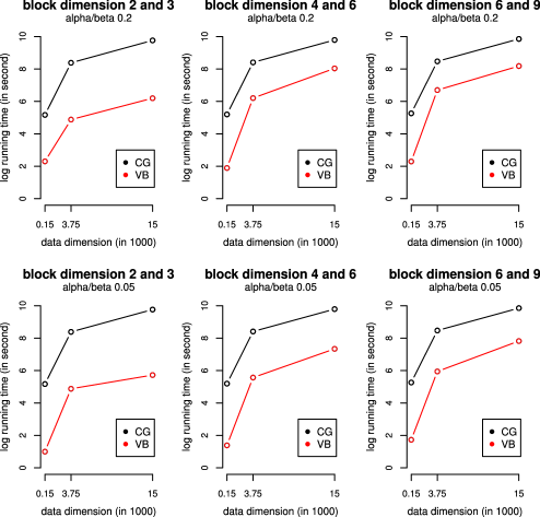
Figure 1: Log run-time for simulated data. Red lines represent variational Bayes and black lines represent MCMC via collapsed Gibbs. The $x$-axis is the number of elements in a table. For instance, 0.15 (thousand) represents a 10 by 15 table with 150 elements.

Table 5: Comparison of vEM fits using informative and noninformative priors, in terms of estimation error $\varepsilon_{B}$ and accuracy in estimating the highest membership component

Noninformative priors			Informative priors
$\bolds{\varepsilon_{B}}$	Row	Column	$\bolds{\varepsilon_{B}}$	Row	Column
0.385 (0.176)	0.868 (0.121)	0.827 (0.134)	0.203 (0.121)	0.788 (0.157)	0.870 (0.091)

3.6 Run-time comparison

As seen previously, variational Bayes performs as effectively as MCMC in parameter and membership estimation as well as held-out prediction accuracy. In the following, we present results on run-time comparison between these two approaches. Our goal is to quantify the magnitude of savings that variational Bayes can achieve while obtaining similar inferences to those obtained through MCMC.

For each experiment we run 10 times, and the average log run-time is recorded. The plots are shown in Figure 1. Three table sizes are considered in this simulation: $10\times 15$, $50\times 75$ and $100\times 150$. From this figure, the run-time for MCMC is consistently several times larger more than that of variational Bayes. For example, when block sizes equal $(6,9)$, and Dirichlet parameters equal 0.05, one experiment takes about 30 minutes to run for variational Bayes, and it takes roughly 6 hours for MCMC. This trend continues when table size increases, and the saving on computational cost can be much more. These results suggest that variational Bayes should be preferred for analyzing large tables. Recently developed inference strategies based on spectral clustering [Rohe and Yu (2012)] and binary factor graphs [Azari and Airoldi (2012)] should also be considered.

3.7 Quantifying the effects of censoring

One of the issues in existing studies of coordinated cellular responses is the preprocessing of the original measurements. This kind of censoring reduces data utility and decreases estimation accuracy. The goal of this study is to quantify the effects of censoring by thresholding on the estimation of the blockmodel.

The data $Y$ are generated from $Y(j,k)\sim\operatorname{Normal}(\vec{\pi}_{j}^{\prime}B\vec{p_{k}},\sigma^{2})$. The domain of $Y(j,k)$ is $(-\infty,+\infty)$. We perform Inverse Fisher Transformation (IFT) that maps $Y(j,k)$ to $\rho(j,k)$ so that its range is $[-1,1]$. The censored data are defined as $S(j,k)=\mathbf{1}(|\rho(j,k)|\geq\tau)$, where $\tau$ can be median, mean or 0.5. Clearly, $S(j,k)\in\{0,1\}$.

The Normal blockmodel is applied to the original data $Y(j,k)$ and the Bernoulli blockmodel described in Section 2.2 is applied to the censored data $S(j,k)$. To make the comparison in the same scale, we define $\hat{\rho}(j,k)$ as the IFT of $\vec{\phi}_{j\rightarrow k}^{\prime}\hat{B}\vec{\eta}_{j\leftarrow k}$, where $\vec{\phi}_{j\rightarrow k}$, $\hat{B}$ and $\vec{\eta}_{j\leftarrow k}$ are estimated from the Normal blockmodel. The estimation error is defined as

$$\varepsilon=\frac{\sum_{(j,k)}|\rho(j,k)-\hat{\rho}{(j,k)}|}{N_{1}\times N_{2}}.$$

The estimation error for the censored experiment is computed in the same fashion, with $\hat{\rho}(j,k)=\vec{\phi}_{j\rightarrow k}^{\prime}\hat{B}\vec{\eta}_{j\leftarrow k}$, where $\vec{\phi}_{j\rightarrow k}$, $\hat{B}$ and $\vec{\eta}_{j\leftarrow k}$ are estimated from the Bernoulli blockmodel, and $\rho(j,k)$ replaced by $|\rho(j,k)|$.

Table 6: Comparison of estimation error on censored and noncensored data. Standard errors are inside the parenthesis

Data	Method	Bic.	Error $\bolds{\varepsilon}$	Recall	Precision
Raw $\rho_{ij}$	2-way Normal	6	$0.054\mbox{ }(0.010)$	$0.841\mbox{ }(0.169)$	$0.881\mbox{ }(0.116)$
	Hier. clustering	6	$0.221\mbox{ (--)}$	$0.967\mbox{ (--)}$	$0.970\mbox{ (--)}$
	Cheng & Church	2	–	$0.367\mbox{ (--)}$	$0.679\mbox{ (--)}$
$|\rho_{ij}|>\rho_{(0.5)}$	2-way Bernoulli	6	$0.175\mbox{ }(0.006)$	$0.518\mbox{ }(0.017)$	$0.722\mbox{ }(0.048)$
	Hier. clustering	6	$0.125\mbox{ (--)}$	$0.700\mbox{ (--)}$	$0.850\mbox{ (--)}$
	Cheng & Church	2	–	$0.232\mbox{ (--)}$	$0.640\mbox{ (--)}$
	Cross-associations	4	–	$0.667\mbox{ (--)}$	$0.762\mbox{ (--)}$
$|\rho_{ij}|>\bar{\rho}$	2-way Bernoulli	6	$0.182\mbox{ }(0.003)$	$0.528\mbox{ }(0.014)$	$0.773\mbox{ }(0.056)$
	Hier. clustering	6	$0.187\mbox{ (--)}$	$0.500\mbox{ (--)}$	$0.841\mbox{ (--)}$
	Cheng & Church	3	–	$0.237\mbox{ (--)}$	$0.640\mbox{ (--)}$
	Cross-associations	6	–	$0.667\mbox{ (--)}$	$0.841\mbox{ (--)}$
$|\rho_{ij}|>0.5$	2-way Bernoulli	6	$0.158\mbox{ }(0.002)$	$0.528\mbox{ }(0.022)$	$0.835\mbox{ }(0.030)$
	Hier. clustering	6	$0.189\mbox{ (--)}$	$0.500\mbox{ (--)}$	$0.841\mbox{ (--)}$
	Cheng & Church	3	–	$0.239\mbox{ (--)}$	$0.640\mbox{ (--)}$
	Cross-associations	8	–	$0.613\mbox{ (--)}$	$0.667\mbox{ (--)}$

We compare our model with a bi-clustering method popular in computational biology [Cheng and Church (2000)], fit to both the raw and censored correlations. We match each estimated bicluster to a true block and compute recall and precision in estimating absolute correlations above a threshold. Results are presented in Table 6, where the results obtained with BCCC are optimized over a range of input parameter values. For completeness, we also add results obtained with hierarchical clustering to rows and columns independently, and with cross-association [Chakrabarti et al. (2004)].

The effects of censoring are clearly seen from Table 6. The estimation error increases more than threefold when using the censored data with the Bernoulli block model. The effect of thresholding parameter $\tau$ is not very significant.

4 Analyzing transcriptional and metabolic coordination in response to starvation

Functions in a cell are executed by cascades of molecular events. Intuitively, proteins are the messengers, while metabolites and other small molecules are the messages. Measuring protein activity over time, directly, is difficult and expensive. An indication of the abundance of most proteins, however, can be inferred from the amount of the messenger RNA transcripts. These transcripts are copies of genes and lead to the translation of proteins. This is especially true in yeast where alternatives to the transcription-translation hypothesis, such as alternative splicing, are not frequent. Metabolite concentrations add an essential perspective to the study of cascades of molecular events.

We conducted an integrated analysis of two data collections recently published: temporal profiles of metabolite concentrations [Brauer et al. (2006)] and temporal profiles of gene expression [Bradley et al. (2009)], both measured in Saccharomyces cerevisiae with matching sampling schemes.

An integrated analysis of the coordination between gene expression and metabolite concentrations may lead to the identification of sets of genes (i.e., the corresponding proteins) and metabolites that are functionally related, which will provide additional insights into regulatory mechanisms at multiple levels and open avenues of inquiry. The identification and quantification of such coordinated regulatory behavior is the goal of our analysis.

The methodology in Section 2 allows us to identify genes and metabolites that show correlated responses to metabolic stress, namely, starvation. To evaluate the biological significance of the results, we quantify to what extent correlated responses are associated with metabolic-related functions and to what extent estimated models can be used to identify functionally related genes and metabolites out-of-sample.

4.1 Data and experimental design

The expression data consist of messenger RNA transcript levels measured using Agilent microarrays on cultures of S. cerevisiae before and after carbon starvation (glucose removal), and before and after nitrogen starvation (ammonium removal). Collection times were 0 minutes (before starvation) and 10, 30, 60, 120, 240 and 480 minutes after starvation. For more details about the data and the experimental protocol see Bradley et al. (2009). The metabolite concentrations data were obtained using liquid chromatography-mass spectrometry before and after carbon starvation (glucose removal), and before and after nitrogen starvation (ammonium removal). Collection times were 0 minutes (before starvation) and 10, 30, 60, 120, 240 and 480 minutes after starvation. For more details about the data and the experimental protocol see Brauer et al. (2006).

The concentration of each metabolite and the transcript level of each gene at time point $t$ are expressed as $\log_{2}$ ratios versus the corresponding measurements at the zero time point. Thus, for each gene $j$ we have a sequence $G_{jt}$, $t=1,\ldots,6$, and for each metabolite $k$ we have a sequence $M_{kt}$, $t=1,\ldots,6$, representing for the 6 time points observation after time 0. Complete temporal profiles are available for 5039 genes and for 61 metabolites; 783 genes and 7 metabolites with missing data were not considered.

Using the temporal profile, we can calculate the sample correlation coefficient of each gene and metabolite pair $(j,k)$: $\rho(j,k)=\frac{\sum_{t=1}^{T}(G_{jt}-\bar{G}_{j})(M_{kt}-\bar{M}_{k})}{(T-1)S_{G}S_{M}}$, where $\bar{G}_{j}=\sum_{t}G_{jt}/T$ and $\bar{M}_{k}=\sum_{t}M_{kt}/T$ are the sample mean, and $S_{G}$ and $S_{M}$ are the sample standard deviation. We then transform these correlations using the Fisher transformation $Z(j,k)=\frac{1}{2}\log\frac{1+\rho{(j,k)}}{1-\rho{(j,k)}}$. With the true correlation between genes and metabolites denoted as $\rho_{0}$, we have $Z(j,k)$ following asymptotically Normal distribution with mean $\mu_{z}=\frac{1}{2}\log\frac{1+\rho_{0}}{1-\rho_{0}}$ and standard error $1/\sqrt{T-3}$ [Fisher (1915, 1921)]. Under the hypothesis that there is no correlation between genes and metabolites, we will expect $\rho_{0}=0$ and $\mu_{z}=\frac{1}{2}\log\frac{1+\rho_{0}}{1-\rho_{0}}=0$. These Fisher transformed quantities provide the input to our model.

We do not expect the multi-way blockmodel assumption to hold for all the 5039 genes. Instead, we provide separate joint analyses on subsets of genes and all 61 metabolites, for a number of gene lists of interest, which we expect to be involved in the cellular response to starvation. We consider gene lists that were obtained in studies exploring the environmental stress response (ESR), cellular proliferation, metabolism and the cell cycle [Gasch et al. (2000), Tu et al. (2005), Brauer et al. (2008), Airoldi et al. (2009, 2013a), Slavov et al. (2013)].

For all the experiments we rely on variational Bayes implementation of our model due to its advantage in convergence speed, which is crucial when dealing with correlation tables involving hundreds of genes. We adopt the setting as described in Section 3.6 for VB, with specific changes described as they become relevant. In the remainder of this section, with the exception of Section 4.5, we consistently set the number of metabolite blocks $K_{2}=4$, since there are four metabolite classes, and we use informative priors for the memberships of each metabolite, depending on which class they are known to belong to. Specifically, each of the 61 metabolites belongs to one of the four classes: TCA, AA, GLY, BSI. If a metabolite is in class TCA, say, Aconitate, its $\vec{\xi}$ vector will be initialized as $\vec{\xi}={}$[100 1 1 1], normalized to unit norm. By assuming a dominating component on the true index in the initial membership, the metabolites will mostly remain stably associated to their classes during VB inference.

For the optimal number of gene blocks, we select $K_{1}$ by minimizing the Bayesian information criterion (BIC). The general BIC formula is $-2\log L+k\times\log(n)$, in which $k$ is the number of parameters, $n$ is the number of observations, and $L$ is the likelihood. For our model, the approximated BIC is

$$-2\log L+|B,\vec{\pi},\vec{p}|\times\log|Y|,$$

where $|B,\vec{\pi},\vec{p}|$ is the number of parameters, which is approximately equal to $K_{1}\times K_{2}$, and $|Y|$ is the number of entries in the table, that is, $|Y|=N_{1}\times N_{2}$.

In Section 4 we present some of the results with the goal of showcasing how the data analysis, via the multi-way block model, supports the biological research.

4.2 Multifaceted functional evaluation of coordinated responses

Here we evaluate to what extent the proposed model is useful in revealing the genes’ multifaceted functional roles. We rely on the functional enrichment analysis using the Gene Ontology to evaluate the functional content of clusters of genes [Ashburner et al. (2000), Boyle et al. (2004)].

Table 7: Example functional evaluation. Gene Ontology terms associated with first- and second-largest membership scores for the Nitrogen starvation experiment

Memb.	Class	Ontology	Term description	$\bolds{p}$-value
First	AA	Component	DNA-directed RNA polymerase I complex	$9.8\mbox{E--}6$
First	AA	Component	Preribosome, small subunit precursor	$0.00324$
First	AA	Function	Translation factor activity, nucleic acid binding	$5.11\mbox{E--}14$
First	AA	Function	Translation initiation factor activity	$1.64\mbox{E--}10$
First	AA	Function	DNA-directed RNA polymerase activity	$1.45\mbox{E--}6$
First	BSI	Component	Preribosome, large subunit precursor	$0.00013$
First	BSI	Function	GTP binding	$0.03314$
First	BSI	Function	Guanyl ribonucleotide binding	$0.03314$
Second	AA	Component	DNA-directed RNA polymerase III complex	$6.76\mbox{E--}10$
Second	AA	Component	DNA-directed RNA polymerase II core complex	$0.00322$
Second	AA	Function	RNA polymerase activity	$1.27\mbox{E--}6$
Second	AA	Function	ATP-dependent RNA helicase activity	$3.43\mbox{E--}6$
Second	BSI	Component	Ribonucleoprotein complex	$6.47\mbox{E--}12$
Second	BSI	Component	90S preribosome	$0.00124$
Second	BSI	Function	Aminoacyl-tRNA ligase activity	$0.0000817$
Second	BSI	Function	N-methyltransferase activity	$0.0455$

One aspect of our model that distinguishes it from clustering and bi-clustering methods is the mixed membership assumption. That is, in our model, each gene can participate in multiple functions, as modeled via the gene-specific latent membership vectors $\vec{\pi}$. In practice, the membership assumption lets us identify multiple levels of functional enrichment.

To illustrate this point, we consider 521 genes that were found to be strongly associated with metabolic activities, that is, up-regulated in response to increasing growth rate, in previous studies [Brauer et al. (2008), Airoldi et al. (2009)]. We use the largest estimated memberships for each gene $\pi_{gi}$, $i=1,\ldots,K_{1}$, to assign genes $g=1,\ldots,521$ to metabolite classes $j=1,\ldots,4$. Then we perform functional analysis on the resulting sets of genes associated with each metabolite class.

More formally, we proceed as follows. First, the largest estimated membership is used to assign gene $g$ to gene block $i$, according to $\hat{i}_{g}=\break\arg\max_{i=1,\ldots,K_{1}}\pi_{gi}$. Then the largest estimated gene-block to metabolite-class association $|B_{ij}|$ is then used to assign gene $g$ with a metabolite class, according to

$$\hat{j}_{g}=\mathop{\arg\max}_{j=1,\ldots,4}|B_{\hat{i}_{g},j}|.$$

The collection of estimated gene-to-metabolite class associations, $\{\hat{j}_{g}$, $g=1,\ldots,521\}$, is used to partition genes into four sets, for example, $AA=\{g\mbox{ s.t. }\hat{j}_{g}=1\}$. We perform functional enrichment analysis for each of these four sets. In addition, the mixed membership nature of the proposed multi-way blockmodel allows us to analyze second-order functional enrichment. We repeat the procedure above but we estimate $\hat{i}_{g}$ using the second-largest membership in $\vec{\pi}_{g}$.

The functional analysis results obtained for both first- and second-largest memberships are reported in Table 7. Interestingly, subsets of genes associated with the same metabolite class, for instance, AA, are functionally enriched for multiple functions, to different degrees. For instance, genes use AA metabolites when performing translational activities in the nucleus primarily, however, they use AA metabolites when performing polymerase-related activities on the polymerase II and II complexes to a lesser extent. Similarly, genes use BSI metabolites for binding activities in the preribosome primarily, and for ligase and transferase activities in the preribosome and the ribonucleoprotein complex to a minor extent. The magnitude of the components of the relevant mixed membership vectors provides more information on the degree of involvement the various gene blocks in these many activities. This type of multifaceted functional analysis is possible thanks to the mixed membership assumption encoded in the multi-way blockmodel.

These results highlight the role of the mixed membership assumption in supporting a detailed multifaceted functional analysis, which is not possible with traditional methods.

4.3 Predicting functional annotations out-of-sample

Here we assess the goodness of fit of the proposed method on real data, in terms of predictions out-of-sample. We present results of an experiment in which we predict held-out functional annotations $\pi_{gi}$. This analysis leverages use of informative priors on a subset of known functional annotations.

We consider 57 genes that were found in previous studies to be strongly associated with cellular growth [Brauer et al. (2008), Airoldi et al. (2009)], 760 genes that were found to be involved in the environmental response to stress [Gasch et al. (2000)], and 19 genes that were found to be involved in metabolic cycling [Tu et al. (2005)].

Good out-of-sample prediction performance will enable biologists to use this method to guide which functions they should be testing at the bench, speeding up the exploration of the functional landscape through statistical analysis of gene–metabolite associations.

Table 8: Statistics for the lists of genes. Column three reports the number of genes with one, some and no functional annotations. $K_{1}$ is the number of gene blocks in the fitted blockmodel

	No. of genes		No. of functional annotations
Gene list	Total	One/some/none	Min	25%	50%	75%	Max	Mean	$\bolds{K_{1}}$
Growth rate	$57$	$5/19/38$	1	$1.25$	$4$	$7$	$7$	$\phantom{0}4.26$	12
ESR induced	$240$	$0/215/25$	2	$5$	$7$	$12$	$31$	$9.31$	76
ESR repressed	$520$	$1/503/17$	1	$10$	$19$	$22$	$31$	$16.93$	78
Metabolic cycle	$19$	$4/14/5$	1	$1$	$6.5$	$10$	$20$	$7.29$	25

To establish the ground truth for this experiment, we collected functional annotations for each gene in the same four lists as in Section 4.2 which will be held-out and predicted using the multi-way blockmodel. Table 8 reports summary statistics of the functional annotations in each list of genes, obtained using the Gene Ontology term finder (SGD). Column two reports the total number of genes in each list. Column three reports the number of genes with one, some and no functional annotations. Columns 4–9 report the quantiles from the distribution of the number of functional annotations for the genes in each list. Column 10 reports the value of $K_{1}$ we selected for fitting the blockmodel.

Table 9: Out-of-sample predictions of functional annotations for the Nitrogen starvation experiment. Accuracy in recovering (single/multiple) annotations for four lists of genes

	Single annotations				Multiple annotations
	Observed		Missing		Observed		Missing
Gene list	0s	1s	0s	1s	0s	1s	0s	1s
Growth rate	0.94	0.36	0.94	0.36	0.83	0.75	0.84	0.74
ESR induced	–	–	–	–	0.92	0.39	0.92	0.46
ESR repressed	–	–	0.99	0.00	0.84	0.43	0.85	0.50
Metabolic cycle	0.97	0.25	0.96	0.10	0.78	0.65	0.80	0.63

To perform the second experiment, we held out the annotations for 50% of the genes with multiple functional annotations, and we also held out the annotation for 50% of the genes with a single functional annotation. When fitting the multi-way blockmodel, in addition to using informative priors for the memberships of each metabolite depending on which class they are known to belong, as detailed in Section 4.1, we used informative priors for the functional annotations we did not hold out. For the held-out annotations, we used noninformative values for the hyperparameters instead. For instance, suppose that the known vector of functional annotations for gene $g$ is $\vec{a}_{g}={}$[1 0 0 1 1 0 0 0 0 1], and that $a_{g}(1)$ and $a_{g}(4)$ were to be held out in a particular replication, so that we have $\vec{a}_{g}={}$[NA 0 0 NA 1 0 0 0 0 1]. The prior for the functional annotation for that gene would be set at $\vec{\xi}_{g}={}$[1 1 1 1 100 1 1 1 1 100], normalized to unit norm. The rationale for this choice is to fit a multi-way blockmodel with known biological structure for those genes and metabolites that are used for parameter estimation, but agnostic about the biology we want to predict out-of-sample. We claimed success in each prediction if the imputed annotations, $\hat{\xi}_{g}(k)=1$, corresponded to real held-out annotations, and if the imputed absences of annotations, $\hat{\xi}_{g}(i)=0$, corresponded to absences of real held-out annotations. We repeated this procedure 10 times, for each of the four lists of genes.

Table 9 reports the accuracy results, detailed by genes with single and multiple annotations, and evaluated separately for annotations (i.e., the 1s) and lack of annotations (i.e., the 0s). The baseline accuracy for predicting single annotations, using random guesses for each gene independently, ranges between $1/19\approx 5\%$ for the metabolic cycle genes to $1/520\approx 0.2\%$ for the ERS genes. The baseline accuracy is slightly higher for predicting multiple annotations, since predicting single annotations is a harder problem.

For completeness, we also report the accuracy in predicting annotations that were known during model fitting to get a sense of the goodness of fit from a substantive, biological perspective. In fact, if the model assumptions are accurate, we would expect accurate predictions for the known annotations. If the model is not accurate, or if the model provides too much shrinkage, we would expect lower accuracy on known annotations.

Overall, the blockmodel assumptions are substantiated by the results in Table 9. The model is useful for encoding biological information about single and multiple functional annotations. The out-of-sample prediction accuracy of the multi-way blockmodel is solid and consistently much higher than the baseline. These results complement and confirm the out-of-sample prediction results we obtained in Section 3.3.

4.4 Coordinated and differential regulatory response to Nitrogen and Carbon starvation

Here we provide an illustration of how the multi-way blockmodel can be used to perform quantitative and qualitative analysis of coordinated regulation in response to Nitrogen starvation and differential regulation in response to Carbon starvation. We perform this analysis for the same four lists of genes we considered in Section 4.2.

Table 10: Quantitative evaluation of coordinated regulatory responses. Number of genes associated with the same metabolite class in both the Nitrogen and Carbon starvation experiments. The association is estimated using both largest and second-largest membership scores

	Largest membership				Second-largest membership
Gene list	AA	BSI	GLY	TCA	AA	BSI	GLY	TCA
Growth rate	$11$	$6$	$10$	$2$	$10$	$5$	3	$1$
ESR induced	$55$	$13$	$4$	$0$	$48$	$21$	4	$0$
ESR repressed	$128$	$22$	$1$	$17$	$109$	$52$	0	$27$
Metabolic cycle	$2$	$3$	$1$	$0$	$2$	$3$	1	$0$

The quantitative analysis of coordinated regulation is based on the number of genes which are estimated to be associated with the various metabolite classes, in both the Nitrogen and the Carbon starvation experiments.

We used the same procedure described in Section 4.2 to estimate the metabolite classes associated with each gene, using the estimated largest and second-largest (gene-block) memberships. Table 10 reports the number of genes that were found to be associated with a primary metabolite class (largest membership) and with a secondary metabolite class (second-largest membership) for each of the four lists of genes we consider.

About a fourth of the genes are found to be associated with a primary metabolite class. Despite the similarity in the patterns of primary and secondary associations, the gene sets involved in them are different. These results imply that another fourth of the genes are found to be associated to a secondary metabolite class. Overall, the blockmodel suggests a substantial amount of overlap between the coordinated regulatory response to Nitrogen and Carbon starvation. A similar quantitative analysis could be conducted for highlighting Nitrogen- and Carbon-specific coordinated regulatory responses.

Table 11: Functional evaluation of gene–metabolite associations that are differentially regulated in Nitrogen and Carbon. Gene Ontology terms for gene–metabolite associations unique to the Nitrogen starvation experiment. Association is computed using the largest memberships

Class	Ontology	Term description	$\bolds{p}$-value
AA	Function	Alcohol dehydrogenase (NADP$+$) activity	$0.01775$
AA	Function	Aldo-keto reductase (NADP) activity	$0.01775$
AA	Process	Vacuolar protein catabolic process	$0.00026$
AA	Process	Catabolic process	$0.00808$
BSI	Function	Peroxidase activity	$0.0000568$
BSI	Function	Antioxidant activity	$0.0004$
BSI	Function	Carbohydrate kinase activity	$0.00083$
BSI	Function	Glutathione peroxidase activity	$0.0214$
BSI	Process	Carbohydrate catabolic process	$2.98\mbox{E--}7$
BSI	Process	Cellular response to oxidative stress	$0.0000131$
BSI	Process	Trehalose metabolic process	$0.0000203$
BSI	Process	Alcohol catabolic process	$0.0000231$
BSI	Process	Glycoside metabolic process	$0.000061$
GLY	Function	Oxidoreductase activity	$0.0000116$
GLY	Process	Oxidation–reduction process	$0.00097$
GLY	Process	Cellular carbohydrate metabolic process	$0.0011$
GLY	Process	Carbohydrate metabolic process	$0.00143$
GLY	Process	Cellular aldehyde metabolic process	$0.00351$

The qualitative analysis of differential regulation is based on the functional enrichment analysis of those genes associated with a given metabolite class in the Nitrogen experiment, but associated with a different metabolic class in the Carbon experiment. For this analysis, we used the procedure above to estimate the metabolite classes associated with each gene, using the estimated largest memberships only, for the list of genes that were found to be ESR induced. The results of the functional analysis obtained for the largest memberships, using the Gene Ontology term finder, are reported in Table 11.

These results highlight how the same set of genes (a proxy for proteins) may be using metabolites differently to execute a response to the Carbon. For instance, metabolites in the BSI class are used to process glycoside, alcohol and trehalose, as part of antioxidant activities. Metabolites in the GLY class are used to execute oxidoreductase activities and metabolize aldehyde and carbohydrates. The magnitude of the components of the relevant mixed membership vectors provides more information on the degree of involvement the various gene blocks in these many activities.

A similar qualitative analysis could be carried out to explore the functional landscape, that is, shared by the Nitrogen and Carbon coordinated regulatory responses to starvation.

4.5 Comparative analysis of raw and preprocessed data

Here we compare a blockmodel analysis of coordinated regulation with an analysis using cross-association Chakrabarti et al. (2004), quantitatively, in terms of number of gene–metabolite class associations found. We consider the four lists of genes above for this analysis.

Cross-association takes a binary table as input. We built such a genes-by-metabolites binary matrix $Y$ by thresholding the corresponding matrix of correlations. We assign $Y(j,k)=1$ whenever $\rho(j,k)$ is above the 75th percentile or below the 25th percentile of the empirical correlation distribution.

Cross-association provides a two-way blockmodel as output, in which $K_{1}$ and $K_{2}$ are estimated using a metric based on information gain. To make a valid comparison, we fit the stochastic multi-way blockmodel with the same number of gene and metabolite blocks.

An additional complication in this analysis is that the number of metabolite blocks can be different from four, for both cross-association and the stochastic blockmodel. We use noninformative priors on the metabolites memberships in the stochastic blockmodel. In addition, we developed a greedy matching procedure to associate metabolite blocks to metabolite classes, after inference. We proceeded as follows. Each metabolite was associated with a block using its largest (metabolite-block) membership. Each metabolite is associated with a known metabolite class. We assigned a metabolite class label to each metabolite block according to a simple majority rule.

We used the same procedure described in Section 4.2 to estimate the metabolite classes associated with each gene, using the estimated largest and second-largest (gene-block) memberships.

Table 12 reports the number of Gene Ontology terms that were found to be associated with a primary metabolite class (largest membership) in the first four rows, and with a secondary metabolite class (second-largest membership) in the next four rows, for each of the four lists of Gene Ontology terms we consider. The last four rows report the number of genes that were found to be associated with a metabolite class using cross-association. The multi-way stochastic blockmodel finds more primary associations than cross-association, 246 versus 194. In addition, if we consider the secondary associations, the blockmodel analysis uncovers 190 more associations. In fact, subsets of genes associated with the same primary and secondary metabolite class, for instance, AA, are not overlapping by construction.

Table 12: Quantitative evaluation of Gene Ontology terms associated with gene–metabolite class found. Shown in the tables are results for multi-way blockmodel’s largest (1st) and second-largest (2nd) memberships as well as cross-associations (CA)

		AA			BSI			TCA
Memb.	Gene list	BP	CC	MF	BP	CC	MF	BP	CC	MF	Total
1st	Growth rate	$1$	–	–	$1$	$6$	$5$	–	–	–	$13$
1st	ESR induced	$33$	$7$	$11$	$2$	$1$	$2$	16	–	5	$77$
1st	ESR repressed	–	$45$	$26$	$32$	$23$	$5$	–	–	–	$131$
1st	Metabolic cycle	$13$	$6$	$6$	–	–	–	–	–	–	$25$
2nd	Growth rate	$4$	$6$	$3$	–	–	–	–	–	–	$13$
2nd	ESR induced	–	$1$	$6$	–	$16$	$14$	–	–	1	$38$
2nd	ESR repressed	–	$47$	$21$	–	$34$	$11$	–	–	–	$113$
2nd	Metabolic cycle	–	–	–	$12$	$6$	$8$	–	–	–	$26$
CA	Growth rate	–	$6$	$2$	$2$	–	$2$	–	–	–	$12$
CA	ESR induced	–	–	–	–	$21$	$19$	–	–	–	$40$
CA	ESR repressed	–	$47$	$20$	–	$30$	$20$	–	–	–	$117$
CA	Metabolic cycle	–	–	–	$12$	$6$	$7$	–	–	–	$25$

Overall, cross-association is not well suited for any analysis of biological correlations because of a number of shortcomings, including its reliance on binary input and its lack of flexibility for incorporating prior biological information, for example, the number of metabolite blocks. Our results show that the multi-way stochastic blockmodel outperforms cross-associations quantitatively, even when we do not make use of biological prior knowledge.

5 Concluding remarks

In order to analyze the temporal coordination between gene expression and metabolite concentrations in yeast cells, in response to starvation, we developed a family of multi-way stochastic blockmodels. These models extend the mixed membership stochastic blockmodel [Airoldi et al. (2008)] to the case of two sets of measurements and to the case of Gaussian and binary responses. We developed and compared various inference schemes for multi-way blockmodels, including Monte Carlo Markov chains and variational Bayes.

We further explored the impact of thresholding and binning on the analysis. These censoring mechanisms are often used as preprocessing steps. The transformed data are then amenable to the analysis of coordination using off-the-shelf methods, including Bayesian networks and popular blocking algorithms from the data mining literature [Bradley et al. (2009), Chakrabarti et al. (2004)]. The sensitivity analysis suggests that the impact of preprocessing steps that involve censoring is substantial, both from a quantitative perspective and in terms of its impact on biological discovery, in our case study.

References

- Airoldi (2007) {barticle}[auto:STB—2013/10/14—10:36:11] \bauthor\bsnmAiroldi, \bfnmE. M.\binitsE. M. (\byear2007). \btitleGetting started in probabilistic graphical models. \bjournalPLoS Computational Biology \bvolume3 \bpagese252. \bptokimsref \endbibitem
- Airoldi et al. (2008) {barticle}[auto:STB—2013/10/14—10:36:11] \bauthor\bsnmAiroldi, \bfnmE. M.\binitsE. M., \bauthor\bsnmBlei, \bfnmD. M.\binitsD. M., \bauthor\bsnmFienberg, \bfnmS. E.\binitsS. E. and \bauthor\bsnmXing, \bfnmE. P.\binitsE. P. (\byear2008). \btitleMixed membership stochastic blockmodels. \bjournalJournal of Machine Learning Research \bvolume9 \bpages1981–2014. \bptokimsref \endbibitem
- Airoldi et al. (2009) {barticle}[auto:STB—2013/10/14—10:36:11] \bauthor\bsnmAiroldi, \bfnmE. M.\binitsE. M., \bauthor\bsnmHuttenhower, \bfnmC.\binitsC., \bauthor\bsnmGresham, \bfnmD.\binitsD., \bauthor\bsnmLu, \bfnmC.\binitsC., \bauthor\bsnmCaudy, \bfnmA.\binitsA., \bauthor\bsnmDunham, \bfnmM.\binitsM., \bauthor\bsnmBroach, \bfnmJ. R.\binitsJ. R., \bauthor\bsnmBotstein, \bfnmD.\binitsD. and \bauthor\bsnmTroyanskaya, \bfnmO. G.\binitsO. G. (\byear2009). \btitlePredicting cellular growth from gene expression signatures. \bjournalPLoS Computational Biology \bvolume5 \bpagese1000257. \bptokimsref \endbibitem
- Airoldi et al. (2013a) {bmisc}[auto:STB—2013/10/14—10:36:11] \bauthor\bsnmAiroldi, \bfnmE. M.\binitsE. M., \bauthor\bsnmHashimoto, \bfnmT. B.\binitsT. B., \bauthor\bsnmBrandt, \bfnmN.\binitsN., \bauthor\bsnmBahmani, \bfnmT.\binitsT., \bauthor\bsnmAthanasiadou, \bfnmN.\binitsN. and \bauthor\bsnmGresham, \bfnmD. J.\binitsD. J. (\byear2013a). \bhowpublishedCoordinated dynamics of cell growth and transcription. Preprint. \bptokimsref \endbibitem
- Airoldi, Wang and Lin (2013b) {bmisc}[auto:STB—2013/10/14—10:36:11] \bauthor\bsnmAiroldi, \bfnmE. M.\binitsE. M., \bauthor\bsnmWang, \bfnmX.\binitsX. and \bauthor\bsnmLin, \bfnmX.\binitsX. (\byear2013b). \bhowpublishedSupplement to “Multi-way blockmodels for analyzing coordinated high-dimensional responses.” DOI:\doiurl10.1214/13-AOAS643SUPP. \bptokimsref \endbibitem
- Ashburner et al. (2000) {barticle}[auto:STB—2013/10/14—10:36:11] \bauthor\bsnmAshburner, \bfnmM.\binitsM., \bauthor\bsnmBall, \bfnmC. A.\binitsC. A., \bauthor\bsnmBlake, \bfnmJ. A.\binitsJ. A., \bauthor\bsnmBotstein, \bfnmD.\binitsD., \bauthor\bsnmButler, \bfnmH.\binitsH., \bauthor\bsnmCherry, \bfnmJ. M.\binitsJ. M., \bauthor\bsnmDavis, \bfnmA. P.\binitsA. P., \bauthor\bsnmDolinski, \bfnmK.\binitsK., \bauthor\bsnmDwight, \bfnmS. S.\binitsS. S., \bauthor\bsnmEppig, \bfnmJ. T.\binitsJ. T., \bauthor\bsnmHarris, \bfnmM. A.\binitsM. A., \bauthor\bsnmHill, \bfnmD. P.\binitsD. P., \bauthor\bsnmIssel-Tarver, \bfnmL.\binitsL., \bauthor\bsnmKasarskis, \bfnmA.\binitsA., \bauthor\bsnmLewis, \bfnmS.\binitsS., \bauthor\bsnmMatese, \bfnmJ. C.\binitsJ. C., \bauthor\bsnmRichardson, \bfnmJ. E.\binitsJ. E., \bauthor\bsnmRingwald, \bfnmM.\binitsM., \bauthor\bsnmRubinand, \bfnmG. M.\binitsG. M. and \bauthor\bsnmSherlock, \bfnmG.\binitsG. (\byear2000). \btitleGene ontology: Tool for the unification of biology. The gene ontology consortium. \bjournalNature Genetics \bvolume25 \bpages25–29. \bptokimsref \endbibitem
- Azari and Airoldi (2012) {barticle}[auto:STB—2013/10/14—10:36:11] \bauthor\bsnmAzari, \bfnmH.\binitsH. and \bauthor\bsnmAiroldi, \bfnmE. M.\binitsE. M. (\byear2012). \btitleGraphlet decomposition of a weighted network. \bjournalJournal of Machine Learning Research, W&CP (AI&Stat) \bvolume22 \bpages54–63. \bptokimsref \endbibitem
- Blei and Jordan (2006) {barticle}[mr] \bauthor\bsnmBlei, \bfnmDavid M.\binitsD. M. and \bauthor\bsnmJordan, \bfnmMichael I.\binitsM. I. (\byear2006). \btitleVariational inference for Dirichlet process mixtures. \bjournalBayesian Anal. \bvolume1 \bpages121–143 (electronic). \biddoi=10.1214/06-BA104, mr=2227367 \bptokimsref \endbibitem
- Blocker and Meng (2013) {barticle}[auto:STB—2013/10/14—10:36:11] \bauthor\bsnmBlocker, \bfnmA. W.\binitsA. W. and \bauthor\bsnmMeng, \bfnmX. L.\binitsX. L. (\byear2013). \btitleThe perils of data pre-processing. \bjournalBernoulli \bvolume19 \bpages1176–1211. \bptokimsref \endbibitem
- Boyle et al. (2004) {barticle}[auto:STB—2013/10/14—10:36:11] \bauthor\bsnmBoyle, \bfnmE. I.\binitsE. I., \bauthor\bsnmWeng, \bfnmS.\binitsS., \bauthor\bsnmGollub, \bfnmJ.\binitsJ., \bauthor\bsnmJin, \bfnmH.\binitsH., \bauthor\bsnmBotstein, \bfnmD.\binitsD., \bauthor\bsnmCherry, \bfnmJ. M.\binitsJ. M. and \bauthor\bsnmSherlock, \bfnmG.\binitsG. (\byear2004). \btitleGO::TermFinder—open source software for accessing gene ontology terms associated with a list of genes. \bjournalBioinformatics \bvolume20 \bpages3710–3715. \bptokimsref \endbibitem
- Bradley et al. (2009) {barticle}[auto:STB—2013/10/14—10:36:11] \bauthor\bsnmBradley, \bfnmP. H.\binitsP. H., \bauthor\bsnmBrauer, \bfnmM. J.\binitsM. J., \bauthor\bsnmRabinowitz, \bfnmJ. D.\binitsJ. D. and \bauthor\bsnmTroyanskaya, \bfnmO. G.\binitsO. G. (\byear2009). \btitleCoordinated concentration changes of transcripts and metabolites in Saccharomyces cerevisiae. \bjournalPLoS Computational Biology \bvolume5 \bpagese1000270. \bptokimsref \endbibitem
- Brauer et al. (2008) {barticle}[auto:STB—2013/10/14—10:36:11] \bauthor\bsnmBrauer, \bfnmM. J.\binitsM. J., \bauthor\bsnmHuttenhower, \bfnmC.\binitsC., \bauthor\bsnmAiroldi, \bfnmE. M.\binitsE. M., \bauthor\bsnmRosenstein, \bfnmR.\binitsR., \bauthor\bsnmMatese, \bfnmJ. C.\binitsJ. C., \bauthor\bsnmGresham, \bfnmD.\binitsD., \bauthor\bsnmBoer, \bfnmV. M.\binitsV. M., \bauthor\bsnmTroyanskaya, \bfnmO. G.\binitsO. G. and \bauthor\bsnmBotstein, \bfnmD.\binitsD. (\byear2008). \btitleCoordination of growth rate, cell cycle, stress response and metabolic activity in yeast. \bjournalMolecular Biology of the Cell \bvolume19 \bpages352–367. \bptokimsref \endbibitem
- Brauer et al. (2006) {barticle}[auto:STB—2013/10/14—10:36:11] \bauthor\bsnmBrauer, \bfnmM. J.\binitsM. J., \bauthor\bsnmYuan, \bfnmJ.\binitsJ., \bauthor\bsnmBennett, \bfnmB. D.\binitsB. D., \bauthor\bsnmLu, \bfnmW.\binitsW., \bauthor\bsnmKimball, \bfnmE.\binitsE., \bauthor\bsnmBotstein, \bfnmD.\binitsD. and \bauthor\bsnmRabinowitz, \bfnmJ. D.\binitsJ. D. (\byear2006). \btitleConservation of the metabolomic response to starvation across two divergent microbes. \bjournalProc. Natl. Acad. Sci. USA \bvolume103 \bpages19302–19307. \bptokimsref \endbibitem
- Braun and McAuliffe (2010) {barticle}[mr] \bauthor\bsnmBraun, \bfnmMichael\binitsM. and \bauthor\bsnmMcAuliffe, \bfnmJon\binitsJ. (\byear2010). \btitleVariational inference for large-scale models of discrete choice. \bjournalJ. Amer. Statist. Assoc. \bvolume105 \bpages324–335. \biddoi=10.1198/jasa.2009.tm08030, issn=0162-1459, mr=2757203 \bptokimsref \endbibitem
- Chakrabarti et al. (2004) {binproceedings}[auto:STB—2013/10/14—10:36:11] \bauthor\bsnmChakrabarti, \bfnmD.\binitsD., \bauthor\bsnmPapadimitriou, \bfnmS.\binitsS., \bauthor\bsnmModha, \bfnmD.\binitsD. and \bauthor\bsnmFaloutsos, \bfnmC.\binitsC. (\byear2004). \btitleFully automatic cross-associations. In \bbooktitleProceedings of the ACM SIGKDD International Conference on Knowledge Discovery and Data Mining \bvolume10 \bpages79–88. \bptokimsref \endbibitem
- Cheng and Church (2000) {binproceedings}[auto:STB—2013/10/14—10:36:11] \bauthor\bsnmCheng, \bfnmY.\binitsY. and \bauthor\bsnmChurch, \bfnmG. M.\binitsG. M. (\byear2000). \btitleBiclustering of expression data. In \bbooktitleProceedings of the Eighth International Conference on Intelligent Systems for Molecular Biology \bvolume8 \bpages93–103. \bptokimsref \endbibitem
- Cherry et al. (1997) {barticle}[auto:STB—2013/10/14—10:36:11] \bauthor\bsnmCherry, \bfnmJ. M.\binitsJ. M., \bauthor\bsnmBall, \bfnmC.\binitsC., \bauthor\bsnmWeng, \bfnmS.\binitsS., \bauthor\bsnmJuvik, \bfnmG.\binitsG., \bauthor\bsnmSchmidt, \bfnmR.\binitsR., \bauthor\bsnmAdler, \bfnmB.\binitsB., \bauthor\bsnmDunn, \bfnmC.\binitsC., \bauthor\bsnmDwight, \bfnmS.\binitsS., \bauthor\bsnmRiles, \bfnmL.\binitsL., \bauthor\bsnmMortimer, \bfnmR. K.\binitsR. K. and \bauthor\bsnmBotstein, \bfnmD.\binitsD. (\byear1997). \btitleGenetic and physical maps of Saccharomyces cerevisiae. \bjournalNature \bvolume387 \bpages67–73. \bptokimsref \endbibitem
- Cope et al. (2004) {barticle}[mr] \bauthor\bsnmCope, \bfnmLeslie\binitsL., \bauthor\bsnmZhong, \bfnmXiaogang\binitsX., \bauthor\bsnmGarrett, \bfnmElizabeth\binitsE. and \bauthor\bsnmParmigiani, \bfnmGiovanni\binitsG. (\byear2004). \btitleMergeMaid: R tools for merging and cross-study validation of gene expression data. \bjournalStat. Appl. Genet. Mol. Biol. \bvolume3 \bpagesa29. \biddoi=10.2202/1544-6115.1046, issn=1544-6115, mr=2101476 \bptokimsref \endbibitem
- Fisher (1915) {barticle}[auto:STB—2013/10/14—10:36:11] \bauthor\bsnmFisher, \bfnmR. A.\binitsR. A. (\byear1915). \btitleFrequency distribution of the values of the correlation coefficient in samples of an indefinitely large population. \bjournalBiometrika \bvolume10 \bpages507–521. \bptokimsref \endbibitem
- Fisher (1921) {barticle}[auto:STB—2013/10/14—10:36:11] \bauthor\bsnmFisher, \bfnmR. A.\binitsR. A. (\byear1921). \btitleOn the probable error of a coefficient of correlation deduced from a small sample. \bjournalMetron \bvolume1 \bpages3–32. \bptokimsref \endbibitem
- Franks et al. (2012) {barticle}[auto:STB—2013/10/14—10:36:11] \bauthor\bsnmFranks, \bfnmA. M.\binitsA. M., \bauthor\bsnmCsárdi, \bfnmG.\binitsG., \bauthor\bsnmDrummond, \bfnmD. A.\binitsD. A. and \bauthor\bsnmAiroldi, \bfnmE. M.\binitsE. M. (\byear2012). \btitleEstimating a structured covariance matrix from multi-lab measurements in high-throughput biology. Preprint. \bptokimsref \endbibitem
- Gasch et al. (2000) {barticle}[auto:STB—2013/10/14—10:36:11] \bauthor\bsnmGasch, \bfnmA. P.\binitsA. P., \bauthor\bsnmSpellman, \bfnmP. T.\binitsP. T., \bauthor\bsnmKao, \bfnmC. M.\binitsC. M., \bauthor\bsnmCarmel-Harel, \bfnmO.\binitsO., \bauthor\bsnmEisen, \bfnmM. B.\binitsM. B., \bauthor\bsnmStorz, \bfnmG.\binitsG., \bauthor\bsnmBotstein, \bfnmD.\binitsD. and \bauthor\bsnmBrown, \bfnmP. O.\binitsP. O. (\byear2000). \btitleGenomic expression programs in the response of yeast cells to environmental changes. \bjournalMolecular Biology of the Cell \bvolume11 \bpages4241–4257. \bptokimsref \endbibitem
- Goldenberg et al. (2009) {barticle}[auto:STB—2013/10/14—10:36:11] \bauthor\bsnmGoldenberg, \bfnmA.\binitsA., \bauthor\bsnmZheng, \bfnmA. X.\binitsA. X., \bauthor\bsnmFienberg, \bfnmS. E.\binitsS. E. and \bauthor\bsnmAiroldi, \bfnmE. M.\binitsE. M. (\byear2009). \btitleStatistical models of networks. \bjournalFoundations and Trends in Machine Learning \bvolume2 \bpages1–117. \bptokimsref \endbibitem
- Jordan et al. (1999) {barticle}[auto:STB—2013/10/14—10:36:11] \bauthor\bsnmJordan, \bfnmM.\binitsM., \bauthor\bsnmGhahramani, \bfnmZ.\binitsZ., \bauthor\bsnmJaakkola, \bfnmT.\binitsT. and \bauthor\bsnmSaul, \bfnmL.\binitsL. (\byear1999). \btitleIntroduction to variational methods for graphical models. \bjournalMachine Learning \bvolume37 \bpages183–233. \bptokimsref \endbibitem
- Joutard et al. (2008) {bincollection}[auto:STB—2013/10/14—10:36:11] \bauthor\bsnmJoutard, \bfnmC.\binitsC., \bauthor\bsnmAiroldi, \bfnmE. M.\binitsE. M., \bauthor\bsnmFienberg, \bfnmS. E.\binitsS. E. and \bauthor\bsnmLove, \bfnmT. M.\binitsT. M. (\byear2008). \btitleDiscovery of latent patterns with hierarchical Bayesian mixed-membership models and the issue of model choice. In \bbooktitleData Mining Patterns, New Methods and Applications. \bpublisherIGI Global, \blocationHershey, PA. \bptokimsref \endbibitem
- Kanehisa and Goto (2000) {barticle}[auto:STB—2013/10/14—10:36:11] \bauthor\bsnmKanehisa, \bfnmM.\binitsM. and \bauthor\bsnmGoto, \bfnmS.\binitsS. (\byear2000). \btitleKEGG: Kyoto encyclopedia of genes and genomes. \bjournalNucleic Acids Res. \bvolume28 \bpages27–30. \bptokimsref \endbibitem
- Liu (1994) {barticle}[mr] \bauthor\bsnmLiu, \bfnmJun S.\binitsJ. S. (\byear1994). \btitleThe collapsed Gibbs sampler in Bayesian computations with applications to a gene regulation problem. \bjournalJ. Amer. Statist. Assoc. \bvolume89 \bpages958–966. \bidissn=0162-1459, mr=1294740 \bptokimsref \endbibitem
- Lu et al. (2009) {barticle}[auto:STB—2013/10/14—10:36:11] \bauthor\bsnmLu, \bfnmR.\binitsR., \bauthor\bsnmMarkowetz, \bfnmF.\binitsF., \bauthor\bsnmUnwin, \bfnmR. D.\binitsR. D., \bauthor\bsnmLeek, \bfnmJ. T.\binitsJ. T., \bauthor\bsnmAiroldi, \bfnmE. M.\binitsE. M., \bauthor\bsnmMacArthur, \bfnmB. D.\binitsB. D., \bauthor\bsnmLachmann, \bfnmA.\binitsA., \bauthor\bsnmRozov, \bfnmR.\binitsR., \bauthor\bsnmMa’ayan, \bfnmA.\binitsA., \bauthor\bsnmBoyer, \bfnmL. A.\binitsL. A., \bauthor\bsnmTroyanskaya, \bfnmO. G.\binitsO. G., \bauthor\bsnmWhetton, \bfnmA. D.\binitsA. D. and \bauthor\bsnmLemischka, \bfnmI. R.\binitsI. R. (\byear2009). \btitleSystems-level dynamic analyses of fate change in murine embryonic stem cells. \bjournalNature \bvolume462 \bpages358–362. \bptokimsref \endbibitem
- Markowetz et al. (2009) {bmisc}[auto:STB—2013/10/14—10:36:11] \bauthor\bsnmMarkowetz, \bfnmF.\binitsF., \bauthor\bsnmAiroldi, \bfnmE. M.\binitsE. M., \bauthor\bsnmLemischka, \bfnmI. R.\binitsI. R. and \bauthor\bsnmTroyanskaya, \bfnmO. G.\binitsO. G. (\byear2009). \bhowpublishedMapping dynamic histone acetylation patterns to gene expression in nanog-depleted murine embryonic stem cells. Unpublished manuscript. \bptokimsref \endbibitem
- Nowicki and Snijders (2001) {barticle}[mr] \bauthor\bsnmNowicki, \bfnmKrzysztof\binitsK. and \bauthor\bsnmSnijders, \bfnmTom A. B.\binitsT. A. B. (\byear2001). \btitleEstimation and prediction for stochastic blockstructures. \bjournalJ. Amer. Statist. Assoc. \bvolume96 \bpages1077–1087. \biddoi=10.1198/016214501753208735, issn=0162-1459, mr=1947255 \bptokimsref \endbibitem
- Rohe and Yu (2012) {bmisc}[auto:STB—2013/10/14—10:36:11] \bauthor\bsnmRohe, \bfnmK.\binitsK. and \bauthor\bsnmYu, \bfnmB.\binitsB. (\byear2012). \bhowpublishedCo-clustering for directed graphs: The stochastic co-blockmodel and a spectral algorithm. Available at arXiv:\arxivurl1204.2296. \bptokimsref \endbibitem
- (32) {bmisc}[auto:STB—2013/10/14—10:36:11] \bhowpublishedSGD project. Saccharomyces genome database. Available at http://www.yeastgenome.org/. \bptokimsref \endbibitem
- Slavov et al. (2013) {barticle}[auto:STB—2013/10/14—10:36:11] \bauthor\bsnmSlavov, \bfnmN.\binitsN., \bauthor\bsnmAiroldi, \bfnmE. M.\binitsE. M., \bauthor\bparticlevan \bsnmOudenaarden, \bfnmA.\binitsA. and \bauthor\bsnmBotstein, \bfnmD.\binitsD. (\byear2013). \btitleA conserved cell growth cycle can account for the environmental stress responses of divergent eukaryotes. \bjournalMolecular Biology of the Cell \bvolume23 \bpages1986–1997. \bptokimsref \endbibitem
- Snijders and Nowicki (1997) {barticle}[mr] \bauthor\bsnmSnijders, \bfnmTom A. B.\binitsT. A. B. and \bauthor\bsnmNowicki, \bfnmKrzysztof\binitsK. (\byear1997). \btitleEstimation and prediction for stochastic blockmodels for graphs with latent block structure. \bjournalJ. Classification \bvolume14 \bpages75–100. \biddoi=10.1007/s003579900004, issn=0176-4268, mr=1449742 \bptokimsref \endbibitem
- Stephens (2000) {barticle}[mr] \bauthor\bsnmStephens, \bfnmMatthew\binitsM. (\byear2000). \btitleBayesian analysis of mixture models with an unknown number of components—an alternative to reversible jump methods. \bjournalAnn. Statist. \bvolume28 \bpages40–74. \biddoi=10.1214/aos/1016120364, issn=0090-5364, mr=1762903 \bptokimsref \endbibitem
- Titterington, Smith and Makov (1985) {bbook}[mr] \bauthor\bsnmTitterington, \bfnmD. M.\binitsD. M., \bauthor\bsnmSmith, \bfnmA. F. M.\binitsA. F. M. and \bauthor\bsnmMakov, \bfnmU. E.\binitsU. E. (\byear1985). \btitleStatistical Analysis of Finite Mixture Distributions. \bpublisherWiley, \blocationChichester. \bidmr=0838090 \bptokimsref \endbibitem
- Troyanskaya et al. (2003) {barticle}[auto:STB—2013/10/14—10:36:11] \bauthor\bsnmTroyanskaya, \bfnmO. G.\binitsO. G., \bauthor\bsnmDolinski, \bfnmK.\binitsK., \bauthor\bsnmOwen, \bfnmA. B.\binitsA. B., \bauthor\bsnmAltman, \bfnmR. B.\binitsR. B. and \bauthor\bsnmBotstein, \bfnmD.\binitsD. (\byear2003). \btitleA Bayesian framework for combining heterogeneous data sources for gene function prediction (in S. cerevisiae). \bjournalProc. Natl. Acad. Sci. USA \bvolume100 \bpages10623–10628. \bptokimsref \endbibitem
- Tu et al. (2005) {barticle}[auto:STB—2013/10/14—10:36:11] \bauthor\bsnmTu, \bfnmB. P.\binitsB. P., \bauthor\bsnmKudlicki, \bfnmA.\binitsA., \bauthor\bsnmRowicka, \bfnmM.\binitsM. and \bauthor\bsnmMcKnight, \bfnmS. L.\binitsS. L. (\byear2005). \btitleLogic of the yeast metabolic cycle: Temporal compartmentalization of cellular processes. \bjournalScience \bvolume310 \bpages1152–1158. \bptokimsref \endbibitem
- Turnbull (1976) {barticle}[mr] \bauthor\bsnmTurnbull, \bfnmBruce W.\binitsB. W. (\byear1976). \btitleThe empirical distribution function with arbitrarily grouped, censored and truncated data. \bjournalJ. Roy. Statist. Soc. Ser. B \bvolume38 \bpages290–295. \bidissn=0035-9246, mr=0652727 \bptokimsref \endbibitem
- Vardi (1985) {barticle}[mr] \bauthor\bsnmVardi, \bfnmY.\binitsY. (\byear1985). \btitleEmpirical distributions in selection bias models. \bjournalAnn. Statist. \bvolume13 \bpages178–205. \biddoi=10.1214/aos/1176346585, issn=0090-5364, mr=0773161 \bptnotecheck related\bptokimsref \endbibitem