A semiparametric approach to mixed outcome latent variable models: Estimating the association between cognition and regional brain volumes

Abstract

Multivariate data that combine binary, categorical, count and continuous outcomes are common in the social and health sciences. We propose a semiparametric Bayesian latent variable model for multivariate data of arbitrary type that does not require specification of conditional distributions. Drawing on the extended rank likelihood method by Hoff [Ann. Appl. Stat. 1 (2007) 265–283], we develop a semiparametric approach for latent variable modeling with mixed outcomes and propose associated Markov chain Monte Carlo estimation methods. Motivated by cognitive testing data, we focus on bifactor models, a special case of factor analysis. We employ our semiparametric Bayesian latent variable model to investigate the association between cognitive outcomes and MRI-measured regional brain volumes.

T1Supported in part by Grant R01 AG 029672 from the National Institute on Aging. Data collection was supported by Grant P01 AG12435.

, and

1 Introduction

Multivariate outcomes are common in medical and social studies. Latent variable models provide means for studying the interdependencies among multiple outcomes perceived as measures of a common concept or concepts. These outcomes in many cases may be of mixed types in the sense that some may be binary, others may be counts, and yet others may be continuous. Most common latent variable models, however, have been developed for outcomes of the same type. For example, standard factor analysis models [Bartholomew, Knott and Moustaki (2011)] assume normally distributed outcomes, item response theory models [van der Linden and Hambleton (1997)] are typically applied to binary responses, and graded response [Samejima (1969)] and generalized partial credit models [Muraki (1992)] have been developed specifically for ordered categorical data.

Existing research on latent variable models for mixed outcomes is largely focused on two parametric approaches. The first approach is to specify a different generalized linear model for each outcome that best suits its type (e.g., binary, count, ordered categorical) and to include shared latent variables as predictors that induce dependence among the outcomes. Sammel, Ryan and Legler (1997) and Moustaki and Knott (2000) developed this approach, referred to as generalized latent trait modeling, employing the EM algorithm for estimation. In a Bayesian framework, Dunson (2003) extended the generalized latent trait models to allow for repeated measurements, serial correlations in the latent variables and individual-specific response behavior. The second approach to analyzing mixed discrete and continuous outcomes with latent variables is the underlying latent response approach where observed mixed outcomes are assumed to have underlying latent responses that are continuous and normally distributed. Introduction of the continuous latent responses enables one to proceed with the analysis as one might for any multivariate normal data. To map the underlying latent responses to observed mixed outcomes, one must estimate threshold parameters. In this context, Shi and Lee (1998) employed Bayesian estimation for factor analysis with polytomous and continuous outcomes. However, as noted by Dunson (2003), the underlying latent response approach is limited in that some observed outcome types such as counts may not be easily linked to underlying continuous responses.

Generalized latent trait models can be extended to account for additional types of outcomes [Skrondal and Rabe-Hesketh (2004)], including censored and duration outcomes. However, accommodating many possible types of outcomes that one may encounter in practice may be time-consuming, susceptible to misspecification and of little interest in its own right.

Our motivating example is a data set from a large multicenter study called the Subcortical Ischemic Vascular Dementia (SIVD) Program Project Grant [Chui et al. (2006)]. The SIVD study collects serial imaging and neuropsychological data from a large group of study participants. One major study goal is to further elucidate relationships between brain structure (as measured by MRI imaging) and function (as measured by performance on neuropsychological tests). In particular, investigators were especially interested in cerebrovascular disease as manifested on MRI. Thus, we focus our analysis on one particular cognitive domain, namely, executive functioning, that is thought to be particularly susceptible to cerebrovascular disease [Hachinski et al. (2006)]. Executive functioning refers to higher order cognitive tasks (“executive” tasks) such as working memory, set shifting, inhibition and other frontal lobe-mediated functions. The SIVD study follows individuals longitudinally until death, collecting results from repeated neuropsychological testing and brain imaging. In this paper, we are concerned with relating individual levels of executive functioning at the initial SIVD study visit to the concurrent MRI-measured amount of white matter hyperintensities (WMH) located in the frontal lobe of the brain. Executive functioning capabilities may be particularly sensitive to white matter hyperintensities in this region [Kuczynski et al. (2010)].

The SIVD neuropsychological battery includes 21 distinct indicators that can be conceptualized as measuring some facet of executive functioning. We refer to the executive functioning-related outcomes as “indicators,” as they include some elements that are scales by themselves and other elements that are subsets of scales. Observed responses to the SIVD neuropsychological tests items are diverse in their types. In addition to binary and ordered categorical outcomes, the SIVD neuropsychological indicators include count as well as censored count data.

In this paper, we develop a semiparametric approach to mixed outcome latent variable models that avoids specification of outcome conditional distributions given the latent variables. Following the extended rank likelihood approach of Hoff (2007), we start by assuming the existence of continuous latent responses underlying each observed outcome. We then make use of the fact that the ordering of the underlying latent responses is assumed to be consistent with the ordering of the observed outcomes. This approach is similar to that of Shi and Lee (1998) but does not require estimating unknown thresholds. When the data are continuous, our approach is analogous to the use of a rank likelihood [Pettitt (1982)]. When the data are discrete, our approach relies on the assumption that the ordering of the latent responses is consistent with the partial ordering of the observed outcomes. Hoff (2007) introduced this general approach for estimating parameters of a semiparametric Gaussian copula model with arbitrary marginal distributions and designated the resulting likelihood as the extended rank likelihood. Dobra and Lenkoski (2011) applied the extended rank likelihood methods to the estimation of graphical models for multivariate mixed outcomes.

Motivated by SIVD cognitive testing data, we specify a bifactor latent structure for the semiparametric latent variable model. The bifactor structure assumes existence of a general factor and some secondary factors that account for residual dependency among groups of items [Holzinger and Swineford (1937), Reise, Morizot and Hays (2007)]. The bifactor model is a useful tool for modeling the neuropsychological battery used in the SIVD study, as it retains a single underlying executive functioning factor while accounting for local dependencies among groups of related items. The original idea for this work was presented earlier by [Gruhl, Erosheva and Crane (2010, 2011)]. Murray et al. (2013) recently proposed a closely related factor analytic model for mixed data.

The remainder of this paper is organized as follows. We review the semiparametric Gaussian copula model and introduce the new semiparametric latent variable model in Section 2. We develop Bayesian estimation approaches for the semiparametric latent variable model in Section 3. We extend the model hierarchically to include covariates in Section 4. In Section 5 we briefly demonstrate the performance of the model using simulated data before focusing on the analysis of the SIVD data.

2 Semiparametric latent variable model for mixed outcomes

2.1 Model formulation

Let $i=1,\ldots,I$ denote the $i$th participant, and let $j=1,\ldots,J$ denote the $j$th outcome. Let $y_{ij}$ denote the observed response of participant $i$ on outcome $j$ with marginal distribution $F_{j}$, then $y_{ij}$ can be represented as $y_{ij}=F_{j}^{-1}(u_{ij})$, where $u_{ij}$ is a uniform $(0,1)$ random variable. An equivalent representation is $y_{ij}=F_{j}^{-1}[\Phi(z_{ij})]$, where $\Phi(\cdot)$ denotes the normal CDF and $z_{ij}$ is distributed standard normal. The unobserved variables $z_{ij}$ are latent responses underlying each observed response $y_{ij}$. Assuming that the correlation of $z_{ij}$ with $z_{ij^{\prime}}$, $1\leq j<j^{\prime}\leq J$, is specified by the $J\times J$ correlation matrix $\mathbf{C}$, the Gaussian copula model is

$$\mathbf{z}_{1},\ldots,\mathbf{z}_{n}|\mathbf{C} \sim \mbox{i.i.d. }\mathrm{N}(\mathbf{0},\mathbf{C}),$$ (1)

$$y_{ij} = F_{j}^{-1}\bigl{[}\Phi(z_{ij})\bigr{]}.$$ (2)

Here, $\mathbf{z}_{i}$ is the $J$-length vector of latent responses $z_{ij}$ for participant $i$.

In some analyses, the primary focus is on the estimation of the correlation matrix $\mathbf{C}$ and not the estimation of the marginal distributions $F_{1},\ldots,F_{J}$. If the latent responses $z_{ij}$ were known, estimation of $\mathbf{C}$ could proceed using standard methods. Although the latent responses are unknown, Hoff (2007) noted that we do have rank information about the latent responses through the observed responses because $y_{ij}<y_{ij^{\prime}}$ implies $z_{ij}<z_{ij^{\prime}}$. If we denote the full set of latent responses by $\mathbf{Z}=(\mathbf{z}_{1},\ldots,\mathbf{z}_{I})^{T}$ and the full set of observed responses by $\mathbf{Y}=(\mathbf{y}_{1},\ldots,\mathbf{y}_{I})^{T}$, then $\mathbf{Z}\in D(\mathbf{Y})$, where

$$\quad D(\mathbf{Y})=\Bigl{\{}\mathbf{Z}\in\mathbb{R}^{I\times J}\dvtx\max_{k}\{z_{kj}\dvtx y_{kj}<y_{ij}\}<z_{ij}<\min_{k}\{z_{kj}\dvtx y_{ij}<y_{kj}\}\ \forall i,j\Bigr{\}}.$$ (3)

One can then construct a likelihood for $\mathbf{C}$ that does not depend on the specification of the marginal distributions $F_{1},\ldots,F_{J}$ by focusing on the probability of the event, $\mathbf{Z}\in D(\mathbf{Y})$:

$$\operatorname{Pr}\bigl{(}\mathbf{Z}\in D(\mathbf{Y})|\mathbf{C},F_{1},\ldots,F_{J}\bigr{)} = \int_{D(\mathbf{Y})}p(\mathbf{Z}|\mathbf{C})\,d\mathbf{Z}$$

$$= \operatorname{Pr}\bigl{(}\mathbf{Z}\in D(\mathbf{Y})|\mathbf{C}\bigr{)}.$$

Equation (3) enables the following decomposition of the density of $\mathbf{Y}$:

$$p(\mathbf{Y}|\mathbf{C},F_{1},\ldots,F_{J})$$

$$\qquad=p\bigl{(}\mathbf{Y},\mathbf{Z}\in D(\mathbf{Y})|\mathbf{C},F_{1},\ldots,F_{J}\bigr{)}$$

$$\qquad=\operatorname{Pr}\bigl{(}\mathbf{Z}\in D(\mathbf{Y})|\mathbf{C},F_{1},\ldots,F_{J}\bigr{)}\times p\bigl{(}\mathbf{Y}|\mathbf{Z}\in D(\mathbf{Y}),\mathbf{C},F_{1},\ldots,F_{J}\bigr{)}$$

$$\qquad=\operatorname{Pr}\bigl{(}\mathbf{Z}\in D(\mathbf{Y})|\mathbf{C}\bigr{)}\times p\bigl{(}\mathbf{Y}|\mathbf{Z}\in D(\mathbf{Y}),\mathbf{C},F_{1},\ldots,F_{J}\bigr{)}.$$

This decomposition uses the fact that the probability of the event $\mathbf{Z}\in D(\mathbf{Y})$ does not depend on the marginal distributions $F_{1},\ldots,F_{J}$ and that the event $\mathbf{Z}\in D(\mathbf{Y})$ occurs whenever $\mathbf{Y}$ is observed. By using $\operatorname{Pr}(\mathbf{Z}\in D(\mathbf{Y})|\mathbf{C})$ as the likelihood function, the dependence structure of $\mathbf{Y}$ can be estimated through $\mathbf{C}$ without any knowledge or assumptions about the marginal distributions. More details on the semiparametric Gaussian copula model can be found in Hoff (2007, 2009).

In the context of latent variable modeling, the main interest is not just in estimating the correlations among observed variables $\mathbf{C}$ but in characterizing the interdependencies in multivariate observed responses through a latent variable model. Latent variable models, in turn, place constraints on the matrix of correlations among the observed responses and seek a more parsimonious description of the dependence structure. Factor analysis is the most common type of latent variable model with continuous latent variables and continuous outcomes.

To develop a semiparametric approach for factor analysis with mixed outcomes, assume $Q$ factors, let $\bolds{\eta}_{i}$ be a vector of factor scores for individual $i$ and $\mathbf{H}=(\bolds{\eta}_{1},\ldots,\bolds{\eta}_{I})^{T}$ be the $I\times Q$ factor matrix. Let $\Lambda$ denote the $J\times Q$ matrix of factor loadings. We define our semiparametric latent variable model as

$$\bolds{\eta}_{i} \sim \mathrm{N}(\mathbf{0},\mathbf{I}_{Q}),$$ (5)

$$\mathbf{z}_{i}|\Lambda,\bolds{\eta}_{i} \sim \mathrm{N}(\Lambda\bolds{\eta}_{i},\mathbf{I}_{J}),$$ (6)

$$y_{ij} = g_{j}(z_{ij}).$$ (7)

Here, we define $g_{j}(z_{ij})=F_{j}^{-1}(\Phi[z_{ij}/\sqrt{1+\bolds{\lambda}_{j}^{T}\bolds{\lambda}_{j}}])$, where $\bolds{\lambda}_{j}$ denotes the $j$th row of $\bolds{\Lambda}$ and the marginal distribution $F_{j}$ remains unspecified. Note that the functions $g_{j}(\cdot)$ are nondecreasing and preserve the orderings. The model given by equations (5)–(7) does not rely on the unrestricted correlation matrix $\mathbf{C}$ as does the Gaussian copula model. Assuming that a factor analytic model is appropriate for the data, it constrains the dependencies among the elements of $\mathbf{z}_{i}$ to be consistent with the functional form of $\mathbf{I}_{J}+\bolds{\Lambda}\bolds{\Lambda}^{T}$. As a result, the proposed semiparametric latent variable model is a structured case of the semiparametric Gaussian copula model and can be viewed as a semiparametric form of copula structure analysis [Klüppelberg and Kuhn (2009)].

The general framework of the semiparametric latent variable model given by equations (5)–(7) can be used for any special cases of factor analysis. In this paper, motivated by the substantive background information on the SIVD cognitive testing data, we focus on bifactor models. We define bifactor models as having a specific structure on the loading matrix, $\bolds{\Lambda}$, where each outcome loads on the primary factor and may load on one or more of the secondary factors [Reise, Morizot and Hays (2007)]. Most commonly, bifactor models are applied such that an outcome loads on at most one secondary factor.

2.2 Model identification

The lack of identifiability of factor analysis models that is due to rotational invariance is well known [Jöreskog (1969), Dunn (1973), Jennrich (1978), Anderson (2003)]. If we define new factor loadings and new factor scores by $\tilde{\bolds{\Lambda}}=\bolds{\Lambda}\mathbf{T}$ and $\tilde{\bolds{\eta}}_{i}=\mathbf{T}^{-1}\bolds{\eta}_{i}$, where $\mathbf{T}$ is an orthonormal $Q\times Q$ matrix, then the model

$$\mathbf{z}_{i}|\bolds{\Lambda},\bolds{\eta}_{i}\sim\mathrm{N}(\tilde{\bolds{\Lambda}}\tilde{\bolds{\eta}}_{i},\mathbf{I}_{J})$$ (8)

is indistinguishable from the model in equation (6). In the case where the covariance of $\bolds{\eta}_{i}$ is not restricted to the identity matrix, any nonsingular $Q\times Q$ matrix $\mathbf{T}$ results in the same indeterminacy. In this more general case, we must place $Q^{2}$ constraints to prevent this rotational invariance. When we restrict the covariance of $\bolds{\eta}_{i}$ to the identity matrix, this restriction places $\frac{1}{2}Q(Q+1)$ constraints on the model. We are then left with $\frac{1}{2}Q(Q-1)$ additional constraints to place on the model. We may satisfy this requirement by assuming a bifactor structure with $\frac{1}{2}Q(Q-1)$ zeros in the matrix of loadings $\bolds{\Lambda}$ [Anderson (2003)]. While these restrictions may resolve rotational invariance, the issue of reflection invariance typically remains [Dunn (1973), Jennrich (1978)]. Reflection invariance results from the the fact that the signs of the loadings in any column in $\bolds{\Lambda}$ may be switched. Thus, if $\mathbf{D}$ is a diagonal matrix of 1’s and $-1$’s precipitating the sign changes, $\mathbf{H}\bolds{\Lambda}^{T}=\mathbf{H}\mathbf{D}\mathbf{D}\bolds{\Lambda}^{T}=\tilde{\mathbf{H}}\tilde{\bolds{\Lambda}}^{T}$.

Geweke and Zhou (1996) proposed an approach that addresses identifiability of factor models by constraining all upper diagonal elements in the matrix of factor loadings to zero and requiring all diagonal elements to be positive. This approach has been used successfully in Bayesian exploratory factor analysis [Ghosh and Dunson (2008, 2009), Lopes and West (2004)], but cannot be used with bifactor models because the placement of structural zeros in most cases will be incompatible with fixing all upper diagonal elements of the matrix of loadings to zero. Congdon (2003) and Congdon (2006) suggested the use of a prior that would place additional constraints on the signs of some of the factor loadings to resolve the issue of reflection invariance. However, it has been shown that different choices of parameters for constraint placement could have a serious impact on model fit in complex factor models [Millsap (2001)]. Thus, in our work, we rely on the relabeling algorithm proposed by Erosheva and Curtis (2011) to resolve reflection invariance. This algorithm relies on a decision-theoretic approach and resolves the sign-switching behavior in Bayesian factor analysis in a similar fashion to the relabeling algorithm introduced to address the label-switching problem in mixture models [Stephens (2000)]. It does not require making preferential choices among variables for constraint placement.

In the semiparametric latent variable model, unlike the standard factor analysis model, specific means and variances are not identifiable. Let

$$\tilde{z}_{ij}=\mu_{j}+\sigma_{j}z_{ij},$$ (9)

where $\mu_{j}$ and $\sigma_{j}$ are the specific mean and variance for item $j$. Moreover, if $\tilde{\mathbf{Z}}\in\mathbb{R}^{I\times J}$ denotes the matrix of elements $\tilde{z}_{ij}$ and

$$\tilde{D}(\mathbf{Y})=\bigl{\{}\tilde{\mathbf{Z}}\dvtx\max\{\tilde{z}_{kj}\dvtx y_{kj}<y_{ij}\}<\tilde{z}_{ij}<\min\{\tilde{z}_{kj}\dvtx y_{ij}<y_{kj}\}\bigr{\}},$$ (10)

then

$$\operatorname{Pr}\bigl{(}\tilde{\mathbf{Z}}\in\tilde{D}(\mathbf{Y})|\bolds{\Lambda},\mathbf{H},\bolds{\mu},\bolds{\Sigma}\bigr{)}=\operatorname{Pr}\bigl{(}\mathbf{Z}\in D(\mathbf{Y})|\bolds{\Lambda},\mathbf{H}\bigr{)}.$$ (11)

Thus, shifts in location and scale of the latent responses will not alter the probability of belonging to the set of feasible latent response values implied by orderings of the observed responses. As such, we set the specific means at $\bolds{\mu}=0$ and the specific variances at $\bolds{\Sigma}=\mathbf{I}_{J}$.

3 Estimation

We employ a parameter expansion approach [Liu, Rubin and Wu (1998), Liu and Wu (1999)] for Markov chain Monte Carlo (MCMC) sampling, following the work of Ghosh and Dunson (2009) on efficient computation for Bayesian factor analysis. We found that this method outperforms a Gibbs sampling algorithm with standard semi-conjugate priors for factor analysis [Shi and Lee (1998), Ghosh and Dunson (2009)] in that it reduces autocorrelation among the MCMC draws and results in greater effective sample sizes.

3.1 Parameter expansion approach

The central idea behind the parameter expansion approach, using the terminology of Ghosh and Dunson (2009), is to start with a working model that is an overparameterized version of the initial inferential model. After proceeding through MCMC sampling, a transformation is used to relate the draws from the working model to draws from the inferential model. For our application, the overparameterized model is

$$\mathbf{z}_{i}^{\ast} \sim \mathrm{N}\bigl{(}\bolds{\Lambda}^{\ast}\bolds{\eta}_{i}^{\ast},\bolds{\Sigma}\bigr{)},$$ (12)

$$\bolds{\eta}_{i}^{\ast} \sim \mathrm{N}(\mathbf{0},\bolds{\Psi}),$$ (13)

where $\bolds{\Sigma}$ and $\bolds{\Psi}$ are diagonal matrices that are no longer restricted to identity matrices. The latent responses $\mathbf{z}_{i}^{\ast}$, the latent variables $\bolds{\eta}_{i}^{\ast}$ and the loadings $\bolds{\Lambda}^{\ast}$ are unidentified in this working model. The transformations from the working model to the inferential model are then specified as

$$\bolds{\eta}_{i} = \bolds{\Psi}^{-1/2}\bolds{\eta}_{i}^{\ast},$$

$$\mathbf{z}_{i} = \bolds{\Sigma}^{-1/2}\mathbf{z}_{i}^{\ast},$$ (14)

$$\bolds{\Lambda} = \bolds{\Sigma}^{-1/2}\bolds{\Lambda}^{\ast}\bolds{\Psi}^{1/2}.$$

To sample from the working model, we must specify priors for the diagonal elements of $\bolds{\Psi}$ and $\bolds{\Sigma}$ as well as for $\bolds{\Lambda}^{\ast}$. We specify these priors in terms of the precisions $\psi_{q}^{-2}$ and $\sigma_{j}^{-2}$. In addition, we denote by $\bolds{\lambda}_{j}^{\ast\prime}$ the nonzero elements of the $j$th row of $\bolds{\Lambda}^{\ast}$. The prior on $\bolds{\lambda}_{j}^{\prime}$ is then induced through the priors on $\psi_{q}^{-2}$, $\sigma_{j}^{-2}$ and $\bolds{\lambda}_{j}^{\ast\prime}$, rather than being specified directly. Our priors are

$$\psi_{q}^{-2} \sim \operatorname{Gamma}(\phi_{\psi},\nu_{\psi}),$$

$$\sigma_{j}^{-2} \sim \operatorname{Gamma}(\phi_{\sigma},\nu_{\sigma}),$$ (15)

$$\bolds{\lambda}_{j}^{\ast\prime} \sim \mathrm{N}(\mathbf{m}_{\lambda_{j}^{\ast\prime}},\mathbf{S}_{\lambda_{j}^{\ast\prime}}).$$

The structural zeros in the matrix of loadings $\bolds{\Lambda}$ are specified in accordance with our substantive understanding of the research problem at hand. However, we must have enough zeros so that the model can be identified since we rely on the placement of these structural zeros to resolve rotational invariance [Jöreskog (1969), Dunn (1973), Jennrich (1978), Loken (2005)]. Formally, we specify the prior for these structural zero elements as

$$\lambda_{jq}^{\ast}\sim\delta_{0},$$ (16)

where $\delta_{0}$ is a distribution with its point mass concentrated at 0. We estimate loadings with no additional constraints on their signs. As discussed in Section 2, we then deal with potential multiple modes of the posterior that are due to reflection invariance by applying the relabeling algorithm proposed by Erosheva and Curtis (2011).

We now develop the parameter-expanded Gibbs algorithm for sampling factors $\mathbf{H}$ and loadings $\bolds{\Lambda}$. Because the extended rank likelihood $\operatorname{Pr}(\mathbf{Z}^{\ast}\in D(\mathbf{Y})|\bolds{\Lambda}^{\ast},\mathbf{H}^{\ast},\bolds{\Sigma})$ involves a complicated integral, any expressions involving it will be difficult to compute. We avoid having to compute this integral by drawing from the joint posterior of $(\mathbf{Z}^{\ast},\mathbf{H}^{\ast},\bolds{\Lambda}^{\ast},\bolds{\Sigma},\bolds{\Psi})$ via Gibbs sampling. Given $\mathbf{Z}^{\ast}=\mathbf{z}^{\ast}$ and $\mathbf{Z}^{\ast}\in D(\mathbf{Y})$, the full conditional density of $\bolds{\Lambda}^{\ast}$ can be written as

$$p\bigl{(}\bolds{\Lambda}^{\ast}|\mathbf{H}^{\ast},\mathbf{Z}^{\ast}=\mathbf{z}^{\ast},\mathbf{Z}^{\ast}\in D(\mathbf{Y}),\bolds{\Sigma}\bigr{)}=p\bigl{(}\bolds{\Lambda}^{\ast}|\mathbf{H}^{\ast},\mathbf{Z}^{\ast}=\mathbf{z}^{\ast},\bolds{\Sigma}\bigr{)}$$

because the current draw values $\mathbf{Z}^{\ast}=\mathbf{z}^{\ast}$ imply $\mathbf{Z}^{\ast}\in D(\mathbf{Y})$. A similar simplification may be made with the full conditional density of $\mathbf{H}^{\ast}$. Given $\bolds{\Lambda}^{\ast},\mathbf{H}^{\ast},\mathbf{Z}^{\ast}\in D(\mathbf{Y}),\bolds{\Sigma}$ and $\mathbf{Z}_{(-i)(-j)}^{\ast}$, the full conditional density of $z_{ij}$ is proportional to a normal density with mean $(\bolds{\lambda}_{j}^{\ast})^{T}\bolds{\eta}_{i}^{\ast}$ and variance $\sigma_{j}^{2}$ that is restricted to the region specified by $D(\mathbf{Y})$. Our Gibbs sampling procedure for the working model proceeds according to the following steps: [1.]

Draw latent responses $\mathbf{Z}^{\ast}$. For each $i$ and $j$, sample $z_{ij}^{\ast}$ from a truncated normal distribution according to

$$z_{ij}^{\ast}\sim\mathrm{TN}_{(z_{l}^{\ast},z_{u}^{\ast})}\bigl{(}\bigl{(}\bolds{\lambda}_{j}^{\ast}\bigr{)}^{T}\bolds{\eta}_{i}^{\ast},\sigma_{j}^{2}\bigr{)},$$ (17)

where TN denotes truncated normal and $z_{l}^{\ast},z_{u}^{\ast}$ define the lower and upper truncation points:

$$z_{l}^{\ast} = \max_{k}\bigl{\{}z_{kj}^{\ast}:y_{kj}<y_{ij}\bigr{\}},$$ (18)

$$z_{u}^{\ast} = \min_{k}\bigl{\{}z_{kj}^{\ast}:y_{kj}>y_{ij}\bigr{\}}.$$ (19)

Draw latent variables $\mathbf{H}^{\ast}$. For each $i$, draw directly from the full conditional distribution for $\bolds{\eta}_{i}^{\ast}$ as follows:

$$\eta_{i}^{\ast} \sim \mathrm{N}\bigl{(}\bigl{(}\bolds{\Psi}^{-1}+\bigl{(}\bolds{\Lambda}^{\ast}\bigr{)}^{T}\bolds{\Sigma}^{-1}\bolds{\Lambda}^{\ast}\bigr{)}^{-1}\bigl{(}\bolds{\Lambda}^{\ast}\bigr{)}^{T}\Sigma^{-1}\mathbf{z}_{i}^{\ast},$$

$$\hskip 73.0pt\bigl{(}\bolds{\Psi}^{-1}+\bigl{(}\bolds{\Lambda}^{\ast}\bigr{)}^{T}\bolds{\Sigma}^{-1}\bolds{\Lambda}^{\ast}\bigr{)}^{-1}\bigr{)}.$$

Draw loadings $\bolds{\Lambda}^{\ast}$. For each $j$, draw from the full conditional distribution for the nonzero loadings $\bolds{\lambda}^{\ast\prime}_{j}$:

$$\bolds{\lambda}^{\ast\prime}_{j} \sim \mathrm{N}\bigl{(}\bigl{(}\mathbf{S}_{\lambda^{\prime}_{j}}^{-1}+\sigma_{j}^{-2}\bigl{(}\mathbf{H}_{j}^{\ast\prime}\bigr{)}^{T}\mathbf{H}_{j}^{\ast\prime}\bigr{)}^{-1}\bigl{(}\mathbf{S}_{\lambda^{\prime}_{j}}^{-1}m_{\lambda^{\prime}_{j}}+\sigma_{j}^{-2}\bigl{(}\mathbf{H}_{j}^{\ast\prime}\bigr{)}^{T}\mathbf{z}_{j}^{\ast}\bigr{)},$$

$$\hskip 131.0pt\bigl{(}\mathbf{S}_{\lambda^{\prime}_{j}}^{-1}+\sigma_{j}^{-2}\bigl{(}\mathbf{H}_{j}^{\ast\prime}\bigr{)}^{T}\mathbf{H}_{j}^{\ast}\prime\bigr{)}^{-1}\bigr{)},$$

where $\mathbf{H}_{j}^{\ast\prime}$ is a matrix comprised of the columns of $\mathbf{H}^{\ast}$ for which there are nonzero loadings in $\bolds{\lambda}_{j}$.

Draw inverse covariance matrix $\bolds{\Psi}^{-1}$. For each $q$, draw the diagonal element $\psi_{q}^{-2}$ of $\bolds{\Psi}^{-1}$ from the full conditional distribution:

$$\psi_{q}^{-2}\sim\operatorname{Gamma}\biggl{(}\phi_{\psi}+I/2,\nu_{\psi}+\frac{1}{2}\sum_{i}\eta_{iq}^{2}\biggr{)},$$ (22)

where $I$ is the number of participants.

Draw inverse covariance matrix $\bolds{\Sigma}^{-1}$. For each $j$, draw the diagonal element $\sigma_{j}^{-2}$ of $\bolds{\Sigma}^{-1}$ from the full conditional distribution:

$$\sigma_{j}^{-2}\sim\operatorname{Gamma}\bigl{(}\phi_{\sigma}+I/2,\nu_{\sigma}+\tfrac 12(\mathbf{z}_{j}-\mathbf{H}\bolds{\lambda}_{j})^{T}(\mathbf{z}_{j}-\mathbf{H}\bolds{\lambda}_{j})\bigr{)}.$$ (23)

After discarding some number of initial draws as burn-in, we transform the remaining draws using equations (14) as part of a postprocessing step to obtain posterior draws from our inferential model. The only remaining steps are to apply the relabeling algorithm of Erosheva and Curtis (2011), assess convergence and calculate posterior summaries for the parameters in the inferential model.

Our application of parameter expansion to factor analysis models induces prior distributions that are different from standard semi-conjugate priors in factor analysis. If the prior covariance matrix on $\bolds{\lambda}_{j}^{\prime}$ is diagonal, the prior induced on $\lambda_{jq}^{\prime}$ by the parameter expansion is the product of the normal distribution prior on $\lambda_{jq}^{\ast\prime}$ and the square root of a ratio of gamma distribution priors on $\sigma_{j}^{-2}$ and $\psi_{q}^{-2}$. The ratio of gamma distributed random variables has a compound gamma distribution which is a form of the generalized beta prime distribution with the shape parameter fixed to 1. If we integrate out this ratio, the prior for $\lambda_{jq}$ is a scale mixture of normals [West (1987)] with a compound gamma mixing density.

The induced prior on the matrix $\bolds{\Lambda}$ results in correlations among elements of the same column and elements of the same row. As discussed in Ghosh and Dunson (2009), prior dependence in the factor loadings for the $q$th factor will result from the shared parameter $\psi_{q}^{2}$ in their respective prior distributions in the parameter expanded formulation. Similarly, the shared parameter $\sigma_{j}^{2}$ in the prior distributions for the factor loadings related to the $j$th outcome in the parameter expanded approach will induce prior dependence across rows of the factor loadings matrix.

In both the simulation and applied settings considered below, sensitivity analyses demonstrated that posterior estimates did not change meaningfully for various hyperparmater values for $\sigma_{j}^{-2}$ and $\psi_{q}^{-2}$. For values of $\nu_{\sigma}=1,\phi_{\sigma}=2,\nu_{\psi}=1/2,\phi_{\psi}=2$, the induced prior on the nonzero elements of $\bolds{\Lambda}$ will have mean, variance and 2.5% and 97.5% quantiles close to that of a standard normal distribution. In their comparable model, Murray et al. (2013) use a shrinkage prior, explore its properties and develop a parameter-expanded approach with optimality properties.

3.2 Generating replicated data for posterior predictive model checks

Following Hoff (2007), we obtain posterior predictive distributions that incorporate uncertainty in estimation of the univariate marginal distributions. Let the superscript $(m)$ denote the $m$th replicate from the $m$th posterior draw of the parameter. We generate a new vector of latent responses, $z_{I+1}^{(m)}$, in addition to $I$ sets drawn as part of the Gibbs sampling algorithm, according to

$$\mathbf{z}_{I+1}^{(m)}\sim\mathrm{N}\bigl{(}\mathbf{0},\mathbf{I}_{J}+\bolds{\Lambda}^{(m)}\bigl{(}\bolds{\Lambda}^{(m)}\bigr{)}^{T}\bigr{)}.$$ (24)

If $z_{(I+1)j}^{(m)}$ falls between two latent responses, $z_{ij}^{(m)}$ and $z_{i^{\prime}j}^{(m)}$, that share the same value on the original data scale (i.e., $y_{ij}=y_{i^{\prime}j}$), then $y_{(I+1)j}^{(m)}$ must also take this value as $g_{j}(\cdot)$ is monotonic. If $z_{(I+1)j}^{(m)}$ falls between two latent responses, $z_{ij}^{(m)}$ and $z_{i^{\prime}j}^{(m)}$, that do not share the same value on the original data scale, then we select the value, $y_{ij}$ or $y_{i^{\prime}j}$, corresponding to the latent response to which $z_{(I+1)j}^{(m)}$ is closest. In the case of continuous observed responses, we use linear interpolation to obtain a value for $y_{(I+1)j}^{(m)}$.

4 Hierarchical semiparametric latent variable model

To relate covariates of interest to the primary factor, we extend the proposed model hierarchically. Previously, we assumed that

$$\bolds{\eta}_{i}\sim\mathrm{N}(\mathbf{m}_{\eta_{i}},\bolds{\Psi}),$$ (25)

where $\mathbf{m}_{\eta_{i}}=\mathbf{0},\bolds{\Psi}=\mathbf{I}_{Q}$. We now replace the first element of $\mathbf{m}_{\eta_{i}}$ with a function of the covariates of interest denoted by the $P$-length vector $\mathbf{x}_{i}$:

$$\mathbf{m}_{\eta_{i}}=\bigl{(}{x}_{i}^{T}\bolds{\beta},0,\ldots,0\bigr{)}^{T}.$$ (26)

When we employ a parameter expansion approach for estimation,

$$\bolds{\eta}_{i}^{\ast} \sim \mathrm{N}(\mathbf{m}_{\eta_{i}},\bolds{\Psi}),$$ (27)

$$\mathbf{m}_{\eta_{i}} = \bigl{(}{x}_{i}^{T}\bolds{\beta}^{\ast},0,\ldots,0\bigr{)}^{T},$$ (28)

where the diagonal elements of $\bolds{\Psi}$ are no longer restricted during MCMC. For $\bolds{\beta}^{\ast}$, we specify the semi-conjugate prior:

$$\bolds{\beta}^{\ast}\sim\mathrm{N}(\mathbf{m}_{\beta},\mathbf{S}_{\beta}).$$ (29)

Moreover, to further facilitate efficient computation, we add an additional working parameter, $\alpha$, as suggested by Ghosh and Dunson (2009), so that

$$\mathbf{m}_{\eta_{i}}=\bigl{(}\alpha+{x}_{i}^{T}\bolds{\beta}^{\ast},0,\ldots,0\bigr{)}^{T}.$$ (30)

Relaxing the restriction on the mean of the latent variable promotes better mixing of the regression coefficients. For $\alpha$, we use the semi-conjugate prior:

$$\alpha\sim\mathrm{N}\bigl{(}m_{\alpha},s_{\alpha}^{2}\bigr{)}.$$ (31)

To estimate the hierarchical model [equations (25), (26)], we modify the steps for drawing $\bolds{\eta}_{i}^{\ast}$ and $\bolds{\Psi}$ in the sampling algorithm from Section 3 to account for the inclusion of covariates and the additional working parameter, $\alpha$, in $\mathbf{m}_{\eta_{i}}$. We sample $\bolds{\beta}^{\ast}$ and $\alpha$ according to their full conditionals:

$$\bolds{\beta}^{\ast} \sim \mathrm{N}\bigl{(}\bigl{(}\psi_{1}^{-2}\mathbf{X}^{T}\mathbf{X}+\mathbf{S}_{\beta}^{-1}\bigr{)}^{-1}\bigl{(}\psi_{1}^{-2}\mathbf{X}^{T}\bigl{(}\bolds{\eta}_{q=1}^{\ast}-\mathbf{1}_{I}\alpha\bigr{)}+\mathbf{S}_{\beta}^{-1}\mathbf{m}_{\beta}\bigr{)},$$

$$\hskip 162.0pt\bigl{(}\psi_{1}^{-2}\mathbf{X}^{T}\mathbf{X}+\mathbf{S}_{\beta}^{-1}\bigr{)}^{-1}\bigr{)},$$

$$\alpha \sim \mathrm{N}\bigl{(}\bigl{(}\psi_{1}^{-2}I+s_{\alpha}^{-2}\bigr{)}^{-1}\bigl{(}\psi_{1}^{-2}\mathbf{1}_{I}^{T}\bigl{(}\bolds{\eta}_{q=1}^{\ast}-\mathbf{X}\bolds{\beta}^{\ast}\bigr{)}+s_{\alpha}^{-2}m_{\alpha}\bigr{)},$$

$$\hskip 161.0pt\bigl{(}\psi_{1}^{-2}I+s_{\alpha}^{-2}\bigr{)}^{-1}\bigr{)},$$

where $\mathbf{X}$ is an $I\times P$ matrix of covariates and $\bolds{\eta}_{q=1}^{\ast}$ is a vector of the primary factor scores, the first column of $\mathbf{H}^{\ast}$. In the postprocessing stage for the parameter expansion approach, we make the transformations:

$$\bolds{\eta}_{i} = \bolds{\Psi}^{-1/2}\bigl{(}\bolds{\eta}_{i}^{\ast}-\bolds{\alpha}\bigr{)},$$ (34)

$$\bolds{\beta} = \bolds{\beta}^{\ast}\psi_{1}^{-1},$$ (35)

where $\bolds{\alpha}=(\alpha,0,\ldots,0)^{T}$.

5 Simulation data example and application to SIVD data

5.1 Simulated data example

To test the semiparametric latent variable model, we examined the model’s ability to recover data generating parameters using simulated data for $I=500$ individuals on $J=15$ outcomes. We applied three estimation approaches: the parameter expansion approach from Section 3, a variation of the parameter expansion approach where only the diagonal elements of $\bolds{\Psi}$ are unrestricted during estimation, and a more standard Gibbs sampling approach [Shi and Lee (1998), Ghosh and Dunson (2009)]. The data generating process assumed a bifactor form with two secondary factors in addition to the primary factor. All outcomes loaded on the general factor; outcomes 1, 13, 14 and 15 loaded on one secondary factor; and outcomes 3, 4, 6 and 8 loaded on the other secondary factor. For each individual, we simulated $\bolds{\eta}_{i}\sim\mathrm{N}(\mathbf{0},\mathbf{I}_{Q})$. We subsequently generated a matrix of latent responses, $\mathbf{Z}$, with mean $\mathbf{H}^{T}\bolds{\Lambda}$. Finally, we randomly drew cutoffs for each outcome in order to produce discretized “observed” responses from the continuous latent responses so that the number of unique values for each outcome ranged from 2 (outcome 1) to 30 (outcome 9).

To fit the model to the simulated data, we employed each estimation approach to generate 50,000 MCMC draws, the first 10,000 of which we discarded as burn-in. In addition, we thinned the posterior samples, keeping only every 10th draw. All estimation approaches did a good job of recovering the data generating values, but the parameter expansion estimation approach described in Section 3 displayed better mixing, less autocorrelation and larger effective sample sizes, sometimes by a factor of ten or more compared to a standard Gibbs sampling approach. We note that because the target distributions are not the same for the three approaches, measures such as effective sample size are not directly comparable. However, as in Ghosh and Dunson (2009), we use these measures as indicators of the quality of mixing using the different approaches. Finally, as discussed in Section 3, different choices for hyperparameter values did not result in meaningful differences in the posterior estimates.

5.2 Application to SIVD data

Participants were recruited to fill six broad groups in the Subcortical Ischemic Vascular Dementia (SIVD) study [Chui (2007)], comprised by three levels of cognitive functioning and two levels (absence vs. presence) of subcortical lacunes. Lacunes are small areas of dead brain tissue caused by blocked or restricted blood supply. The three levels of cognitive functioning groups were normal, mildly impaired and demented as determined by the Clinical Dementia Rating total score, a numerical rating that is based on medical history and clinical examination as well as other forms of assessment [Morris (1993, 1997)]. Among the data collected by SIVD are neuropsychological test results and standardized magnetic resonance imaging (MRI) scans of the participants’ brains [Mungas et al. (2005)]. A computerized segmentation algorithm classified pixels from the MRI scans into different components, including white matter hyperintensities [Cardenas et al. (2001)].

We are interested in relating the individuals’ level of executive functioning to the white matter hyperintensity volume located in the frontal lobe at individuals’ first visit. White matter hyperintensities are areas of increased signal intensity that are commonly associated with older age. Among the outcomes available at first visit, we identified 21 indicators of executive functioning in the SIVD neuropsychological battery. These items included Digit Span, Visual Span, Verbal Fluency, Stroop Test and Mattis Dementia Rating Scale (MDRS) test items. We excluded MDRS outcomes M and N, as everyone except one participant received full credit on these outcomes. As a result, we used 19 of the 21 executive functioning outcomes in our analysis.

Table 1 displays basic information for the 19 outcomes as well as some summary statistics observed in the data for $I=341$ participants. For this analysis, we considered only participants with a complete set of responses to the 19 executive functioning outcomes as well as a concurrent set of brain MRI measurements. We defined concurrent as within six months (before or after) of the neuropsychological testing date. As one can see from the summary statistics, the outcomes vary greatly in their number of categories as well as in their difficulty. For many of the binary outcomes as well as the MDRS outcomes E and V, the mean and median scores are very close to the largest possible score.

Table 1: Summary statistics for $I=341$ responses to 19 SIVD executive functioning outcomes as well as outcome type assignment. “RC Count” denotes a right-censored count outcome

	Range	Mean	Median	Outcome type
Digit Span Forward	3–12	$7.69$	$8$	Count
Digit Span Backward	1–12	$5.97$	$6$	Count
Visual Span Forward	0–13	$7.15$	$7$	Count
Visual Span Backward	0–12	$6.18$	$6$	Count
Verbal Fluency Letter F	1–26	$11.8$	$12$	Count
Verbal Fluency Letter A	0–40	$10.2$	$10$	Count
Verbal Fluency Letter S	0–50	$12.4$	$12$	Count
MDRS E	2–20	$16.64$	$19$	RC Count
MDRS G	0–1	$0.96$	$1$	Binary
MDRS H	0–1	$0.98$	$1$	Binary
MDRS I	0–1	$0.95$	$1$	Binary
MDRS J	0–1	$0.97$	$1$	Binary
MDRS K	0–1	$0.98$	$1$	Binary
MDRS L	0–1	$0.79$	$1$	Binary
MDRS O	0–1	$0.94$	$1$	Binary
MDRS V	9–16	$14.9$	$16$	RC Count
MDRS W	0–8	$6.44$	$7$	Ordered Cat.
MDRS X	0–3	$2.66$	$3$	Ordered Cat.
MDRS Y	0–3	$2.93$	$3$	Ordered Cat.

To illustrate the challenges of modeling cognitive outcomes from the SIVD study parametrically, we describe two items in more detail. For MDRS outcome E, participants are given one minute and are asked to name as many items found in supermarkets as they can. The participant’s score is the number of valid items named, censored at 20. A histogram of observed scores for this outcome in Figure 1(a) shows some evidence of a ceiling effect for this item. Similarly, Figure 1(b) depicts a histogram of observed scores for MDRS outcome W that asks a participant to compare words and identify similarities. Although the description in this case does not suggest right-censoring, there is also some evidence of a ceiling effect in the histogram. We might treat MDRS outcome W as right-censored rather than an ordered categorical outcome in a parametric approach. These are just two examples that illustrate ambiguities in specifying appropriate parametric distributions for each cognitive outcome in the SIVD study. To bypass this specification, yet still model the interdependencies among test items, we used the hierarchical semiparametric latent variable model.

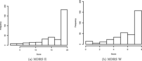
Figure 1: Histograms of scores for MDRS E and W items.

We are interested in modeling the relationship between the primary factor and the volume of white matter hyperintensities located in the frontal lobe of the brain. Controlling for other covariates, we specified the mean of the primary factor as

$$\mathrm{E}[\eta_{i1}]=\beta_{1}\mathrm{Sex}_{i}+\beta_{2}\mathrm{Educ}_{i}+\beta_{3}\mathrm{Age}_{i}+\beta_{4}\mathrm{Vol}_{i}+\beta_{5}\mathrm{WMH}_{i},$$ (36)

where Sex is the participant’s sex (Female${}={}$1, Male${}={}$0), Educ is the number of years of education, Vol is the total brain volume of the participant, and WMH is the frontal white matter hyperintensity volume. We used standardized versions of the continuous predictor variables. Table 2 displays some summary statistics for these covariates by different levels of frontal white matter hyperintensity volume.

Table 2: Mean and SD for covariates by level of frontal WMH. The range of frontal WMH measurements was partitioned to obtain three similarly sized groups

	Frontal WMH (cc)
	0–5	$\bolds{>}$5–11	$\bolds{>}$11
No. participants	113	112	116
Age (Yrs)	68.49 (8.65)	74.82 (6.72)	79.44 (6.23)
Education (Yrs)	15.36 (2.95)	15.12 (3.01)	14.32 (3.12)
Total brain volume (cc)	1196.2 (115.81)	1231.65 (114.78)	1218.34 (138.13)

One-factor semiparametric model. We started our analysis by examining the $Q=1$ model with a single latent factor explaining interdependencies among the test items. To estimate the model, we utilized the parameter-expanded Gibbs sampling algorithm. Even though we found this approach to be more efficient than the standard Gibbs sampler, we still observed high autocorrelation within the chains for factor loadings. We drew 50,000 MCMC samples and discarded the first half as burn-in. We used trace plots and the Geweke [Geweke (1992)] and Raftery–Lewis [Raftery and Lewis (1995)] diagnostic tests to assess convergence.

Table 4 displays posterior summaries for the regression coefficients, $\bolds{\beta}$. We observed a negative relationship between the primary factor and frontal white matter hyperintensity volume. The accompanying 95% posterior credible interval ($-0.466,-0.205$) did not contain zero, suggesting a negative association between frontal white matter hyperintensity volume and the primary factor.

We evaluated model fit using posterior predictive model checks. We began by examining the fit of the marginal distributions. Figure 2 displays the histograms of observed responses for Verbal Fluency outcome $A$ and MDRS outcome $E$ along with posterior predictive summaries. In each case, the model appeared to do a satisfactory job of approximating the data. We found similarly good approximations of the marginal distributions in the observed data for the other outcomes as well.

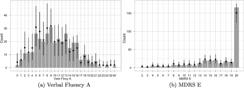
Figure 2: Histograms of the observed scores for the Verbal Fluency $A$ and MDRS $E$. The black points indicate the mean count across replicated data sets for each score. The black vertical segment indicates the interval from the 2.5% to 97.5% quantiles across replicated data sets.

We assessed the model’s ability to replicate the observed dependence structure in the data at a global level by examining the eigenvalues of the observed rank correlation matrix [Figure 3(a)]. The eigenvalues of correlation matrices form the basis of heuristic tests in factor analysis such as the latent root criterion [Guttman (1954)] or the scree test [Cattell (1966)] that determine the number of factors to include in the model. The first eigenvalue was well approximated by the model but the subsequent eigenvalues indicated model misfit, suggesting that additional factors may be necessary to more accurately represent the dependence structure in the data.

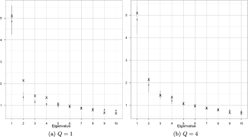
Figure 3: Eigenvalue plots for the $Q=1$ and $Q=4$ models. The mean posterior prediction (grey point) and 95% posterior prediction intervals (grey line segment) of the top ten eigenvalues calculated using replicated data from the single factor ($Q=1$) and bifactor ($Q=4$) models. Eigenvalues computed from the observed data are denoted by a black “$X$.”

We reviewed the pairwise rank correlations to better understand the shortcomings of the single factor model and direct the next steps in our model building process. Figures 4(a) and 4(b) display the pairwise correlation plots for the MDRS J and Visual Span Backward outcomes for the single factor model. In both cases, the model fit the majority of the pairwise correlations well. However, in each case, there were a few outcomes with poorly fitted correlations. For MDRS J, the model did not appear to fully capture the correlation with the conceptually-related MDRS I and K; all three of these outcomes ask participants to repeat alternating movements of some type. Likewise, for Visual Span Backward, the correlation with Visual Span Forward was not accurately approximated by the single factor model. In addition, the correlations between Visual Span Backward and the MDRS outcomes L and O were not well approximated. MDRS outcomes L and O involve copying drawings and, in this sense, also incorporate a visual component that may be the source of the residual correlation between the outcomes. The observation that the lack of fit was present among conceptually related outcomes (e.g., outcomes that are parts of a subtest or a subscale) is consistent with the notion that possible secondary factors may impact item correlations in addition to the general executive functioning factor. Thus, our next step was to consider the class of bifactor models.

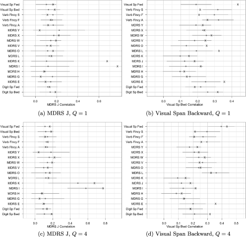
Figure 4: Pairwise correlation plots for the single factor ($Q=1$) and bifactor models ($Q=4$). Each pairwise correlation plot depicts the mean posterior prediction (grey point) and 95% posterior prediction intervals (grey line segment) for Kendall’s $\tau$ values calculated using replicated data. Kendall’s $\tau$ values computed from the observed data are denoted by a black “X.”

Bifactor semiparametric model. To choose a secondary factors structure in a bifactor model, we applied an iterative process. During one iteration, we examined all pairwise correlations for the lack of fit, specified secondary factors to account for residual correlation, refit the model and checked the fit of this new model. Ultimately, we specified a bifactor model with one general cognitive ability factor and 3 secondary factors (for a total of $Q=4$) as listed in Table 3. It is important to note that, although we identified these secondary factors using the posterior predictive model checks, they nevertheless have substantive interpretations as they link conceptually related outcomes. The second factor loads on MDRS outcomes I, J and K, test items that all involve repetition of alternating movements. The third factor loads on the Visual Span outcomes and MDRS outcomes L, O and V. These test items all include visual or drawing components. The fourth factor links three MDRS outcomes that ask participants to identify similarities and dissimilarities.

Table 3: Proposed factor structure for SIVD executive functioning outcomes. $\ast$ indicates a nonzero factor loading to be estimated

	Outcomes
Factor	MDRS G	MDRS H	MDRS I	MDRS J	MDRS K	MDRS L	MDRS O	Digit Sp Fwd	Digit Sp Bwd	Visual Sp Fwd	Visual Sp Bwd	Verb Flncy F	Verb Flncy A	Verb Flncy S	MDRS E	MDRS V	MDRS W	MDRS X	MDRS Y
1	$\ast$	$\ast$	$\ast$	$\ast$	$\ast$	$\ast$	$\ast$	$\ast$	$\ast$	$\ast$	$\ast$	$\ast$	$\ast$	$\ast$	$\ast$	$\ast$	$\ast$	$\ast$	$\ast$
2	0	0	$\ast$	$\ast$	$\ast$	0	0	0	0	0	0	0	0	0	0	0	0	0	0
3	0	0	0	0	0	$\ast$	$\ast$	0	0	$\ast$	$\ast$	0	0	0	0	$\ast$	0	0	0
4	0	0	0	0	0	0	0	0	0	0	0	0	0	0	0	0	$\ast$	$\ast$	$\ast$

Table 4: Posterior summaries for regression coefficients for single factor, $Q=1$, and bifactor, $Q=4$, models

	$\bolds{Q=1}$			$\bolds{Q=4}$
Coefficient	Mean	Median	95% CI	Mean	Median	95% CI
Sex	$0.234$	$0.233$	$(-0.061,0.516)$	$0.155$	$0.152$	$(-0.134,0.440)$
Education	$0.354$	$0.354$	(0.232, 0.479)	$0.325$	$0.325$	(0.206, 0.446)
Age	$-0.126$	$-0.126$	$(-0.246,0.004)$	$-0.078$	$-0.078$	$(-0.201,0.044)$
Total brain Vol.	$0.069$	$0.069$	$(-0.080,0.215)$	$0.046$	$0.045$	$(-0.096,0.194)$
Frontal WMH Vol.	$-0.330$	$-0.328$	$(-0.466,-0.205)$	$-0.335$	$-0.336$	$(-0.464,-0.208)$

For the semiparametric bifactor model with $Q=4$, we drew 500,000 MCMC samples and discarded the first 50,000 as burn-in. We kept every 50th draw, leaving us with 9000 posterior draws. As with the single factor model, we checked convergence using trace plots and the Geweke [Geweke (1992)] and Raftery–Lewis [Raftery and Lewis (1995)] diagnostic tests. Convergence was satisfactory but, compared to the single factor model, the mixing was considerably slower for a few of the secondary factors that exhibited high levels of autocorrelation. We should also note that the speed of convergence was influenced by the choice of hyperparameters for $\bolds{\Sigma}$ and $\bolds{\Psi}$ in the parameter expanded model.

The bifactor model represented the dependence structure of the observed responses better. Figure 3(b) shows that the bifactor model provided a good fit to the observed eigenvalues well beyond the first eigenvalue. As can be seen in Figures 4(c) and 4(d), the bifactor model did a better job of replicating the pairwise rank correlations compared to the single factor model. In Figure 4(c), one may also notice the larger posterior credible intervals for the pairwise rank correlations of MDRS I with MDRS J and MDRS K. Referring back to Table 1, we see that almost all participants answered these items correctly. As a result, there is less information to estimate the secondary factor that accounts for the residual correlation among these three items and, in the wide credible intervals, we see the subsequent imprecision.

Table 4 displays posterior summaries for the regression parameters. We saw little change in our estimate for the parameter of interest, $\beta_{5}$, the coefficient for frontal WMH in adding additional factors. Thus, our substantive conclusion regarding the association between an individual’s executive functioning and the volume of white matter hyperintensities in the frontal region of the brain remains the same whether we use the one-factor model or the better fitting bifactor model. Based on our semiparametric latent variable model, we expect a 1SD increase in frontal white matter hyperintensity volume to be associated with a 0.335SD decrease in the primary factor. In examining the other coefficients, we see that none of the 95% posterior credible intervals have shifted to the extent that we would alter our posterior belief about whether zero is a plausible value for the parameter. However, the coefficients for sex, age and total brain volume did decrease by 30–40% in magnitude.

6 Discussion

In this paper we have developed a semiparametric latent variable model for multivariate mixed outcome data. This model, unlike common parametric latent variable modeling approaches for mixed outcome data [Sammel, Ryan and Legler (1997), Moustaki and Knott (2000), Dunson (2003), Shi and Lee (1998)], does not require the specification of conditional distributions for each outcome given the latent variables. When a data set combines a variety of mixed outcomes, picking appropriate conditional distributions for each outcome encountered in real data, extending the parametric models to account for all cases of distributions, and extending estimation methods appropriately can be labor-intensive. Moreover, specification of outcome conditional distributions given the latent variables may be of little interest by itself in any research setting where the main question is in the relationship between a common factor (or factors) and a covariate of interest. Our proposed semiparametric latent variable framework allows one to model interdependencies among observed mixed outcome variables by specifying an appropriate latent variable model while, at the same time, avoiding the specification of outcome distributions conditional on the common latent variables. We have demonstrated this approach for the single-factor and bifactor models, incorporating a covariate effect on the general factor.

The extended rank likelihood can readily be employed with other latent variable models, including item response theory models [van der Linden and Hambleton (1997)] and structural equation models [Bollen (1989)]. In structural equation models, the focus is often on characterizing the relationship between latent variables and/or between latent variables and fixed covariates as in the case of our hierarchical model. In such cases where the focus is not on the loadings or outcome-related parameters, the proposed semiparametric approach would be quite useful in dealing with mixed outcome data. However, the extended rank likelihood may not be as useful in cases where outcome-specific parameters on the scale of the observed outcomes are of interest. In item response theory models, one is often interested in examining the item difficulty and discrimination parameters to better understand the characteristics of individual test questions. The difficulty parameter, the analogue to the specific mean in the factor model, is not directly identifiable with the extended rank likelihood approach. Nonetheless, one could still carry out posterior inference by relying on the relationship between the difficulty parameter and the latent trait. For example, in a two-parameter item response theory model for binary outcomes, the probability of a positive response when the factor score is set to zero is a one-to-one function of the difficulty parameter. Such an alternative, however, may render the semiparametric approach less convenient for a practitioner who is primarily interested in parameters characterizing the properties of individual outcomes.

We employed the semiparametric latent variable model to study the association between the volume of white matter hyperintensities in the frontal lobe and cognitive testing outcomes related to executive functioning from the Subcortical Ischemic Vascular Dementia (SIVD) study. The semiparametric latent variable model allowed us to analyze the mixed cognitive testing outcomes without requiring the specification of parametric distributions for the outcomes conditional on the latent variables. It has been hypothesized that a greater volume of frontal lobe white matter hyperintensities will be associated with worse executive functioning. Consistent with this hypothesis, we found a negative association between the primary factor in our model and the volume of white matter hyperintensities.

Our model selection process was guided by substantive beliefs that associations among items in the cognitive testing data are primarily driven by the main latent factor but can potentially be influenced by secondary latent factors due to local dependencies among groups of related items. Thus, we started our model-building process by fitting the one-factor semiparametric model and relied on posterior predictive model checks to evaluate model misfit and to guide us in identifying a secondary factor structure for the bifactor model. Our posterior predictive checks approach can therefore be thought of as a method of exploratory bifactor analysis when the secondary factor structure is not known in advance [Jennrich and Bentler (2011)]. It also provides a mechanism by which statistical methodologists can work together with substantive experts to develop models that are theoretically justified and that are consistent with the data. We note, however, that the main conclusion about the association between executive functioning and regional brain volumes was not affected much by the choice of a better fitting bifactor model over the single factor model in our case.

While our proposed model selection process is somewhat ad-hoc, one could explore the use of more formal model fit criteria, other model selection methods or a fully Bayesian approach to determine the factor structure for our semiparametric model. For example, one could use the methods of Knowles and Ghahramani (2011) and Rai and Daumé III (2009) to incorporate the Indian Buffet Process prior to simultaneously estimate the loadings, the loadings structure and the number of factors. Within the bifactor model framework, Jennrich and Bentler (2011) recently proposed using a rotation criterion to explore the secondary factor structure. Dunson et al. (2006) presented a Bayesian model averaging approach that accounts for the uncertainty in the number of factors.

Overall, in our work with the cognitive testing data, we found that the semiparametric model was more elegant and much easier in implementation than the standard parametric approaches for mixed outcome data.

References

- Anderson (2003) {bbook}[mr] \bauthor\bsnmAnderson, \bfnmT. W.\binitsT. W. (\byear2003). \btitleAn Introduction to Multivariate Statistical Analysis, \bedition3rd ed. \bpublisherWiley, \blocationHoboken, NJ. \bidmr=1990662 \bptokimsref \endbibitem
- Bartholomew, Knott and Moustaki (2011) {bbook}[mr] \bauthor\bsnmBartholomew, \bfnmDavid\binitsD., \bauthor\bsnmKnott, \bfnmMartin\binitsM. and \bauthor\bsnmMoustaki, \bfnmIrini\binitsI. (\byear2011). \btitleLatent Variable Models and Factor Analysis: A Unified Approach, \bedition3rd ed. \bpublisherWiley, \blocationChichester. \biddoi=10.1002/9781119970583, mr=2849614 \bptokimsref \endbibitem
- Bollen (1989) {bbook}[mr] \bauthor\bsnmBollen, \bfnmKenneth A.\binitsK. A. (\byear1989). \btitleStructural Equations with Latent Variables. \bpublisherWiley, \blocationNew York. \bidmr=0996025 \bptokimsref \endbibitem
- Cardenas et al. (2001) {barticle}[author] \bauthor\bsnmCardenas, \bfnmV. A.\binitsV. A., \bauthor\bsnmEzekiel, \bfnmF.\binitsF., \bauthor\bsnmDi Sclafani, \bfnmV.\binitsV., \bauthor\bsnmGomberg, \bfnmB.\binitsB. and \bauthor\bsnmFein, \bfnmG.\binitsG. (\byear2001). \btitleReliability of tissue volumes and their spatial distribution for segmented magnetic resonance images. \bjournalPsychiatry Research: Neuroimaging \bvolume106 \bpages193–205. \bptokimsref \endbibitem
- Cattell (1966) {barticle}[author] \bauthor\bsnmCattell, \bfnmR. B.\binitsR. B. (\byear1966). \btitleThe scree test for the number of factors. \bjournalMultivariate Behavioral Research \bvolume1 \bpages245–276. \bptokimsref \endbibitem
- Chui (2007) {barticle}[pbm] \bauthor\bsnmChui, \bfnmHelena C.\binitsH. C. (\byear2007). \btitleSubcortical ischemic vascular dementia. \bjournalNeurol. Clin. \bvolume25 \bpages717–740, vi. \biddoi=10.1016/j.ncl.2007.04.003, issn=0733-8619, mid=NIHMS28661, pii=S0733-8619(07)00059-X, pmcid=2084201, pmid=17659187 \bptokimsref \endbibitem
- Chui et al. (2006) {barticle}[author] \bauthor\bsnmChui, \bfnmH. C.\binitsH. C., \bauthor\bsnmZarow, \bfnmC.\binitsC., \bauthor\bsnmMack, \bfnmW. J.\binitsW. J., \bauthor\bsnmEllis, \bfnmW. G.\binitsW. G., \bauthor\bsnmZheng, \bfnmL.\binitsL., \bauthor\bsnmJagust, \bfnmW. J.\binitsW. J., \bauthor\bsnmMungas, \bfnmD.\binitsD., \bauthor\bsnmReed, \bfnmB. R.\binitsB. R., \bauthor\bsnmKramer, \bfnmJ. H.\binitsJ. H., \bauthor\bsnmDeCarli, \bfnmC. C.\binitsC. C. \betalet al. (\byear2006). \btitleCognitive impact of subcortical vascular and Alzheimer’s disease pathology. \bjournalAnnals of Neurology \bvolume60 \bpages677. \bptokimsref \endbibitem
- Congdon (2003) {bbook}[mr] \bauthor\bsnmCongdon, \bfnmPeter\binitsP. (\byear2003). \btitleApplied Bayesian Modelling. \bpublisherWiley, \blocationChichester. \biddoi=10.1002/0470867159, mr=1990543 \bptokimsref \endbibitem
- Congdon (2006) {bbook}[mr] \bauthor\bsnmCongdon, \bfnmPeter\binitsP. (\byear2006). \btitleBayesian Statistical Modelling, \bedition2nd ed. \bpublisherWiley, \blocationChichester. \biddoi=10.1002/9780470035948, mr=2281386 \bptokimsref \endbibitem
- Dobra and Lenkoski (2011) {barticle}[mr] \bauthor\bsnmDobra, \bfnmAdrian\binitsA. and \bauthor\bsnmLenkoski, \bfnmAlex\binitsA. (\byear2011). \btitleCopula Gaussian graphical models and their application to modeling functional disability data. \bjournalAnn. Appl. Stat. \bvolume5 \bpages969–993. \biddoi=10.1214/10-AOAS397, issn=1932-6157, mr=2840183 \bptokimsref \endbibitem
- Dunn (1973) {barticle}[mr] \bauthor\bsnmDunn, \bfnmJames E.\binitsJ. E. (\byear1973). \btitleA note on a sufficiency condition for uniqueness of restricted factor matrix. \bjournalPsychometrika \bvolume38 \bpages141–143. \bidissn=0033-3123, mr=0345326 \bptokimsref \endbibitem
- Dunson (2003) {barticle}[mr] \bauthor\bsnmDunson, \bfnmDavid B.\binitsD. B. (\byear2003). \btitleDynamic latent trait models for multidimensional longitudinal data. \bjournalJ. Amer. Statist. Assoc. \bvolume98 \bpages555–563. \biddoi=10.1198/016214503000000387, issn=0162-1459, mr=2011671 \bptokimsref \endbibitem
- Dunson et al. (2006) {bmisc}[author] \bauthor\bsnmDunson, \bfnmD. B.\binitsD. B. \betalet al. (\byear2006). \bhowpublishedEfficient Bayesian model averaging in factor analysis. Technical report, Duke Univ., Durham, NC. \bptokimsref \endbibitem
- Erosheva and Curtis (2011) {bmisc}[author] \bauthor\bsnmErosheva, \bfnmE.\binitsE. and \bauthor\bsnmCurtis, \bfnmS. M.\binitsS. M. (\byear2011). \bhowpublishedSpecification of rotational constraints in Bayesian confirmatory factor analysis. Technical Report No. 589, Univ. Washington, Seattle, WA. \bptokimsref \endbibitem
- Geweke (1992) {bincollection}[mr] \bauthor\bsnmGeweke, \bfnmJohn\binitsJ. (\byear1992). \btitleEvaluating the accuracy of sampling-based approaches to the calculation of posterior moments. In \bbooktitleBayesian Statistics, 4 (PeñíScola, 1991) (\beditor\bfnmJ. M.\binitsJ. M. \bsnmBernardo, \beditor\bfnmJ.\binitsJ. \bsnmBerger, \beditor\bfnmA. P.\binitsA. P. \bsnmDawid and \beditor\bfnmJ. F. M.\binitsJ. F. M. \bsnmSmith, eds.) \bpages169–193. \bpublisherOxford Univ. Press, \blocationNew York. \bidmr=1380276 \bptokimsref \endbibitem
- Geweke and Zhou (1996) {barticle}[author] \bauthor\bsnmGeweke, \bfnmJ.\binitsJ. and \bauthor\bsnmZhou, \bfnmG.\binitsG. (\byear1996). \btitleMeasuring the pricing error of the arbitrage pricing theory. \bjournalReview of Financial Studies \bvolume9 \bpages557–587. \bptokimsref \endbibitem
- Ghosh and Dunson (2008) {bincollection}[author] \bauthor\bsnmGhosh, \bfnmJ.\binitsJ. and \bauthor\bsnmDunson, \bfnmD. B.\binitsD. B. (\byear2008). \btitleBayesian model selection in factor analytic models. In \bbooktitleRandom effect and latent variable model selection \bpages151–163. \bpublisherSpringer, \blocationNew York. \bptokimsref \endbibitem
- Ghosh and Dunson (2009) {barticle}[mr] \bauthor\bsnmGhosh, \bfnmJoyee\binitsJ. and \bauthor\bsnmDunson, \bfnmDavid B.\binitsD. B. (\byear2009). \btitleDefault prior distributions and efficient posterior computation in Bayesian factor analysis. \bjournalJ. Comput. Graph. Statist. \bvolume18 \bpages306–320. \biddoi=10.1198/jcgs.2009.07145, issn=1061-8600, mr=2749834 \bptokimsref \endbibitem
- Gruhl, Erosheva and Crane (2010) {bmisc}[author] \bauthor\bsnmGruhl, \bfnmJ.\binitsJ., \bauthor\bsnmErosheva, \bfnmE.\binitsE. and \bauthor\bsnmCrane, \bfnmP.\binitsP. (\byear2010). \bhowpublishedAnalyzing cognitive testing data with extensions of item response theory models. Presented at the Joint Statistical Meetings, Vancouver, Canada, August 3, 2010. \bptokimsref \endbibitem
- Gruhl, Erosheva and Crane (2011) {bmisc}[author] \bauthor\bsnmGruhl, \bfnmJ.\binitsJ., \bauthor\bsnmErosheva, \bfnmE.\binitsE. and \bauthor\bsnmCrane, \bfnmP.\binitsP. (\byear2011). \bhowpublishedA semiparametric Bayesian latent trait model for multivariate mixed type data. In International Meeting of the Pyschometric Society. \bptokimsref \endbibitem
- Guttman (1954) {barticle}[mr] \bauthor\bsnmGuttman, \bfnmLouis\binitsL. (\byear1954). \btitleSome necessary conditions for common-factor analysis. \bjournalPsychometrika \bvolume19 \bpages149–161. \bidissn=0033-3123, mr=0091235 \bptokimsref \endbibitem
- Hachinski et al. (2006) {barticle}[author] \bauthor\bsnmHachinski, \bfnmV.\binitsV., \bauthor\bsnmIadecola, \bfnmC.\binitsC., \bauthor\bsnmPetersen, \bfnmR. C.\binitsR. C., \bauthor\bsnmBreteler, \bfnmM. M.\binitsM. M., \bauthor\bsnmNyenhuis, \bfnmD. L.\binitsD. L., \bauthor\bsnmBlack, \bfnmS. E.\binitsS. E., \bauthor\bsnmPowers, \bfnmW. J.\binitsW. J., \bauthor\bsnmDeCarli, \bfnmC.\binitsC., \bauthor\bsnmMerino, \bfnmJ. G.\binitsJ. G., \bauthor\bsnmKalaria, \bfnmR. N.\binitsR. N. \betalet al. (\byear2006). \btitleNational institute of neurological disorders and stroke—Canadian stroke network vascular cognitive impairment harmonization standards. \bjournalStroke \bvolume37 \bpages2220–2241. \bptokimsref \endbibitem
- Hoff (2007) {barticle}[mr] \bauthor\bsnmHoff, \bfnmPeter D.\binitsP. D. (\byear2007). \btitleExtending the rank likelihood for semiparametric copula estimation. \bjournalAnn. Appl. Stat. \bvolume1 \bpages265–283. \biddoi=10.1214/07-AOAS107, issn=1932-6157, mr=2393851 \bptokimsref \endbibitem
- Hoff (2009) {bbook}[mr] \bauthor\bsnmHoff, \bfnmPeter D.\binitsP. D. (\byear2009). \btitleA First Course in Bayesian Statistical Methods. \bpublisherSpringer, \blocationNew York. \biddoi=10.1007/978-0-387-92407-6, mr=2648134 \bptokimsref \endbibitem
- Holzinger and Swineford (1937) {barticle}[author] \bauthor\bsnmHolzinger, \bfnmK. J.\binitsK. J. and \bauthor\bsnmSwineford, \bfnmF.\binitsF. (\byear1937). \btitleThe bi-factor method. \bjournalPsychometrika \bvolume2 \bpages41–54. \bptokimsref \endbibitem
- Jennrich (1978) {barticle}[mr] \bauthor\bsnmJennrich, \bfnmRobert I.\binitsR. I. (\byear1978). \btitleRotational equivalence of factor loading matrices with specified values. \bjournalPsychometrika \bvolume43 \bpages421–426. \biddoi=10.1007/BF02293650, issn=0033-3123, mr=0514727 \bptokimsref \endbibitem
- Jennrich and Bentler (2011) {barticle}[mr] \bauthor\bsnmJennrich, \bfnmRobert I.\binitsR. I. and \bauthor\bsnmBentler, \bfnmPeter M.\binitsP. M. (\byear2011). \btitleExploratory bi-factor analysis. \bjournalPsychometrika \bvolume76 \bpages537–549. \biddoi=10.1007/s11336-011-9218-4, issn=0033-3123, mr=2851500 \bptokimsref \endbibitem
- Jöreskog (1969) {barticle}[author] \bauthor\bsnmJöreskog, \bfnmK. G.\binitsK. G. (\byear1969). \btitleA general approach to confirmatory maximum likelihood factor analysis. \bjournalPsychometrika \bvolume34 \bpages183–202. \bptokimsref \endbibitem
- Klüppelberg and Kuhn (2009) {barticle}[mr] \bauthor\bsnmKlüppelberg, \bfnmClaudia\binitsC. and \bauthor\bsnmKuhn, \bfnmGabriel\binitsG. (\byear2009). \btitleCopula structure analysis. \bjournalJ. R. Stat. Soc. Ser. B Stat. Methodol. \bvolume71 \bpages737–753. \biddoi=10.1111/j.1467-9868.2009.00707.x, issn=1369-7412, mr=2749917 \bptokimsref \endbibitem
- Knowles and Ghahramani (2011) {barticle}[mr] \bauthor\bsnmKnowles, \bfnmDavid\binitsD. and \bauthor\bsnmGhahramani, \bfnmZoubin\binitsZ. (\byear2011). \btitleNonparametric Bayesian sparse factor models with application to gene expression modeling. \bjournalAnn. Appl. Stat. \bvolume5 \bpages1534–1552. \biddoi=10.1214/10-AOAS435, issn=1932-6157, mr=2849785 \bptokimsref \endbibitem
- Kuczynski et al. (2010) {barticle}[author] \bauthor\bsnmKuczynski, \bfnmB.\binitsB., \bauthor\bsnmTargan, \bfnmE.\binitsE., \bauthor\bsnmMadison, \bfnmC.\binitsC., \bauthor\bsnmWeiner, \bfnmM.\binitsM., \bauthor\bsnmZhang, \bfnmY.\binitsY., \bauthor\bsnmReed, \bfnmB.\binitsB., \bauthor\bsnmChui, \bfnmH. C.\binitsH. C. and \bauthor\bsnmJagust, \bfnmW.\binitsW. (\byear2010). \btitleWhite matter integrity and cortical metabolic associations in aging and dementia. \bjournalAlzheimer’s and Dementia \bvolume6 \bpages54–62. \bptokimsref \endbibitem
- Liu, Rubin and Wu (1998) {barticle}[mr] \bauthor\bsnmLiu, \bfnmChuanhai\binitsC., \bauthor\bsnmRubin, \bfnmDonald B.\binitsD. B. and \bauthor\bsnmWu, \bfnmYing Nian\binitsY. N. (\byear1998). \btitleParameter expansion to accelerate EM: The PX-EM algorithm. \bjournalBiometrika \bvolume85 \bpages755–770. \biddoi=10.1093/biomet/85.4.755, issn=0006-3444, mr=1666758 \bptokimsref \endbibitem
- Liu and Wu (1999) {barticle}[mr] \bauthor\bsnmLiu, \bfnmJun S.\binitsJ. S. and \bauthor\bsnmWu, \bfnmYing Nian\binitsY. N. (\byear1999). \btitleParameter expansion for data augmentation. \bjournalJ. Amer. Statist. Assoc. \bvolume94 \bpages1264–1274. \biddoi=10.2307/2669940, issn=0162-1459, mr=1731488 \bptokimsref \endbibitem
- Loken (2005) {barticle}[mr] \bauthor\bsnmLoken, \bfnmEric\binitsE. (\byear2005). \btitleIdentification constraints and inference in factor models. \bjournalStruct. Equ. Model. \bvolume12 \bpages232–244. \biddoi=10.1207/s15328007sem1202_3, issn=1070-5511, mr=2135915 \bptokimsref \endbibitem
- Lopes and West (2004) {barticle}[mr] \bauthor\bsnmLopes, \bfnmHedibert Freitas\binitsH. F. and \bauthor\bsnmWest, \bfnmMike\binitsM. (\byear2004). \btitleBayesian model assessment in factor analysis. \bjournalStatist. Sinica \bvolume14 \bpages41–67. \bidissn=1017-0405, mr=2036762 \bptokimsref \endbibitem
- Millsap (2001) {barticle}[author] \bauthor\bsnmMillsap, \bfnmR. E.\binitsR. E. (\byear2001). \btitleWhen trivial constraints are not trivial: The choice of uniqueness constraints in confirmatory factor analysis. \bjournalStruct. Equ. Model. \bvolume8 \bpages1–17. \bptokimsref \endbibitem
- Morris (1993) {barticle}[pbm] \bauthor\bsnmMorris, \bfnmJ. C.\binitsJ. C. (\byear1993). \btitleThe Clinical Dementia Rating (CDR): Current version and scoring rules. \bjournalNeurology \bvolume43 \bpages2412–2414. \bidissn=0028-3878, pmid=8232972 \bptokimsref \endbibitem
- Morris (1997) {barticle}[pbm] \bauthor\bsnmMorris, \bfnmJ. C.\binitsJ. C. (\byear1997). \btitleClinical dementia rating: A reliable and valid diagnostic and staging measure for dementia of the Alzheimer type. \bjournalInt. Psychogeriatr. \bvolume9 Suppl 1 \bpages173–176; discussion 177–178. \bidissn=1041-6102, pmid=9447441 \bptnotecheck related\bptokimsref \endbibitem
- Moustaki and Knott (2000) {barticle}[mr] \bauthor\bsnmMoustaki, \bfnmIrini\binitsI. and \bauthor\bsnmKnott, \bfnmMartin\binitsM. (\byear2000). \btitleGeneralized latent trait models. \bjournalPsychometrika \bvolume65 \bpages391–411. \biddoi=10.1007/BF02296153, issn=0033-3123, mr=1792703 \bptokimsref \endbibitem
- Mungas et al. (2005) {barticle}[author] \bauthor\bsnmMungas, \bfnmD.\binitsD., \bauthor\bsnmHarvey, \bfnmD.\binitsD., \bauthor\bsnmReed, \bfnmB. R.\binitsB. R., \bauthor\bsnmJagust, \bfnmW. J.\binitsW. J., \bauthor\bsnmDeCarli, \bfnmC.\binitsC., \bauthor\bsnmBeckett, \bfnmL.\binitsL., \bauthor\bsnmMack, \bfnmW. J.\binitsW. J., \bauthor\bsnmKramer, \bfnmJ. H.\binitsJ. H., \bauthor\bsnmWeiner, \bfnmM. W.\binitsM. W., \bauthor\bsnmSchuff, \bfnmN.\binitsN. \betalet al. (\byear2005). \btitleLongitudinal volumetric MRI change and rate of cognitive decline. \bjournalNeurology \bvolume65 \bpages565–571. \bptokimsref \endbibitem
- Muraki (1992) {barticle}[author] \bauthor\bsnmMuraki, \bfnmE.\binitsE. (\byear1992). \btitleA generalized partial credit model: Application of an EM algorithm. \bjournalAppl. Psychol. Meas. \bvolume16 \bpages159. \bptokimsref \endbibitem
- Murray et al. (2013) {barticle}[author] \bauthor\bsnmMurray, \bfnmJared S.\binitsJ. S., \bauthor\bsnmDunson, \bfnmDavid B.\binitsD. B., \bauthor\bsnmCarin, \bfnmLawrence\binitsL. and \bauthor\bsnmLucas, \bfnmJoseph E.\binitsJ. E. (\byear2013). \btitleBayesian Gaussian copula factor models for mixed data. \bjournalJ. Amer. Statist. Assoc. \bvolume108 \bpages656–665. \bptokimsref \endbibitem
- Pettitt (1982) {barticle}[mr] \bauthor\bsnmPettitt, \bfnmA. N.\binitsA. N. (\byear1982). \btitleInference for the linear model using a likelihood based on ranks. \bjournalJ. R. Stat. Soc. Ser. B Stat. Methodol. \bvolume44 \bpages234–243. \bidissn=0035-9246, mr=0676214 \bptokimsref \endbibitem
- Raftery and Lewis (1995) {bincollection}[author] \bauthor\bsnmRaftery, \bfnmA. E.\binitsA. E. and \bauthor\bsnmLewis, \bfnmS. M.\binitsS. M. (\byear1995). \btitleThe number of iterations, convergence diagnostics and generic Metropolis algorithms. In \bbooktitlePractical Markov Chain Monte Carlo (\beditor\bfnmW. R.\binitsW. R. \bsnmGilks, \beditor\bfnmD. J.\binitsD. J. \bsnmSpiegelhalter and \beditor\bfnmS.\binitsS. \bsnmRichardson, eds.). \bpublisherChapman & Hall, \blocationLondon, UK. \bptokimsref \endbibitem
- Rai and Daumé III (2009) {bmisc}[author] \bauthor\bsnmRai, \bfnmP.\binitsP. and \bauthor\bsnmDaumé III, \bfnmH.\binitsH. (\byear2009). \bhowpublishedThe infinite hierarchical factor regression model. Available at \arxivurlarXiv:0908.0570. \bptokimsref \endbibitem
- Reise, Morizot and Hays (2007) {barticle}[pbm] \bauthor\bsnmReise, \bfnmSteven P.\binitsS. P., \bauthor\bsnmMorizot, \bfnmJulien\binitsJ. and \bauthor\bsnmHays, \bfnmRon D.\binitsR. D. (\byear2007). \btitleThe role of the bifactor model in resolving dimensionality issues in health outcomes measures. \bjournalQual. Life Res. \bvolume16 Suppl 1 \bpages19–31. \biddoi=10.1007/s11136-007-9183-7, issn=0962-9343, pmid=17479357 \bptokimsref \endbibitem
- Samejima (1969) {barticle}[author] \bauthor\bsnmSamejima, \bfnmF.\binitsF. (\byear1969). \btitleEstimation of latent ability using a response pattern of graded scores. \bjournalPsychometrika Monograph Supplement \bvolume34 \bpages1–100. \bptokimsref \endbibitem
- Sammel, Ryan and Legler (1997) {barticle}[author] \bauthor\bsnmSammel, \bfnmM. D.\binitsM. D., \bauthor\bsnmRyan, \bfnmL. M.\binitsL. M. and \bauthor\bsnmLegler, \bfnmJ. M.\binitsJ. M. (\byear1997). \btitleLatent variable models for mixed discrete and continuous outcomes. \bjournalJ. R. Stat. Soc. Ser. B Stat. Methodol. \bvolume59 \bpages667–678. \bptokimsref \endbibitem
- Shi and Lee (1998) {barticle}[author] \bauthor\bsnmShi, \bfnmJ. Q.\binitsJ. Q. and \bauthor\bsnmLee, \bfnmS. Y.\binitsS. Y. (\byear1998). \btitleBayesian sampling-based approach for factor analysis models with continuous and polytomous data. \bjournalBritish J. Math. Statist. Psych. \bvolume51 \bpages233–252. \bptokimsref \endbibitem
- Skrondal and Rabe-Hesketh (2004) {bbook}[mr] \bauthor\bsnmSkrondal, \bfnmAnders\binitsA. and \bauthor\bsnmRabe-Hesketh, \bfnmSophia\binitsS. (\byear2004). \btitleGeneralized Latent Variable Modeling: Multilevel, Longitudinal, and Structural Equation Models. \bpublisherChapman & Hall/CRC, \blocationBoca Raton, FL. \biddoi=10.1201/9780203489437, mr=2059021 \bptokimsref \endbibitem
- Stephens (2000) {barticle}[mr] \bauthor\bsnmStephens, \bfnmMatthew\binitsM. (\byear2000). \btitleDealing with label switching in mixture models. \bjournalJ. R. Stat. Soc. Ser. B Stat. Methodol. \bvolume62 \bpages795–809. \biddoi=10.1111/1467-9868.00265, issn=1369-7412, mr=1796293 \bptokimsref \endbibitem
- van der Linden and Hambleton (1997) {bbook}[mr] \beditor\bparticlevan der \bsnmLinden, \bfnmWim J.\binitsW. J. and \beditor\bsnmHambleton, \bfnmRonald K.\binitsR. K., eds. (\byear1997). \btitleHandbook of Modern Item Response Theory. \bpublisherSpringer, \blocationNew York. \bidmr=1601043 \bptokimsref \endbibitem
- West (1987) {barticle}[mr] \bauthor\bsnmWest, \bfnmMike\binitsM. (\byear1987). \btitleOn scale mixtures of normal distributions. \bjournalBiometrika \bvolume74 \bpages646–648. \biddoi=10.1093/biomet/74.3.646, issn=0006-3444, mr=0909372 \bptokimsref \endbibitem