A hierarchically blocked Jacobi SVD algorithm for single and multiple graphics processing units

Abstract

We present a hierarchically blocked one-sided Jacobi algorithm for the singular value decomposition (SVD), targeting both single and multiple graphics processing units (GPUs). The blocking structure reflects the levels of GPU’s memory hierarchy. The algorithm may outperform MAGMA’s dgesvd, while retaining high relative accuracy. To this end, we developed a family of parallel pivot strategies on GPU’s shared address space, but applicable also to inter-GPU communication. Unlike common hybrid approaches, our algorithm in a single GPU setting needs a CPU for the controlling purposes only, while utilizing GPU’s resources to the fullest extent permitted by the hardware. When required by the problem size, the algorithm, in principle, scales to an arbitrary number of GPU nodes. The scalability is demonstrated by more than twofold speedup for sufficiently large matrices on a Tesla S2050 system with four GPUs vs. a single Fermi card.

1 Introduction

Graphics processing units have become a widely accepted tool of parallel scientific computing, but many of the established algorithms still need to be redesigned with massive parallelism in mind. Instead of multiple CPU cores, which are fully capable of simultaneously processing different operations, GPUs are essentially limited to many concurrent instructions of the same kind—a paradigm known as SIMT (single-instruction, multiple-threads) parallelism.

SIMT type of parallelism is not the only reason for the redesign. Modern CPU algorithms rely on (mostly automatic) multi-level cache management for speedup. GPUs instead offer a complex memory hierarchy, with different access speeds and patterns, and both automatically and programmatically managed caches. Even more so than in the CPU world, a (less) careful hardware-adapted blocking of a GPU algorithm is the key technique by which considerable speedups are gained (or lost).

After the introductory paper [29], here we present a family of the full block [21] and the block-oriented [20] one-sided Jacobi-type algorithm variants for the ordinary (SVD) and the hyperbolic singular value decomposition (HSVD) of a matrix, targeting both a single and the multiple GPUs. The blocking of our algorithm follows the levels of the GPU memory hierarchy; namely, the innermost level of blocking tries to maximize the amount of computation done inside the fastest (and smallest) memory of the registers and manual caches. The GPU’s global RAM and caches are considered by the mid-level, while inter-GPU communication and synchronization are among the issues addressed by the outermost level of blocking.

At each blocking level an instance of either the block-oriented or the full block Jacobi (H)SVD is run, orthogonalizing pivot columns or block-columns by conceptually the same algorithm at the lower level. Thus, the overall structure of the algorithm is hierarchical (or recursive) in nature, and ready to fit not only the current GPUs, but also various other memory and communication hierarchies, provided that efficient, hardware-tuned implementations at each level are available.

The Jacobi method is an easy and elegant way to find the eigenvalues and eigenvectors of a symmetric matrix. In 1958 Hestenes [22] developed the one-sided Jacobi SVD method—an implicit diagonalization is performed by orthogonalizing a factor of a symmetric positive definite matrix. But, after discovery of the QR algorithm in 1961/62 by Francis and Kublanovskaya, the Jacobi algorithm seemed to have no future, at least in the sequential processing world, due to its perceived slowness [17]. However, a new hope for the algorithm has been found in its amenability to parallelization, in its proven high relative accuracy [11], and finally in the emergence of the fast Jacobi SVD implementation in LAPACK, due to Drmač and Veselić [15, 16].

In the beginning of the 1970s Sameh in [33] developed two strategies for parallel execution of the Jacobi method on Illiac IV. The first of those, the modulus strategy, is still in use, and it is one of the very rare parallel strategies for which a proof of convergence exists [26].

In the mid 1980s, Brent and Luk designed another parallel strategy [4], known by the names of its creators. The same authors, together with Van Loan [5], described several parallel one-sided Jacobi and Kogbetliantz (also known as “the two-sided Jacobi”) algorithms. The parallel block Kogbetliantz method is developed in [40].

In 1987 Eberlein [17] proposed two strategies, the round-robin strategy, and another one that depends on the parity of a sweep. A new efficient recursive divide-exchange parallel strategy, specially designed for the hypercube topologies (and, consequently, matrices of order $2^{n}$) is given in [18]. This strategy is later refined by Mantharam and Eberlein in [27] to the block-recursive (BR) strategy.

Two papers by Luk and Park [25, 26] published in 1989 established equivalence between numerous strategies, showing that if one of them is convergent, then all equivalent strategies are convergent. In the same year Shroff and Schreiber [34] showed convergence for a family of strategies called the wavefront ordering, and discussed the parallel orderings weakly equivalent to the wavefront ordering, and thus convergent.

One of the first attempts of a parallel SVD on a GPU is a hybrid one, by Lahabar and Narayanan [24]. It is based on the Golub–Reinsch algorithm, with bidiagonalization and updating of the singular vectors performed on a GPU, while the rest of the bidiagonal QR algorithm is computed on a CPU. In MAGMA, a GPU library of the LAPACK-style routines, dgesvd algorithm is also hybrid, with bidiagonalization (DGEBRD) parallelized on a GPU [39], while for the bidiagonal QR, LAPACK routine DBDSQR is used. We are unaware of any multi-GPU SVD implementations.

In two of our previous papers [37, 36] we discussed the parallel one-sided Jacobi algorithms for the hyperbolic SVD with two and three levels of blocking, respectively. The outermost level is mapped to a ring of CPUs which communicate according to a slightly modified modulus strategy, while the inner two (in the three-level case) are sequential and correspond to the “fast” (L1) and “slow” (L2 and higher) cache levels.

At first glance a choice of the parallel strategy might seem as a technical detail, but our tests at the outermost level have shown that the modified modulus strategy can be two times faster than the round-robin strategy. That motivated us to explore if and how even faster strategies could be constructed, that preserve the accuracy of the algorithm. We present here a class of parallel strategies designed around a conceptually simple but computationally difficult notion of a metric on a set of strategies of the same order. These new strategies can be regarded as generalizations of the Mantharam–Eberlein BR strategy to all even matrix orders, outperforming the Brent and Luk and modified modulus strategies in our GPU algorithm.

However, a parallel strategy alone is not sufficient to achieve decent GPU performance. The standard routines that constitute a block Jacobi algorithm, like the Gram matrix formation, the Cholesky (or the QR) factorization, and the pointwise one-sided Jacobi algorithm itself, have to be mapped to the fast, but in many ways limited shared memory of a GPU, and to the peculiar way the computational threads are grouped and synchronized. Even the primitives that are usually taken for granted, like the numerically robust calculation of a vector’s $2$-norm, present a challenge on a SIMT architecture. Combined with the problems inherent in the block Jacobi algorithms, whether sequential or parallel, like the reliable convergence criterion, a successful design of the Jacobi-type GPU (H)SVD is far from trivial.

In this paper we show that such GPU-centric design is possible and that the Jacobi-type algorithms for a single and the multiple GPUs compare favorably to the present state-of-the-art in the GPU-assisted computation of the (H)SVD. Since all computational work is offloaded to a GPU, we need no significant CPU $\leftrightarrow$ GPU communication nor complex synchronization of their tasks. This facilitates scaling to a large number of GPUs, while keeping their load in balance and communication simple and predictable. While many questions remain open, we believe that the algorithms presented here are a valuable choice to consider when computing the (H)SVD on the GPUs.

The paper is organized as follows. In Section 2 a brief summary of the one-sided Jacobi-type (H)SVD block algorithm variants is given. In Section 3 new parallel Jacobi strategies—nearest to row-cyclic and to column-cyclic are developed. The main part of the paper is Section 4, where a detailed implementation of a single-GPU Jacobi (H)SVD algorithm is described. In Section 5, a proof-of-concept implementation on multiple GPUs is presented. In Section 6, results of the numerical testing are commented. Two appendices complete the paper with a parallel, numerically stable procedure for computing the $2$-norm of a vector, and some considerations about the Jacobi rotation formulas.

2 Jacobi–type SVD algorithm

Suppose that a matrix $G\in\mathbb{F}^{m\times n}$, where $\mathbb{F}$ denotes the real ($\mathbb{R}$) or the complex ($\mathbb{C}$) field, is given. Without loss of generality, we may assume that $m\geq n$. If not, instead of $G$, the algorithm will transform $G^{\ast}$.

If $m\gg n$, or if the column rank of $G$ is less than $n$, then the first step of the SVD is to preprocess $G$ by the QR factorization with column pivoting [13] and, possibly, row pivoting or row presorting,

(1) $$G=P_{r}QRP_{c}=P_{r}Q\begin{bmatrix}R_{0}\\ 0\end{bmatrix}P_{c},$$

where $Q$ is unitary, $R_{0}\in\mathbb{F}^{k\times n}$ is upper trapezoidal with the full row rank $k$, while $P_{r}$ and $P_{c}$ are permutations. If $k<n$, then $R_{0}$ should be factored by the LQ factorization,

(2) $$R_{0}=P^{\prime}_{r}LQ^{\prime}P^{\prime}_{c}=P^{\prime}_{r}\begin{bmatrix}L_{0}&0\end{bmatrix}Q^{\prime}P^{\prime}_{c}.$$

Finally, $L_{0}\in\mathbb{F}^{k\times k}$ is a lower triangular matrix of full rank. From the SVD of $L_{0}$, by (1) and (2), it is easy to compute the SVD of $G$. Thus, we can assume that the initial $G$ is square and of full rank $n$, with $n\geq 2$.

The one-sided Jacobi SVD algorithm for $G$ can be viewed as the implicit two-sided Jacobi algorithm which diagonalizes either $G^{\ast}G$ or $GG^{\ast}$. Let, e.g., $H\mathrel{\mathop{:}}=G^{\ast}G$. Stepwise, a suitably chosen pair of pivot columns $g_{p}$ and $g_{q}$ of $G$ is orthogonalized by postmultiplying the matrix $\begin{bmatrix}g_{p}&g_{q}\end{bmatrix}$ by a Jacobi plane rotation $\widehat{V}_{pq}$, which diagonalizes the $2\times 2$ pivot matrix $\widehat{H}_{pq}$,

(3) $$\widehat{H}_{pq}=\begin{bmatrix}h_{pp}&h_{pq}\\ h_{pq}^{\ast}&h_{qq}\end{bmatrix}=\begin{bmatrix}g_{p}^{\ast}g_{p}&g_{p}^{\ast}g_{q}\\ g_{q}^{\ast}g_{p}&g_{q}^{\ast}g_{q}\end{bmatrix}=\begin{bmatrix}g_{p}^{\ast}\\ g_{q}^{\ast}\end{bmatrix}\begin{bmatrix}g_{p}&g_{q}\end{bmatrix},$$

such that

(4) $$\widehat{V}_{pq}^{\ast}\widehat{H}_{pq}\widehat{V}_{pq}=\mathop{\operator@font diag}\nolimits(\hat{\lambda}_{p},\hat{\lambda}_{q}).$$

In case of convergence, the product of transformation matrices will approach the set of eigenvector matrices. Let $V$ be an eigenvector matrix of $H$. Then

$$\Lambda=V^{\ast}HV=(V^{\ast}G^{\ast})(GV),\quad\Lambda=\mathop{\operator@font diag}\nolimits(\lambda_{1},\lambda_{2},\ldots,\lambda_{n}).$$

The resulting matrix $GV$ has orthogonal columns, and can be written as

(5) $$GV=U\Sigma,$$

where $U$ is unitary and $\Sigma=\Lambda^{1/2}$ is a diagonal matrix of the column norms of $GV$.

The matrix $U$ of the left singular vectors results from scaling the columns of $GV$ by $\Lambda^{-1/2}$, so only the right singular vectors $V$ have to be obtained, either by accumulation of the Jacobi rotations applied to $G$, or by solving the linear system (5) for $V$, with the initial $G$ preserved. The system (5) is usually triangular, since $G$ is either preprocessed in such a form, or already given as a Cholesky factor in an eigenproblem computation. Solving (5) is therefore faster than accumulation of $V$, but it needs more memory and may be less accurate if $G$ is not well-conditioned (see [14]).

The choice of pivot indices $p$, $q$ in successive steps is essential for possible parallelization of the algorithm. We say that two pairs of indices, $(p,q)$ and $(p^{\prime},q^{\prime})$, are disjoint, or non-colliding, if $p\neq q$, $p^{\prime}\neq q^{\prime}$, and $\{p,q\}\cap\{p^{\prime},q^{\prime}\}=\emptyset$. Otherwise, the pairs are called colliding. These definitions are naturally extended to an arbitrary number of pairs. The pairs of indexed objects (e.g., the pairs of matrix columns) are disjoint or (non-)colliding, if such are the corresponding pairs of the objects’ indices.

The one-sided Jacobi approach is better suited for parallelization than the two-sided one, since it can simultaneously process disjoint pairs of columns. This is still not enough to make a respectful parallel algorithm. In the presence of a memory hierarchy, the columns of $G$ and $V$ should be grouped together into block-columns,

(6) $$G=\begin{bmatrix}G_{\mathsf{1}}&G_{\mathsf{2}}&\cdots&G_{\mathsf{b}}\end{bmatrix},\quad V=\begin{bmatrix}V_{\mathsf{1}}&V_{\mathsf{2}}&\cdots&V_{\mathsf{b}}\end{bmatrix}.$$

In order to balance the workload, the block-columns should be (almost) equally sized.

Usually, a parallel task processes two block-columns $G_{\mathsf{p}}$ and $G_{\mathsf{q}}$, i.e., a single pivot block-pair, either by forming the pivot block-matrix $H_{\mathsf{p}\mathsf{q}}$ and its Cholesky factor $R_{\mathsf{p}\mathsf{q}}$,

(7) $$H_{\mathsf{p}\mathsf{q}}=\begin{bmatrix}G_{\mathsf{p}}^{\ast}G_{\mathsf{p}}&G_{\mathsf{p}}^{\ast}G_{\mathsf{q}}\\ G_{\mathsf{q}}^{\ast}G_{\mathsf{p}}&G_{\mathsf{q}}^{\ast}G_{\mathsf{q}}\end{bmatrix}=\begin{bmatrix}G_{\mathsf{p}}^{\ast}\\ G_{\mathsf{q}}^{\ast}\end{bmatrix}\begin{bmatrix}G_{\mathsf{p}}&G_{\mathsf{q}}\end{bmatrix},\quad P^{\ast}H_{\mathsf{p}\mathsf{q}}P=R_{\mathsf{p}\mathsf{q}}^{\ast}R_{\mathsf{p}\mathsf{q}},$$

or by shortening the block-columns $\begin{bmatrix}G_{\mathsf{p}}&G_{\mathsf{q}}\end{bmatrix}$ directly, by the QR factorization,

(8) $$\begin{bmatrix}G_{\mathsf{p}}&G_{\mathsf{q}}\end{bmatrix}P=Q_{\mathsf{p}\mathsf{q}}\begin{bmatrix}R_{\mathsf{p}\mathsf{q}}\\ 0\end{bmatrix}.$$

The diagonal pivoting in the Cholesky factorization, or analogously, the column pivoting in the QR factorization should be employed, if possible (see [37] for further discussion, involving also the hyperbolic SVD case). However, the pivoting in factorizations (7) or (8) may be detrimental to performance of the parallel implementations of the respective factorizations, so their non-pivoted counterparts have to be used in those cases (with $P=I$). Either way, a square pivot factor $R_{\mathsf{p}\mathsf{q}}$ is obtained. Note that the unitary matrix $Q_{\mathsf{p}\mathsf{q}}$ in the QR factorization is not needed for the rest of the Jacobi process, and it consequently does not have to be computed.

Further processing of $R_{\mathsf{p}\mathsf{q}}$ is determined by a variant of the Jacobi algorithm. The following variants are advisable: block-oriented variant (see [20]), when the communication (or memory access) overhead between the tasks is negligible compared to the computational costs, and full block variant (see [21]), otherwise.

In both variants, $R_{\mathsf{p}\mathsf{q}}$ is processed by an inner one-sided Jacobi method. In the block-oriented variant, exactly one (quasi-)sweep of the inner (quasi-)cyclic Jacobi method is allowed. Therefore, $R_{\mathsf{p}\mathsf{q}}$ is transformed to $R_{\mathsf{p}\mathsf{q}}^{\prime}=R_{\mathsf{p}\mathsf{q}}\widetilde{V}_{\mathsf{p}\mathsf{q}}$, with $\widetilde{V}_{\mathsf{p}\mathsf{q}}$ being a product of the rotations applied in the (quasi-)sweep. In the full block variant, the inner Jacobi method computes the SVD of $R_{\mathsf{p}\mathsf{q}}$, i.e., $R_{\mathsf{p}\mathsf{q}}V_{\mathsf{p}\mathsf{q}}=U_{\mathsf{p}\mathsf{q}}\Sigma_{\mathsf{p}\mathsf{q}}$. By $V_{\mathsf{p}\mathsf{q}}^{\prime}$ we denote the transformation matrix, either $\widetilde{V}_{\mathsf{p}\mathsf{q}}$ from the former, or $V_{\mathsf{p}\mathsf{q}}$ from the latter variant.

Especially for the full block variant, the width of the block-columns should be chosen such that $R_{\mathsf{p}\mathsf{q}}$ and $V_{\mathsf{p}\mathsf{q}}^{\prime}$ jointly saturate, without being evicted from, the fast local memory (e.g., the private caches) of a processing unit to which the block-columns $\begin{bmatrix}G_{\mathsf{p}}&G_{\mathsf{q}}\end{bmatrix}$ are assigned. This also allows efficient blocking of the matrix computations in (7) (or (8)) and (9), as illustrated in Subsections 4.1 and 4.4.

Having computed $V_{\mathsf{p}\mathsf{q}}^{\prime}$, the block-columns of $G$ (and, optionally, $V$) are updated,

(9) $$\begin{bmatrix}G_{\mathsf{p}}^{\prime}&G_{\mathsf{q}}^{\prime}\end{bmatrix}=\begin{bmatrix}G_{\mathsf{p}}&G_{\mathsf{q}}\end{bmatrix}V_{\mathsf{p}\mathsf{q}}^{\prime},\quad\begin{bmatrix}V_{\mathsf{p}}^{\prime}&V_{\mathsf{q}}^{\prime}\end{bmatrix}=\begin{bmatrix}V_{\mathsf{p}}&V_{\mathsf{q}}\end{bmatrix}V_{\mathsf{p}\mathsf{q}}^{\prime}.$$

The tasks processing disjoint pairs of block-columns may compute concurrently with respect to each other, up to the local completions of updates (9). A task then replaces (at least) one of its updated block-columns of $G$ by (at least) one updated block-column of $G$ from another task(s). Optionally, the same replacement pattern is repeated for the corresponding updated block-column(s) of $V$. The block-column replacements entail a synchronization of the tasks. The replacements are performed by communication or, on shared-memory systems, by assigning a new pivot block-pair to each of the tasks.

The inner Jacobi method of both variants may itself be blocked, i.e., may divide $R_{\mathsf{p}\mathsf{q}}$ into block-columns of an appropriate width for the next (usually faster but smaller) memory hierarchy level. This recursive blocking principle terminates at the pointwise (non-blocked) Jacobi method, when no advantages in performance could be gained by further blocking. In that way a hierarchical (or multi-level) blocking algorithm is created, with each blocking level corresponding to a distinct communication or memory domain (see [36]).

For example, in the case of a multi-GPU system, we identify access to the global memory (RAM) of a GPU as slow compared to the shared memory and register access, and data exchange with another GPU as slow compared to access to the local RAM. This suggests the two-level blocking for a single-GPU algorithm, and the three-level for a multi-GPU one.

The inner Jacobi method, whether blocked or not, may be sequential or parallel. Both a single-GPU and a multi-GPU algorithm are examples of a nested parallelism.

Similar ideas hold also for the hyperbolic SVD (HSVD). If $G\in\mathbb{F}^{m\times n}$, $m\geq n$, and $\mathop{\operator@font rank}\nolimits(G)=\mathop{\operator@font rank}\nolimits(GJG^{\ast})$, where $J=\mathop{\operator@font diag}\nolimits(\pm 1)$, then the HSVD of $G$ is (see [30, 42])

(10) $$G=U\begin{bmatrix}\Sigma\\ 0\end{bmatrix}V^{\ast},\quad\Sigma=\mathop{\operator@font diag}\nolimits(\sigma_{1},\ldots,\sigma_{n}),\quad\sigma_{1}\geq\sigma_{2}\geq\cdots\sigma_{n}\geq 0.$$

Here, $U$ is a unitary matrix of order $m$, while $V$ is $J$-unitary, (i.e., $V^{\ast}JV=J$) of order $n$. The HSVD in (10) can be computed by orthogonalization of, either the of columns $G^{\ast}$ by trigonometric rotations [12], or the columns of $G$ by hyperbolic rotations [41].

A diagonalization method for the symmetric definite (or indefinite) matrices requires only the partial SVD (or HSVD), i.e., the matrix $V$ is not needed. With the former algorithm, the eigenvector matrix $U$ should be accumulated, but with the latter, it is easily obtainable by scaling the columns of the final $G$. Thus, the hyperbolic algorithm is advantageous for the eigenproblem applications, as shown in [37].

In the sequel we assume that $\mathbb{F}=\mathbb{R}$, but everything, save the computation of the Jacobi rotations and the hardware-imposed block sizes, remains also valid for $\mathbb{F}=\mathbb{C}$.

3 Parallel pivot strategies

In each step of the classical, two-sided Jacobi (eigenvalue) algorithm, the pivot strategy seeks and annihilates an off-diagonal element $h_{pq}$ with the largest magnitude. This approach has been generalized for the parallel two-sided block-Jacobi methods [3]. However, the one-sided Jacobi algorithms would suffer from a prohibitive overhead of forming and searching through the elements of $H$. In the parallel algorithm there is an additional problem of finding $\lfloor n/2\rfloor$ off-diagonal elements with large magnitudes, that can be simultaneously annihilated. Therefore, a cyclic pivot strategy—a repetitive, fixed order of annihilation of all off-diagonal elements of $H$—is more appropriate for the one-sided algorithms.

More precisely, let $\mathsf{P}_{n}$ be the set $\{(i,j)\mid 1\leq i<j\leq n\}$ of all pivot pairs, i.e., pairs of indices of the elements in the strictly upper triangle of a matrix of order $n$, and let $\tau=|\mathsf{P}_{n}|$ be the cardinality of $\mathsf{P}_{n}$. Obviously, $\tau=n(n-1)/2$. A pivot strategy is a function $\mathcal{P}_{n}\colon\mathbb{N}\to\mathsf{P}_{n}$, that associates with each step $k\geq 1$ a pivot pair $(p(k),q(k))$.

If $\mathcal{P}_{n}$ is a periodic function, with the fundamental period $\upsilon$, then, for all $i\geq 1$, the pivot sequences $\mathsf{C}_{i}(\upsilon)=(\mathcal{P}_{n}(k)\mid(i-1)\upsilon+1\leq k\leq i\upsilon)$, of length $\upsilon$, are identical. Consider a case where such a sequence contains all the pivot pairs from $\mathsf{P}_{n}$. Then, if $\upsilon=\tau$, $\mathcal{P}_{n}$ is called a cyclic strategy and $\mathsf{C}_{i}(\upsilon)$ is its $i$-th sweep. Otherwise, if $\upsilon\geq\tau$, $\mathcal{P}_{n}$ is called a quasi-cyclic strategy and $\mathsf{C}_{i}(\upsilon)$ is its $i$-th quasi-sweep.

A Jacobi method is called (quasi-)cyclic if its pivot strategy is (quasi-)cyclic. In the (quasi-)cyclic method the pivot pair therefore runs through all elements of $\mathsf{P}_{n}$ exactly (at least) once in a (quasi-)sweep, and repeats the same sequence until the convergence criteria are met.

We refer the reader to the standard terminology of equivalent, shift-equivalent and weakly equivalent strategies [34]. In the sequel, we identify a (quasi-)cyclic pivot strategy with its first (quasi-)sweep, to facilitate applications of the existing results for finite sequences to the infinite but periodic ones.

A cyclic Jacobi strategy is perfectly parallel (p-strategy) if it allows simultaneous annihilation of as many elements of $H$ as possible. More precisely, let

(11) $$t=\left\lfloor\frac{n}{2}\right\rfloor,\quad s=\begin{cases}n-1,&\text{$n$ even,}\\ n,&\text{$n$ odd,}\end{cases}$$

then exactly $t$ disjoint pivot pairs can be simultaneously processed in each of the $s$ parallel steps (p-steps). As the p-strategies for an even $n$ admit more parallelism within a p-step, i.e., one parallel task more than the p-strategies for $n-1$, with the same number of p-steps in both cases, in the sequel we assume $n$ to be even.

We now provide a definition of a p-strategy closest to a given sequential strategy. The motivation was to explore whether a heuristic based on such a notion could prove valuable in producing fast p-strategies from the well-known row- and column-cyclic sequential strategies. The numerical testing (see Section 6) strongly supports an affirmative answer.

Let $\mathcal{O}$ defines a cyclic pivot strategy. Then, for each pivot pair $(i,j)\in\mathsf{P}_{n}$ there exists an integer $k$ such that $(i,j)=(p(k),q(k))$, where $(p(k),q(k))\in\mathcal{O}$. For any cyclic strategy $\mathcal{O}^{\prime}$, and for each $(p^{\prime}(k),q^{\prime}(k))\in\mathcal{O}^{\prime}$, there is $(p(\ell(k)),q(\ell(k)))\in\mathcal{O}$, such that

(12) $$(p^{\prime}(k),q^{\prime}(k))=(p(\ell(k)),q(\ell(k))).$$

For $1\leq k\leq\tau$, the values $\ell(k)$ are all distinct, and lie between $1$ and $\tau$, inclusive. For a fixed strategy $\mathcal{O}$, this induces a one-to-one mapping $I_{\mathcal{O}}$, from the set of all cyclic strategies on matrices of order $n$ to the symmetric group $\operatorname{\mathsf{Sym}}(\tau)$, as

$$I_{\mathcal{O}}(\mathcal{O}^{\prime})=(\ell(1),\ell(2),\ldots,\ell(k),\ldots,\ell(\tau))\in\operatorname{\mathsf{Sym}}(\tau),$$

with $\ell(k)$ defined as in (12).

Definition 1.

For any two cyclic strategies, $\mathcal{O}_{1}$ and $\mathcal{O}_{2}$, we say that $\mathcal{O}_{1}$ is closer to $\mathcal{O}$ than $\mathcal{O}_{2}$, and denote that by $\mathcal{O}_{1}\preceq_{\mathcal{O}}\mathcal{O}_{2}$, if $I_{\mathcal{O}}(\mathcal{O}_{1})\preceq I_{\mathcal{O}}(\mathcal{O}_{2})$, where $\preceq$ stands for the lexicographic ordering of permutations.

The relation “strictly closer to $\mathcal{O}$”, denoted by $\prec_{\mathcal{O}}$, is defined similarly. Note that $\preceq_{\mathcal{O}}$ is a total order on the finite set of all cyclic strategies with a fixed $n$, and therefore, each non-empty subset (e.g., a subset of all p-strategies) has a least element. Now, take $\mathcal{O}\in\{\mathcal{R}_{n},\mathcal{C}_{n}\}$, where $\mathcal{R}_{n}$ and $\mathcal{C}_{n}$ are the row-cyclic and the column-cyclic strategies, respectively. Then there exists a unique p-strategy $\mathcal{R}_{n}^{\parallel}$ (resp. $\mathcal{C}_{n}^{\parallel}$) that is closest to $\mathcal{R}_{n}$ (resp. $\mathcal{C}_{n}$).

Interpreted in the graph-theoretical setting, a task of finding the closest p-strategy amounts to a recursive application of an algorithm for generating all maximal independent sets (MIS) in lexicographic order (e.g., [23]). Let $\mathsf{G}$ be a simple graph with the vertices enumerated from $1$ to $\tau$, representing pivot pairs from a prescribed cyclic strategy $\mathcal{O}_{n}$, and the edges denoting that two pivot pairs collide (share an index). Note that $|\text{MIS}(\mathsf{G})|\leq t$, where $t$ is defined by (11). Then a $\text{MIS}(\mathsf{G})$ with $t$ vertices is an admissible p-step, and vice versa. The same holds for the graph $\mathsf{G}^{\prime}=\mathsf{G}\setminus S$, where $S$ is any admissible p-step.

Since any permutation of pivot pairs in a p-step generates an equivalent (called step-equivalent) p-strategy, the vertices in each MIS can be assumed to be sorted in ascending order. With a routine next_lex, returning the lexicographically next $\mathrm{MIS}$ with $t$ vertices (or $\emptyset$ if no such sets are left), Alg. 3.1 always produces $\mathcal{O}_{n}^{\parallel}$, the p-strategy closest to $\mathcal{O}_{n}$. Note that, at the suitable recursion depths, next_lex could prepare further candidates in parallel with the rest of the search, and parallel searches could also be launched (or possibly canceled) on the waiting candidates.

Description : Input: the graph $\mathsf{G}$ induced by $\mathcal{O}_{n}$. Output: $\mathcal{O}_{n}^{\parallel}$ (initially $\emptyset$).

boolean gen_strat($\textnormal{{in}}\ \mathsf{G}$);

begin

       if $\mathsf{G}=\emptyset$ then return true;

       // no more pivot pairs (success) begin loop

            $S\leftarrow\textnormal{{next\_lex(}}\textnormal{\emph{$\mathsf{G}$}}\textnormal{{)}}$;

              // take a lexicographically next MIS…

             if $S=\emptyset$ then return false;

             // …but there are none; fail append $S$ to $\mathcal{O}_{n}^{\parallel}$;

              // …else, $S$ is a new p-step candidate

             if gen_strat($\mathsf{G}\setminus S$) then return true;

             // try recursively… remove $S$ from the back of $\mathcal{O}_{n}^{\parallel}$;

              // …and backtrack if failed

            

      end loop ;

end

Algorithm 3.1 MIS-based generation of the p-strategy $\mathcal{O}_{n}^{\parallel}$ closest to $\mathcal{O}_{n}$.

Alg. 3.1, however optimized, might still not be feasible even for the off-line strategy generation, with $n$ sufficiently large. However, there are two remedies: first, no large sizes are needed due to the multi-level blocking; and second, we show in the sequel that it might suffice to generate $\mathcal{R}_{n}^{\parallel}$ (or $\mathcal{C}_{n}^{\parallel}$) only for $n=2o$, with $o$ odd.

Lemma 2.

For all $n$, the sequence of pivot pairs $S_{n}^{(1)}=((2k-1,2k)\mid 1\leq k\leq n/2)$ is the first p-step of $\mathcal{R}_{n}^{\parallel}$ and $\mathcal{C}_{n}^{\parallel}$.

Proof.

Note that $S_{n}^{(1)}$ is an admissible p-step, i.e., there exists a p-strategy having $S_{n}^{(1)}$ as one of its p-steps. For example, the Brent and Luk strategy starts with it.

The first pivot pair in $\mathcal{R}_{n}$ and $\mathcal{C}_{n}$ is $(1,2)$, i.e., $(2k-1,2k)$ for $k=1$. If all pivot pairs in $\mathcal{R}_{n}$ or $\mathcal{C}_{n}$ containing indices $1$ or $2$ are removed, the first pivot pair in the remaining sequence is $(3,4)$, i.e., $(2k-1,2k)$ for $k=2$. Inductively, after selecting the pivot pair $(2\ell-1,2\ell)$, with $\ell<n/2$, and removing all pivot pairs that contain $2k-1$ or $2k$, for all $1\leq k\leq\ell$, the first remaining pivot pair is $(2\ell^{\prime}-1,2\ell^{\prime})$ for $\ell^{\prime}=\ell+1$.   ∎

A matrix of order $2n$ can be regarded at the same time as a block matrix of order $n$ with $2\times 2$ blocks (see Fig. 1). As a consequence of Lemma 2, after the first p-step of either $\mathcal{R}_{2n}^{\parallel}$ or $\mathcal{C}_{2n}^{\parallel}$ (i.e., $S_{2n}^{(1)}$), the diagonal $2\times 2$ blocks are diagonalized, and the off-diagonal blocks are yet to be annihilated.

Once we have the diagonal blocks diagonalized, it is easy to construct the closest block p-strategy $\widetilde{\mathcal{O}}_{2n}^{\parallel}$ from $\mathcal{O}_{n}^{\parallel}$, since each pivot pair of $\mathcal{O}_{n}^{\parallel}$ corresponds uniquely to an off-diagonal $2\times 2$ block. A p-step of $\mathcal{O}_{n}^{\parallel}$ is expanded to two successive p-steps of $\widetilde{\mathcal{O}}_{2n}^{\parallel}$. The expansion procedure is given by Alg. 3.2, for $\mathcal{O}_{n}\in\{\mathcal{R}_{n},\mathcal{C}_{n}\}$, and illustrated, for $n=6$ and $\mathcal{O}_{n}=\mathcal{R}_{n}$, with Fig. 1. Note that a pivot pair of $\mathcal{O}_{n}^{\parallel}$ contributes two pairs, $(\text{{nw}},\text{{se}})$ and either $(\text{{ne}},\text{{sw}})$ or $(\text{{sw}},\text{{ne}})$, of non-colliding and locally closest pivot pairs in its corresponding block.

Description : Input: $\mathcal{O}_{n}^{\parallel}$, $\mathcal{O}_{n}\in\{\mathcal{R}_{n},\mathcal{C}_{n}\}$. Output: $\widetilde{\mathcal{O}}_{2n}^{\parallel}$.

$S_{n}^{(i)}$ is the $i$-th p-step of $\mathcal{O}_{n}^{\parallel}$, and $S_{2n}^{(i)}$ is the $i$-th p-step of $\widetilde{\mathcal{O}}_{2n}^{\parallel}$.

$S_{2n}^{(1)}\leftarrow((2k-1,2k)\mid 1\leq k\leq n)$;

for $i\leftarrow 2$ to $2n-1$ do // construct $S_{2n}^{(i)}$

      $S_{2n}^{(i)}=\emptyset$;

       foreach $(p,q)\in S_{n}^{(i\operatorname{\mathbf{div}}2)}$ do

            if even($i$) then

                  $\text{{nw}}=(2p-1,2q-1);\quad\text{{se}}=(2p,2q);$ append $(\text{{nw}},\text{{se}})$ to $S_{2n}^{(i)}$;

            else

                  $\text{{ne}}=(2p-1,2q);\quad\text{{sw}}=(2p,2q-1)$;

                   if $\mathcal{O}_{n}=\mathcal{R}_{n}$ then append $(\text{{ne}},\text{{sw}})$ to $S_{2n}^{(i)}$ else append $(\text{{sw}},\text{{ne}})$ to $S_{2n}^{(i)}$;

                  

             end if

            

       end foreach

      

end for

Algorithm 3.2 Expansion of $\mathcal{O}_{n}^{\parallel}$ to $\widetilde{\mathcal{O}}_{2n}^{\parallel}$ for $\mathcal{O}_{n}\in\{\mathcal{R}_{n},\mathcal{C}_{n}\}$.

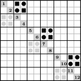
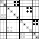
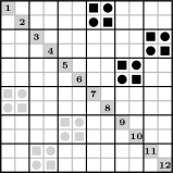
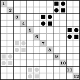
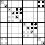
Fig. 1: Expansion of $\mathcal{R}_{6}^{\parallel}$ to $\mathcal{R}_{12}^{\parallel}$, according to Alg. 3.2. From left to right: the black disks represent the odd p-steps, while the black squares stand for the even p-steps.

It’s trivial to show that, with $\mathcal{O}_{n}^{\parallel}$ given, the p-strategy $\widetilde{\mathcal{O}}_{2n}^{\parallel}$ generated by Alg. 3.2 is indeed the closest block p-strategy; any other such $\mathcal{S}_{2n}^{\parallel}\prec_{\mathcal{O}}\widetilde{\mathcal{O}}_{2n}^{\parallel}$ would induce, by the block-to-pivot correspondence, a strategy $\mathcal{S}_{n}^{\parallel}\prec_{\mathcal{O}}\mathcal{O}_{n}^{\parallel}$, which is impossible. Moreover, we have verified that, for $n\leq 18$ and both $\mathcal{R}_{n}$ and $\mathcal{C}_{n}$ strategies, $\widetilde{\mathcal{O}}_{2n}^{\parallel}=\mathcal{O}_{2n}^{\parallel}$, and although lacking a rigorous proof, claim that the same holds for all even $n$. Therefore, as a tentative corrolary, to construct $\mathcal{O}_{m}^{\parallel}$, for $\mathcal{O}_{m}\in\{\mathcal{R}_{m},\mathcal{C}_{m}\}$ and $m=2^{k}o$, with $k>1$ and $o$ odd, it would suffice to construct $\mathcal{O}_{n}^{\parallel}$, $n=2o$, and apply, $k-1$ times, Alg. 3.2.

For example, a three-level blocking algorithm for $4$ GPUs and a matrix of order $15\cdot 1024$ requires $\mathcal{O}_{8}^{\parallel}$, $\mathcal{O}_{240}^{\parallel}$, and $\mathcal{O}_{32}^{\parallel}$ strategies. To find $\mathcal{O}_{240}^{\parallel}$, it suffices to construct $\mathcal{O}_{30}^{\parallel}$, and expand (i.e., duplicate) it $3$ times, since $240=2^{3}\cdot 2\cdot 15$. Thus, the $\mathcal{O}_{m}^{\parallel}$ strategies should be pretabulated once, for the small, computationally feasible orders $m$, and stored into a code library for future use. The expansion procedure can be performed at run-time, when the size of input is known.

The strategies just described progress from the diagonal of a matrix outwards. However, if the magnitudes of the off-diagonal elements in the final sweeps of the two-sided Jacobi method are depicted, a typical picture [16, page 1349] shows that the magnitudes rise towards the ridge on the diagonal. That motivated us to explore whether a faster decay of the off-diagonal elements far away from the diagonal could be reached by annihilating them first, and the near-diagonal elements last. This change of the annihilation order is easily done by reverting the order of pivot pairs in a sweep of $\widetilde{\mathcal{R}}_{n}^{\parallel}$ and $\widetilde{\mathcal{C}}_{n}^{\parallel}$. Formally, a reverse of the strategy $\mathcal{O}_{n}$ is the strategy $\text{\reflectbox{$\mathcal{O}$}}_{n}$, given by

$$\text{\reflectbox{$\mathcal{O}$}}_{n}\mathrel{\mathop{:}}=((p(\tau-k+1),q(\tau-k+1))\mid 1\leq k\leq\tau),$$

where $\mathcal{O}_{n}=((p(k),q(k))\mid 1\leq k\leq\tau)$. Thus, $\text{\reflectbox{$\mathcal{R}$}}_{n}^{\parallel}$ and $\text{\reflectbox{$\mathcal{C}$}}_{n}^{\parallel}$ progress inwards, ending with $S_{n}^{(1)}$ reversed. We tentatively denote the reverses of both $\mathcal{R}_{n}^{\parallel}$ and $\widetilde{\mathcal{R}}_{n}^{\parallel}$ (resp. $\mathcal{C}_{n}^{\parallel}$ and $\widetilde{\mathcal{C}}_{n}^{\parallel}$) by the same symbol.

For $m=2^{k}$, both $\mathcal{R}_{m}^{\parallel}$ and $\mathcal{C}_{m}^{\parallel}$ can be generated efficiently by Alg. 3.1, since no backtracking occurs. In this special case it holds that $\mathcal{R}_{m}^{\parallel}=\widetilde{\mathcal{R}}_{m}^{\parallel}$, $\mathcal{C}_{m}^{\parallel}=\widetilde{\mathcal{C}}_{m}^{\parallel}$, and $\mathcal{R}_{m}^{\parallel}$ is step-equivalent to $\mathcal{C}_{m}^{\parallel}$. The former claims are verified for $k\leq 14$.

The respective reverses, $\text{\reflectbox{$\mathcal{R}$}}_{m}^{\parallel}$ and $\text{\reflectbox{$\mathcal{C}$}}_{m}^{\parallel}$, operate in the same block-recursive fashion (preserved by Alg. 3.2) of the Mantharam–Eberlein BR strategy [27], i.e., processing first the off-diagonal block, and then simultaneously the diagonal blocks of a matrix. It follows that all three strategies are step-equivalent. Thus, $\text{\reflectbox{$\mathcal{R}$}}_{n}^{\parallel}$ and $\text{\reflectbox{$\mathcal{C}$}}_{n}^{\parallel}$ can be regarded as the generalizations of the BR strategy to an arbitrary even order $n$, albeit lacking a simple communication pattern. Conversely, for the power-of-two orders, $\text{\reflectbox{$\mathcal{R}$}}_{m}^{\parallel}$ and $\text{\reflectbox{$\mathcal{C}$}}_{m}^{\parallel}$ might be replaced by the BR strategy with a hypercube-based communication.

4 A single-GPU algorithm

In this section we describe the two-level blocked Jacobi (H)SVD algorithm for a single GPU. The algorithm is designed and implemented with NVIDIA CUDA [7] technology, but is also applicable to OpenCL, and—at least conceptually—to the other massively parallel accelerator platforms.

We assume that the following CUDA operations are correctly rounded, as per IEEE 754-2008 standard [31]: ${+}$, ${-}$, ${*}$, ${/}$, $\sqrt{x}$, $\operatorname{\mathtt{fma}}(x,y,z)=x\cdot y+z$, and $\operatorname{\mathtt{rcp}}(x)=1/x$. Under that assumption, the algorithm may work in any floating-point precision available, but is tested in double precision only, on Fermi and Kepler GPU architectures.

The algorithm performs all computation on a GPU, and consists of $3$ kernels:

1. initV – optional initialization of the matrix $V$ to $I_{n}$, if the full (H)SVD is requested (for the HSVD, $V^{-T}=JVJ$ will be accumulated instead of $V$);

2. pStep – invoked once for each p-step in a block-sweep;

3. Sigma – a final singular value extraction ($\sigma_{i}=\|g^{\prime}_{i}\|_{2}$).

The CPU is responsible only for the main control flow, i.e., kernel invocations and testing of the stopping criterion. Besides a simple statistics from each pStep call, there is no other CPU $\leftrightarrow$ GPU data transfer. We assume that the input factor $G$ is preloaded onto a GPU. We keep the matrix $J$ partitioned as $J=\mathop{\operator@font diag}\nolimits(I,-I)$ and represent it with a parameter $n_{+}$, where $n_{+}$ denotes the number of positive signs in $J$. The output data remaining on the GPU are $G^{\prime}=U\Sigma$ (overwrites $G$), $\Sigma$, and (optionally) $V$.

Data layout (i.e., array order) is column-major (as in Fortran), to be compatible with (cu)BLAS and other numerical libraries, like MAGMA. We write one-based array indices in parentheses, and zero-based ones in square brackets.

The matrices $G$ and $V$ are partitioned into $\mathsf{b}=n/16$ block-columns, as in (6). To simplify the algorithm, $n$ must be divisible by $16$ and $\mathsf{b}$ must be even. Otherwise, if $n$ is not divisible by $32$, $G$ has to be bordered as in [29, eq. (4.1)]. The reason lies in the hardware constraints on the GPU shared memory configurations and a fixed warp size ($32$ threads), as explained in the sequel.

We focus on pStep kernel, since the other two are straightforward. An execution grid for pStep comprises $\mathsf{b}/2$ thread blocks, i.e., one thread block per a pivot block-pair. Each 2-dimensional thread block is assigned $32\times 16=512$ threads, and $16\rm\ kB$ of the GPU shared memory. That imposes a theoretical limit of $3$ thread blocks per multiprocessor, $100\%$ occupancy on a Fermi, and $75\%$ occupancy on a Kepler GPU.

A chosen block p-strategy $\mathcal{S}_{\mathsf{b}}$ is preloaded in the constant or global GPU memory in a form of an $O(1)$ lookup table $S_{\mathsf{b}}$. A thread block $\mathsf{t}$ in a pStep invocation $\mathsf{s}$ during a block-sweep $\mathsf{r}$ obtains from $S_{\mathsf{b}}$ the indices $\mathsf{p}$ and $\mathsf{q}$, $1\leq\mathsf{p}<\mathsf{q}\leq\mathsf{b}$, of the block-columns $\mathsf{t}$ is about to process. In other words, a mapping $(\mathsf{r},\mathsf{s},\mathsf{t})\mapsto(\mathsf{p},\mathsf{q})\in\mathcal{S}_{\mathsf{b}}$ establishes a correspondence between the thread blocks and the pivot block-pairs.

A thread block behavior is uniquely determined by the block indices $\mathsf{p}$ and $\mathsf{q}$, since the thread blocks in every pStep invocation are mutually independent. Computation in a thread block proceeds in the three major phases:

1. factorize – shortens the pivot block-pair $\begin{bmatrix}G_{\mathsf{p}}&G_{\mathsf{q}}\end{bmatrix}$, according to (7) or (8), into the triangular factor $R_{\mathsf{p}\mathsf{q}}$ of order $32$, and initializes $V_{\mathsf{p}\mathsf{q}}^{\prime}=I_{32}$;

2. orthogonalize – orthogonalizes $R_{\mathsf{p}\mathsf{q}}$ by the inner pointwise Jacobi method, according to the block-oriented or the full block variant of the Jacobi (H)SVD algorithm (see Section 2), accumulating the applied rotations into $V_{\mathsf{p}\mathsf{q}}^{\prime}$;

3. postmultiply – postmultiplies $\begin{bmatrix}G_{\mathsf{p}}&G_{\mathsf{q}}\end{bmatrix}$, and optionally $\begin{bmatrix}V_{\mathsf{p}}&V_{\mathsf{q}}\end{bmatrix}$, by $V_{\mathsf{p}\mathsf{q}}^{\prime}$, according to (9).

The matrices $R_{\mathsf{p}\mathsf{q}}$ and $V_{\mathsf{p}\mathsf{q}}^{\prime}$ reside in the shared memory, and together occupy $16\rm\ kB$. The entire allocated shared memory may also be regarded as a single $64\times 32$ double precision matrix, named $G_{\mathsf{p}\mathsf{q}}$, of which $R_{\mathsf{p}\mathsf{q}}$ aliases the lower, and $V_{\mathsf{p}\mathsf{q}}^{\prime}$ the upper half.

There is no shared memory configuration that can hold two square double precision matrices of order that is a larger multiple of the warp size than $32$. It is therefore optimal to use the smallest shared memory configuration ($16\rm\ kB$), leaving the highest amount ($48\rm\ kB$) of the L1 cache available. Also, since $R_{\mathsf{p}\mathsf{q}}$ and $V_{\mathsf{p}\mathsf{q}}^{\prime}$ have to be preserved between the phases, all phases need to be completed in the same kernel invocation. That creates a heavy register pressure, which is the sole reason why only one thread block (instead of $3$) can be active on a multiprocessor.

In the complex case ($\mathbb{F}=\mathbb{C}$), the shared memory configuration would be $48\rm\ kB$ (suboptimal, $16\rm\ kB$ unutilized) or $32\rm\ kB$, for a Fermi or a Kepler GPU, respectively.

We present two approaches for factorize. The Cholesky factorization of the Gram matrix $H_{\mathsf{p}\mathsf{q}}$, as in (7), is described in Subsection 4.1 in two subphases, and the QR factorization (8) is discussed in Subsection 4.2.

4.1 The Cholesky factorization

The first subphase of factorize loads the successive $64\times 32$ chunks of $\begin{bmatrix}G_{\mathsf{p}}&G_{\mathsf{q}}\end{bmatrix}$ into $G_{\mathsf{p}\mathsf{q}}$. For a thread with the Cartesian indices $[x,y]$ in our thread block, $x$ is its lane ID, and $y$ its warp ID. Let $y^{\prime}=y+16$ onwards. After a chunk is loaded, the thread $[x,y]$ then updates $H_{\mathsf{p}\mathsf{q}}[x,y]$ and $H_{\mathsf{p}\mathsf{q}}[x,y^{\prime}]$ (kept in its registers and being initially $0$),

$$H_{\mathsf{p}\mathsf{q}}[x,y]\mathop{{+}{=}}G_{\mathsf{p}\mathsf{q}}[{:},x]^{T}G_{\mathsf{p}\mathsf{q}}[{:},y],\quad H_{\mathsf{p}\mathsf{q}}[x,y^{\prime}]\mathop{{+}{=}}G_{\mathsf{p}\mathsf{q}}[{:},x]^{T}G_{\mathsf{p}\mathsf{q}}[{:},y^{\prime}].$$

Finally, when all the chunks are processed, $H_{\mathsf{p}\mathsf{q}}$ is written into $R_{\mathsf{p}\mathsf{q}}$, and $V_{\mathsf{p}\mathsf{q}}^{\prime}$ is set to $I_{32}$. Note that data in the GPU RAM are accessed only once. No symmetrization is needed for $H_{\mathsf{p}\mathsf{q}}$, since only its lower triangle is taken as an input for the Cholesky factorization. For details of this subphase see Alg. 4.1.

Description : Input: $\begin{bmatrix}G_{\mathsf{p}}&G_{\mathsf{q}}\end{bmatrix}$. Output: $H_{\mathsf{p}\mathsf{q}}$. Thread ID: $[x,y]$.

$x^{\prime}=x+32;\quad y^{\prime}=y+16;\quad h_{xy}=h_{xy^{\prime}}=0$;

  // $H_{\mathsf{p}\mathsf{q}}$ elements kept in registers

for $(i=x;\,i<n;\,i\mathop{{+}{=}}64)$ // process the next chunk of $\begin{bmatrix}G_{\mathsf{p}}&G_{\mathsf{q}}\end{bmatrix}$

      $G_{\mathsf{p}\mathsf{q}}[x,y]=G_{\mathsf{p}}[i,y];\quad G_{\mathsf{p}\mathsf{q}}[x,y^{\prime}]=G_{\mathsf{q}}[i,y]$;

        // load the first $32$ chunk rows

       if $(i^{\prime}=i+32)<n$ then // load the remaining chunk rows

            $G_{\mathsf{p}\mathsf{q}}[x^{\prime},y]=G_{\mathsf{p}}[i^{\prime},y];\quad G_{\mathsf{p}\mathsf{q}}[x^{\prime},y^{\prime}]=G_{\mathsf{q}}[i^{\prime},y]$;

      else // border $G_{\mathsf{p}\mathsf{q}}$ with zeros

            $G_{\mathsf{p}\mathsf{q}}[x^{\prime},y]=0;\quad G_{\mathsf{p}\mathsf{q}}[x^{\prime},y^{\prime}]=0$;

       end if

       __syncthreads();

        // ensure the shared memory writes have taken effect

       unrolled for $(j=0;\,j<64;\,{+}{+}j)$ // compute the partial dot-products

            $j^{\prime}=(x+j)\bmod 64$;

              // modular row addressing avoids bank conflicts

             $g_{j^{\prime}x}=G_{\mathsf{p}\mathsf{q}}[j^{\prime},x];\quad g_{j^{\prime}y}=G_{\mathsf{p}\mathsf{q}}[j^{\prime},y];\quad g_{j^{\prime}y^{\prime}}=G_{\mathsf{p}\mathsf{q}}[j^{\prime},y^{\prime}]$;

             $h_{xy}=\operatorname{\mathtt{fma}}(g_{j^{\prime}x},g_{j^{\prime}y},h_{xy})$;

              // update $H_{\mathsf{p}\mathsf{q}}[x,y]$

             $h_{xy^{\prime}}=\operatorname{\mathtt{fma}}(g_{j^{\prime}x},g_{j^{\prime}y^{\prime}},h_{xy^{\prime}})$;

              // update $H_{\mathsf{p}\mathsf{q}}[x,y^{\prime}]$

            

       endfor

      __syncthreads();

        // ensure that $G_{\mathsf{p}\mathsf{q}}$ is free to be overwritten

      

endfor

$R_{\mathsf{p}\mathsf{q}}[x,y]=h_{xy};\quad R_{\mathsf{p}\mathsf{q}}[x,y^{\prime}]=h_{xy^{\prime}}$;

  // store (unsymmetrized) $H_{\mathsf{p}\mathsf{q}}$ to $R_{\mathsf{p}\mathsf{q}}$

__syncthreads();

  // ensure the shared memory writes have taken effect

Algorithm 4.1 Device function that computes the Gram matrix $H_{\mathsf{p}\mathsf{q}}$.

On a Kepler GPU, with $8$ bytes wide shared memory banks, each thread in a warp can access a different bank. Due to column-major data layout, each of $32$ consecutive (modulo $64$) rows of $G_{\mathsf{p}\mathsf{q}}$ belongs to a separate bank. Therefore, the modular row addressing of Alg. 4.1 guarantees bank-conflict-free operation on a Kepler GPU, and generates $2$-way bank conflicts on a Fermi GPU, with $4$ bytes wide banks.

The next subphase consists of the in-place, forward-looking Cholesky factorization of $H_{\mathsf{p}\mathsf{q}}$ without pivoting, i.e., $H_{\mathsf{p}\mathsf{q}}=L_{\mathsf{p}\mathsf{q}}L_{\mathsf{p}\mathsf{q}}^{T}$. The factorization proceeds columnwise to avoid bank conflicts. After the factorization, the upper triangle of $R_{\mathsf{p}\mathsf{q}}$ is set to $L_{\mathsf{p}\mathsf{q}}^{T}$, and the strict lower triangle to zero. This transposition is the only part of the entire algorithm that necessarily incurs the bank conflicts. The factorization has $32$ steps. The step $k$, for $0\leq k<32$, transforms $H_{\mathsf{p}\mathsf{q}}[k{:},k{:}]$ in $2$ or $3$ stages:

1. Compute $L_{\mathsf{p}\mathsf{q}}[k{:},k]$, overwriting $H_{\mathsf{p}\mathsf{q}}[k{:},k]$ (see Fig. 2(a)). Only one warp is active. The thread $[x,y]$ performs the following operations:

   • If $x=y=k$, then $L_{\mathsf{p}\mathsf{q}}[k,k]=\sqrt{H_{\mathsf{p}\mathsf{q}}[k,k]}$;

   • else, if $x>y=k$, then $L_{\mathsf{p}\mathsf{q}}[x,k]=H_{\mathsf{p}\mathsf{q}}[x,k]/\sqrt{H_{\mathsf{p}\mathsf{q}}[k,k]}$;

   • else, the thread is dormant, i.e., does nothing.

2. Update at most $16$ subsequent columns of $H_{\mathsf{p}\mathsf{q}}$. Let $j=(k+1)+y$. If $x\geq j$ and $j<32$, then $H_{\mathsf{p}\mathsf{q}}[x,j]=\operatorname{\mathtt{fma}}(-L_{\mathsf{p}\mathsf{q}}[x,k],L_{\mathsf{p}\mathsf{q}}[j,k],H_{\mathsf{p}\mathsf{q}}[x,j])$, else do nothing (see Fig. 2(b)).

3. If there are more columns remaining, let $j^{\prime}=(k+1)+y^{\prime}$. If $x\geq j^{\prime}$ and $j^{\prime}<32$, then $H_{\mathsf{p}\mathsf{q}}[x,j^{\prime}]=\operatorname{\mathtt{fma}}(-L_{\mathsf{p}\mathsf{q}}[x,k],L_{\mathsf{p}\mathsf{q}}[j^{\prime},k],H_{\mathsf{p}\mathsf{q}}[x,j^{\prime}])$, else do nothing (see Fig. 2(c)).

After each stage, a thread-block-wide synchronization (__syncthreads) is necessary.

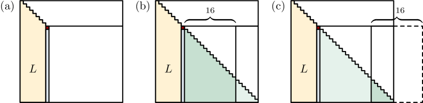
Fig. 2: The forward-looking Cholesky factorization $H_{\mathsf{p}\mathsf{q}}=L_{\mathsf{p}\mathsf{q}}L_{\mathsf{p}\mathsf{q}}^{T}$.

4.2 The QR factorization

When the input matrix $G$ is badly scaled, the QR factorization (8) is required at all blocking levels, since the input columns of too large (resp. too small) norm could cause overflow (resp. underflow) while forming the Gram matrices. If the QR factorization employs the Householder reflectors, the column norm computations should be carried out carefully, as detailed in Appendix A.

The tall-and-skinny in-GPU QR factorization is described in [2]. It is applicable when a single QR factorization per p-step is to be performed on a GPU, e.g., in the shortening phase of a multi-GPU algorithm. On the shared memory blocking level, each thread block has to perform its own QR factorization. Therefore, an algorithm for the batched tall-and-skinny QRs is needed in this case.

Ideally, such an algorithm should access the GPU RAM as few times as possible, and be comparable in speed to the Cholesky factorization approach. We show that the algorithm can be made to access $\begin{bmatrix}G_{\mathsf{p}}&G_{\mathsf{q}}\end{bmatrix}$ exactly once, but the latter remains difficult to accomplish.

Let $A_{0}^{(i)}$ and $A_{1}^{(i)}$ be the $32\times 32$ matrices that alias the lower and the upper half of $G_{\mathsf{p}\mathsf{q}}$, i.e., $R_{\mathsf{p}\mathsf{q}}$ and $V_{\mathsf{p}\mathsf{q}}^{\prime}$, respectively. The first $32\times 32$ chunk of $\begin{bmatrix}G_{\mathsf{p}}&G_{\mathsf{q}}\end{bmatrix}$ is loaded into $A_{0}^{(0)}$ and factorized as $A_{0}^{(0)}=Q_{0}^{(0)}R_{0}^{(0)}$. The factorization is performed by $31$ successive applications of the Householder reflectors, in a pattern similar to Fig. 2(b,c). A reflector is simultaneously computed in all active warps before the update, but is not preserved, and $Q_{0}^{(0)}$ is not (explicitly or implicitly) formed.

More precisely, for $0\leq k<31$, let $H_{k}$ be the reflector annihilating the subdiagonal of the $k$-th column, $H_{k}=I_{32}-\tau_{k}w_{k}w_{k}^{T}$, where $w_{k}=\begin{bmatrix}\mathbf{0}&1&v_{k}\end{bmatrix}^{T}$ ($\mathbf{0}$ is a vector of $k$ zeros). In a thread with the row index $x$, $H_{k}$ is represented by $\tau_{k}$ and $w_{k}[x]$. When the reflector is found, the warp $y$ transforms $A_{0}^{(0)}[\ell{:},\ell]$, where $\ell=k+y$. Let $z_{\ell}$ be the scalar product $z_{\ell}=w_{\ell}^{T}A_{0}^{(0)}[{:},\ell]$, computed by warp-level shared memory reduction (on Fermi), or by warp shuffle reduction (on Kepler). Then, the update by $H_{k}$ is

$$A_{0}^{(0)}[x,\ell]^{\prime}=\operatorname{\mathtt{fma}}(-\tau_{\ell}*z_{\ell},w_{\ell}[x],A_{0}^{(0)}[x,\ell]).$$

The transformation is then repeated for $\ell^{\prime}=k+y^{\prime}$.

After $R_{0}^{(0)}$ is formed, the second chunk of $\begin{bmatrix}G_{\mathsf{p}}&G_{\mathsf{q}}\end{bmatrix}$ is loaded into $A_{1}^{(0)}$ and similarly factored as $A_{1}^{(0)}=Q_{1}^{(0)}R_{1}^{(0)}$.

The factors $R_{0}^{(0)}$ and $R_{1}^{(0)}$ are combined into $R_{0}^{(1)}$ by a “peel-off” procedure illustrated with Fig. 3. The procedure peels off one by one (super)diagonal of $R_{1}^{(0)}$ by the independent Givens rotations, until (after $32$ stages) $R_{1}^{(0)}$ is reduced to a zero matrix. In the stage $k$, the row $x$ of $R_{0}^{(0)}$ and the row $x-k$ of $R_{1}^{(0)}$ are transformed by a rotation determined from $R_{0}^{(0)}[x,x]$ and $R_{1}^{(0)}[x-k,x]$ to annihilate the latter. This is the main conceptual difference from the tall-and-skinny QR, described, e.g., in [9, 10], where the combining is performed by the structure-aware Householder reflectors. The Givens rotations are chosen to avoid the expensive column norm computations.

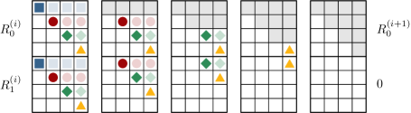
Fig. 3: A parallel “peel-off” procedure on $4\times 4$ matrices, in $4$ stages. The rows with the same symbol are transformed in a stage independently of each other by the Givens rotations computed from the dark-colored diagonal elements. The final elements of $R_{0}^{(i+1)}$ are fully shaded.

Each remaining chunk of $\begin{bmatrix}G_{\mathsf{p}}&G_{\mathsf{q}}\end{bmatrix}$ is loaded into $A_{1}^{(i)}$, factored as $A_{1}^{(i)}=Q_{1}^{(i)}R_{1}^{(i)}$, and combined with $R_{0}^{(i)}$ to obtain $R_{0}^{(i+1)}$. After the final $R_{\mathsf{p}\mathsf{q}}=R_{0}^{(n/32-1)}$ is formed, $V_{\mathsf{p}\mathsf{q}}^{\prime}$ is set to $I_{32}$.

Unfortunately, this approach is not recommendable when efficiency matters. For example, on matrices of order $3072$, the QR factorization is $12$–$15$ times slower than the Cholesky factorization, depending on the column norm computation algorithm.

4.3 The orthogonalization

In this phase, the inner pointwise Jacobi (H)SVD method is run on $R_{\mathsf{p}\mathsf{q}}$. A constant memory parameter $M_{\mathrm{s}}$, representing the maximal number of inner sweeps, decides whether the block-oriented ($M_{\mathrm{s}}=1$) or the full block variant ($M_{\mathrm{s}}>1$, usually $M_{\mathrm{s}}=30$) should be performed.

The inner p-strategy $\mathcal{S}_{32}^{\prime}$ is encoded into a constant memory lookup table $S_{32}^{\prime}$. In principle, $\mathcal{S}_{32}^{\prime}$ need not be of the same type of p-strategies as $\mathcal{S}_{\mathsf{b}}$. For example, $\mathcal{S}_{32}^{\prime}$ may be of the Brent and Luk type, and $\mathcal{S}_{\mathsf{b}}$ may be of the Matharam-Eberlein type, but usually a choice of the p-strategies is uniform, with only a single type for all levels.

In each p-step $s$ of an inner sweep $r$, the warp $y$ is assigned the pivot pair $(p,q)=S_{32}^{\prime}(r,s)[y]$, i.e., the pair of columns $\begin{bmatrix}g_{p}&g_{q}\end{bmatrix}$ of $R_{\mathsf{p}\mathsf{q}}$, and the pair of columns $\begin{bmatrix}v_{p}&v_{q}\end{bmatrix}$ of $V_{\mathsf{p}\mathsf{q}}^{\prime}$. Then, the following subphases are executed:

1. The $2\times 2$ pivot matrix $\widehat{H}_{pq}$ from (3) is computed. As explained in Subsection 4.3.1, three dot products (for $h_{pq}$, $h_{pp}$, and $h_{qq}$) are needed when the rotation formulas from [13] are not used. The elements $g_{p}[x]$, $g_{q}[x]$, $v_{p}[x]$, and $v_{q}[x]$ are preloaded into registers of a thread with lane ID $x$, so, e.g., $V_{\mathsf{p}\mathsf{q}}^{\prime}$ may be overwritten as a scratch space for warp-level reductions on Fermi GPUs.

2. The relative orthogonality criterion for $g_{p}$ and $g_{q}$ is fulfilled if

   $$|h_{pq}|<c(\varepsilon)\sqrt{h_{pp}}\sqrt{h_{qq}}=c(\varepsilon)\|g_{p}\|_{2}\|g_{q}\|_{2},$$

   where $c(\varepsilon)=\varepsilon\sqrt{\hat{n}}$, and $\hat{n}$ is the matrix order (here, $\hat{n}=32$). If $g_{p}$ and $g_{q}$ are relatively orthogonal, then set an indicator $\rho_{s}$, that determines whether a rotation should be applied, to $\rho_{s}=0$, else set $\rho_{s}=1$. Note that $\rho_{s}$ is a per-thread variable, but has the same value across a warp.

3. Let $a_{s}$ be a thread-block-wide number of warps about to perform the rotations. A warp has $32$ threads, so $a_{s}=(\Sigma\rho_{s})/32$, where the sum ranges over all threads in the thread block. Compute $a_{s}$ as $\mathop{\text{{\_\_syncthreads\_count}}}(\rho_{s})/32$. Since the pointwise Jacobi process stops if no rotations occurred in a sweep, we have to increase a per-sweep counter of rotations, $A_{r}$, by $a_{s}$. The counters $a_{s}$ and $A_{r}$ are kept per thread, but have the same value in the thread block.

4. Let the pivot indices $p$ and $q$ correspond to the columns $k$ and $\ell$, respectively, of the input factor $G$. If $k\leq n_{+}<\ell$, then compute the transformation $\widehat{V}_{pq}$ from (4) as a hyperbolic rotation (14), else as a trigonometric one (13), according to Subsection 4.3.1. If $\operatorname{cs}\varphi\neq 1$, then set $\rho_{s}^{\prime}=1$ (a proper rotation), else leave $\rho_{s}^{\prime}=0$ to indicate that the rotation is nearly identity. If $\rho_{s}$ was $0$, just determine if the rotation would be a trigonometric or a hyperbolic one, instead of computing it.

5. If the rotation is trigonometric, find the new diagonal elements, $h_{pp}^{\prime}$ and $h_{qq}^{\prime}$,

   $$h_{pp}^{\prime}=\operatorname{\mathtt{fma}}(\tan\varphi,h_{pq},h_{pp}),\quad h_{qq}^{\prime}=\operatorname{\mathtt{fma}}(-\tan\varphi,h_{pq},h_{qq}).$$

   If $\rho_{s}=0$ (i.e., $\widehat{V}_{pq}$ is the identity), take $h_{pp}^{\prime}=h_{pp}$ and $h_{qq}^{\prime}=h_{qq}$. To keep the eigenvalues sorted non-increasingly [21], if $h_{pp}^{\prime}<h_{qq}^{\prime}$ when $\ell\leq n_{+}$, or $h_{pp}^{\prime}>h_{qq}^{\prime}$ when $k>n_{+}$, set $P_{2}=\left[\begin{smallmatrix}0&1\\ 1&0\end{smallmatrix}\right]$, else $P_{2}=I_{2}$. Define

   $$\widehat{V}_{pq}^{\prime}=\widehat{V}_{pq}P_{2}.$$

   The eigenvalue order tends to stabilize eventually, thus no swapping is usually needed in the last few sweeps [28, 29]. If the rotation is hyperbolic, to keep $J$ partitioned, set $\widehat{V}_{pq}^{\prime}=\widehat{V}_{pq}$ (there is no sorting, and the new diagonal elements are not needed). An unpartitioned $J$ could lead to a slower convergence [35].

6. Apply, per thread, $\widehat{V}_{pq}^{\prime}$ to $\begin{bmatrix}g_{p}[x]&g_{q}[x]\end{bmatrix}$ and $\begin{bmatrix}v_{p}[x]&v_{q}[x]\end{bmatrix}$ from the right, and store the new values into shared memory.

7. Compute $b_{s}=(\Sigma\rho_{s}^{\prime})/32$, similarly to subphase $3$, and increase a per-sweep counter of proper rotations $B_{r}$ by $b_{s}$. This concludes the actions of one p-step.

After the sweep $r$ finishes, update $B$, the total number of proper rotations in the thread block, by $B_{r}$. If no more sweeps follow, i.e., if $A_{r}=0$ (no rotations have been performed in the last sweep), or $r=M_{\mathrm{s}}$ (the maximal number of sweeps is reached), the thread $[0,0]$ atomically adds $B$ to the global rotation counter $\mathsf{B}$, mapped from the CPU memory.

In $\mathsf{B}$ the number of rotations from all thread blocks is accumulated. Note that $\mathsf{B}$ is accessible from both the CPU and the GPU, and is the sole quantum of information needed to stop the global Jacobi process. More details about a GPU-wide stopping criterion can be found in Subsection 4.5. This ends orthogonalize phase.

4.3.1 The Jacobi rotations

The numerically stable, state-of-the-art procedure of computing the trigonometric Jacobi rotations is described in [13]. The procedure relies on computing the column norms reliably, as described in Appendix A.

The rest of the computation from [13] is straightforward to implement. Since the entire shared memory per thread block is occupied, storing and updating the column scales, as in [1], is not possible without changing the shared memory configuration and reducing the L1 cache. The memory traffic that would thus be incurred overweights the two additional multiplications by a cosine per GPU thread. Therefore, rotations in the following form ($\operatorname{\mathtt{fma}}$ followed by a multiplication, if $\cos\varphi\neq 1$) are chosen,

(13) $$\begin{bmatrix}g_{p}^{\prime}&g_{q}^{\prime}\end{bmatrix}=\cos\varphi\begin{bmatrix}g_{p}&g_{q}\end{bmatrix}\begin{bmatrix}\hphantom{-}1&\tan\varphi\\ -\tan\varphi&1\end{bmatrix}.$$

The hyperbolic rotations may be computed similarly to the trigonometric ones, by adapting the ideas from [13], in the form

(14) $$\begin{bmatrix}g_{p}^{\prime}&g_{q}^{\prime}\end{bmatrix}=\cosh\varphi\begin{bmatrix}g_{p}&g_{q}\end{bmatrix}\begin{bmatrix}1&\tanh\varphi\\ \tanh\varphi&1\end{bmatrix}.$$

Let DDRJAC be a procedure that computes, as in [13], the trigonometric rotations in form (13) from the column norms it obtains by calling DRDSSQ (see Appendix A). On a Fermi GPU (matrix order $6144$), DDRJAC is only $14$% slower than a simple procedure we discuss in the sequel. However, the protection from the input columns of too large (or too small) norm that DDRJAC offers has to be complemented by the QR factorization at all blocking levels, which is extremely expensive.

Assume instead that the Gram matrix formation, the ordinary scalar products, and the induced norm computations never overflow. By using only correctly rounded arithmetic, $\cos\varphi$ and $\tan\varphi$ of (13), or $\cosh\varphi$ and $\tanh\varphi$ of (14), may be computed as in (15)–(18) (an adapted version of the Rutishauser formulas [32]):

(15) $$h=h_{qq}-\mathfrak{t}\cdot h_{pp};\quad\operatorname{ct}2\varphi=\mathfrak{t}\cdot\frac{h}{2h_{pq}};$$

(16) $$|\operatorname{ct}\varphi|=|\operatorname{ct}2\varphi|+\sqrt{\operatorname{\mathtt{fma}}(\operatorname{ct}2\varphi,\operatorname{ct}2\varphi,\mathfrak{t})};$$

(17) $$\operatorname{tn}\varphi=\operatorname{sgn}(\operatorname{ct}2\varphi)\cdot\operatorname{\mathtt{rcp}}(|\operatorname{ct}\varphi|);$$

(18) $$\operatorname{cs}_{1}\varphi=\operatorname{\mathtt{rcp}}(\sqrt{\operatorname{\mathtt{fma}}(\mathfrak{t}\cdot\operatorname{tn}\varphi,\operatorname{tn}\varphi,1)});\quad\operatorname{cs}_{2}\varphi=\frac{|\operatorname{ct}\varphi|}{\sqrt{\operatorname{\mathtt{fma}}(|\operatorname{ct}\varphi|,|\operatorname{ct}\varphi|,\mathfrak{t})}}.$$

Formulas (15)–(18), for $\mathfrak{t}=1$, produce the parameters of a trigonometric rotation ($\operatorname{ct}=\cot$, $\operatorname{tn}=\tan$, $\operatorname{cs}=\cos$), and for $\mathfrak{t}=-1$, of a hyperbolic rotation ($\operatorname{ct}=\coth$, $\operatorname{tn}=\tanh$, $\operatorname{cs}=\cosh$). If, numerically, $|\coth 2\varphi|=1$, it is substituted by $5/4$ (see [41]).

If $|\cot 2\varphi|<\sqrt{\varepsilon}$, then $\sqrt{\operatorname{\mathtt{fma}}(\cot 2\varphi,\cot 2\varphi,1)}=1$, and (16) in the trigonometric case simplifies to $|\cot\varphi|=|\cot 2\varphi|+1$. If $|\operatorname{ct}2\varphi|\geq\sqrt{2/\varepsilon}$, then (barring an overflow) $\sqrt{\operatorname{\mathtt{fma}}(\operatorname{ct}2\varphi,\operatorname{ct}2\varphi,\mathfrak{t})}=|\operatorname{ct}2\varphi|$, with (16) and (18) simplifying to $|\operatorname{ct}\varphi|=2\cdot|\operatorname{ct}2\varphi|$ and $\operatorname{cs}\varphi=1$, respectively. These simplifications avoid taking square roots and a possible overflow of $\operatorname{ct}^{2}2\varphi$, at a price of at most $3$ floating-point comparisons. If $|\operatorname{ct}2\varphi|\leq\nu/4$, then $\operatorname{tn}$ is normalized.

In (18) there are two mathematically (but not numerically) equivalent expressions, $\operatorname{cs}_{1}\varphi$ and $\operatorname{cs}_{2}\varphi$, which compute the cosine. By a similar analysis as above, $|\operatorname{ct}\varphi|\geq\sqrt{2/\varepsilon}$ implies $\operatorname{cs}_{2}\varphi=1$, $\operatorname{tn}\varphi\leq\sqrt{\varepsilon/2}$, and therefore $\operatorname{cs}_{1}\varphi=1$. Testing that condition also avoids an overflow of $\operatorname{ct}^{2}\varphi$. Motivated by the preliminary results described in Appendix B, we have chosen the $\operatorname{cs}_{2}\varphi$ formula for our implementation.

4.4 The postmultiplication

This phase postmultiplies $\begin{bmatrix}G_{\mathsf{p}}&G_{\mathsf{q}}\end{bmatrix}$ and, optionally, $\begin{bmatrix}V_{\mathsf{p}}&V_{\mathsf{q}}\end{bmatrix}$ by $V_{\mathsf{p}\mathsf{q}}^{\prime}$ only if the rotation counter from orthogonalize is non-zero, i.e., if $V_{\mathsf{p}\mathsf{q}}^{\prime}\neq I_{32}$. Let $A_{\mathsf{p}\mathsf{q}}$ alias the first half of $G_{\mathsf{p}\mathsf{q}}$ (i.e., $R_{\mathsf{p}\mathsf{q}}$). The procedure, detailed in Alg. 4.2, is based on the Cannon parallel matrix multiplication algorithm [6].

Description : Input: $\begin{bmatrix}A_{\mathsf{p}}&A_{\mathsf{q}}\end{bmatrix},A\in\{G,V\}$. Output: $\begin{bmatrix}A_{\mathsf{p}}^{\prime}&A_{\mathsf{q}}^{\prime}\end{bmatrix}=\begin{bmatrix}A_{\mathsf{p}}&A_{\mathsf{q}}\end{bmatrix}V_{\mathsf{p}\mathsf{q}}^{\prime}$.

for $(i=x;\,i<n;\,i\mathop{{+}{=}}32)$ // multiply the next chunk of $\begin{bmatrix}A_{\mathsf{p}}&A_{\mathsf{q}}\end{bmatrix}$ by $V_{\mathsf{p}\mathsf{q}}^{\prime}$

      $A_{\mathsf{p}\mathsf{q}}[x,y]=A_{\mathsf{p}}[i,y];\quad A_{\mathsf{p}\mathsf{q}}[x,y^{\prime}]=A_{\mathsf{q}}[i,y]$;

        // load the RAM chunk into $A_{\mathsf{p}\mathsf{q}}$

       __syncthreads();

        // ensure the shared memory writes have taken effect

       $a_{xy}=a_{xy^{\prime}}=0$;

        // $\begin{bmatrix}A_{\mathsf{p}}^{\prime}&A_{\mathsf{q}}^{\prime}\end{bmatrix}$ elements kept in registers

       $j=(y+x)\bmod 32;\quad j^{\prime}=(y^{\prime}+x)\bmod 32$;

        // initial skew modulo $32$

       unrolled for $(k=0;\,k<32;\,{+}{+}k)$ // multiply-and-cyclic-shift

            $a_{xy}=\operatorname{\mathtt{fma}}(A_{\mathsf{p}\mathsf{q}}[x,j],V_{\mathsf{p}\mathsf{q}}^{\prime}[j,y],a_{xy})$;

              // update $A_{\mathsf{p}}^{\prime}[i,y]$

             $a_{xy^{\prime}}=\operatorname{\mathtt{fma}}(A_{\mathsf{p}\mathsf{q}}[x,j^{\prime}],V_{\mathsf{p}\mathsf{q}}^{\prime}[j^{\prime},y^{\prime}],a_{xy^{\prime}})$;

              // update $A_{\mathsf{q}}^{\prime}[i,y]$

             $j=(j+1)\bmod 32;\quad j^{\prime}=(j^{\prime}+1)\bmod 32$;

              // cyclic shift modulo $32$

            

       endfor

      __syncthreads();

        // ensure that $A_{\mathsf{p}\mathsf{q}}$ is free to be overwritten

       $A_{\mathsf{p}}^{\prime}[i,y]=a_{xy};\quad A_{\mathsf{q}}^{\prime}[i,y]=a_{xy^{\prime}}$;

        // store the product in the RAM chunk

      

endfor

Algorithm 4.2 Device function for Cannon-like postmultiplication by $V_{\mathsf{p}\mathsf{q}}^{\prime}$.

Finally, Fig. 4 summarizes the entire pStep kernel, from a perspective of the shared memory state transitions per thread block. The GPU RAM is accessed by one read (when no rotations occur), or by two reads and one write per element of $G$ (and, optionally, at most one read and write per element of $V$), with all operations fully coalesced. The only additional global memory traffic are the atomic reductions necessary for the convergence criterion in orthogonalize.

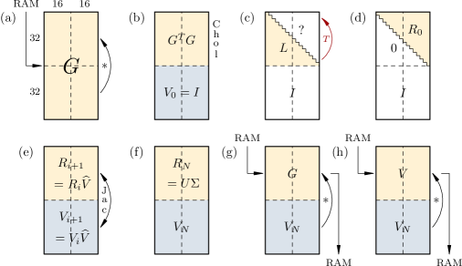
Fig. 4: An overview of pStep kernel per thread block, the full block variant. Each subfigure depicts the state of the shared memory, the computation subphase performed, and the data transfer in or out of the GPU RAM. Subfigures (a)–(d) illustrate factorize with the Cholesky factorization, (e) and (f) belong to orthogonalize, and (g) and (h) to postmultiply phase.

4.5 A GPU-wide convergence criterion

Contrary to the pointwise Jacobi algorithm, which is considered to converge when no rotations have been performed in a sweep, stopping of the block algorithms for large inputs is more complicated than observing no rotations in a block sweep. There has to be an additional, more relaxed stopping criterion at the block level (motivated in the sequel), while keeping the one at the inner ($32\times 32$) level unchanged.

The columns addressed by a pivot block-pair should be relatively orthogonal after completion of the pStep call in the full-block variant, but instead they may have departed from orthogonality, because (see [21, 37])

1. the accumulated rotations are not perfectly ($J$-)orthogonal, and

2. the postmultiplication introduces rounding errors.

Independently from that, in all variants, even the numerically orthogonal columns, when subjected to factorize (and its rounding errors), may result in the shortened ones that fail the relative orthogonality criterion.

If an orthogonality failure results from the first two causes, the ensuing rotations might be justified. However, if the failure is caused only by the rounding errors of the factorization process, the spurious rotations needlessly spoil the overall convergence.

To overcome this problem, we devised a simple heuristics to avoid excessive block sweeps with just a few rotations. We expect these rotations not to be proper, i.e., to have very small angles. Let $\mathsf{B}$ be a counter in the CPU RAM, mapped to the GPU RAM. The counter is reset at the beginning of each block sweep, and is updated from the pStep calls as described in Subsection 4.3. At the end of a block sweep, $\mathsf{B}$ contains the total number of proper rotations in that sweep. If $\mathsf{B}=0$, or the maximal number of block sweeps has been reached without convergence, the process stops.

This heuristics may skip over a relatively small number of legitimate rotations, but nevertheless produces reasonable relative errors in the computed singular values (see Section 6). A reliable way of telling (or avoiding) the exact cause of the orthogonality failures is strongly needed in that respect.

5 A multi-GPU algorithm

In this Section we apply the same blocking principles one level up the hierarchy, to the case of multiple GPUs. As a proof-of-concept, the algorithm is developed on a $4$-GPU Tesla S2050 system, and implemented as a single CPU process with $4$ threads, where the thread $0,\ldots,3$ controls the same-numbered GPU. Were the GPUs connected to multiple machines, on each machine the setup could be similar, with a CPU process and an adequate number of threads. Multiple processes on different machines could communicate via the CUDA-optimized MPI subsystem. Except replacing the inter-GPU communication APIs, the algorithm would stay the same.

Each of $\mathsf{g}$ GPUs holds two block-columns addressed by a pivot block-pair with a total of $\mathsf{n}=n/\mathsf{g}$ columns. For simplicity, we assume $n\bmod\mathsf{g}=0$. After an outer block step, a single block-column on a GPU $i$ is sent to a GPU $j$, and replaced by the one received from a GPU $k$, where $j$ may or may not be equal to $k$, according to a block-column mapping $S_{2\mathsf{g}}^{\prime\prime}$. For the outer p-strategy $\mathcal{S}_{2\mathsf{g}}^{\prime\prime}$, a block-column mapping has to be chosen such that the communication rules implied by the mapping are (nearly) optimal for the given network topology.

For example, in our test system with $\mathsf{g}=4$, a GPU $i$ communicates with a GPU $j$, $j=i\operatorname{xor}1$, faster than with the others. We maximized the amount of fast exchanges within an outer block sweep for $\text{\reflectbox{$\mathcal{R}$}}_{8}^{\parallel}$ (equivalent to Mantharam–Eberlein BR on a two-dimensional hypercube) to $3$, by choosing which pivot block-pair is assigned to which GPU in each block step. The result is a block-column mapping shown in Fig. 5.

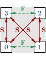
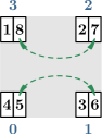
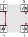
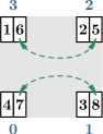
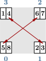
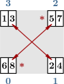
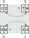
Fig. 5: The block-column mapping in a single block sweep of a p-strategy equivalent to Mantharam–Eberlein BR to GPUs $0,\ldots,3$. The fast (F) communications for column exchanges between GPU peers are denoted by dashed curves, and the slow (S) exchanges by solid lines. Two-speed communication is defined on the top left subfigure. The (logical) column swaps needed to maintain $p<q$ are shown by an asterisk.

Besides the two outer block-columns of $G$ (and, optionally, $V$), stored in $G_{A}$ and $V_{A}$ regions of the GPU RAM, respectively, an additional buffer space of the same size, $G_{B}$ and $V_{B}$, has to be allocated to facilitate the BLAS 3-style matrix multiplications and the full-duplex asynchronous communication between GPUs. Also, for the shortening and the single-GPU Jacobi phases, two $\mathsf{n}\times\mathsf{n}$ matrices, $X$ and $Y$, are needed. With a small auxiliary space AUX for the final singular value extraction, the total memory requirements are at most $m\times 5\mathsf{n}$ double elements per GPU.

In an outer block step the following operations are performed (see Fig. 6):

1. form the Gram matrix $G_{A}^{T}G_{A}$ in $X$ by cublasDsyrk;

2. factorize $G_{A}^{T}G_{A}=R^{T}R$ by the Cholesky factorization (we have chosen hybrid MAGMA’s dpotrf_gpu, and this is the only place where a CPU is used for computation, which may be circumvented by a GPU-only implementation);

3. case (acc.): if accumulation of the product $\widehat{V}$ of the Jacobi rotations is desired, call a full SVD single-GPU Jacobi variant (the full block, the block-oriented, or a hybrid one) from Section 4 on $X$, storing $\widehat{V}$ in $Y$; else

4. case (solve): copy $R$ from $X$ to $Y$, call a partial SVD single-GPU Jacobi variant on $Y$, and solve the triangular linear system $R\widehat{V}=\widehat{U}\widehat{\Sigma}$ for $\widehat{V}$ by cublasDtrsm, with the original $R$ in $X$ and $\widehat{V}$ overwriting $\widehat{U}\widehat{\Sigma}$ in $Y$;

5. postmultiply $G_{A}$ and $V_{A}$ by $\widehat{V}$, using two cublasDgemm calls running in their own CUDA streams, and store the updated block-columns in $G_{B}$ and $V_{B}$;

6. ensure that all GPUs have completed the local updates by a device-wide synchronization (cudaDeviceSynchronize), followed by a process-wide thread synchronization (wait on a common barrier), and a suitable MPI collective operation (e.g., MPI_Barrier) in the multi-process case;

7. start, via CUDA streams, the asynchronous sends of one block-column from $G_{B}$ and the corresponding one from $V_{B}$ to another GPU, and start the asynchronous copies of the other column of $G_{B}$ and the corresponding one of $V_{B}$ to either the first or the second block-column of $G_{A}$ and $V_{A}$, according to the block-column mapping rules for transition to the subsequent block step;

8. wait for the outstanding asynchronous operations to finish by the same synchronization procedure as in (4), after which a block step is completed.

At the end of an outer block sweep, the threads (and processes, where applicable) ${+}$-reduce their local counters $\mathsf{B}_{i}$ of proper rotations (cf. Subsection 4.5) to the system-wide number $\sum_{i}\mathsf{B}_{i}$ of proper rotations performed in all block steps in that sweep. If the result is $0$, or the limit on the number block sweeps has been reached, the iteration stops and the final singular values are extracted.

The full block variant of phases (2a) and (2b) usually has $30$ sweeps limit for both the inner blocking and the pointwise, shared-memory Jacobi level. The block-oriented variant has both limits set to $1$. Between them many hybrid variants may be interpolated.

Observe that phase (4) forces all GPUs to wait for the slowest one, in terms of the execution of phase (2a) or (2b). The full block variant exhibits the largest differences in running times between GPUs, depending on how orthogonal the block-columns are in the current block step. Although the full block variant is the fastest choice for a single-GPU algorithm (see Section 6), it may be up to $35$% slower in a multi-GPU algorithm than the block-oriented variant, which has a predictable, balanced running time on all GPUs.

A reasonable hybrid variant might try to keep the running times balanced. A CPU thread that first completes the full block variant of (2a) or (2b) informs immediately other threads, before proceeding to phase (4). The other threads then stop their inner block sweeps loops in (2a) or (2b) when the running iteration is finished.

The wall execution times of such an approach may be even lower than the block-oriented variant, but on the average are $10$% higher. Moreover, both the full block and its hybrid variant induce the larger relative errors in $\Sigma$ than the block-oriented variant. Such effect may be partially explained, as in Section 6, by the same reasons valid for the single-GPU case (more rotations applied), but the larger differences in the multi-GPU case require further attention. We have therefore presented the numerical tests for the block-oriented multi-GPU variant only.

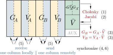
Fig. 6: Schematics of a GPU’s memory organization and the outer block step phases. Operations with the same number may be performed concurrently, in streams, if the hardware allows that.

6 Numerical testing

In this section we define the testing data, describe the hardware, and present the speed and accuracy results for both the single-GPU and the multi-GPU implementations. By these results we also confirm our p-strategies ($\text{\reflectbox{$\mathcal{R}$}}^{\parallel}$ and $\text{\reflectbox{$\mathcal{C}$}}^{\parallel}$) from Section 3 as a reliable choice for implementing the fast Jacobi algorithms on the various parallel architectures.

Let $\mathtt{norm}$ and $\mathtt{unif}$ be the double precision pseudorandom number generators, such that $\mathop{\mathtt{norm}}(\mu,\sigma)$ returns the non-zero samples from normal distribution $\mathop{\mathcal{N}}(\mu,\sigma)$, and $\mathop{\mathtt{unif}}(S)$ returns the samples from the continuous uniform distribution $\mathcal{U}$ over $S$. We have generated the following pseudorandom spectra, for $k=1,\ldots,16$:

1. $\Lambda_{k}^{(1)}(1{:}16)=0.5$; $\Lambda_{k}^{(1)}(17{:}1024k)=\mathop{\mathtt{norm}}(0,0.1)$,

2. $\Lambda_{k}^{(2)}=1+\Lambda_{k}^{(1)}$ (verified to be greater than zero),

3. $\Lambda_{k}^{(3)}(1{:}1024k)=\pm\mathop{\mathtt{unif}}(\langle 10^{-7},10k\rangle)$, where a positive or a negative sign for each $\Lambda_{k}^{(3)}(i)$ is chosen independently for $1\leq i\leq 1024k$ with equal probability,

4. $\Lambda_{k}^{(4)}(1{:}1024k)=\mathop{\mathtt{unif}}(\langle 10^{-7},10k\rangle)$.

These arrays have been casted to the Fortran’s quadruple precision type, and denoted by $\mathbf{\Lambda}_{k}^{(1)}$ to $\mathbf{\Lambda}_{k}^{(4)}$. By a modified LAPACK xLAGSY routine, working in quadruple precision, a set of symmetric matrices $\mathbf{A}_{k}^{(j)}=\mathbf{U}_{k}^{(j)}\mathbf{\Lambda}_{k}^{(j)}[\mathbf{U}_{k}^{(j)}]^{T}$ has been generated, for $j=1,\ldots,4$, by pre- and post-multiplying $\mathbf{\Lambda}_{k}^{(j)}$ with a product $\mathbf{U}_{k}^{(j)}$ of the random Householder reflectors. The matrices $\mathbf{A}_{k}^{(j)}$ have then been factored by the symmetric indefinite factorization with the complete pivoting [38] in quadruple precision:

$$P_{k}^{(j)}\mathbf{A}_{k}^{(j)}[P_{k}^{(j)}]^{T}=\widehat{\mathbf{G}}_{k}^{(j)}\widetilde{P}_{k}^{(j)}[\widetilde{P}_{k}^{(j)}]^{T}\widehat{J}_{k}^{(j)}\widetilde{P}_{k}^{(j)}[\widetilde{P}_{k}^{(j)}]^{T}[\widehat{\mathbf{G}}_{k}^{(j)}]^{T}=\mathbf{G}_{k}^{(j)}J_{k}^{(j)}[\mathbf{G}_{k}^{(j)}]^{T}.$$

The inner permutation $\widetilde{P}_{k}^{(j)}$ brings $\widehat{J}_{k}^{(j)}$ into $J_{k}^{(j)}=\mathop{\operator@font diag}\nolimits(I,-I)$ form. For $j\in\{2,4\}$ the symmetric indefinite factorization is equivalent to the Cholesky factorization with diagonal pivoting ($J_{k}^{(j)}=I$). Finally, $\mathbf{G}_{k}^{(j)}$ have been rounded back to double precision, and stored as the input factors $G_{k}^{(j)}$, along with $\Lambda_{k}^{(j)}$ and $J_{k}^{(j)}$.

Since one of the important applications of the (H)SVD is the eigensystem computation of the symmetric (in)definite matrices, the procedure just described has been designed to minimize, as much as it is computationally feasible, the effect of the rounding errors in the factorization part. We have, therefore, measured the relative errors of the computed $\Sigma^{2}J$ (from $G=U\Sigma V^{T}$) vs. the given $\Lambda_{k}^{(j)}$ (with the elements denoted $\lambda_{i}$, for $1\leq i\leq n$), i.e.,

(19) $$\max_{i=1,\ldots,n}\frac{|\operatorname{\mathit{f\mkern-2.0mu\ell}}(\sigma_{i})^{2}j_{i}-\lambda_{i}|}{|\lambda_{i}|}.$$

It may be more natural and reliable to compute the (H)SVD of $G_{k}^{(j)}$ in quadruple precision and compare the obtained singular values with the ones produced by the double precision algorithms. For an extremely badly conditioned $\mathbf{A}$, $\sqrt{|\Lambda|}$ may not approximate the singular values of $G$ well; e.g., if by the same procedure as above, $\mathbf{A}$ (definite or indefinite) is generated, with $n=4096$ and $\kappa_{2}(\mathbf{A})\geq 10^{24}$, the resulting $G$ may have the singular values (found by the quadruple Jacobi algorithm) differing in at least $4$–$5$ least significant double precision digits from the prescribed singular values $\sqrt{|\Lambda|}$. However, for a larger $n$, the quadruple precision SVD computation is infeasible. We have therefore verified accuracy of our algorithms as in (19), but have generated the modestly conditioned test matrices to avoid the problems described.

The NVIDIA graphics testing hardware, with accompanying CPUs, consists of:

1. Tesla C2070 (Fermi) GPU and Intel Core i7–950 CPU ($4$ cores),

2. Tesla K20c (Kepler) GPU and Intel Core i7–4820K CPU ($4$ cores),

3. Tesla S2050 (Fermi) 4 GPUs and two Intel Xeon E5620 CPUs ($2\times 4$ cores).

The software used is CUDA 5.5 (nvcc and cuBLAS) under $64$-bit Windows and Linux, and MAGMA 1.3.0 (with sequential and parallel Intel MKL 11.1) under $64$-bit Linux.

As shown in Table 1, the sequential Jacobi algorithm DGESVJ, with the parallel MKL BLAS 1 operations, on machine C runs approximately $16$ times slower than a single-GPU (Fermi) algorithm for the large enough inputs.

Table 1: The ratio of the wall running times of DGESVJ on machine C vs. a single GPU (Fermi) for the Cholesky factors of the matrices of order $n=1024k$ with spectra $\Lambda_{k}^{(2)}$.

$k$	$\texttt{DGESVJ}/\text{\reflectbox{$\mathcal{R}$}}^{\parallel}$
1	05.57
2	08.61
3	11.75
4	11.83

$k$	$\texttt{DGESVJ}/\text{\reflectbox{$\mathcal{R}$}}^{\parallel}$
5	12.34
6	13.47
7	13.62
8	13.58

$k$	$\texttt{DGESVJ}/\text{\reflectbox{$\mathcal{R}$}}^{\parallel}$
09	14.89
10	15.45
11	15.62
12	16.14

$k$	$\texttt{DGESVJ}/\text{\reflectbox{$\mathcal{R}$}}^{\parallel}$
13	16.49
14	16.46
15	16.19
16	16.00

In Table 2 the differences in the execution times of the $\text{\reflectbox{$\mathcal{R}$}}^{\parallel}$ p-strategy on Fermi and Kepler are given. There are the three main reasons, outlined in Section 4, why the Kepler implementation is much faster than the Fermi one. In order of importance:

1. $8$-byte wide shared memory banks on Kepler vs. $4$-byte wide on Fermi—the profiler reports $99.8$% shared memory efficiency on Kepler vs. $49.8$% on Fermi,

2. warp shuffle reductions on Kepler (the warp-level reductions do not need the shared memory workspace), and

3. no register spillage on Kepler, due to the larger register file.

The other profiler metrics are also encouraging: the global memory loads and stores are more than $99$% efficient, and the warp execution efficiency on Fermi is about $96.5$%, which confirms that the presented algorithms are almost perfectly parallel.

Table 2: The wall running times (in seconds) of a Fermi ($F$) vs. a Kepler ($K$) GPU for the Cholesky factors of the matrices of order $n=1024k$ with spectra $\Lambda_{k}^{(2)}$, the full block variant.

$k$	$\text{Kepler}\,[\text{s}]$	$\text{Fermi}\,[\text{s}]$	$K/F\,[\text{\%}]$
1	001.413099	002.376498	59.5
2	007.206334	012.438532	57.9
3	022.980686	035.783290	64.2
4	046.357804	084.466500	54.9
5	095.828870	160.382859	59.8
6	154.643361	261.917934	59.0
7	246.114488	403.150779	61.0
8	346.689433	621.341377	55.8

$k$	$\text{Kepler}\,[\text{s}]$	$\text{Fermi}\,[\text{s}]$	$K/F\,[\text{\%}]$
09	0506.365598	0850.279539	59.6
10	0682.577101	1153.337956	59.2
11	0904.212224	1545.451594	58.5
12	1148.881987	1970.591570	58.3
13	1439.391787	2500.931105	57.6
14	1809.888207	3158.116986	57.3
15	2196.755474	3820.551746	57.5
16	2625.642659	4662.748709	56.3

Even though the instruction and thread block execution partial orders may vary across the hardware architectures, the presented algorithms are observably deterministic. Combined with a strong IEEE floating-point standard adherence of both the Fermi and the Kepler GPUs, that ensures the numerical results on one architecture are bitwise identical to the results on the other. This numerical reproducibility property should likewise be preserved on any future, standards-compliant hardware.

We proceed by showing that $\text{\reflectbox{$\mathcal{R}$}}^{\parallel}$ and $\text{\reflectbox{$\mathcal{C}$}}^{\parallel}$ p-strategies are superior in terms of speed to $\mathcal{R}^{\parallel}$, $\mathcal{C}^{\parallel}$, the Brent and Luk ($\mathcal{B}$), and modified modulus ($\mathcal{M}$) strategies, in both the definite and the indefinite case. By abuse of notation, we write $\text{\reflectbox{$\mathcal{R}$}}_{b}^{\parallel}$ for the block-oriented variant (otherwise, we measure the full block variant), and $\text{\reflectbox{$\mathcal{R}$}}_{4b}^{\parallel}$ for its $4$-GPU implementation. Fig. 7 depicts the wall time ratios of the other strategies vs. $\text{\reflectbox{$\mathcal{R}$}}^{\parallel}$. Except $\mathcal{B}$ and $\text{\reflectbox{$\mathcal{C}$}}^{\parallel}$, the other strategies are consistently about $14$–$21$% slower than $\text{\reflectbox{$\mathcal{R}$}}^{\parallel}$, while $\text{\reflectbox{$\mathcal{C}$}}^{\parallel}$ is almost equally fast as $\text{\reflectbox{$\mathcal{R}$}}^{\parallel}$. Therefore, in the sequel we have timed only $\text{\reflectbox{$\mathcal{R}$}}^{\parallel}$.

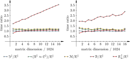
Fig. 7: The wall time ratio of the various parallel strategies on a single GPU (Fermi). The test spectra for the left graph are $\Lambda_{k}^{(2)}$, and for the right graph are $\Lambda_{k}^{(1)}$.

The standard counter-example that shows nonconvergence of the Jacobi method under the Brent and Luk strategy for matrices of even orders (first constructed by Hansen in [19], and later used in [26]), is actually not a counter-example in the usual diagonalization procedure which skips the rotations with the very small angles, because there is no need for diagonalization of an already diagonal matrix of order $2$. On the contrary, the standard algorithm will diagonalize this matrix in only one (second) step of the first sweep.

However, this still does not mean that no serious issues exist regarding convergence of the Jacobi method under $\mathcal{B}$. Fig. 7 indicates that a further investigation into the causes of the extremely slow convergence (approaching $30$ block sweeps) under $\mathcal{B}$ may be justified.

The block-oriented variant has more block sweeps and, while slightly faster for the smaller matrices, is about $7$% slower for the larger matrices than the full block variant. It may be more accurate in certain cases (see Fig. 8), due to the considerably smaller total number of the rotations performed, as shown in Table 3. The strategies $\mathcal{M}$ and $\mathcal{B}$ are far less accurate than the new p-strategies.

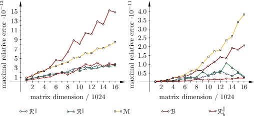
Fig. 8: The relative accuracy of the various parallel strategies on a single GPU. The test spectra for the left graph are $\Lambda_{k}^{(2)}$, and for the right graph are $\Lambda_{k}^{(1)}$.

Table 3: The number of block sweeps and the average ratios (with small variance) of the total number of rotations of the full block vs. the block-oriented variant, per $4$ spectrum types on a single GPU.

Spectrum type	1	2	3	4
average ratio of the number of rotations $\text{\reflectbox{$\mathcal{R}$}}^{\parallel}/\text{\reflectbox{$\mathcal{R}$}}_{b}^{\parallel}$	2.29	2.10	2.30	2.08
range of the number of block sweeps $\text{\reflectbox{$\mathcal{R}$}}^{\parallel}$	08–12	8–90	8–11	7–90
range of the number of block sweeps $\text{\reflectbox{$\mathcal{R}$}}_{b}^{\parallel}$	10–14	9–12	9–14	9–12

MAGMA’s dgesvd routine has been tested with the sequential (seq.) and the parallel (par.) ($4$ threads) MKL library on machine A. The relative accuracy is identical in both cases. Compared with the single-GPU Fermi algorithm, MAGMA (seq.) is $1.5$–$3$ times slower, and MAGMA (par.) is up to $2$ times faster. On the other hand, MAGMA (par.) is, on average, $30$%, and for the larger matrix sizes, more than $45$% slower than the block-oriented $4$-GPU Fermi (solve) implementation. The (acc.) implementation is about $35$% slower than (solve) (see Fig. 9), and only marginally more accurate (see Fig. 10). For the matrix orders of at least $4096$, the fastest Jacobi implementation on $4$ GPUs is about $2.7$ times faster than the fastest one on $1$ GPU.

MAGMA’s accuracy is comparable to a single-GPU algorithm for the well-conditioned test matrices, and better than a multi-GPU algorithm, but in the (separately tested) case of matrices with badly scaled columns ($\kappa_{2}\approx 10^{12}$), the relative errors of MAGMA could be more than $20$ times worse than the Jacobi ones.

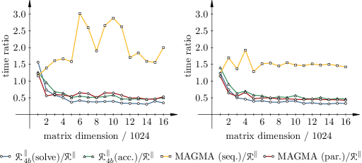
Fig. 9: The wall time ratio of the block-oriented $4$-GPU Fermi implementations and MAGMA vs. a single GPU. The test spectra for the left graph are $\Lambda_{k}^{(2)}$, and for the right graph are $\Lambda_{k}^{(4)}$.

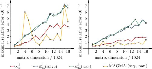
Fig. 10: The relative accuracy of the block-oriented $1$- and $4$-GPU Fermi implementations and MAGMA. The test spectra for the left graph are $\Lambda_{k}^{(2)}$, and for the right graph are $\Lambda_{k}^{(4)}$.

Unlike MAGMA, the Jacobi GPU algorithms are perfectly scalable to an arbitrary number of GPUs, when the matrix order is a growing function of the number of assigned GPUs. That makes the Jacobi-type algorithms readily applicable on the contemporary large-scale parallel computing machinery, which needs to leverage the potential of a substantial amount of numerical accelerators.

Conclusions

In this paper we have developed a set of new parallel Jacobi strategies, both faster and more accurate than the widely used ones. The new strategies may be seen as the generalizations of the Mantharam–Eberlein block-recursive strategy [27] to all even matrix orders. These new strategies are combined with the multi-level blocking and parallelization techniques explored in [20, 21, 37, 36, 29], to deliver the Jacobi-type (H)SVD algorithms for the graphics processing unit(s), competitive with the leading hybrid (CPU $\!+\!$ GPU) alternatives, like MAGMA. The new algorithms are carefully designed to use a CPU primarily as a controlling unit. To this end, a collection of the auxiliary shared-memory routines for the concurrent formation of the Gram matrices, the Cholesky and QR factorizations, and the numerically robust vector $2$-norm computations are proposed. The numerical results confirm that in the massively parallel GPU case the Jacobi-type methods retain all the known advantages [15, 16], while exhibiting noteworthy speed.

Appendix A Parallel norm computation

An essential prerequisite for computing the Householder reflectors and the Jacobi rotations [13] is obtaining the column norms (effectively, the sums of squares) reliably, avoiding the possible underflows and overflows of an ordinary scalar product. However, a strictly sequential nature of LAPACK’s DLASSQ is unsuitable for parallel processing. Therefore, we propose an alternate procedure, DRDSSQ, based on the parallel reduction concept.

Let $\mu$ be the smallest and $\nu$ the largest positive normalized floating-point number, $\varepsilon$ the maximal relative roundoff error ($\varepsilon=2^{-53}$ for double with rounding to nearest), $\gamma=1-\varepsilon$, $\delta=1+\varepsilon$, and $x$ a vector of length $n$, with no special values ($\pm\infty$, NaNs) for its components. A floating-point approximation of an exact quantity $\xi$ is denoted by $\operatorname{rn}(\xi)$, $\operatorname{ru}(\xi)$, or $\operatorname{rz}(\xi)$, for rounding to nearest, to $+\infty$, or to $0$, respectively.

Find $M\mathrel{\mathop{:}}=\max_{i}|x_{i}|$. If $M=0$, $x$ is a zero vector. Else, there exists the smallest non-zero $|x_{i}|$, which can be computed as $m\mathrel{\mathop{:}}=\min_{i}|x_{i}^{\prime}|$, where $x_{i}^{\prime}=x_{i}$ for $|x_{i}|>0$, and $x_{i}^{\prime}=\nu$ otherwise. Provided enough workspace for holding, or another technique for exchanging the partial results (such as the warp shuffle primitives of the Kepler GPU architecture), $M$ and $m$ could be found by a parallel min/max-reduction of $x$.

If the floating-point subnormals and infinity are supported, inexpensive, and safe to compute with (i.e., no exceptions are raised, or the non-stop exception handling is in effect), a sum of $x_{i}^{2}$ might also be computed. If the sum does not overflow, and a satisfactory accuracy is found to be maintained (e.g., the underflows could not have happened if $\operatorname{rn}(m^{2})\geq\mu$), DRDSSQ stops here.

Otherwise, note that the depth of a reduction tree for the summation of $x_{i}^{2}$ is $\lceil\lg n\rceil$, and at each tree level (the first one being level $0$) at most $\delta$ relative error is accumulated. Inductively, it follows that if, for some $s=2^{\ell}$,

$$2^{\lceil\lg n\rceil}(sM)^{2}\delta^{(1+\lceil\lg n\rceil)}\leq\nu,$$

then the sum of $(sx_{i})^{2}$ cannot overflow. Also, if $(sm)^{2}\gamma\geq\mu$, for some $s=2^{k}$, then no $(sx_{i})^{2}$ can underflow. If some $j$ could be substituted for both $k$ and $\ell$, it would define a scaling factor that simultaneously protects from the potential overflows and underflows. When the range of values of $x$ does not permit a single scaling, the independent scalings of too large and too small values of $x$ should be performed.

Such a scaling of $x_{i}$ by $s$ in the binary floating-point arithmetic introduces no rounding errors and amounts to a fast integer addition of the exponents of $x_{i}$ and $s$. Instead of the scale factors themselves, only their exponents need to be stored and manipulated as machine integers. For clarity, the scales remain written herein as the integer powers of $2$. A pair $(s,y)$ thus represents a number with the same precision as $y$, but with the exponent equal to a sum of the exponents of $s$ and $y$.

As motivated above, define the safe, inclusive bounds $\tilde{\mu}$ (lower) and $\hat{\nu}$ (upper) for the values of $x$ for which no overflow nor underflow can happen, as

$$\tilde{\mu}=\sqrt{\mu/\gamma},\quad\delta_{n}=2^{\lceil\lg n\rceil}\delta^{(1+\lceil\lg n\rceil)},\quad\hat{\nu}=\sqrt{\nu/\delta_{n}}.$$

Consider the following computations over a partition of the set of values of $x$:

• if $[m,M]\cap[\tilde{\mu},\hat{\nu}]\neq\emptyset$, set $s_{1}=1=2^{0}$ (no scaling needed), and compute

  $$\sigma_{1}^{2}=\sum_{i=1}^{n}\bar{x}_{i}^{2},\quad\bar{x}_{i}=\begin{cases}x_{i},&\tilde{\mu}\leq|x_{i}|\leq\hat{\nu},\\ 0,&\text{otherwise},\end{cases}$$

• if $M>\hat{\nu}$, take the largest $s$ such that $sM\leq\hat{\nu}$, denote it by $s_{2}$, and compute

  $$\sigma_{2}^{2}=\sum_{i=1}^{n}(s_{2}\hat{x}_{i})^{2},\quad\hat{x}_{i}=\begin{cases}x_{i},&|x_{i}|>\hat{\nu},\\ 0,&\text{otherwise},\end{cases}$$

• if $m<\tilde{\mu}$, take the smallest $s$ such that $sm\geq\tilde{\mu}$, denote it by $s_{0}$, and compute

  $$\sigma_{0}^{2}=\sum_{i=1}^{n}(s_{0}\tilde{x}_{i})^{2},\quad\tilde{x}_{i}=\begin{cases}x_{i},&|x_{i}|<\tilde{\mu},\\ 0,&\text{otherwise}.\end{cases}$$

From $m$, $M$, $\tilde{\mu}$, $\hat{\nu}$ it is known in advance which partial sums are necessarily $0$, and the procedure should be simplified accordingly. If, e.g., $m\geq\tilde{\mu}$, then $\sigma_{0}^{2}=0$.

A C/C++ implementation of finding $s_{0}=2^{k}$ or $s_{2}=2^{\ell}$ is remarkably simple. An expression y = frexp(x, &e) breaks $\mathtt{x}$ into $0.5\leq\mathtt{y}<1$ and $\mathtt{e}$ such that $2^{\mathtt{e}}\mathtt{y}=\mathtt{x}$. Let $\mathtt{f}=m$, $\mathtt{t}=\operatorname{ru}(\tilde{\mu})$, $\mathtt{j}=k$ for $s_{0}$, or $\mathtt{f}=M$, $\mathtt{t}=\operatorname{rz}(\hat{\nu})$, $\mathtt{j}=\ell$ for $s_{2}$. Also, let fy = frexp(f, &fe) and ty = frexp(t, &te). Then $\mathtt{j}$ is returned by a code fragment:

$$\verb|j = (f <= t) ? (te - fe) + (fy < ty) : (te - fe) - (fy > ty)|.$$

If there is more than one non-zero partial sum of squares, such $(s_{i}^{-2},\sigma_{i}^{2})$ are expressed in a “common form”, $(\breve{s}_{i}^{-2},\breve{\sigma}_{i}^{2})$, where $0.5\leq\breve{\sigma}_{i}^{2}<2$, and the scales’ exponents remain even. Let $(s_{i}^{-2},\sigma_{i}^{2})=(2^{j},2^{m}y)$, where $y$ is a significand of $\sigma_{i}^{2}$. Since $\sigma_{i}^{2}$ is normalized by construction, $1\leq y<2$. Define $m^{\prime}=-(m\bmod 2)$ and $j^{\prime}=j+m-m^{\prime}$. Then $m^{\prime}\in\{-1,0\}$, $j^{\prime}$ remains even, and $(\breve{s}_{i}^{-2},\breve{\sigma}_{i}^{2})=(2^{j^{\prime}},2^{m^{\prime}}y)$.

The common form makes ordering the pairs by their magnitudes equivalent to ordering them lexicographically. First, we find the two (out of at most three) partial sums which are the smallest by magnitude. We then add these partial sums together, such that the addend smaller by magnitude is rescaled to match the scale of the larger one. Let $(s_{+}^{-2},\sigma_{+}^{2})=(\breve{s}_{\leq}^{-2},\breve{\sigma}_{\leq}^{2})+(\breve{s}_{>}^{-2},\breve{\sigma}_{>}^{2})$, with $(\breve{s}_{\leq}^{-2},\breve{\sigma}_{\leq}^{2})\leq(\breve{s}_{>}^{-2},\breve{\sigma}_{>}^{2})$. Then $s_{+}^{-2}=\breve{s}_{>}^{-2}$, $s_{-}^{-2}=\breve{s}_{\leq}^{-2}/\breve{s}_{>}^{-2}$, and $\sigma_{+}^{2}=s_{-}^{-2}\breve{\sigma}_{\leq}^{2}+\breve{\sigma}_{>}^{2}$.

If one more addition is needed, $(s_{+}^{-2},\sigma_{+}^{2})$ has to be brought into the common form $(\breve{s}_{+}^{-2},\breve{\sigma}_{+}^{2})$, and summed with the remaining addend by the above procedure. However, both $(s_{2}^{-2},\sigma_{2}^{2})$ and $(s_{0}^{-2},\sigma_{0}^{2})$ have to be computed only when $n\tilde{\mu}^{2}\approx\varepsilon\hat{\nu}^{2}$. Such large $n$ seldom occurs. In either case, accuracy of the final result is maintained by accumulating the partial sums in the nondecreasing order of their magnitudes.

The result of DRDSSQ is $(s^{-2},\sigma^{2})$, and the norm of $x$ is $\|x\|_{2}=\sqrt{\sigma^{2}}/s$. If $\|x\|_{2}$ overflows or underflows for $x$ a column of $G$, the input factor should be initially rescaled (if possible). A procedure similar to DRDSSQ is implementable wherever the parallel reduction is a choice (e.g., with MPI_Allreduce operation).

By itself, DRDSSQ does not guarantee numerical reproducibility, if the underlying parallel reductions do not possess such guarantees. The ideas from [8] might be useful in that respect.

Appendix B A choice of the rotation formulas

In the block Jacobi algorithms, it is vital to preserve ($J$-)orthogonality of the accumulated $V$. In the hyperbolic case, the perturbation of the hyperbolic singular values also depends on the condition number of $V$ [21, Proposition 4.4]. A simple attempt would be to try to compute each rotation as ($J$-)orthogonal as possible, without sacrificing performance.

Departure from a single rotation’s ($J$-)orthogonality should be checked in a sufficiently high (e.g., $128$-bit quadruple) precision, as $d_{t}=|(\cos^{2}\varphi+\sin^{2}\varphi)-1|$, or as $d_{h}=|(\cosh\varphi-\sinh\varphi)(\cosh\varphi+\sinh\varphi)-1|$, with $\sin\varphi=\cos\varphi*\tan\varphi$, or $\sinh\varphi=\cosh\varphi*\tanh\varphi$. For each binary exponent $-53\leq\mathtt{e}\leq 53$ we generated, on a CPU, $2^{24}$ uniformly distributed pseudorandom $52$-bit integers $\mathtt{m}_{i}$, to form $|\operatorname{ct}2\varphi|_{i}$ with the exponent $\mathtt{e}$ and the non-implied bits of the significand equal to $\texttt{m}_{i}$. From $|\operatorname{ct}2\varphi|_{i}$ and (16)–(18) we computed $(\operatorname{tn}\varphi)_{i}$, $(\operatorname{cs}_{1}\varphi)_{i}$, and $(\operatorname{cs}_{2}\varphi)_{i}$ in double precision. In the Fortran’s quadruple arithmetic the corresponding $d_{t}$ and $d_{h}$ were then found and averaged, over all tested exponents. The results are summarized in Table 4.

Table 4: The average departures from ($J$-)orthogonality of the rotations given by (16)–(18).

trigonometric rotations		hyperbolic rotations
$d_{t}$ with $\cos_{1}\varphi$	$d_{t}$ with $\cos_{2}\varphi$	$d_{h}$ with $\cosh_{1}\varphi$	$d_{h}$ with $\cosh_{2}\varphi$
$8.270887\cdot 10^{-17}$	$8.335956\cdot 10^{-17}$	$7.575893\cdot 10^{-17}$	$6.586691\cdot 10^{-17}$

Table 4 indicates that $\cosh_{2}\varphi$ produces, on average, more $J$-orthogonal hyperbolic rotations than $\cosh_{1}\varphi$. In the trigonometric case it is the opposite, but with a far smaller difference. Orthogonality of the final $V$ was comparable in the tests for both trigonometric versions, often slightly better (by a fraction of the order of magnitude) using $\cos_{2}\varphi$. Therefore, $\operatorname{cs}_{2}\varphi$ formulas were chosen for a full-scale testing.

If $\operatorname{\mathtt{rsqrt}}(x)=1/\sqrt{x}$ were correctly rounded in CUDA, $\operatorname{cs}_{1}\varphi$ could be written as

(20) $$\operatorname{cs}_{1}^{\prime}\varphi=\operatorname{\mathtt{rsqrt}}(\operatorname{\mathtt{fma}}(\mathfrak{t}\cdot\operatorname{tn}\varphi,\operatorname{tn}\varphi,1)).$$

With (20) and a correctly rounded-to-nearest $\operatorname{\mathtt{rsqrt}}$ prototype CUDA implementation there was a further improvement of orthogonality of $V$. Although (20) has only one iterative operation ($\operatorname{\mathtt{rsqrt}}$) instead of two ($\operatorname{\mathtt{rcp}}$ and $\sqrt{x}$), and thus has a potential to be faster than (18), we omitted (20) from the testing due to a slowdown of about $1$% that we expect to vanish with the subsequent implementations of $\operatorname{\mathtt{rsqrt}}$.

It is still far from conclusive which formulas from (18) or (20), and for which ranges of $\operatorname{ct}2\varphi$, should be used. However, $\operatorname{cs}_{2}\varphi$ or $\operatorname{cs}_{1}^{\prime}\varphi$ formulas might be an alternative to the established $\operatorname{cs}_{1}\varphi$ ones. A deeper analysis is left for future work.

References

- [1] A. A. Anda and H. Park, Fast plane rotations with dynamic scaling, SIAM J. Matrix Anal. Appl., 15 (1994), pp. 162–174.
- [2] M. Anderson, G. Ballard, J. W. Demmel, and K. Keutzer, Communication-avoiding QR decomposition for GPUs, in Proceedings of the 25th IEEE International Parallel & Distributed Processing Symposium (IPDPS 2011), Anchorage, AK, USA, May 2011, pp. 48–58.
- [3] M. Bečka, G. Okša, and M. Vajteršic, Dynamic ordering for a parallel block–Jacobi SVD algorithm, Parallel Comput., 28 (2002), pp. 243–262.
- [4] R. P. Brent and F. T. Luk, The solution of singular-value and symmetric eigenvalue problems on multiprocessor arrays, SIAM J. Sci. Statist. Comput., 6 (1985), pp. 69–84.
- [5] R. P. Brent, F. T. Luk, and C. F. Van Loan, Computation of the singular value decomposition using mesh–connected processors, J. VLSI Comput. Syst., 1 (1985), pp. 242–270.
- [6] L. E. Cannon, A Cellular Computer to Implement the Kalman Filter Algorithm, PhD thesis, Montana State University, Bozeman, MT, USA, 1969.
- [7] NVIDIA Corp., CUDA C Programming Guide 5.5, July 2013.
- [8] J. Demmel and H. D. Nguyen, Fast reproducible floating-point summation, in Proceedings of the 21st IEEE Symposium on Computer Arithmetic (ARITH), Austin, TX, USA, April 2013, pp. 163–172.
- [9] J. W. Demmel, L. Grigori M. F. Hoemmen, and J. Langou, Communication–optimal parallel and sequential QR and LU factorizations, Technical Report UCB/EECS–2008–89, Electrical Engineering and Computer Sciences University of California at Berkeley, Aug. 2008.
- [10] , Communication–optimal parallel and sequential QR and LU factorizations, SIAM J. Sci. Comput., 34 (2012), pp. A206–A239.
- [11] J. W. Demmel and K. Veselić, Jacobi’s method is more accurate than QR, SIAM J. Matrix Anal. Appl., 13 (1992), pp. 1204–1245.
- [12] F. M. Dopico, P. Koev, and J. M. Molera, Implicit standard Jacobi gives high relative accuracy, Numer. Math., 113 (2009), pp. 519–553.
- [13] Z. Drmač, Implementation of Jacobi rotations for accurate singular value computation in floating point arithmetic, SIAM J. Sci. Comput., 18 (1997), pp. 1200–1222.
- [14] , A posteriori computation of the singular vectors in a preconditioned Jacobi SVD algorithm, IMA J. Numer. Anal., 19 (1999), pp. 191–213.
- [15] Z. Drmač and K. Veselić, New fast and accurate Jacobi SVD algorithm. I, SIAM J. Matrix Anal. Appl., 29 (2008), pp. 1322–1342.
- [16] , New fast and accurate Jacobi SVD algorithm. II, SIAM J. Matrix Anal. Appl., 29 (2008), pp. 1343–1362.
- [17] P. J. Eberlein, A one–sided Jacobi methods for parallel computation, SIAM J. Alg. Disc. Meth., 8 (1987), pp. 790–796.
- [18] G. R. Gao and S. J. Thomas, An optimal parallel Jacobi–like solution method for the singular value decomposition, in Proceedings of the 1988 International Conference on Parallel Processing, St. Charles, IL, USA, vol. 3, August 1988, pp. 47–53.
- [19] E. R. Hansen, On cyclic Jacobi methods, J. Soc. Indust. Appl. Math., 11 (1963), pp. 448–459.
- [20] V. Hari, S. Singer, and S. Singer, Block-oriented -Jacobi methods for Hermitian matrices, Linear Algebra Appl., 433 (2010), pp. 1491–1512.
- [21] , Full block -Jacobi method for Hermitian matrices, Linear Algebra Appl., 444 (2014), pp. 1–27.
- [22] M. R. Hestenes, Inversion of matrices by biorthonalization and related results, J. Soc. Indust. Appl. Math., 6 (1958), pp. 51–90.
- [23] D. S. Johnson, M. Yannakakis, and C. H. Papadimitriou, On generating all maximal independent sets, Inform. Process. Lett., 27 (1988), pp. 119–123.
- [24] S. Lahabar and P. J. Narayanan, Singular value decomposition on GPU using CUDA, in Proceedings of the 23rd IEEE International Symposium on Parallel & Distributed Processing (IPDPS 2009), Rome, Italy, no. 5161058, May 2009.
- [25] F. T. Luk and H. Park, On parallel Jacobi orderings, SIAM J. Sci. Statist. Comput., 10 (1989), pp. 18–26.
- [26] , A proof of convergence for two parallel Jacobi SVD algorithms, IEEE Trans. Comput., C–38 (1989), pp. 806–811.
- [27] M. Mantharam and P. J. Eberlein, Block recursive algorithm to generate Jacobi–sets, Parallel Comput., 19 (1993), pp. 481–496.
- [28] W. F. Mascarenhas, On the convergence of the Jacobi method for arbitrary orderings, SIAM J. Matrix Anal. Appl., 16 (1995), pp. 1197–1209.
- [29] V. Novaković and S. Singer, A GPU-based hyperbolic SVD algorithm, BIT, 51 (2011), pp. 1009–1030.
- [30] R. Onn, A. O. Steinhardt, and A. Bojanczyk, The hyperbolic singular value decomposition and applications, IEEE Trans. Signal Process., 39 (1991), pp. 1575–1588.
- [31] IEEE Task P754, IEEE 754-2008, Standard for Floating-Point Arithmetic, IEEE, New York, NY, USA, Aug. 2008.
- [32] H. Rutishauser, The Jacobi method for real symmetric matrices, Numer. Math., 9 (1966), pp. 1–10.
- [33] A. H. Sameh, On Jacobi and Jacobi–like algorithms for a parallel computer, Math. Comp., 25 (1971), pp. 579–590.
- [34] G. Shroff and R. S. Schreiber, On the convergence of the cyclic Jacobi method for parallel block orderings, SIAM J. Matrix Anal. Appl., 10 (1989), pp. 326–346.
- [35] S. Singer, S. Singer, V. Hari, K. Bokulić, D. Davidović, M. Jurešić, and A. Ušćumlić, Advances in speedup of the indefinite one-sided block Jacobi method, in AIP Conf. Proc. – Volume 936 Numerical Analysis and Applied Mathematics, T. E. Simos, G. Psihoyios, and Ch. Tsitouras, eds., Melville, New York, 2007, AIP, pp. 519–522.
- [36] S. Singer, S. Singer, V. Novaković, D. Davidović, K. Bokulić, and A. Ušćumlić, Three-level parallel -Jacobi algorithms for Hermitian matrices, Appl. Math. Comput., 218 (2012), pp. 5704–5725.
- [37] S. Singer, S. Singer, V. Novaković, A. Ušćumlić, and V. Dunjko, Novel modifications of parallel Jacobi algorithms, Numer. Alg., 59 (2012), pp. 1–27.
- [38] I. Slapničar, Componentwise analysis of direct factorization of real symmetric and Hermitian matrices, Linear Algebra Appl., 272 (1998), pp. 227–275.
- [39] S. Tomov, R. Nath, and J. Dongarra, Accelerating the reduction to upper Hessenberg, tridiagonal, and bidiagonal forms through hybrid GPU-based computing, Parallel Comput., 36 (2010), pp. 645–654.
- [40] C. F. Van Loan, The block Jacobi method for computing the singular value decomposition, in Computational and combinatorial methods in systems theory, Sel. Pap. 7th Int. Symp. Math. Theory Networks Syst., Stockholm 1985, 1986, pp. 245–255.
- [41] K. Veselić, A Jacobi eigenreduction algorithm for definite matrix pairs, Numer. Math., 64 (1993), pp. 241–269.
- [42] H. Zha, A note on the existence of the hyperbolic singular value decomposition, Linear Algebra Appl., 240 (1996), pp. 199–205.