Scattering theory of topological phases in discrete-time quantum walks

Abstract

One-dimensional discrete-time quantum walks show a rich spectrum of topological phases that have so far been exclusively analysed based on the Floquet operator in momentum space. In this work we introduce an alternative approach to topology which is based on the scattering matrix of a quantum walk, adapting concepts from time-independent systems. For quantum walks with gaps in the quasienergy spectrum at $0$ and $\pi$, we find three different types of topological invariants, which apply dependent on the symmetries of the system. These determine the number of protected boundary states at an interface between two quantum walk regions. Unbalanced quantum walks on the other hand are characterised by the number of perfectly transmitting unidirectional modes they support, which is equal to their non-trivial quasienergy winding. Our classification provides a unified framework that includes all known types of topology in one dimensional discrete-time quantum walks and is very well suited for the analysis of finite size and disorder effects. We provide a simple scheme to directly measure the topological invariants in an optical quantum walk experiment.

I Introduction

The last decade has seen a systematic exploration of topological phases in band insulators and the protected low energy states that emerge at their boundaries.Hasan and Kane (2010); Qi and Zhang (2011) From Majorana bound states at the ends of topological superconducting wires to the unique metallic surface state of three-dimensional topological insulators, a variety of boundary states can arise in this way. Their potential applications range from spintronics to topological quantum computation. As there are few real-life materials that are topological insulators,Ando (2013) there is an intense search for model systems that simulate topological insulators in the laboratory.Aidelsburger et al. (2013); Kraus and Zilberberg (2012); Sun et al. (2012)

Discrete-time quantum walks (DTQW)Venegas-Andraca (2012) are quantum generalizations of the random walk, with a quantum speedup that could be employed for fast quantum search Bhattacharya et al. (2002) or even for general quantum computation.Lovett et al. (2010) They have been realized in many experimental setups, including atoms in optical lattices,Karski et al. (2009); Genske et al. (2013) trapped ions,Schmitz et al. (2009); Zähringer et al. (2010) and light in optical setups. Peruzzo et al. (2010); Broome et al. (2010); Schreiber et al. (2012, 2010); Sansoni et al. (2012); Jeong et al. (2013) DTQWs are known to simulate topological insulators,Kitagawa et al. (2010a) this was recently experimentally confirmed by the observation of edge states in an inhomogeneous quantum walk with photons. Kitagawa et al. (2012)

Beyond realising entries in the periodic table of topological insulators,Ryu et al. (2010) DTQWs possess a richer structure of topological phases which is subject of ongoing research. The role of energy is taken over by quasienergy $\varepsilon$, that is $2\pi$-periodic in natural units, where $\hbar=1$ and the unit of time is one timestep of the walk. This is a feature that quantum walks share with periodically driven lattice Hamiltonians,Lindner et al. (2011); Cayssol et al. (2013) for which unique topological invariants have been found. Kitagawa et al. (2010b) For both types of systems, topologically protected states may appear both at quasienergy $\varepsilon=0$ and $\varepsilon=\pi$,Jiang et al. (2011) and states may be topologically protected even when all bands are topologically trivial. Rudner et al. (2013); Kitagawa (2012)

In this work we characterize topological phases of one dimensional DTQWs using a scattering matrix approach. This constitutes a generalization of methods developed for time-independent systems.Akhmerov et al. (2011); Fulga et al. (2011); Dahlhaus et al. (2012) For DTQWs with gaps in the quasienergy spectrum at both $\varepsilon=0$ and $\varepsilon=\pi$, we obtain the topological invariants as simple functions of the scattering matrix at these quasienergies. For unbalanced quantum walks, where there is an unequal number of left- and rightward shifts in a period, we find an integer number of perfectly transmitting unidirectional modes, that is equal to the quasienergy winding.Kitagawa et al. (2010b) Our approach is particularly suitable to calculate the topological invariants of disordered quantum walks, as we demonstrate in an example.

This paper is structured as follows. After defining our notation for one-dimensional discrete-time quantum walks in the next section, we adapt the concept of a scattering matrix for DTQWs in Sec. III. In Sec. IV we discuss the influence of particle-hole, time-reversal and chiral symmetry on the scattering matrix. The central result of our paper, the topological invariants of DTQWs, are shown in Sections V and VI. We illustrate our approach in Sec. VII with concrete examples. Finally, Sec. VIII discusses how the topological invariants can be directly measured in a quantum walk experiment.

II Discrete-time quantum walks

We consider a particle (walker) with $N$ internal states (coin states) on a one-dimensional lattice, whose wave function can be written as

$$|{\Psi}\rangle =\sum_{x\in\mathbb{Z}}\sum_{n=1}^{N}\Psi(x,n)|{x,n}\rangle.$$ (1)

Here $x$ denotes the discrete position and $n$ the internal state of the walker.

The walker is subjected to a periodic sequence of two different types of operations: shifts and rotations. Measuring time $\tau$ in units of the period, the dynamics are given by

$$|{\Psi(\tau+1)}\rangle =\mathcal{F}|{\Psi(\tau)}\rangle,$$ (2)

$$\mathcal{F} =R_{M+1}S_{M}R_{M}\ldots S_{1}R_{1}.$$ (3)

The time-evolution operator over one period, a.k.a. Floquet operator $\mathcal{F}$, consists of shift operators $S_{j}$ and rotation operators $R_{j}$.

Each shift operation $S_{j}$, shifts a chosen internal state $n_{j}$ by one lattice site, either to the right ($+$) or to the left ($-$). In formulas $S_{j}=S^{\pm}_{n_{j}}$, with

$$S^{\pm}_{n} =\sum_{x\in\mathbb{Z}}\Big{[}|{x\pm 1,n}\rangle\langle{x,n}|+\!\!\sum_{n^{\prime}\neq n}\!|{x,n^{\prime}}\rangle\langle{x,n^{\prime}}|\Big{]}.$$ (4)

For each internal state $n$, we fix a direction $s_{n}\in\{+1,-1,0\}$ throughout the protocol. We require that the operators $S_{j}$ are compatible with each other, i.e. no state is shifted to the left by some $S_{j}$ and to the right by others. Accordingly, there are three sets of internal states: those shifted to the right, $n\in M_{+}$, those shifted to the left, $n\in M_{-}$, and those not shifted at all, $n\in M_{0}$. For each internal state $n$, we use $d_{n}$ to denote the number of shift operators $S$ in a period that shift the state,

$$d_{n} =\sum_{j=1}^{M}\delta_{n_{j},n}.$$ (5)

Rotations mix the internal degrees of freedom, but are local in real space,

$$R_{j} =\sum_{x\in\mathbb{Z}}|{x}\rangle\langle{x}|\otimes R_{j}(x).$$ (6)

Each $R_{j}(x)$ is a $U(N)$ operation. For translation invariant quantum walks, $R_{j}(x)$ is independent of $x$.

The time evolution $(\ref{eq:evolution})$ is a stroboscopic simulation of an effective, time-independent Hamiltonian

$$H_{\rm eff}\equiv i\log\mathcal{F}.$$ (7)

For definiteness, the branch cut of the logarithm is chosen such that all quasienergies, the eigenvalues of $H_{\rm eff}$, are restricted to $\varepsilon\in[-\pi,\pi)$. In the presence of translational symmetry, quantum walks thus have a band structure, just like time-independent systems.

As an example, Fig. 1 illustrates the protocol and the quasienergy band structure of the simple quantum walk,

$$\mathcal{F}=S^{-}_{\downarrow}S^{+}_{\uparrow}R(\theta).$$ (8)

The walker here has only two internal states, which we label by $\uparrow$ for $n=1$ and $\downarrow$ for $n=2$, and refer to as spin. First the spinor is rotated by an angle $\theta$ on the Bloch sphere,

$$R(\theta)=\sum_{x}|x\rangle\langle x|\otimes e^{-i\theta\sigma_{y}}.$$ (9)

Subsequently $S^{+}_{\uparrow}$ shifts the spin-up component of the state to the right and $S^{-}_{\downarrow}$ the spin-down component to the left.

Figure 1: Left: Propagation of a particle in the simple quantum walk, initialized in spin-up state on a single site. Right: band structure of the simple quantum walk for different values of the rotation angle $\theta$. Generically the spectrum is gapped around quasienergies $\epsilon=0,\pi$ except for the special cases $\theta=0,\pi$.

Note that the Floquet operator is not unique for a given quantum walk protocol. For example we could just as well choose

$$\mathcal{F}=S^{+}_{\uparrow}R(\theta)S^{-}_{\downarrow},$$ (10)

for the Floquet operator of the simple quantum walk, since it produces the same protocol of operations ($\ldots S^{+}_{\uparrow}R(\theta)S^{-}_{\downarrow}S^{+}_{\uparrow}R(\theta)S^{-}_{\downarrow}\ldots$). Describing a quantum walk by a specific Floquet operator amounts to fixing a starting time, or time frame,Asbóth and Obuse (2013) for the period of the walk. Changing the starting time of the period is much like choosing a different unit cell in a crystal. It corresponds to a unitary tranformation on the Floquet operator $\mathcal{F}$, and, as a result, cannot change the quasienergy spectrum. Nevertheless, the choice of the correct time frame can be crucial when investigating symmetries and topological properties as we shall discuss in the course of the paper.

III Scattering in quantum walks

To study DTQWs in a scattering setting, we maintain the whole quantum walk protocol only in a central region ($0\leq x<L$), which we want to analyse. In the remaining regions we omit the rotations,

$$R_{j}(x<0) =R_{j}(x\geq L)=\openone_{N}\hskip 10.0pt{\rm for\;all\;}j.$$ (11)

In this way, a left ($x<0$) and a right lead ($x\geq L$) are formed. The scattering setting is illustrated in Fig. 2 for the example of the simple quantum walk. Deep in the leads, a particle with internal state $n$ is simply shifted by $d_{n}$ sites in direction $s_{n}$ in each period,

$$\mathcal{F}|{x,n}\rangle =S_{M}\ldots S_{1}|{x,n}\rangle=|{x+s_{n}d_{n},n}\rangle,$$

for $$\quad x<-d_{n}\quad\text{ or }\quad x>L+d_{n}.$$ (12)

An infinite lead of this type has propagating solutions at all quasienergies.

A natural basis for propagating states in the two leads ($l$,$r$) is given by the states

$$|{l_{n,d,\varepsilon}}\rangle =\sum_{j=-\infty}^{0}e^{is_{n}\varepsilon j}|{jd_{n}-d,n}\rangle,$$

$$|{r_{n,d,\varepsilon}}\rangle =\sum_{j=1}^{\infty}e^{is_{n}\varepsilon j}|{L+jd_{n}-d,n}\rangle,$$ (13)

for $n\in M_{+}\cup M_{-}$. These are quantum walk equivalents of plane waves, restricted to the left/right lead and normalized to carry the same particle current. Unlike true plane waves,Meyer (1997) they only occupy every $d_{n}$th site and the different sublattices that arise in this way are indexed by $d$, restricted to $1\leq d\leq d_{n}$.

Figure 2: Scattering setting for the simple quantum walk, Eq. (8). The lattice is divided in three regions: a left lead ($x<0$), a right lead ($x\geq L$) and a scattering region in between. Each site contains two internal spin states. The shift operators of the protocol act throughout the whole system (solid black arrows), shifting a walker with state $\uparrow$ to the right, and state $\downarrow$ to the left. Rotations (dotted arrows) only change the internal state of the walker in the scattering region. a) A walker with spin-up in the left lead is incident on the scattering region. b) Once it reaches $x=0$, it is subject to rotations and acquires a spin-down component, which is shifted in the opposite direction. The purple arrows illustrate a possible reflection process. c) A walker with spin-down is propagated away from the scattering region. While a)-c) depict the scattering in time, the scattering states we consider are the corresponding quasienergy eigenstates.

In a scattering problem, an incoming mode incident on a central region is scattered into outgoing modes. Consider a mode $|{l_{n,d,\varepsilon}}\rangle$ in the left lead, with $s_{n}=+1$, so that it is incident on the central region. It is scattered into outgoing modes $|{\Psi_{L,R}^{\rm out}}\rangle$ in both the left and the right lead. The corresponding scattering state is a Floquet eigenstate with quasienergy $\varepsilon$,

$$|{\Psi_{n,d,\varepsilon}}\rangle= \;|{l_{n,d,\varepsilon}}\rangle+|{\Psi_{C}}\rangle+|{\Psi_{L}^{\rm out}}\rangle+|{\Psi_{R}^{\rm out}}\rangle,$$ (14)

$$|{\Psi_{L}^{\rm out}}\rangle= \sum_{n^{\prime}\in M_{-}}\sum_{d^{\prime}}r_{n^{\prime}d^{\prime},nd}(\varepsilon)\,|{l_{n^{\prime},d^{\prime},\varepsilon}}\rangle,$$ (15)

$$|{\Psi_{R}^{\rm out}}\rangle= \sum_{n^{\prime}\in M_{+}}\sum_{d^{\prime}}t_{n^{\prime}d^{\prime},nd}(\varepsilon)\,|{r_{n^{\prime},d^{\prime},\varepsilon}}\rangle,$$ (16)

where $|{\Psi_{C}}\rangle$ denotes the contribution of the state in the central region. This defines the matrix elements of both the reflection matrix $r(\varepsilon)$ and the transmission matrix $t(\varepsilon)$.

Using the Floquet operator of the scattering setting, we can write down the scattering state explicitly,

$$|{\Psi_{n,d,\varepsilon}}\rangle =\sum_{\nu=-\infty}^{\infty}e^{i\varepsilon\nu}\mathcal{F}^{\nu}|{-d,n}\rangle.$$ (17)

This really is a stationary state with quasienergy $\varepsilon$, as can be seen by application of $\mathcal{F}$ on Eq.  (17). State $|{\Psi_{n,d,\varepsilon}}\rangle$ contains the correct incoming plane wave, since

$$|{l_{n,d,\varepsilon}}\rangle=\sum_{\nu=-\infty}^{0}e^{i\varepsilon\nu}\mathcal{F}^{\nu}|{-d,n}\rangle.$$ (18)

Furthermore, this state contains no incoming plane waves other than $|{l_{n,d,\varepsilon}}\rangle$, since terms in the above sum with $\nu>0$ correspond to states that can be reached by propagating $|{-d,n}\rangle$ forward in time: they are in the central region and in the outgoing modes.

The reflection matrix elements are found from projections of $|{\Psi_{n,d,\varepsilon}}\rangle$ onto outgoing ($s_{n^{\prime}}=-1$) states in the left lead, $|{l_{n^{\prime},d^{\prime},\varepsilon}}\rangle$. Using the definitions above, we obtain

$$r_{n^{\prime}d^{\prime},nd}(\varepsilon) =\langle{-d^{\prime},n^{\prime}}|\sum_{\nu=-\infty}^{\infty}e^{i\varepsilon\nu}\mathcal{F}^{\nu}|{-d,n}\rangle$$

$$=\langle{-d^{\prime},n^{\prime}}|(1-e^{i\varepsilon}\mathcal{F})^{-1}|{-d,n}\rangle.$$ (19)

Similarly, the transmission matrix elements are

$$t_{n^{\prime}d^{\prime},nd}(\varepsilon) =\langle{L-d^{\prime},n^{\prime}}|(1-e^{i\varepsilon}\mathcal{F})^{-1}|{-d,n}\rangle.$$ (20)

for all $n^{\prime}$ with $s_{n^{\prime}}=+$. For numerical evaluation, the reflection and transmission matrices can be calculated from this formula using Floquet operators that are truncated in the leads. We discuss this in detail in Appendix A.

Scattering matrices for DTQWs have been considered in a different formalism by Feldman and Hillery.Feldman and Hillery (2005, 2007) With an elegant mathematical duality transformation, they assign the walker to the edges rather than the nodes. We chose a different route from theirs, as outlined in this Section, for two reasons. First, our approach is easier to apply to multistep walks (i.e., DTQWs where the number of steps per cycle is $M>2$). Second, and this is the more important reason: our approach allows for a transparent treatment of the relevant symmetries of the system. This is the topic we turn to in the next Section.

IV Symmetries of quantum walks

The standard band theory of topological insulators describes topological phases of Hamiltonians depending on three discrete symmetries: time-reversal symmetry (TRS), particle-hole symmetry (PHS), and chiral symmetry (CS). In this section we show how the definition of these symmetries translates to the Floquet operator and the scattering matrix of DTQWs.

A quantum walk has TRS if an antiunitary operator $\mathcal{T}=KU_{T}$ exists such that

$$U_{T}^{\dagger}\mathcal{F}^{\ast}U_{T}=\mathcal{F}^{-1}\quad \Leftrightarrow\quad U_{T}^{\dagger}H_{\mathrm{eff}}^{\ast}U_{T}=H_{\mathrm{eff}}.$$ (21)

Here $K$ denotes complex conjugation in the basis used in Eq. (1), and $U_{T}$ is a unitary operator acting on the internal state only. The TRS operator $\mathcal{T}$ transforms the time-evolution operator $\mathcal{F}$ into its inverse, justifying the term “time-reversal”.

If a unitary operator $\Gamma$ achieves time reversal, this is referred to as CS,

$$\Gamma^{\dagger}\mathcal{F}\Gamma=\mathcal{F}^{-1}\quad \Leftrightarrow\quad\Gamma^{\dagger}H_{\mathrm{eff}}\Gamma=-H_{\mathrm{eff}}.$$ (22)

Finally, consider an anti-unitary operator $\mathcal{P}=KU_{P}$ that transforms the Floquet operator into itself,

$$U_{P}^{\dagger}\mathcal{F}^{\ast}U_{P}=\mathcal{F}\quad \Leftrightarrow\quad U_{P}^{\dagger}H_{\mathrm{eff}}^{\ast}U_{P}=-H_{\mathrm{eff}}.$$ (23)

A symmetry of this form is referred to as PHS, because of its existence in superconductors. In quantum walks, there is no natural concept of particles and holes, but a symmetry of this form might still be present.

Like in the symmetry classification of time-independent problems, the unitary symmetries present in the system are used to block diagonalize the Floquet operator (and, as a consequence, the effective Hamiltonian) before PHS, TRS and CS are analysed. Then, $\mathcal{P}$ and $\mathcal{T}$, if present, will square to plus or minus unity, and chiral symmetry is related to the two by $\Gamma\propto\mathcal{TP}$, if both are present. The possible presence or absence, as well as the squares of these symmetries, gives ten possible symmetry classes, which are referred to by so-called Cartan labels.Altland and Zirnbauer (1997); Ryu et al. (2010)

Symmetry class	AIII	CII	BDI	D	DIII
$\mathcal{T}^{2}$	$\times$	$-1$	$+1$	$\times$	$-1$
$\mathcal{P}^{2}$	$\times$	$-1$	$+1$	$+1$	$+1$
$\Gamma$	✓	✓	✓	$\times$	✓
$\mathcal{Q}_{X}$=$\mathcal{Q}_{X,0}\times\mathcal{Q}_{X,\pi}$	$\mathbb{Z}\times\mathbb{Z}$	$\mathbb{Z}\times\mathbb{Z}$	$\mathbb{Z}\times\mathbb{Z}$	$\mathbb{Z}_{2}\times\mathbb{Z}_{2}$	$\mathbb{Z}_{2}\times\mathbb{Z}_{2}$
	$\tfrac{1}{2}\text{Tr}\,r(0)\times\tfrac{1}{2}\text{Tr}\,r(\pi)$	$\tfrac{1}{2}\text{Tr}\,r(0)\times\tfrac{1}{2}\text{Tr}\,r(\pi)$	$\tfrac{1}{2}\text{Tr}\,r(0)\times\tfrac{1}{2}\text{Tr}\,r(\pi)$	$\tfrac{1}{2}\text{Det}\,r(0)\times\tfrac{1}{2}\text{Det}\,r(\pi)$	$\text{Pf}\,r(0)\times\text{Pf}\,r(\pi)$

Table 1: Symmetry classes with non-trivial topological invariants in gapped one-dimensional DTQWs. For TRS and PHS, the table gives the square values of the symmetry operators. For CS, existence is indicated by $\checkmark$. The full topological invariant $\mathcal{Q}_{X}$ is composed of invariants $Q_{X,\varepsilon}$ at quasienergies $\varepsilon=0,\pi$ inside the two gaps of the quasienergy spectrum. The invariants as given in the table apply after a basis change on the reflection matrix, as detailed in Appendix B.

We now turn to the discussion of symmetries in a scattering setup. The situation is is very similar to systems whose dynamics are governed by time-independent Hamiltonians. We thus refer the reader especially to Appendix A of Ref. Fulga et al., 2012.

If a scattering setup possesses one of the symmetries above, we can consider the action of the symmetry operators on the modes in the leads. TRS and CS reverse the action of the time evolution operator, and thus map incoming modes to outgoing modes and vice versa, while PHS will act on these spaces separately.

We thus can write a time-reversed incoming state as a superposition of outgoing states. In the left lead this reads:

$$\mathcal{T}|{l_{n,d,\epsilon}}\rangle =\sum_{n^{\prime}\in M_{-}}Q_{T,n^{\prime}n}|{l_{n^{\prime},d,\epsilon}}\rangle\text{ for }n\in M_{+}.$$ (24)

In the same manner, time-reversed outgoing states are superpositions of incoming states, with coefficients captured in the left lead by a matrix $V_{T}=\mathcal{T}^{2}(Q_{T})^{T}$. Similarly, the action of CS is given by matrices $Q_{\Gamma}$ and $V_{\Gamma}=\Gamma^{2}Q_{\Gamma}^{\dagger}$. PHS on the other hand acts on right and left moving states separately, and we write

$$\mathcal{P}|{l_{n,d,\epsilon}}\rangle=\sum_{n^{\prime}\in M_{\pm}}Q_{P\pm,n^{\prime}n}|{l_{n^{\prime},d,\epsilon}}\rangle\text{ for }n\in M_{\pm}.$$ (25)

Here the matrices $V_{P+}$ and $V_{P-}$ are independent and, in general, can have different dimensions.

The symmetries of the Floquet operator $\mathcal{F}$ translate to properties of the reflection matrix $r$:

$$r(\varepsilon) =Q_{T}r(\varepsilon)^{T}V_{T}^{\dagger},$$ (26)

$$r(\varepsilon) =Q_{\Gamma}r(-\varepsilon)^{\dagger}V_{\Gamma}^{\dagger},$$ (27)

$$r(\varepsilon) =Q_{P-}r(-\varepsilon)^{*}Q_{P+}^{\dagger}.$$ (28)

There is an important caveat here. The Floquet operator, and, consequently, the effective Hamiltonian and the scattering matrix, all depend on the choice of time frame, as in the example of Eq. (10). As a consequence, the same DTQW can be seen to have a symmetry in one timeframe, while this symmetry might be hidden in another timeframe – this holds especially for TRS and CS. Therefore, finding the symmetries and the topological invariants includes going into the proper timeframe. In this Section and in the rest of the paper, we assume that this work has been done and that we are in a timeframe where the symmetries are explicit.

There are two special quasienergies for a DTQW. As seen from Eqs. (27) and (28), CS and PHS yield special constraints on the scattering matrix if $\varepsilon=-\varepsilon$, which, due to the periodicity of quasienergy, is fulfilled at both $\varepsilon=0$ and $\varepsilon=\pi$. As we show in the following, this has the consequence that for DTQWs, topological invariants come in pairs.

V Topological invariants of gapped quantum walks

In this section we consider balanced quantum walks, where the number $n_{+}$ of shift operators that shift to the right equals the number $n_{-}$ of shift operators that shift to the left in a period. For these walks, the quasienergy band structure generically has gaps around the special quasienergies $\varepsilon=0$ and $\varepsilon=\pi$. Then, the transmission amplitudes at the two quasienergies are exponentially small in system size $L$, and, in the limit of large system size, the reflection blocks, $r(0)$ and $r(\pi)$, become unitary matrices.

V.1 Topological invariants

In five of the ten symmetry classes, unitarity of the reflection matrix allows us to define topological invariants, along the lines of the scattering theory of topological insulators and superconductors.Fulga et al. (2011) These classes are AIII, CII, D, BDI and DIII, as defined in Table 1, where we also summarize the main results of this section.

As a first step towards defining the topological invariants, a change of basis is performed separately for both in- and outgoing lead states, to simplify Eqs. (26), (27), and (28). Concrete recipes for the basis transformations are presented in Appendix B for each class. In the thus standardized form, the reflection matrices obey the following relations,

$$r(\epsilon) =r^{*}(-\epsilon)\hskip 59.0pt{\rm for\;class\;D},$$ (29)

$$r(\epsilon) =r^{*}(-\epsilon)=-r^{T}(\epsilon)\hskip 15.0pt{\rm for\;class\;DIII},$$ (30)

$$r(\epsilon) =r^{\dagger}(-\epsilon)\hskip 20.0pt{\rm for\;classes\;AIII,\;CII\;and\;BDI},$$ (31)

which we need to define the topological invariants. These follow from PHS, PHS + TRS and CS respectively after the simplifying basis changes.

In class D, $r(0)$ and $r(\pi)$ are real and due to unitarity they are orthogonal matrices. Hence they have determinant $\pm 1$. Four topologically distinct situations arise, distinguished by the $\mathbb{Z}_{2}\times\mathbb{Z}_{2}$ invariant

$$\mathcal{Q}_{\rm D}=\tfrac{1}{2}\text{Det}[r(0)]\times\tfrac{1}{2}\text{Det}[r(\pi)]\hskip 10.0pt\text{for class D}.$$ (32)

In symmetry class DIII, the reflection matrices $r(0)$ and $r(\pi)$ are both real and antisymmetric. Therefore, the invariant of (32), will be $(\tfrac{1}{2},\tfrac{1}{2})$, as the eigenvalues of real antisymmetric matrices are purely imaginary and come in complex conjugate pairs. However, the determinant of an antisymmetric matrix is the square of a function of the matrix, the Pfaffian. The Pfaffian in this case can take values $\pm 1$. Thus, again four topologically different cases can be distinguished,

$$\mathcal{Q}_{\rm DIII}=\text{Pf}[r(0)]\times\text{Pf}[r(\pi)]\hskip 10.0pt\text{for class DIII}.$$ (33)

In symmetry classes AIII, BDI, CII the reflection blocks $r(0)$ and $r(\pi)$ are Hermitian and unitary. Thus their eigenvalues are pinned to $\pm 1$ and their traces are quantized to integer values. This is expressed by the $\mathbb{Z}\times\mathbb{Z}$ topological invariant

$$\mathcal{Q}_{\rm ch} =\tfrac{1}{2}\text{Tr}[r(0)]\times\tfrac{1}{2}\text{Tr}[r(\pi)]\hskip 8.0pt\text{for$\,$classes$\,$AIII,CII,BDI}.$$ (34)

In class CII, the traces can only take even integer values due to Kramers degeneracy of the scattering states. In principle, this invariant is also defined for $i\,r(0)$ and $i\,r(\pi)$ in symmetry class DIII, which we described before, but will always take the trivial value $(0,0)$, due to the antisymmetry of $r$.

In combination with the scattering formalism in Sec. III, the topological invariants $\mathcal{Q}_{\rm D}$, $\mathcal{Q}_{\rm DIII}$ and $\mathcal{Q}_{\rm ch}$, are the main results of this work. Our approach is in agreement with the most recent analysis of topology in DTQWs from a Floquet operator perspective,Asbóth and Obuse (2013) as we will demonstrate for three examples in the next section. Similar invariants exist for reflection matrices of time-independent systems at zero energy,Fulga et al. (2011) but the time-periodicity of DTQWs leads to an extra contribution at quasienergy $\pi$.

V.2 Boundary states

The main reason bulk topological invariants are interesting is that they can be used to predict the number of protected midgap states at an interface between two bulk systems.Hasan and Kane (2010) This applies to inhomogenous DTQWs that have two domains, A ($x<0$) and B ($x>0$), governed by different quantum walk protocols, given that the complete system has the right combination of symmetries. If the topological invariant $\mathcal{Q}_{X}=\mathcal{Q}_{X,0}\times\mathcal{Q}_{X,\pi}$ with $X\in\{{\rm D,DIII,ch}\}$ changes across the interface by $\Delta\mathcal{Q}_{X}=\Delta\mathcal{Q}_{X,0}\times\Delta\mathcal{Q}_{X,\pi}=\mathcal{Q}_{X}^{A}-\mathcal{Q}_{X}^{B}$, it can be shown that a number of $|\Delta\mathcal{Q}_{X,\{0,\pi\}}|$ quasienergy eigenstates are guaranteed to exist at quasienergies $\varepsilon=0,\pi$ inside the gaps. These are bound to the interface and protected by the change of topological invariant. A full discussion based on reflection matrices is provided in Appendix C.

In order to interface two DTQW protocols, such that they form an inhomogeneous system, the two protocols have to be compatible (we explain what we mean by this below). The shift operators are nonlocal, and thus to ensure that the Floquet operator of the combined system is unitary, they have to be applied throughout the system at the same time, and to the same internal states. Thus, two DTQW protocols A and B are compatible if $S_{j}^{A}=S_{j}^{B}$ for every $j$. The two DTQW protocols can only differ in their rotations.

Note that there is no unique DTQW analogue of open boundary conditions. Thus the bulk topological invariant alone does not predict the number of topologically protected edge states at the ends of a finite line segment on which an otherwise homogeneous DTQW takes place. Edge states can exist, but their number depends on the way the walk is terminated.Asbóth (2012) This is analogous to the situation of time-independent Hamiltonian systems with chiral symmetry.Fulga et al. (2011)

Note further that the values of the topological invariants depend on the starting time of the period of the DTQW, i.e., the choice of time frame for the Floquet operator. Nevertheless, the correct number of protected boundary states is obtained from the individual topological invariants of two interfaced quantum walk domains when their starting times are chosen such that the walks are interfacable.

VI Topological invariant of unbalanced quantum walks

When a period of the quantum walk protocol contains a different number of shift operators that shift to the right than shift operators that shift to the left, $n_{+}\neq n_{-}$, the quasienergy bandstructure shows a winding in quasienergy space.Kitagawa et al. (2010b) This unique type of topology only can occur because of the $2\pi$-periodicity of quasienergy space. From a transport point of view, such a winding is produced when particles are pumped through the one dimensional system. A simple example is given by $F=S^{+}_{\uparrow}$ for which the quasienergy band structure is given by the raising half of the green dotted line in Fig. 1.

The scattering matrix of such a system has an unusual form since the reflection blocks $r$ and $r^{\prime}$ of the scattering matrix are rectangular matrices of size $n_{-}\times n_{+}$ and $n_{+}\times n_{-}$ respectively, while the transmission blocks are square matrices of differing sizes: $n_{+}\times n_{+}\;(t)$ and $n_{-}\times n_{-}(t^{\prime})$. The ranks of the matrix products $rr^{\dagger}$ and $r^{\prime}r^{\prime}\vphantom{r}{}^{\dagger}$ is thus at most as large as $\min(n_{+},n_{-})$ and one of them has at least $|n_{+}-n_{-}|$ zero eigenvalues. Due to the unitarity of the scattering matrix, $|n_{+}-n_{-}|$ of the transmission eigenvalues of the larger transmission block have thus to be unity for all quasienergies. These perfectly transmitting channels in only one direction reflect the charge pumping through the system. Hence the topology of the quantum walk can be read off from the scattering matrix through the topological invariant

$$\mathcal{I}=\dim(t)-\dim(t^{\prime}).$$ (35)

VII Examples

In this section, we consider three examples for gapped DTQWs and demonstrate how their topological properties can be analysed by the scattering matrix approach. We first discuss the so-called split-step walk,Kitagawa et al. (2010a) which includes the simple quantum walk of Eq. (8) as a special case. We then discuss a generalization of this protocol, which contains four shift operators per period.Asbóth and Obuse (2013) Depending on the choice of parameters, it can fall into several of the relevant symmetry classes, realizing either $\mathcal{Q}_{\rm D}$ or $\mathcal{Q}_{\rm ch}$. The third example has a larger internal space and is characterized by the invariant $\mathcal{Q}_{\rm DIII}$.

Finally, we show that the scattering matrix approach can also be used to define topological invariants in the presence of disorder and illustrate this using the simple quantum walk with disordered rotation angles.

VII.1 Split-step walk

Extending the DTQW of Eq. (8) by adding another rotation, we obtain the so-called split-step walkKitagawa (2012)

$$\mathcal{F} =S^{+}_{\uparrow}R_{2}S^{-}_{\downarrow}R_{1}.$$ (36)

Here, $R_{j}=R(\theta_{j})$ is a rotation about the $y$ axis as defined in Eq. (9). The split-step walk is thus parametrized by two angles $\theta_{1},\theta_{2}$. This DTQW has two internal states ($N=2$), again referred to as a spin, with spin-up propagating to the right, and spin-down propagating to the left. Since $d_{1}=d_{2}=1$, according to Sec. III, the reflection matrix is a $1\times 1$-matrix.

To find the topological properties of the split-step walk, we first need to understand its symmetries. According to Eq. (9), the rotation matrices are real matrices. The same applies for the shift matrices in position basis, so that $\mathcal{F}$ will be real and thus have PHS, with $\mathcal{P}=K$.Kitagawa et al. (2010a) The protocol also has a chiral symmetry. This can be seen by choosing a different time frame, Asbóth and Obuse (2013)

$$\mathcal{F}^{\prime} =\sqrt{R_{1}}S^{+}_{\uparrow}R_{2}S^{-}_{\downarrow}\sqrt{R_{1}},$$ (37)

so that chiral symmetry is given by $\Gamma=\sigma_{x}$, which can be seen from $\sigma_{x}S_{\uparrow}\sigma_{x}=S_{\downarrow}^{-1}$ and $\sigma_{x}R\sigma_{x}=R^{-1}$. Thus the system falls in symmetry class BDI. Note that also the simple quantum walk is of this form if written as in Eq. (10), with $\theta_{1}=0$.

We calculated the reflection matrix in Eq. (19) numerically for the Floquet operator $\mathcal{F}^{\prime}$, following the procedure described in Appendix A. The resulting class BDI invariant $\mathcal{Q}_{\rm ch}$ is plotted in Fig. 3 as a function of the rotation angles $\theta_{1},\theta_{2}$ for system size $L=50$. The calculation is simplified by the fact that the chiral symmetry of $r$ is in its canonical form, Eq. (31), because $V_{\Gamma}=1$. The topological invariant $\mathcal{Q}_{\text{ch}}$ is thus in fact half of the reflection matrix’s only element, taken at energies $0$ and $\pi$, with values $\mathcal{Q}_{\text{ch}}\in(\pm\tfrac{1}{2},\pm\tfrac{1}{2})$.

The results plotted in Fig. 3 are in agreement with topological invariants that were derived directly from the Floquet operator, by counting gap closings in the dispersion relation.Asbóth (2012)

VII.2 Four-step walk

We now turn to a multistep walk, choosing a longer sequence that includes three different rotations,

$$\mathcal{F}=S^{-}_{\downarrow}R_{3}S^{-}_{\downarrow}R_{2}S^{+}_{\uparrow}R_{1}S^{+}_{\uparrow}.$$ (38)

Here, we also allow for more general rotations

$$R(\theta,\chi)=\sum_{x}|x\rangle\langle x|\otimes e^{-i\theta(\sigma_{y}\cos\chi+\sigma_{z}\sin\chi)},$$ (39)

so that the walk is parametrized by six angles, $\theta_{j},\chi_{j}$, with $j\in{1,2,3}$. This four-step walk has been introduced before in Ref. Asbóth and Obuse, 2013.

For the four-step walk, there are still only two internal states ($N=2$), but the number of shift operators is larger ($d_{\uparrow}=d_{\downarrow}=2$), leading to a $2\times 2$ reflection matrix. The symmetries of the system are fixed by restricting the parameters to certain subsets. To be precise, if we set $\chi_{1,2,3}=0$, the rotation matrices are real, and the system has PHS, given by $\mathcal{P}=K$. On the other hand, if we require $R_{1}=R_{3}$, the system has chiral symmetry given by $\Gamma=\sigma_{x}$. This walk thus serves as an illustrative example for the symmetry classes D, AIII, or BDI. We concentrate on the BDI case, where all $\chi=0$ and $\theta_{1}=\theta_{3}$.

In Fig. 3, we show the numerical result for the invariant $\mathcal{Q}_{\text{ch}}$ from the scattering matrix. As defined in Sec. V, the invariant is half the trace of the reflection block at quasienergies $0$ and $\pi$, and here each of the two elements can take the values $\{-1,0,1\}$. Similar to the split-step walk above, the symmetry relations for $r$ are in their standard form already, so no basis transformation is required.

Our result for the the phase diagram agrees with Fig. 2 of Ref. Asbóth and Obuse, 2013, where the topological invariant was calculated by combining winding numbers from two different time frames. Interestingly, with the approach of this paper, it suffices to consider the protocol in one time frame. This is because the scattering matrix method uses all possible plane waves to probe the quantum walk, which reach the scattering region at different times. The reflection matrix thus contains information about the dynamics of the system during one timestep.

Quantum walks for classes AIII and D are obtained from this walk by breaking either particle-hole or chiral symmetry. In the former case, the topological invariant does not change, while in the latter case, the topological invariant is reduced to $\mathbb{Z}_{2}\times\mathbb{Z}_{2}$. Asbóth and Obuse (2013)

Figure 3: Topological phase diagrams for three quantum walk examples, obtained from the scattering matrix approach. All phases are labelled by their topological invariant $\mathcal{Q}_{X}$ and are furthermore encoded in brightness ($\mathcal{Q}_{\text{X},0}$) and hue ($\mathcal{Q}_{\text{X},\pi}$). a) Topological invariant $\mathcal{Q}_{\text{BDI}}$ of the split-step quantum walk (37). b) Topological invariant $\mathcal{Q}_{\text{BDI}}$ of the four-step quantum walk (38), where $\theta_{1}=\theta_{3}$ and $\chi_{1,2,3}=0$, so that falls into class BDI. c) Topological invariant $\mathcal{Q}_{\text{DIII}}$ of the quantum walk (40), with $\theta_{2}=0$. For all three examples, the length of the scattering region is $L=50$. Close to phase boundaries, where the gap closes, $r$ becomes subunitary due to finite size effects and the invariants are not quantized. Otherwise the quantization of the invariants is evident.

VII.3 Symmetry class DIII

The construction of a DTQW that realizes $\mathcal{T}^{2}=-1$ is more involved; some proposals have been given in Ref. Kitagawa et al., 2010a. As an example, we now consider a protocol with DIII symmetry, which is constructed with four internal states $N=4$, of which two are right-moving and two are left-moving. We consider these as two instances of a two-state quantum walk, which are governed by

$$\mathcal{F}=\begin{pmatrix}F_{1}&0\\ 0&F_{2}\end{pmatrix}e^{i\sigma_{z}\tau_{y}\gamma}\begin{pmatrix}F_{2}&0\\ 0&F_{1}\end{pmatrix},$$ (40)

where $\sigma_{i}$ are Pauli matrices acting on the spin of each copy of the two-state quantum walk, while $\tau_{y}$ is a Pauli matrix that mixes the two instances. Here, $F_{1}$ and $F_{2}$ are both Floquet operators of the simple quantum walk in the form of Eq. (10), with different parameters $\theta_{1/2}$. The additional angle $\gamma$ provides a way to couples the two instances of the walk. This quantum walk has CS with $\Gamma=i\sigma_{x}\tau_{y}$, PHS with $\mathcal{P}=K$, and thus TRS with $\mathcal{T}=\sigma_{x}\tau_{y}K$, falling into symmetry class DIII.

According to section V, the calculation of the topological invariant from the reflection block $r$ requires us to find the basis in which $r$ is antisymmetric, in order to calculate the Pfaffian. From Appendix B, it follows that this property is fulfilled by the matrix $\tilde{r}=V_{T}r$, so that the topological invariant in this example can be calculated as

$$\mathcal{Q}_{\text{DIII}}=\text{Pf}\left(\tau_{y}r(0)\right)\times\text{Pf}\left(\tau_{y}r\left(\pi\right)\right).$$ (41)

The resulting phase diagram of this protocol, with $\theta_{2}=0$, is displayed in Fig. 3 c). It realizes all possible topological phases of the symmetry class. Non-generic features can be observed at $\theta_{1}=0,\pi$ in the phase diagram, signalling unprotected gap closings at which the topological invariant does not change.

VII.4 Disorder

A major advantage of the classification of topological phases using the scattering matrix is that the topological invariants can also be defined for systems with spatial disorder.

As a proof of concept, let us now add disorder to the simple quantum walk, Eq. (10). Spatial disorder is introduced by drawing the the rotation angle $\theta\left(x\right)$ for each site $x$ from a Gaussian ensemble with mean $\left<\theta\right>$ and variance $\delta\theta$, with no correlation for different $x$. This breaks neither PHS nor CS, so a BDI topological invariant is still defined if $r$ remains unitary.

As for the split-step walk, the BDI topological invariant is just half the reflection block itself, which is a single number. Furthermore, due to an additional symmetry,Kitagawa (2012) $\mathcal{Q}_{{\rm ch},\pi}=-\mathcal{Q}_{{\rm ch},0}$, so we only have to consider quasienergy $\epsilon=0$. We thus numerically calculated an ensemble average of $r(0)$ for a range of $\left<\theta\right>$ and $\delta\theta$ which is presented in Fig. 4. Note that the topological invariant is stable against the introduction of small disorder unless very close to the transition, demonstrating the stability of the phases to disorder.

For strong disorder, the ensemble average approaches zero (the green region in Fig. 4). However, this is not due to the fact that $r$ becomes subunitary. On the contrary, the distribution of $r$ is strongly bimodal around $\pm 1$, indicating that individual systems are still insulating and allow for the definition of a topological invariant, whose value however can not be predicted for large disorder strengths.

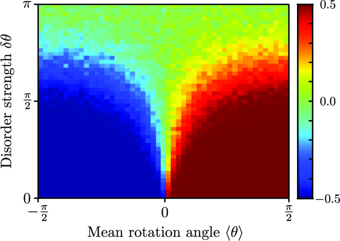
Figure 4: Disorder averaged invariant $\langle Q_{{\rm ch},0}\rangle$ at $\varepsilon=0$ for the simple quantum walk as a function of mean rotation angle and disorder strength. The transition region around $\langle\theta\rangle=0$ is broadened with increasing disorder until the topological phases are not properly defined anymore (green region). System size is $L=50$, the average is taken over $n=100$ different disorder realizations.

VIII Experiment

The scattering matrix of a discrete-time quantum walk is not only a theoretical construct but can also be directly measured. In this section we discuss the principle of such an experiment using the example of the split-step walk, introduced in Section VII.1. For the split-step walk, the reflection matrices are real numbers of unit magnitude, $(r(0),r(\pi))=(\pm 1,\pm 1)$, and, using (19), the pair of topological invariants simplify to

$$\mathcal{Q}_{\rm ch,0} =\frac{1}{2}\sum_{\nu=1}^{\infty}\langle{-1,\downarrow}|\mathcal{F}^{\nu}|{-1,\uparrow}\rangle;$$

$$\mathcal{Q}_{\rm ch,\pi} =\frac{1}{2}\sum_{\nu=1}^{\infty}(-1)^{\nu}\langle{-1,\downarrow}|\mathcal{F}^{\nu}|{-1,\uparrow}\rangle.$$ (42)

These formulas suggest a measurement protocol for the topological invariants: 1) Initialize the walk with the walker at time $\tau=0$ at $x=-1$, in state $\uparrow$. 2) Obtain the topological invariants as the sum, and alternating sum of the probability amplitudes for the walker at timestep $\tau\in\mathbb{N}$ to be at $x=-1$, in state $\downarrow$. This measurement can be straightforwardly conceived in optical realizations of quantum walks, as we show below.

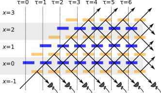
Figure 5: Schematic layout for the experimental measurement of the reflection amplitudes of a split-step quantum walk. An incident coherent light pulse at $\tau=0$, $x=-1$ enters an array of beam splitters of two types (dark blue, light orange), where it is split and recombined repeatedly, thereby performing the quantum walk. A row of detectors at $x=-1$ measure the wave amplitudes $\langle{-1,\downarrow}|\mathcal{F}^{\tau}|{-1,\uparrow}\rangle$ leaving the quantum walk region. The reflection amplitudes $r(0)$ and $r(\pi)$ are given by the sum and and the alternating sum of the measured reflected amplitudes, Eqs. (42).

We demonstrate our ideas using a simple beam splitter (BS) representation of the quantum walk, shown in Fig. 5. This layout can be easily adapted to many actual physical realizations, including integrated photonics,Sansoni et al. (2012) or even optical feedback loops. Schreiber et al. (2012) It consists of an array of cascaded BS’s, with a light pulse incident on the lower left BS. As the light propagates in time, it spreads throughout the array in a way that can be interpreted as a quantum walk. The state of the light just before and just after the $n$th column of BS’s is mapped to the state of the walker just before and just after the $n$th rotation operation. The direction of propagation of the modes is identified with the internal state of the walker, “right-up” representing $\uparrow$ and “right-down” representing $\downarrow$. The vertical coordinate in the arrays is identified with the position $x$ of the walker, as indicated in Fig. 5. We use two different types of BS’s to realize the two rotations in the Floquet operator, Eq. (36).

In optical DTQW experiments, intensity measurements on the modes leaving the array at the right edge are used to read out the position distribution of the walker after $\tau$ steps. In our case, there are two differences. First, as indicated in Fig. 5, our output modes are not at the right edge, but rather at the bottom edge of the array. Second, intensity measurement on the output modes does not work for us, since it destroys the phase information that is crucial to obtain the topological invariants, as sums of probability amplitudes, Eq. (42).

A direct measurement of the probability amplitudes as required for the invariants is possible if the incident light pulse is a strong coherent state $|{\alpha}\rangle$, containing many photons. This is standard practice in some photonic quantum walk experiments.Schreiber et al. (2012) Strictly speaking the spreading of the light pulse is then not a quantum walk any more, since there is no entanglement at any point in the system. However, it simulates a single-photon quantum walk directly. At any time, the array contains coherent states $\Pi_{j}|{\alpha_{j}}\rangle$, with the coherent amplitudes $\alpha_{j}$ corresponding exactly to the probability amplitudes $\Psi_{j}$ of the walker, $\Psi_{j}=\alpha_{j}/\alpha$. This is used in experimentsSchreiber et al. (2010) to read out the state of the walker during the walk, and to measure the probability distribution after $N$ steps in one shot.

The $0$ and $\pi$ quasienergy invariants are obtained by measuring the sum and the alternating sum of the outcoming coherent amplitudes, cf. Eqs. (42). This can be done practically by interfering each output mode with a local oscillator, or, interfering the output modes directly with each other on an N-port. Note that since the BS’s have only real elements (no phase shifting), a single intensity measurement suffices. Moreover, in this setup, one can even use a CW laser instead of a laser pulse.

IX Conclusion

In this paper we have classified the topological phases of one-dimensional discrete-time quantum walks using a scattering matrix approach. For this purpose, we generalised the concept of the scattering matrix to these periodically time-dependent systems.

We find that, dependent on their symmetries, gapped DTQWs are characterised by one of three different topological invariants, $\mathcal{Q}_{\rm D}$, $\mathcal{Q}_{\rm DIII}$ and $\mathcal{Q}_{\rm ch}$. They are calculated from the determinant, Pfaffian or trace of the reflection matrix as summarised in Table 1. In contrast to their analogs for time-independent systems,Fulga et al. (2011) the invariants consist of two independent contributions $\mathcal{Q}=\mathcal{Q}_{0}\times\mathcal{Q}_{\pi}$ that are evaluated at the two special quasienergies $\varepsilon=0,\pi$. Adapting arguments for topological insulators,Fulga et al. (2011) we found that an interface between two extended quantum walk regions hosts a number of protected boundary states that equals the difference of the invariants across the interface. These are stationary states of the walk where the walker stays exponentially close to the interface, and has quasienergy $\varepsilon=0$ or $\varepsilon=\pi$.

We also considered unbalanced DTQWs where there is a difference $n$ in the number of left- and rightward shifts per cycle, producing a quasienergy winding in the Brillouin zone. We found that they have $n$ channels that transmit perfectly in the majority direction. The characterization of transmission in this problem, including the transport time distribution of disordered quantum walks with quasienergy winding, poses an interesting direction for further investigation.

We provide a simple scheme to directly measure the reflection matrix – and, thus, the topological invariants – of a quantum walk. This scheme is well within the reach of current experiments working with light pulses Peruzzo et al. (2010); Sansoni et al. (2012); Schreiber et al. (2012, 2010).

Our scattering matrix approach complements existing methods based on Floquet operators in momentum space, with two important advantages. First, we provide a unified framework describing topological phases in different symmetry classes as simple functions of a single, typically small matrix. Second, our formulas use only a single time frame for the Floquet operator. This is in contrast with Ref. Asbóth and Obuse, 2013, which explicitly states that the topological invariants of chiral quantum walks can only be obtained by combining the winding numbers from different timeframes. The scattering matrix gets around this restriction, and probes the behaviour of the system during a protocol by including contributions from plane wave-like modes that enter and exit the scattering region at intermediate times.

The scattering matrix formalism introduced in this paper gives a powerful new tool for the investigation of the effects of disorder on topological phases and transport in DTQWs. Depending on the types of disorder and symmetries, experiments and theory on DTQWs have already seen both Anderson localization, Schreiber et al. (2011) and delocalization. Obuse and Kawakami (2011) Our generalized scattering matrix formalism allows a continuation of this research to more general multistep DTQWs.

Appendix A Numerical implementation

According to Eq. (19) the scattering matrix is determined by following the time evolution of a particle which is placed in an incoming mode until it enters an outgoing mode. While doing so, most of the infinite Hilbert space of the scattering problem will not be reached by the particle. Consequently, we can evaluate this formula in a modified, finite Hilbert space.

We thus introduce a reduced circular system, which contains all states of the $L$ sites in the system, and additional “buffer” states, which we now describe. Consider all lead states that are localised on a single lead site only and, after one period, will be shifted into the scattering region. These are the only lead states which are non-trivially involved during one time step, all other lead states are just shifted according to the lead propagator. Likewise, consider all localised lead states that are reached from the scattering region during one period. These two groups of states are arranged symmetrically with respect to the scattering center: Whenever a shift operator moves a state into the scattering region from one side, a corresponding state on the other side of the system is moved out of the system. To form the reduced finite space, we identify such pairs of lead states with each other. Each pair forms one of the buffer states, which in turn form a circular system when combined with the scattering region.

In summary, there are $d_{n}$ buffer states and $L$ system states in the reduced space for each internal state $n$. For exactly one time period, the time evolution of this finite system will be the same as for the original infinite system.

We can use this system to describe the complete scattering process, if before each step we initialize the buffer states with a wave function from the incoming leads, propagate for one unit of time, and then unload the buffer states as the outgoing mode. Denoting by $\psi_{\text{sys}}$ the wave function on the scattering sites and by $\psi_{\text{in/out}}$ the states of the buffer, the dynamics are described by:

$$\begin{pmatrix}\psi_{\rm sys}\left(t+1\right)\\ \psi_{\rm out}\left(t+1\right)\end{pmatrix}=V\begin{pmatrix}\psi_{\rm sys}\left(t\right)\\ \psi_{\rm in}\left(t\right)\end{pmatrix}=\begin{pmatrix}A&w_{\text{in}}\\ w_{\text{out}}&S_{0}\end{pmatrix}\begin{pmatrix}\psi_{\rm sys}\left(t\right)\\ \psi_{\rm in}\left(t\right)\end{pmatrix},$$ (43)

where the matrix $V$ describes the effect of $\mathcal{F}$ on this reduced space. We note that this form corresponds to the standard form for discrete-time scattering problems given in Ref. Fyodorov and Sommers, 2000.

We can write $V$ in terms of modified shift and rotation operators:

$$V=V_{S}^{(M)}V_{R}^{(M)}\cdots V_{S}^{(2)}V_{R}^{(2)}V_{S}^{(1)}V_{R}^{(1)}.$$ (44)

Here, the effect of $S^{\left(j\right)}$ on our reduced space is given by a shift matrix

$$V_{S}^{\left(j\right)} =\sum_{n}\sum_{x=-d_{n}}^{L}|{x+s_{n_{j}},n}\rangle\langle{x,n}|,$$ (45)

which is circular because of the identification of incoming and outgoing localized states $|{L+1,n}\rangle\simeq|{-d_{n},n}\rangle$. Similarly, the effect of a rotation on this space is given by

$$V_{R}=\sum_{n,n^{\prime}}\sum_{x=1}^{L}|{x,n}\rangle R_{nn^{\prime}}(x)\langle{x,n^{\prime}}|$$ (46)

$${}+\sum_{n}\sum_{x=-d_{n}}^{0}|{x,n}\rangle\langle{x,n}|,$$

applying the rotation to the system, but not to the buffer.

It can then be shownFyodorov and Sommers (2000) that the scattering matrix (reflection and transmission) can be obtained from the finite matrix $V$ by

$$S =w_{\text{out}}\left(e^{-i\varepsilon}-A\right)^{-1}w_{\text{in}}+S_{0},$$ (47)

in contrast to Eq. (19) which is defined on an infinite space.

Appendix B Symmetries of the reflection matrix

B.1 Derivation of the symmetry relations

We demonstrate how we obtain the symmetry relations Eqs. (26), (27), (25) for the reflection matrix. Assume that we are given a scattering state with one incoming mode ($n\in M_{+}$), so that

$$\left(\varepsilon-H_{\text{eff}}\right)\left[|{l_{n,d,\varepsilon}}\rangle+r|{l_{n,d,\varepsilon}}\rangle+|{\Psi_{C}}\rangle\right] =0.$$ (48)

The first term is the incoming mode and the second term describes the corresponding reflected modes, where we use operator notation for the reflection matrix:

$$r|{l_{n,d,\varepsilon}}\rangle =\sum_{n^{\prime}\in M_{-}}\sum_{d^{\prime}=1}^{d_{n^{\prime}}}r_{n^{\prime}d^{\prime},nd}|{l_{n^{\prime},d^{\prime},\varepsilon}}\rangle.$$ (49)

The third term describes the wavefunction within the scatterer, cf. Eq. (16).

By application of the TRS operator $\mathcal{T}$ on Eq. (48), using the fact that it commutes with $H_{\text{eff}}$, and employing the representation of TRS on the scattering states, Eq. (24), we find that

$$\left(\varepsilon-H_{\text{eff}}\right)\left[Q_{T}|{l_{n,d,\varepsilon}}\rangle+V_{T}r^{*}|{l_{n,d,\varepsilon}}\rangle+\mathcal{T}|{\Psi_{C}}\rangle\right] =0,$$ (50)

where the complex conjugation occurs due to the antiunitarity of $\mathcal{T}$.

Thus we constructed another scattering state at energy $\varepsilon$, where the incoming modes are the time-reversed former outgoing modes: $V_{T}r\left(\varepsilon\right)^{*}|{l_{n,d,\varepsilon}}\rangle$, and outgoing modes are constructed from the time-reversed incoming mode: $Q_{T}|{l_{n,d,\varepsilon}}\rangle$. By the definition of $r$, we thus must have the relation

$$r\left(\varepsilon\right)V_{T}r\left(\varepsilon\right)^{*}|{l_{n,d,\varepsilon}}\rangle =Q_{T}|{l_{n,d,\varepsilon}}\rangle,$$ (51)

and as this holds for all $n\in M_{+}$ and corresponding $d$, we can conclude Eq. (26). Analogous arguments can be given to show Eq. (27) and Eq. (28).

B.2 Basis transformations

We next consider basis transformations of the incoming and outgoing modes in order to turn the symmetries of $r$ presented in Eqs. (26) to (28) into standard form. Because the incoming and outgoing modes are separate spaces, we can choose basis transformations for both independently. This amounts to a multiplication of $r$ with two unrelated unitary matrices from the left and right respectively.

In the following we assume that $r$ is taken at energies $\varepsilon=0,\pi$ and we suppress energy dependence.

Class D

If $\mathcal{P}^{2}=1$, it can be seen that $Q_{P\pm}=Q_{P\pm}^{T}$. Thus, we can find square roots $M^{2}_{\pm}=Q_{P,\pm}$, which are also symmetric. It can then be checked that after the transformation

$$\tilde{r} =M_{-}^{*}rM_{+}^{T},$$ (52)

Eq. (28) is equivalent to $\tilde{r}=\tilde{r}^{*}$.

Class DIII

If $\mathcal{T}^{2}=-1$, one can see that $Q_{T}^{T}=-V_{T}$. Again, we can find symmetric square roots,

$$M_{+}^{2} =Q_{P,+},$$ (53)

$$M_{-}^{2} =Q_{T}^{\dagger}Q_{P,-}Q_{T}^{*},$$ (54)

and performing the basis transformation

$$\tilde{r} =M_{-}^{*}V_{T}^{*}rM_{+}^{T},$$ (55)

this leads from Eqs. (26) and (28) to $\tilde{r}=\tilde{r}^{*}=-\tilde{r}^{T}$. Importantly, one uses the fact that because of assumed irreducibility of any unitary symmetry operator, by Schur’s lemma we must have $\mathcal{PTPT}=e^{i\phi}$, from which one finds that $M_{-}M_{+}^{T}=e^{-i\phi/2}$.

Chiral classes

For these classes, we have a chiral operator, obeying $V_{\Gamma}Q_{\Gamma}=\Gamma^{2}=1$. Then we can choose $\tilde{r}=V_{\Gamma}r$ and from Eq. (27) find $\tilde{r}=\tilde{r}^{\dagger}$.

We note that these transformation are not unique (for instance, in class D, any orthogonal transformation preserves $\tilde{r}=\tilde{r}^{*}$) , so that other possible choices exist. The actual value of topological invariants obtained from $\tilde{r}$ depend on the choice. However, because there is no unambigious notion of a trivial vacuum for quantum walk systems, we do not impose further restrictions on the choice of basis, and instead remark that the definition of topological invariants is only possible after fixing a specific suitible basis.

Appendix C Protected boundary states

Here we derive the existence of protected boundary states caused by a change of topology across an interface between two domains with a different DTQW protocol. We exemplify the derivation for a class D quantum walk. For other symmetry classes, one can argue in a similar fashion. Fulga et al. (2011)

If two compatible DTQWs, a left (A) and right (B) one, are interfaced, a bound state occurs at the interface whenever $\det(1-r_{A}r^{\prime}_{B})=0$, where $r^{\prime}$ denotes the reflection matrix for incoming states from the right. Consider a fixed energy $\varepsilon\in 0,\pi$. The reflection matrices $r_{A}$ and $r^{\prime}_{B}$ are orthogonal matrices at this energy, as is their product. Thus, $\det{(r_{A}r^{\prime}_{B})}=\pm 1$.

The determinant $\det{(r_{A}r^{\prime}_{B})}$ is the product of the eigenvalues of an orthogonal matrix, which in term come either in complex conjugate pairs or are $1$ or $-1$.

For even matrix size and $\det{(r_{A}r^{\prime}_{B})}=-1$, an odd number of eigenvalues has to be $-1$ and thus at least one eigenvalue $1$. An eigenvalue of $1$ amounts to a bound state at the given energy. For odd matrix size on the other hand, a positive determinant requires at least one eigenvalue $1$ and thereby ensures a bound state.

To connect these bound states to the topological invariant $\mathcal{Q}_{\text{D}}$, we first need to understand the relation between $r$ and $r^{\prime}$. This can be deduced by requiring that by connecting two copies of the same quantum walk, no bound states should exist (they would be states in the middle of a gap). Thus for even matrix dimension, $\det r=\det r^{\prime}$ while for odd matrix dimension $\det r=-\det r^{\prime}$.

In conclusion this means that, when $\det r_{A}\neq\det r_{B}$, a bound state between the two regions is ensured by the change of topology across the boundary.

References

- Hasan and Kane (2010) M. Z. Hasan and C. L. Kane, Rev. Mod. Phys. 82, 3045 (2010), URL http://link.aps.org/doi/10.1103/RevModPhys.82.3045.
- Qi and Zhang (2011) X.-L. Qi and S.-C. Zhang, Rev. Mod. Phys. 83, 1057 (2011), URL http://link.aps.org/doi/10.1103/RevModPhys.83.1057.
- Ando (2013) Y. Ando, Journal of the Physical Society of Japan 82, 102001 (2013), URL http://jpsj.ipap.jp/link?JPSJ/82/102001/.
- Aidelsburger et al. (2013) M. Aidelsburger, M. Atala, M. Lohse, J. T. Barreiro, B. Paredes, and I. Bloch, Phys. Rev. Lett. 111, 185301 (2013), URL http://link.aps.org/doi/10.1103/PhysRevLett.111.185301.
- Kraus and Zilberberg (2012) Y. E. Kraus and O. Zilberberg, Phys. Rev. Lett. 109, 116404 (2012), URL http://link.aps.org/doi/10.1103/PhysRevLett.109.116404.
- Sun et al. (2012) K. Sun, W. V. Liu, A. Hemmerich, and S. Das Sarma, Nature Physics 8, 67 (2012), URL http://dx.doi.org/10.1038/nphys2134.
- Venegas-Andraca (2012) S. Venegas-Andraca, Quantum Information Processing 11, 1015 (2012), ISSN 1570-0755, URL http://dx.doi.org/10.1007/s11128-012-0432-5.
- Bhattacharya et al. (2002) N. Bhattacharya, H. B. van Linden van den Heuvell, and R. J. C. Spreeuw, Phys. Rev. Lett. 88, 137901 (2002), URL http://link.aps.org/doi/10.1103/PhysRevLett.88.137901.
- Lovett et al. (2010) N. B. Lovett, S. Cooper, M. Everitt, M. Trevers, and V. Kendon, Phys. Rev. A 81, 042330 (2010), URL http://link.aps.org/doi/10.1103/PhysRevA.81.042330.
- Karski et al. (2009) M. Karski, L. Förster, J.-M. Choi, A. Steffen, W. Alt, D. Meschede, and A. Widera, Science 325, 174 (2009), URL http://www.sciencemag.org/content/325/5937/174.abstract.
- Genske et al. (2013) M. Genske, W. Alt, A. Steffen, A. H. Werner, R. F. Werner, D. Meschede, and A. Alberti, Phys. Rev. Lett. 110, 190601 (2013), URL http://link.aps.org/doi/10.1103/PhysRevLett.110.190601.
- Schmitz et al. (2009) H. Schmitz, R. Matjeschk, C. Schneider, J. Glueckert, M. Enderlein, T. Huber, and T. Schaetz, Phys. Rev. Lett. 103, 090504 (2009), URL http://link.aps.org/doi/10.1103/PhysRevLett.103.090504.
- Zähringer et al. (2010) F. Zähringer, G. Kirchmair, R. Gerritsma, E. Solano, R. Blatt, and C. F. Roos, Phys. Rev. Lett. 104, 100503 (2010), URL http://link.aps.org/doi/10.1103/PhysRevLett.104.100503.
- Peruzzo et al. (2010) A. Peruzzo, M. Lobino, J. C. F. Matthews, N. Matsuda, A. Politi, K. Poulios, X.-Q. Zhou, Y. Lahini, N. Ismail, K. Wörhoff, et al., Science 329, 1500 (2010), URL http://www.sciencemag.org/content/329/5998/1500.abstract.
- Broome et al. (2010) M. A. Broome, A. Fedrizzi, B. P. Lanyon, I. Kassal, A. Aspuru-Guzik, and A. G. White, Phys. Rev. Lett. 104, 153602 (2010), URL http://link.aps.org/doi/10.1103/PhysRevLett.104.153602.
- Schreiber et al. (2012) A. Schreiber, A. Gábris, P. P. Rohde, K. Laiho, M. Štefaňák, V. Potoček, C. Hamilton, I. Jex, and C. Silberhorn, Science 336, 55 (2012), URL http://www.sciencemag.org/content/336/6077/55.abstract.
- Schreiber et al. (2010) A. Schreiber, K. N. Cassemiro, V. Potoček, A. Gábris, P. J. Mosley, E. Andersson, I. Jex, and C. Silberhorn, Phys. Rev. Lett. 104, 050502 (2010), URL http://link.aps.org/doi/10.1103/PhysRevLett.104.050502.
- Sansoni et al. (2012) L. Sansoni, F. Sciarrino, G. Vallone, P. Mataloni, A. Crespi, R. Ramponi, and R. Osellame, Phys. Rev. Lett. 108, 010502 (2012), URL http://link.aps.org/doi/10.1103/PhysRevLett.108.010502.
- Jeong et al. (2013) Y.-C. Jeong, C. D. Franco, H.-T. Lim, M. Kim, and Y.-H. Kim, Nature Communications 4, 2471 (2013).
- Kitagawa et al. (2010a) T. Kitagawa, M. S. Rudner, E. Berg, and E. Demler, Phys. Rev. A 82, 033429 (2010a), URL http://link.aps.org/doi/10.1103/PhysRevA.82.033429.
- Kitagawa et al. (2012) T. Kitagawa, M. A. Broome, A. Fedrizzi, M. S. Rudner, E. Berg, I. Kassal, A. Aspuru-Guzik, E. Demler, and A. G. White, Nature Communications 3, 882 (2012).
- Ryu et al. (2010) S. Ryu, A. P. Schnyder, A. Furusaki, and A. W. W. Ludwig, New Journal of Physics 12, 065010 (2010).
- Lindner et al. (2011) N. H. Lindner, G. Refael, and V. Galitski, Nature Physics 7, 490–495 (2011).
- Cayssol et al. (2013) J. Cayssol, B. Dóra, F. Simon, and R. Moessner, Phys. Status Solidi RRL 7, 101 (2013).
- Kitagawa et al. (2010b) T. Kitagawa, E. Berg, M. Rudner, and E. Demler, Phys. Rev. B 82, 235114 (2010b), URL http://link.aps.org/doi/10.1103/PhysRevB.82.235114.
- Jiang et al. (2011) L. Jiang, T. Kitagawa, J. Alicea, A. R. Akhmerov, D. Pekker, G. Refael, J. I. Cirac, E. Demler, M. D. Lukin, and P. Zoller, Phys. Rev. Lett. 106, 220402 (2011), URL http://link.aps.org/doi/10.1103/PhysRevLett.106.220402.
- Rudner et al. (2013) M. S. Rudner, N. H. Lindner, E. Berg, and M. Levin, Phys. Rev. X 3, 031005 (2013), URL http://link.aps.org/doi/10.1103/PhysRevX.3.031005.
- Kitagawa (2012) T. Kitagawa, Quantum Information Processing 11, 1107 (2012).
- Akhmerov et al. (2011) A. R. Akhmerov, J. P. Dahlhaus, F. Hassler, M. Wimmer, and C. W. J. Beenakker, Phys. Rev. Lett. 106, 057001 (2011), URL http://link.aps.org/doi/10.1103/PhysRevLett.106.057001.
- Fulga et al. (2011) I. C. Fulga, F. Hassler, A. R. Akhmerov, and C. W. J. Beenakker, Phys. Rev. B 83, 155429 (2011), URL http://link.aps.org/doi/10.1103/PhysRevB.83.155429.
- Dahlhaus et al. (2012) J. P. Dahlhaus, M. Gibertini, and C. W. J. Beenakker, Phys. Rev. B 86, 174520 (2012), URL http://link.aps.org/doi/10.1103/PhysRevB.86.174520.
- Asbóth and Obuse (2013) J. K. Asbóth and H. Obuse, Phys. Rev. B 88, 121406 (2013), URL http://link.aps.org/doi/10.1103/PhysRevB.88.121406.
- Meyer (1997) D. A. Meyer, Phys. Rev. E 55, 5261 (1997), URL http://link.aps.org/doi/10.1103/PhysRevE.55.5261.
- Feldman and Hillery (2005) E. Feldman and M. Hillery, Contemporary Mathematics 381, 71 (2005).
- Feldman and Hillery (2007) E. Feldman and M. Hillery, Journal of Physics A: Mathematical and Theoretical 40, 11343 (2007), URL http://stacks.iop.org/1751-8121/40/i=37/a=011.
- Altland and Zirnbauer (1997) A. Altland and M. R. Zirnbauer, Phys. Rev. B 55, 1142 (1997), URL http://link.aps.org/doi/10.1103/PhysRevB.55.1142.
- Fulga et al. (2012) I. C. Fulga, F. Hassler, and A. R. Akhmerov, Phys. Rev. B 85, 165409 (2012), URL http://link.aps.org/doi/10.1103/PhysRevB.85.165409.
- Asbóth (2012) J. K. Asbóth, Phys. Rev. B 86, 195414 (2012), URL http://link.aps.org/doi/10.1103/PhysRevB.86.195414.
- Schreiber et al. (2011) A. Schreiber, K. N. Cassemiro, V. Potoček, A. Gábris, I. Jex, and C. Silberhorn, Phys. Rev. Lett. 106, 180403 (2011), URL http://link.aps.org/doi/10.1103/PhysRevLett.106.180403.
- Obuse and Kawakami (2011) H. Obuse and N. Kawakami, Phys. Rev. B 84, 195139 (2011), URL http://link.aps.org/doi/10.1103/PhysRevB.84.195139.
- Fyodorov and Sommers (2000) Y. Fyodorov and H.-J. Sommers, Journal of Experimental and Theoretical Physics Letters 72, 422 (2000), ISSN 0021-3640, URL http://dx.doi.org/10.1134/1.1335121.