Adjoint method for a tumor invasion PDE-constrained optimization problem using FEM

Abstract

In this paper we present a method for estimating unknown parameter that appear on a non-linear reaction-diffusion model of cancer invasion. This model considers that tumor-induced alteration of micro-enviromental pH provides a mechanism for cancer invasion. A coupled system reaction-diffusion describing this model is given by three partial differential equations for the non dimensional spatial distribution and temporal evolution of the density of normal tissue, the neoplastic tissue growth and the excess concentration of H⁺ ions. Each of the model parameters has a corresponding biological interpretation, for instance, the growth rate of neoplastic tissue, the diffusion coefficient, the reabsorption rate and the destructive influence of H⁺ ions in the healthy tissue.

After solving the forward problem properly, we use the model for the estimation of parameters by fitting the numerical solution with real data, obtained via in vitro experiments and fluorescence ratio imaging microscopy. We define an appropriate functional to compare both the real data and the numerical solution using the adjoint method for the minimization of this functional.

We apply Finite Element Method (FEM) to solve both the direct and inverse problem, computing the a posteriori error.

1 Introduction.

Cancer is one of the greatest killers in the world although medical activity has been successful, despite great difficulties, at least for some pathologies. A great effort of human and economical resources is devoted, with successful outputs, to cancer research, [1, 2, 3, 4, 5, 6].

Some comments on the importance of mathematical modeling in cancer can be found in the literature. In the work [4] the authors say “Cancer modelling has, over the years, grown immensely as one of the challenging topics involving applied mathematicians working with researchers active in the biological sciences. The motivation is not only scientific as in the industrial nations cancer has now moved from seventh to second place in the league table of fatal diseases, being surpassed only by cardiovascular diseases.”

We use in this work the mathematical analyses first proposed by [7] which supports the acid-mediated invasion hypothesis, hence it is acquiescent to mathematical representation as a reaction-diffusion system at the tissue scale, describing the spatial distribution and temporal development of tumor tissue, normal tissue, and excess H⁺ ion concentration.

The model predicts a pH gradient extending from the tumor-host interface. The effect of biological parameters critical to controlling this transition is supported by experimental and clinical observations [8].

In [7] the authors model tumor invasion in an attempt to find a common, underlying mechanism by which primary and metastatic cancers invade and destroy normal tissues. They are not modeling the genetic changes which result in transformation nor do they seek to understand the causes of these changes. Similarly, they do not attempt to model the large-scale morphological features of tumors such as central necrosis. Rather, they concentrate on the microscopic scale population interactions occurring at the tumor-host interface, reasoning that these processes strongly influence the clinically significant manifestations of invasive cancer.

Specifically, the authors hypothesize that transformation-induced reversion of neoplastic tissue to primitive glycolytic metabolic pathways, with resultant increased acid production and the diffusion of that acid into surrounding healthy tissue, creates a peritumoral microenvironment in which tumor cells survive and proliferate, whereas normal cells are unable to remain viable. The following temporal sequence would derive: (a) high H⁺ ion concentrations in tumors will extend, by chemical diffusion, as a gradient into adjacent normal tissue, exposing these normal cells to tumor-like interstitial pH; (b) normal cells immediately adjacent to the tumor edge are unable to survive in this chronically acidic environment; and (c) the progressive loss of layers of normal cells at the tumor-host interface facilitates tumor invasion. Key elements of this tumor invasion mechanism are low interstitial pH of tumors due to primitive metabolism and reduced viability of normal tissue in a pH environment favorable to tumor tissue.

These model equations depend only on a small number of cellular and subcellular parameters. Analysis of the equations shows that the model predicts a crossover from a benign tumor to one that is aggressively invasive as a dimensionless combination of the parameters increases through a critical value.

The dynamics and structure of the tumor-host interface in invasive cancers are shown to be controlled by the same biological parameters which generate the transformation from benign to malignant growth. A hypocellular interstitial gap, as we can see in Figure 1 [7, Figure 4a], at the interface is predicted to occur in some cancers.

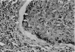
Figure 1: A micrographs of the tumor-host interface from human squamous cell carcinomas of the head and neck [7].

In this paper we estimate one of these parameters (the destructive influence of H⁺ ions in the healthy tissue) using an inverse problem. Moreover, via fluorescence ratio imaging microscopy, it is possible get data about the concentration of hydrogen ions [8]. We propose a framework via a PDE-constrained optimization problem, following the PDE-based model by Gatenby [7]. In this approach, tumor invasion is modeled via a coupled nonlinear system of partial differential equations, which makes the numerical solution procedure quite challenging.

This kind of problem constitutes a particular application of the so-called inverse problems, which are being increasingly used in a broad number of fields in applied sciences. For instance, problems referred to structured population dynamics [9], computerized tomography and image reconstruction in medical imaging [10, 11], and more specifically tumor growth [12, 13, 14], among many others.

We solve a minimization problem using a gradient-based method considering the adjoint method in order to find the derivative of an objective functional. In this way, we would obtain the best parameter that fits patient-specific data.

The contents of this paper, which is organized into 9 sections and an Appendix, are as follows: Section 2 consists in some preliminaries about the model and the definition of the direct problem. Section 3 deals with the variational formulation of the direct problem. Section 4 considers the formulation of the minimization problem. Section 5 introduces the reduced and adjoint problem, deriving the optimality conditions for the problem. Section 6 finds the derivative of the solution of a functional with respect to a parameter that does not appear explicitly in the equation. Section 7 deals with the numerical solution of the adjoint problem, designing a suitable algorithm to solve it. In particular, we use the Finite Element Method with a computation of a posteriori error. In Section 8 we show some numerical simulations to give information on the behavior of the functional and its dependence on the parameters including the corresponding tables. Section 9 presents the conclusions and some future work related to the contents of this paper. In the Appendix we include all algebraics of Section 6.

Some words about our notation. We use $\langle\cdot,\cdot\rangle$ to denote the $L^{2}$ inner product (the space is always clear from the context) and we consider the sum of inner products for a cartesian product of spaces. For a function $F:V\times U_{ad}\rightarrow\mathcal{Z}$ such that $(u,\delta_{1})\mapsto F(u,\delta_{1})$, we denote by $F^{\prime}(u,\delta_{1})$ the full Fréchet-derivative and by $\frac{\partial F}{\partial u}(u,\delta_{1})$ and $\frac{\partial F}{\partial\delta_{1}}(u,\delta_{1})$ the partial Fréchet-derivatives of $F$ at $(u,\delta_{1})$. For a linear operator $T:V\rightarrow\mathcal{Z}$ we denote $T^{*}:\mathcal{Z}^{*}\rightarrow V^{*}$ the adjoint operator of $T$. If $T$ is invertible, we call $T^{-*}$ the inverse of the adjoint operator $T^{*}$.

2 Some preliminaries about the model.

We present the mathematical model of the tumor-host interface based on the acid mediation hypothesis of tumor invasion due to [7]. For convenience we reproduce the equations here, which determine the spatial distribution and temporal evolution of three fields: $N_{1}(x,t)$, the density of normal tissue; $N_{2}(x,t)$, the density of neoplastic tissue; and $L(x,t),$ the excess concentration of H⁺ ions. The units of $N_{1}$ and $N_{2}$ are cells/cm³ and excess H⁺ ion concentration is expressed as a molarity (M), $x$ and $t$ are the position (in cm) and time (in seconds), respectively.

$$\frac{\partial N_{1}}{\partial t} = r_{1}N_{1}\left(1-\frac{N_{1}}{K_{1}}\right)-d_{1}LN_{1},$$ (1)

$$\frac{\partial N_{2}}{\partial t} = r_{2}N_{2}\left(1-\frac{N_{2}}{K_{2}}\right)+\nabla\cdot\left(D_{N_{2}}\left(1-\frac{N_{1}}{K_{1}}\right)\nabla N_{2}\right),$$ (2)

$$\frac{\partial L}{\partial t} = r_{3}N_{2}-d_{3}L+D_{N_{3}}\Delta L,$$ (3)

where the variables are in $\Omega\times[0,T]$.

In equation (1) the behavior of the normal tissue is determined by the logistic growth of $N_{1}$ with growth rate $r_{1}$ and carrying capacity $K_{1}$, and the interaction of $N_{1}$ with excess H⁺ ions leading to a death rate proportional to $L$. The number $d_{1}L$ is the excess acid concentration, dependent death rate in accord with the well-described decline in the growth rate of normal cells, due to the reduction of pH from its optimal value of $7.4$. The constants $r_{1}$, $d_{1}$ and $K_{1}$ have units of $1/$s, l/(M s) and cells/cm³, respectively.

For equation (2), the neoplastic tissue growth is described by a reaction-diffusion equation. The reaction term is governed by a logistic growth of $N_{2}$ with growth rate $r_{2}$ and carrying capacity $K_{2}$. The diffusion term depends on the absence of healthy tissue with a diffusion constant $D_{N_{2}}$. Constants $r_{2}$, $K_{2}$ and $D_{N_{2}}$ have units of $1/$s, cells/cm³ and cm²/s, respectively.

In equation (3), it is assumed that excess H⁺ ions are produced at a rate proportional to the neoplastic cell density, and diffuse chemically. An uptake term is included to take account of the mechanisms for increasing local pH (e.g., buffering and large-scale vascular evacuation [7]). Constant $r_{3}$ is the production rate (M cm³/(cell s)), $d_{3}$ is the reabsorption rate (1/s), and $D_{N_{3}}$ is the H⁺ ion diffusion constant (cm²/s).

All the parameter values can be found in Table 1.

Parameter	Estimate
$K_{1}$	$5\times 10^{7}/$cm3
$K_{2}$	$5\times 10^{7}/$cm3
$r_{1}$	$1\times 10^{-6}/$s
$r_{2}$	$1\times 10^{-6}/$s
$D_{N_{2}}$	$2\times 10^{-10}$cm${}^{2}/$s
$D_{N_{3}}$	$5\times 10^{-6}$cm${}^{2}/$s
$r_{3}$	$2.2\times 10^{-17}$M cm${}^{3}/$s
$d_{3}$	$1.1\times 10^{-4}/$s

Table 1: Parameter values used in [7].

2.1 Nondimensionalization.

Following the ideas exposed in [7], and considering that $\Omega\subset\mathbbm{R}$, the mathematical model is rescaled and the domain is transformed onto the interval $[0,1]\times[0,T]$. Hence, let us define the following functions:

$$\begin{array}[]{lcl c lcl}\displaystyle u_{1}&=&\displaystyle\frac{N_{1}}{K_{1}}&&\displaystyle u_{2}&=&\displaystyle\frac{N_{2}}{K_{2}}\\[8.53581pt] \displaystyle u_{3}&=&\displaystyle\frac{L}{L_{0}}&&\displaystyle\tau&=&\displaystyle r_{1}t\\[8.53581pt] \displaystyle\xi&=&\displaystyle\sqrt{\frac{r_{1}}{D_{N_{3}}}}x&&&&\end{array}$$ (4)

where $L_{0}=r_{3}K_{2}/d_{3}$. We will continue denoting $x$ and $t$ instead of $\xi$ and $\tau$, respectively. Using the transformation (4) the dimensionless form of the equations (1)-(3) become

$$\frac{\partial u_{1}}{\partial t} = u_{1}(1-u_{1})-\delta_{1}u_{1}u_{3},$$ (5)

$$\frac{\partial u_{2}}{\partial t} = \rho_{2}u_{2}(1-u_{2})+\frac{\partial}{\partial x}\left(D_{2}(1-u_{1})\frac{\partial u_{2}}{\partial x}\right),$$ (6)

$$\frac{\partial u_{3}}{\partial t} = \delta_{3}(u_{2}-u_{3})+\frac{\partial^{2}u_{3}}{\partial x^{2}},$$ (7)

for $(x,t)\in(0,1)\times(0,T]$, where the four dimensionless quantities which parameterize the model are given by:

$$\delta_{1}=\displaystyle\frac{d_{1}r_{3}K_{2}}{d_{3}r_{1}},\qquad\rho_{2}=\displaystyle\frac{r_{2}}{r_{1}},\qquad D_{2}=\displaystyle\frac{D_{N_{2}}}{D_{N_{3}}},\qquad\delta_{3}=\displaystyle\frac{d_{3}}{r_{1}}.$$

The interaction parameters between different cells (healthy and tumor) and concentration of H⁺ are difficult to measure experimentally. This is the reason for which we propose to estimate them, so we will focus on $\delta_{1}$ in this work. The other parameters can be estimated by different techniques (see Table 1).

2.2 Initial and boundary conditions.

At $t=0$ we will consider the tumor at a certain stage of its evolution. Hence the initial conditions are:

$$u_{1}(x,0) = u_{1}^{0}(x),$$ (8)

$$u_{2}(x,0) = u_{2}^{0}(x),$$ (9)

$$u_{3}(x,0) = u_{3}^{0}(x),$$ (10)

for all $x\in[0,1]$. We assume that the tumor is on the left of the domain, in the sense that the tumor cells are not moving. Then, for all $t\in[0,T]$, we have

$$\frac{\partial u_{1}}{\partial x}(0,t)=0, u_{1}(1,t)=1,$$ (11)

$$\frac{\partial u_{2}}{\partial x}(0,t)=0, u_{2}(1,t)=0,$$ (12)

$$\frac{\partial u_{3}}{\partial x}(0,t)=0, u_{3}(1,t)=0.$$ (13)

From now on, equations (5)-(13) will be referred to as the direct problem.

3 Variational form for the direct problem.

Using the variational techniques for obtaining the weak solution of the direct problem [15, 16, 17], we define the following weak formulation:

$$0 = \int_{0}^{T}\int_{0}^{1}\lambda_{1}\left[\frac{\partial u_{1}}{\partial t}-u_{1}(1-u_{1})+\delta_{1}u_{1}u_{3}\right]dxdt+$$ (14)

$$\int_{0}^{T}\int_{0}^{1}\lambda_{2}\left[\frac{\partial u_{2}}{\partial t}-\rho_{2}u_{2}(1-u_{2})-\frac{\partial}{\partial x}\left(D_{2}(1-u_{1})\frac{\partial u_{2}}{\partial x}\right)\right]dxdt+$$

$$\int_{0}^{T}\int_{0}^{1}\lambda_{3}\left[\frac{\partial u_{3}}{\partial t}-\delta_{3}(u_{2}-u_{3})-\frac{\partial^{2}u_{3}}{\partial x^{2}}\right]dxdt,$$

where $\lambda=(\lambda_{1},\lambda_{2},\lambda_{3})$,

$$\lambda_{1},\lambda_{2},\lambda_{3}\in W=\left\{v\in L^{2}(0,T;H^{1}_{D}((0,1)))\mbox{ and }\frac{\partial v}{\partial t}\in L^{2}(0,T;(H^{1}_{D}((0,1)))^{*})\right\},$$

$$L^{2}(0,T;H^{1}_{D}((0,1)))=\left\{v(x,\cdot)\in L^{2}((0,T))\mbox{ and }v(\cdot,t)\in H^{1}_{D}((0,1))\right\}$$

and

$$H^{1}_{D}=\left\{v\in H^{1}((0,1)):v=0\mbox{ on }\Gamma_{D}=\{1\}\right\}.$$

Using integration by parts and boundary condition for $\lambda$ and $u$ in (14) we get the following weak formulation of (5)-(13):

$$0 = \int_{0}^{T}\int_{0}^{1}\left(\frac{\partial u_{1}}{\partial t}\lambda_{1}-u_{1}(1-u_{1})\lambda_{1}+\delta_{1}u_{1}u_{3}\lambda_{1}\right)dxdt+$$ (15)

$$\int_{0}^{T}\int_{0}^{1}\left(\frac{\partial u_{2}}{\partial t}\lambda_{2}-\rho_{2}u_{2}(1-u_{2})\lambda_{2}+D_{2}(1-u_{1})\frac{\partial u_{2}}{\partial x}\frac{\partial\lambda_{2}}{\partial x}\right)dxdt+$$

$$\int_{0}^{T}\int_{0}^{1}\left(\frac{\partial u_{3}}{\partial t}\lambda_{3}+\delta_{3}u_{3}\lambda_{3}-\delta_{3}u_{2}\lambda_{3}+\frac{\partial u_{3}}{\partial x}\frac{\partial\lambda_{3}}{\partial x}\right)dxdt.$$

A weak solution $u=[u_{1},u_{2},u_{3}]^{T}\in V=W^{3}$ is a function that satisfies (15) for all $\lambda\in V$ and $u(x,0)=u^{0}(x)=[u^{0}_{1}(x),u^{0}_{2}(x),u^{0}_{3}(x)]$.

4 Formulation of the minimization problem.

As described above we propose to use an inverse problem technique in order to estimate $\delta_{1}$. Function $u$ represents the solution of the direct problem (the components of $u$ are the state variables of the problem) for each choice of the parameter $\delta_{1}$.

Let us assume that experimental information is available during the time interval $0\leq t\leq T$. Then, the inverse problem can be formulated as:

Find a parameter $\delta_{1}$ able to generate data $u=[u_{1},u_{2},u_{3}]^{T}$ that best match the available (experimental) information over time $0\leq t\leq T$.

For this purpose, we should construct an objective functional which gives us a notion of distance between the experimental (real) data and the solution of the system of PDEs for each choice of the parameter $\delta_{1}$.

First of all, it is important to decide which variables are capable to be measured experimentally. For instance, the excess concentration of H⁺ ions can be measured using fluorescence ratio imaging microscopy [8, 18] at certain times $t_{k}$, $k=1,\ldots,M$. For example, Figure 2 [18, Figure 4] shows a map of peritumoral H⁺ flow using vectors generated from the pH distribution around the tumor. Such experiments could help to determine optimal variables and the parameter in order to control real tumor invasion.

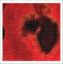
Figure 2: A map of peritumoral H⁺ flow using vectors generated from the pH distribution around the tumor, [18, Figure 4].

So, the functional $J:V\times U_{ad}\rightarrow\mathbb{R}$ could be defined as:

$$J(u,\delta_{1})=\frac{1}{2}\int_{0}^{T}\int_{0}^{1}[u_{3}(x,t)-\hat{u}_{3}(x,t)]^{2}dxdt,$$ (16)

where $u_{3}(x,t)$ is the excess concentration of H⁺ ions obtained by solving the direct problem for a certain choice of $\delta_{1}$ and $\hat{u}_{3}(x,t)$ is the excess concentration measured experimentally (real data).

Let us define $E:V\times U_{ad}\to V^{*}\times\mathcal{Z}^{*}$ such that

$$\left\langle E(u,\delta_{1}),\zeta\right\rangle = \int_{0}^{T}\int_{0}^{1}\left(\frac{\partial u_{1}}{\partial t}\lambda_{1}-u_{1}(1-u_{1})\lambda_{1}+\delta_{1}u_{1}u_{3}\lambda_{1}\right)dxdt+$$ (17)

$$\int_{0}^{T}\int_{0}^{1}\left(\frac{\partial u_{2}}{\partial t}\lambda_{2}-\rho_{2}u_{2}(1-u_{2})\lambda_{2}+D_{2}(1-u_{1})\frac{\partial u_{2}}{\partial x}\frac{\partial\lambda_{2}}{\partial x}\right)dxdt+$$

$$\int_{0}^{T}\int_{0}^{1}\left(\frac{\partial u_{3}}{\partial t}\lambda_{3}+\delta_{3}u_{3}\lambda_{3}-\delta_{3}u_{2}\lambda_{3}+\frac{\partial u_{3}}{\partial x}\frac{\partial\lambda_{3}}{\partial x}\right)dxdt+$$

$$\int_{0}^{1}(u_{1}(x,0)-u^{0}_{1}(x))\gamma_{1}dx+\int_{0}^{1}(u_{2}(x,0)-u^{0}_{2}(x))\gamma_{2}dx+$$

$$\int_{0}^{1}(u_{3}(x,0)-u^{0}_{3}(x))\gamma_{3}dx$$

$$= \left\langle\frac{\partial u}{\partial t},\lambda\right\rangle_{V^{*},V}+\left\langle F(u),\lambda\right\rangle_{V^{*},V}+\left\langle u(x,0)-u^{0}(x),\gamma\right\rangle_{\mathcal{Z}^{*},\mathcal{Z}},$$

where $\zeta=[\lambda,\gamma]$, $\gamma=[\gamma_{1},\gamma_{2},\gamma_{3}]\in\mathcal{Z}$ and $\mathcal{Z}=\left(H^{1}_{D}((0,1))\right)^{3}$.

In this way we can rewrite the weak formulation (15) as $E(u,\delta_{1})=0$.

The parameter that best matches the experimental information with the generated data provided by the direct problem can be computed by solving a PDE-constrained optimization problem, namely:

$$\begin{array}[]{rl}\displaystyle\mathop{\mathrm{minimize}}_{\delta_{1}}&J(u,\delta_{1})\\ \mathrm{subject\,to}&E(u,\delta_{1})=0,\\ &\delta_{1}\in U_{ad},\end{array}$$ (18)

where $U_{ad}$ denotes the set of admissible values of $\delta_{1}$. In our case, $U_{ad}$ should be a subset of $(0,\infty)$. Notice that a solution $(u,\delta_{1})$ must satisfy the constraint $E(u,\delta_{1})=0$, which constitutes the direct problem.

We remark that, in general, there is a fundamental difference between the direct and the inverse problems. In fact, the latter is usually ill-posed in the sense of existence, uniqueness and stability of the solution. This inconvenient is often treated by using some regularization techniques [10, 19, 20].

5 Formulation of the reduced and adjoint problems.

In the following, we will consider the so-called reduced problem

$$\begin{array}[]{rl}\displaystyle\mathop{\mathrm{minimize}}_{\delta_{1}}&\tilde{J}(\delta_{1})=J(u(\delta_{1}),\delta_{1})\\ \mathrm{subject\,to}&\delta_{1}\in U_{ad},\end{array}$$ (19)

where $u(\delta_{1})$ is given as the solution of $E(u(\delta_{1}),\delta_{1})=0$. The existence of the function $u$ is obtained by the implicit function theorem. According to the ideas exposed in [21, 22], this can be done since $U_{ad}=[0,L]$ is a nonempty, closed and convex set, $J$ and $E$ are continuously Fréchet-differentiable functions, and assuming that for each $\delta_{1}\in U_{ad}$ there exists a unique corresponding solution $u(\delta_{1})$ such that $E(u(\delta_{1}),\delta_{1})=0$ and the derivative $\frac{\partial E}{\partial u}(u(\delta_{1}),\delta_{1})$ is a continuous linear operator continuously invertible for all $\delta_{1}\in U_{ad}$.

In order to find a minimum of the continuosly differentiable function $\tilde{J}$, it will be important to compute the derivative of this reduced objective function. Hence, we will show a procedure to obtain $\tilde{J}^{\prime}$ by using the adjoint approach. Since

$$\tilde{J}^{\ \prime}(\delta_{1})=\bigl{(}u^{\prime}(\delta_{1})\bigl{)}^{*}\frac{\partial J}{\partial u}(u(\delta_{1}),\delta_{1})+\frac{\partial J}{\partial\delta_{1}}(u(\delta_{1}),\delta_{1}).$$ (20)

Let us consider $\zeta\in V\times\mathcal{Z}$ as the solution of the so-called adjoint problem:

$$\frac{\partial J}{\partial u}(u(\delta_{1}),\delta_{1})+\left(\frac{\partial E}{\partial u}(u(\delta_{1}),\delta_{1})\right)^{*}\zeta=0.$$ (21)

where $\left(\frac{\partial E}{\partial u}(u,\delta_{1})\right)^{*}$ is the adjoint operator of $\frac{\partial E}{\partial u}(u,\delta_{1})$. Note that each term in (21) is an element of the space $V^{*}$.

An equation for the derivative $u^{\prime}(\delta_{1})$ is obtained by differentiating the equation $E(u(\delta_{1}),\delta_{1})=0$ with respect to $\delta_{1}$:

$$\frac{\partial E}{\partial u}(u(\delta_{1}),\delta_{1})u^{\prime}(\delta_{1})+\frac{\partial E}{\partial\delta_{1}}(u(\delta_{1}),\delta_{1})=0,$$ (22)

where $0$ is the zero vector in $V^{*}\times\mathcal{Z}^{*}$.

By using (20) we have that:

$$\tilde{J}^{\ \prime}(\delta_{1}) = \bigl{(}u^{\prime}(\delta_{1})\bigl{)}^{*}\frac{\partial J}{\partial u}(u(\delta_{1}),\delta_{1})+\frac{\partial J}{\partial\delta_{1}}(u(\delta_{1}),\delta_{1})$$

$$= -\left(\frac{\partial E}{\partial\delta_{1}}(u(\delta_{1}),\delta_{1})\right)^{*}\left(\frac{\partial E}{\partial u}(u(\delta_{1}),\delta_{1})\right)^{-*}\frac{\partial J}{\partial u}(u(\delta_{1}),\delta_{1})+\frac{\partial J}{\partial\delta_{1}}(u(\delta_{1}),\delta_{1})$$

$$= \left(\frac{\partial E}{\partial\delta_{1}}(u(\delta_{1}),\delta_{1})\right)^{*}\zeta+\frac{\partial J}{\partial\delta_{1}}(u(\delta_{1}),\delta_{1}),$$

where in the second equation we used (22) and for the last equation we used (21). Then:

$$\tilde{J}^{\ \prime}(\delta_{1})=\frac{\partial J}{\partial\delta_{1}}(u(\delta_{1}),\delta_{1})+\left(\frac{\partial E}{\partial\delta_{1}}(u(\delta_{1}),\delta_{1})\right)^{*}\zeta.$$ (23)

Notice that in order to obtain $\tilde{J}^{\ \prime}(\delta_{1})$ we need first to compute $u(\delta_{1})$ by solving the direct problem, followed by the calculation of $\zeta$ by solving the adjoint problem. For computing the second term of (23) it is not necessary to obtain the adjoint of $\frac{\partial E}{\partial\delta_{1}}(u(\delta_{1}),\delta_{1})$ but just its action over $\zeta$.

6 Getting the derivative of the functional.

In order to obtain the adjoint operator of $\frac{\partial E}{\partial u}$, we have to find $\left(\frac{\partial E}{\partial u}\right)^{*}$ such that:

$$\left\langle\frac{\partial E}{\partial u}\eta,\zeta\right\rangle=\left\langle\eta,\left(\frac{\partial E}{\partial u}\right)^{*}\zeta\right\rangle,$$ (24)

where $\eta=[\eta_{1},\eta_{2},\eta_{3}]^{T}$ is the direction of descent for the state variables $u_{1}$, $u_{2}$ and $u_{3}$, respectively, then

$$\left\langle\frac{\partial E}{\partial u}(u,\delta_{1})\eta,\zeta\right\rangle=\lim_{\mu\rightarrow 0^{+}}\frac{\left\langle E(u+\mu\eta,\delta_{1}),\zeta\right\rangle-\left\langle E(u,\delta_{1}),\zeta\right\rangle}{\mu}.$$

After some algebraics, it can be shown that $\frac{\partial E}{\partial u}\left(u,\delta_{1}\right)\eta$ is given by:

$$\left\langle\frac{\partial E}{\partial u}(u,\delta_{1})\eta,\zeta\right\rangle = \int_{0}^{T}\int_{0}^{1}\left(\frac{\partial\eta_{1}}{\partial t}-\eta_{1}(1-2u_{1})+\delta_{1}\eta_{1}u_{3}+\delta_{1}u_{1}\eta_{3}\right)\lambda_{1}dxdt+$$ (25)

$$\int_{0}^{T}\int_{0}^{1}\left(\frac{\partial\eta_{2}}{\partial t}-\rho_{2}\eta_{2}(1-2u_{2})\right)\lambda_{2}dxdt+$$

$$\int_{0}^{T}\int_{0}^{1}\left(-D_{2}\eta_{1}\frac{\partial u_{2}}{\partial x}+D_{2}(1-u_{1})\frac{\partial\eta_{2}}{\partial x}\right)\frac{\partial\lambda_{2}}{\partial x}dxdt+$$

$$\int_{0}^{T}\int_{0}^{1}\left(\frac{\partial\eta_{3}}{\partial t}-\delta_{3}(\eta_{2}-\eta_{3})\right)\lambda_{3}dxdt+\int_{0}^{T}\int_{0}^{1}\frac{\partial\eta_{3}}{\partial x}\frac{\partial\lambda_{3}}{\partial x}dxdt+$$

$$\int_{0}^{1}\eta_{1}(x,0)\gamma_{1}(x)dx+\int_{0}^{1}\eta_{2}(x,0)\gamma_{2}(x)dx+\int_{0}^{1}\eta_{3}(x,0)\gamma_{3}(x)dx.$$

An inspection over equations (24) and (25) shows that, roughly speaking, we should remove the spatial and temporal derivatives from $\eta$ and pass them to $\lambda$.

The calculations make use of successive integration by parts to express each derivative of $\eta$ in terms of a derivative of $\lambda$. Omitting here the details, that are shown in the Appendix, we obtain the following expression of the adjoint problem (21), which consists in finding $\lambda\in V$ satisfying

$$0 = \int_{0}^{T}\int_{0}^{1}\left(-\frac{\partial\lambda_{1}}{\partial t}\eta_{1}-\eta_{1}(1-2u_{1})\lambda_{1}+\delta_{1}\eta_{1}u_{3}\lambda_{1}-D_{2}\eta_{1}\frac{\partial u_{2}}{\partial x}\frac{\partial\lambda_{2}}{\partial x}\right)dxdt+$$ (26)

$$\int_{0}^{T}\int_{0}^{1}\left(-\frac{\partial\lambda_{2}}{\partial t}\eta_{2}-\rho_{2}\eta_{2}(1-2u_{2})\lambda_{2}+D_{2}(1-u_{1})\frac{\partial\lambda_{2}}{\partial x}\frac{\partial\eta_{2}}{\partial x}-\delta_{3}\eta_{2}\lambda_{3}\right)dxdt+$$

$$\int_{0}^{T}\int_{0}^{1}\left(-\frac{\partial\lambda_{3}}{\partial t}\eta_{3}+\delta_{3}\eta_{3}\lambda_{3}+\frac{\partial\lambda_{3}}{\partial x}\frac{\partial\eta_{3}}{\partial x}+\delta_{1}u_{1}\eta_{3}\lambda_{1}\right)dxdt+\int_{0}^{T}\int_{0}^{1}\eta_{3}(u_{3}-\hat{u}_{3})dxdt$$

$$= \left\langle-\frac{\partial\lambda}{\partial t},\eta\right\rangle_{V^{*},V}+\left\langle H(\lambda),\eta\right\rangle_{V^{*},V},$$

for all $\eta\in V$ and $\lambda(x,T)=0$. As we show in the Appendix we can define $\gamma(x)=\lambda(x,0)$.

Equation (26) shall be solved in order to get $\lambda$. Notice that the adjoint equations are posed backwards in time, with a final condition at $t=T$, while the state equations are posed forward in time, with an initial condition at $t=0$.

In order to obtain the derivative of the functional, according to (23), we must compute the derivative of $E$ with respect to $\delta_{1}$. Since

$$\left\langle\frac{\partial E}{\partial\delta_{1}}(u,\delta_{1})q,\zeta\right\rangle=\lim_{\mu\rightarrow 0^{+}}\frac{\left\langle E(u,\delta_{1}+\mu q),\zeta\right\rangle-\left\langle E(u,\delta_{1}),\zeta\right\rangle}{\mu},$$

for $q\in U_{ad}$, then

$$\left\langle\frac{\partial E}{\partial\delta_{1}}(u,\delta_{1})q,\zeta\right\rangle=q\int_{0}^{T}\int_{0}^{1}u_{1}u_{3}\lambda_{1}dxdt.$$

Thus, since $\frac{\partial J}{\partial\delta_{1}}=0$, we obtain an expression for (23), that is

$$\tilde{J}^{\prime}(\delta_{1})=\left(\frac{\partial E}{\partial\delta_{1}}(u(\delta_{1}),\delta_{1})\right)^{*}\zeta=\int_{0}^{T}\int_{0}^{1}u_{1}u_{3}\lambda_{1}dxdt.$$ (27)

7 Designing an algorithm to solve the minimization problem.

It is worth stressing that obtaining model parameters via minimization of the objective functional $\tilde{J}$ is in general an iterative process requiring the value of the derivative. To compute $\tilde{J}^{\prime}$ we just solve two weak PDEs problems per iteration: the direct and the adjoint problems. This method is much cheaper than the sensitivity approach [22] in which the direct problem is solved many times per iteration. We develop an implementation in MATLAB that solves the direct and adjoint problems by using a Finite Element Method and the optimization problem is solved by using a Sequential Quadratic Programming (SQP) method , using the built-in function fmincon. For the direct problem, Figure 3 shows the density of health cells, tumor cells and excess concetration of H⁺ at fixed time ($t=20$) in terms of $x$ variable.

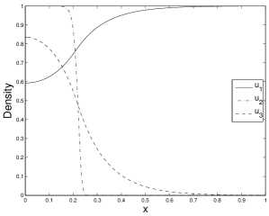
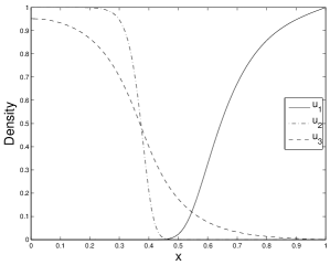
Figure 3: Density of health, tumor cells and excess concetration of H⁺ at fixed time ($t=20$) in terms of $x$ variable, for $\delta_{1}=0.5$ (left) and $\delta_{1}=12.5$ (right).

It is well-known [23] that gradient-based optimization algorithms require the evaluation of the gradient of the functional. One important advantage of evaluating the gradient through adjoints is that it requires to solve the adjoint problem only once per iteration, regardless the number of inversion variables. Note that the derivative of the functional can be approximated by using Finite Element Method.

The method we will use for minimizing the functional $\tilde{J}$ can be summarized as follows:

Algorithm 7.1

Adjoint-based minimization method.

1. Give an initial guess $\delta_{1}^{0}$ for the parameter.

2. Given $\delta_{1}^{k}$ in step $k$, solve the direct and adjoint problems at this step.

3. Obtain the derivative of the functional, i.e. $\tilde{J}^{\prime}(\delta_{1}^{k})$, using (27).

4. Obtain $\delta_{1}^{k+1}$ by performing one iteration of the SQP method.

5. Stop using the criteria of fmincon.

Algorithm 7.2

Direct problem.

1. Do an implicit Euler step to find the state variables $u$: $\displaystyle\frac{\partial u}{\partial t}(\cdot,t_{n})\approx\frac{u(\cdot,t_{n})-u(\cdot,t_{n-1})}{\tau}=F(u(\cdot,t_{n}))$, where $t_{n}=t_{n-1}+\tau$, $F(u(\cdot,t_{n}))$ is a nonlinear functional and the intial condition is $u^{0}(x)=u(x,0)$.

2. Use FEM to make a discretization of $u_{i}(x,t_{n})\approx\sum\limits_{j=1}^{nod}u^{n}_{i,j}\phi_{j}(x)$, $i=1,2,3$, $\phi_{j}(x)$ are the linear shape function and we note $U_{i}^{n}=[u^{n}_{i,1},\cdots,u^{n}_{i,j},\cdots,u^{n}_{i,nod}]\in\mathbb{R}^{nod}$, $U^{n}=[U_{1}^{n},U_{2}^{n},U_{3}^{n}]\in\mathbb{R}^{q}$, where $nod$ is the number of uniform distributed nodes for the spatial meshgrid for $[0,1]$.

3. Use the Newton method to solve: find $U^{n}\in\mathbb{R}^{q}$ such as $U^{n}-U^{n-1}-\tau G(U^{n})=0$, where $G$ is the discretization of $F$.

Algorithm 7.3

Adjoint problem.

1. Do an implicit Euler step to find the adjoint variable $\lambda$: $\displaystyle-\frac{\partial\lambda}{\partial t}(\cdot,t_{n})\approx-\frac{\lambda(\cdot,t_{n})-\lambda(\cdot,t_{n-1})}{\tau}=H(\lambda(\cdot,t_{n-1}))$, and the final condition is $\lambda(\cdot,T)=0$.

2. Use FEM to make a discretization of $\lambda(\cdot,t_{n})$ and solve the linear problem $\lambda^{n-1}-\lambda^{n}-\tau K(\lambda^{n-1})=0$, where $K$ is the discretization of $H$.

8 Numerical experiments.

The goal of this section is to test and evaluate the performance of an adjoint-based optimization method, by executing some numerical simulations of Algorithm 7.1 for some test-cases.

First consider an optimization problem that consist in minimizing the functional defined in (19), where $\hat{u}_{3}(x,t)$ is generated via the forward model, for a choice of the model parameters $\rho_{2}=1$, $D_{2}=4\times 10^{-5}$, $\delta_{3}=1$ and $\hat{\delta}_{1}=0.5,\,4,\,12.5,\,16$. We chose different values of $\hat{\delta}_{1}$ because each one of these shows a different behavior of tumor invasion, according to [7].

Figure 4 shows the value that the functional defined in (19) takes for different values of $\delta_{1}$, remaining the other parameters constant. It is worth mentioning that $\tilde{J}$ looks convex with respect to $\delta_{1}$.

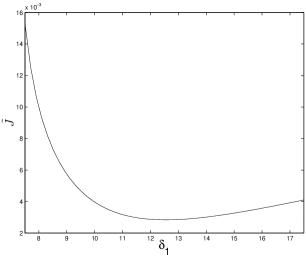
Figure 4: The functional $\tilde{J}$ for $\hat{u}_{3}$ generated with $\hat{\delta}_{1}=12.5$.

The idea of this test case is to investigate how close the original value of the parameter can be retrieved. However, it is not a trivial one, because we do not know, for instance, if the optimization problem has a solution or, in that case, if it is unique or if the method converges to another local minima.

We have run the Algorithm 7.1 for different values of $\hat{\delta}_{1}$ taking the initial condition $\delta_{1}^{0}$ randomly, as we can see from the Table 2 the retrieved parameter is obtained very accurately since the standard deviation is small. For Algorithms 7.2 and 7.3 we use the following algorithmic parameters $\tau=0.5$ and $T=20$, $nod=201$ and $U_{ad}=[0,20]$.

$\hat{\delta}_{1}$	$\bar{\delta}_{1}$	$S$
0.5	0.5000	$\pm$ 4.1372$\times 10^{-7}$
4	4.0000	$\pm$ 2.2187$\times 10^{-6}$
12.5	12.4999	$\pm$ 4.6521$\times 10^{-5}$
16	15.9993	$\pm$ 9.4495$\times 10^{-5}$

Table 2: Experiments for randomly initial data $\delta_{1}^{0}$

We emphasize that we have retrieved accurately the value of $\hat{\delta}_{1}$ independently of the value of $\delta_{1}^{0}$. Thus, in the next experiment we will consider a fixed value $\delta_{1}^{0}=8$.

It is well-known that the presence of noise in the data may imply the appearance of strong numerical instabilities in the solution of an inverse problem [24].

One of the experimental method to obtain values of $\hat{u}_{3}$ is by using fluorescence ratio imaging microscopy [8]. As it is well-known that measurements are often affected by perturbations, usually random ones.

Then we perform numerical experiments where $\hat{u}_{3}$ is perturbed by using Gaussian random noise whith mean zero and standard deviation $\sigma=0.05,\,0.1,\,0.15,\,0.2,\,0.25,\,0.3$. In the next tables 3-6, for each value of $\sigma$, we show the average $\bar{\delta}_{1}$ of 30 values of $\delta_{1}$, the standard deviation $S$ and the relative error $e_{\delta_{1}}=\frac{|\hat{\delta}_{1}-\bar{\delta}_{1}|}{\hat{\delta}_{1}}$.

$\sigma$	$\bar{\delta}_{1}$	$S$	$e_{\delta_{1}}$
0.0500	0.4707	$\pm$ 0.1231	0.0586
0.1000	0.5090	$\pm$ 0.0335	0.0180
0.1500	0.4855	$\pm$ 0.0472	0.0291
0.2000	0.4982	$\pm$ 0.0726	0.0037
0.2500	0.5112	$\pm$ 0.1022	0.0225
0.3000	0.5027	$\pm$ 0.0937	0.0054

Table 3: Experiments for $\hat{\delta}_{1}=0.5$

$\sigma$	$\bar{\delta}_{1}$	$S$	$e_{\delta_{1}}$
0.0500	4.0221	$\pm$ 0.1129	0.0055
0.1000	4.0470	$\pm$ 0.1695	0.0117
0.1500	3.9087	$\pm$ 0.2412	0.0228
0.2000	3.9459	$\pm$ 0.3524	0.0135
0.2500	3.8970	$\pm$ 0.4800	0.0258
0.3000	4.0219	$\pm$ 0.4471	0.0055

Table 4: Experiments for $\hat{\delta}_{1}=4$

$\sigma$	$\bar{\delta}_{1}$	$S$	$e_{\delta_{1}}$
0.0500	12.7922	$\pm$ 1.2354	0.0234
0.1000	13.0807	$\pm$ 1.9360	0.0465
0.1500	12.0701	$\pm$ 2.3401	0.0344
0.2000	11.4698	$\pm$ 2.7463	0.0824
0.2500	11.1943	$\pm$ 3.7566	0.1044
0.3000	11.8203	$\pm$ 4.3648	0.0544

Table 5: Experiments for $\hat{\delta}_{1}=12.5$

$\sigma$	$\bar{\delta}_{1}$	$S$	$e_{\delta_{1}}$
0.0500	16.4165	$\pm$ 2.0834	0.0261
0.1000	16.6122	$\pm$ 2.7864	0.0383
0.1500	14.8108	$\pm$ 3.3098	0.0743
0.2000	13.7965	$\pm$ 3.8915	0.1377
0.2500	14.1021	$\pm$ 4.5295	0.1186
0.3000	13.3095	$\pm$ 4.5152	0.1681

Table 6: Experiments for $\hat{\delta}_{1}=16$

Remark 8.4

Since we have used FEM to solve both Algorithms, 7.2 and 7.3, we have computed the a posteriori error in each case [25, 26]. In Table 7 we put the estimation of the a posteriori error for Algorithm 7.2 for each $\hat{\delta}_{1}$.

$\hat{\delta}_{1}$	$u_{1}$	$u_{2}$	$u_{3}$
0.5	$1.72\times 10^{-14}$	$2.43\times 10^{-10}$	$2.12\times^{-7}$
4	$1.45\times 10^{-14}$	$4.19\times 10^{-10}$	$1.80\times^{-7}$
12.5	$9.51\times 10^{-13}$	$1.12\times 10^{-9}$	$7.61\times^{-7}$
16	$5.57\times 10^{-13}$	$1.06\times 10^{-9}$	$7.61\times^{-7}$

Table 7: A posteriori error for Algorithm 7.2.

9 Final conclusions and future work.

A miscellany of new strategies, experimental techniques and theoretical approaches are emerging in the ongoing battle against cancer. Nevertheless, as new, ground-breaking discoveries relating to many and diverse areas of cancer research are made, scientists often have recourse to mathematical modelling in order to elucidate and interpret these experimental findings, [2, 4, 5, 27], and it became clear that these models are expected to success if the parameters involved in the modeling process are known. Or eventually, taking into account that some biological parameters may be unknown (especially in vivo), the model can be used to obtain them [12, 10].

This paper, as already mentioned in Section 1, aims at offering a mathematical tool for the obtention of phenomenological parameters which can be identified by inverse estimation, by making suitable comparisons with experimental data. The inverse problem was stated as a PDE-constrained optimization problem, which was solved by using the adjoint method. In addition, the gradient of the proposed functional is obtained and can be extended, in principle, to any number of unknown parameters.

We remark that the parameter estimation via PDE-constrained optimization is a general approach that can be used, for instance, to consider the effects of nonlinear interaction between the health and tumor cells [28].

As a future work we are interested in the dependence of the $\delta_{1}$ on time and in the dependence of the diffusivity coefficient of excess of the H⁺ concentration $D_{N_{3}}$ with respect to the space variable $x$, as in [29]. Also we propose to solve the problem in two dimensional space, where the importance of using adaptive FEM will be crucial.

Appendix A Appendix: obtaining the adjoint problem.

In this section we show the calculations involved in order to obtain the adjoint equations (26). As stated in Section 6, the adjoint equations constitute a weak formulation of the adjoint problem, with unknown $\zeta$, given by (21). Here, $(\frac{\partial E}{\partial u})^{*}\zeta$ is obtained by using (24). In what follows, we shall obtain equivalent expressions for each of the six terms of the summation $\langle\frac{\partial E}{\partial u}\eta,\zeta\rangle$, which are associated with the six constraints given by $E$ in (17).

$$\left\langle\frac{\partial E}{\partial u}(u,\delta_{1})\eta,\zeta\right\rangle=\lim_{\mu\rightarrow 0^{+}}\frac{\left\langle E(u+\mu\eta,\delta_{1}),\zeta\right\rangle-\left\langle E(u,\delta_{1}),\zeta\right\rangle}{\mu}.$$

$$\left\langle\frac{\partial E}{\partial u}(u,\delta_{1})\eta,\zeta\right\rangle = \int_{0}^{T}\int_{0}^{1}\left(\frac{\partial\eta_{1}}{\partial t}\lambda_{1}-\eta_{1}(1-2u_{1})\lambda_{1}+\delta_{1}\eta_{1}u_{3}\lambda_{1}+\delta_{1}u_{1}\eta_{3}\lambda_{1}\right)dxdt+$$ (28)

$$\int_{0}^{T}\int_{0}^{1}\left(\frac{\partial\eta_{2}}{\partial t}\lambda_{2}-\rho_{2}\eta_{2}(1-2u_{2})\lambda_{2}\right)dxdt+$$

$$\int_{0}^{T}\int_{0}^{1}\left(-D_{2}\eta_{1}\frac{\partial u_{2}}{\partial x}\frac{\partial\lambda_{2}}{\partial x}+D_{2}(1-u_{1})\frac{\partial\eta_{2}}{\partial x}\frac{\partial\lambda_{2}}{\partial x}\right)dxdt+$$

$$\int_{0}^{T}\int_{0}^{1}\left(\frac{\partial\eta_{3}}{\partial t}\lambda_{3}-\delta_{3}(\eta_{2}-\eta_{3})\lambda_{3}+\frac{\partial\eta_{3}}{\partial x}\frac{\partial\lambda_{3}}{\partial x}\right)dxdt+$$

$$\int_{0}^{1}\eta_{1}(x,0)\gamma_{1}dx+\int_{0}^{1}\eta_{2}(x,0)\gamma_{2}dx+\int_{0}^{1}\eta_{3}(x,0)\gamma_{3}dx,$$

using the integration by parts for time, we obtain

$$\left\langle\eta,\left(\frac{\partial E}{\partial u}(u,\delta_{1})\zeta\right)^{*}\right\rangle = \int_{0}^{T}\int_{0}^{1}\left(-\frac{\partial\lambda_{1}}{\partial t}\eta_{1}-(1-2u_{1})\lambda_{1}\eta_{1}+\delta_{1}u_{3}\lambda_{1}\eta_{1}\right)dxdt+$$ (29)

$$\int_{0}^{T}\int_{0}^{1}\left(-\frac{\partial\lambda_{2}}{\partial t}\eta_{2}-\rho_{2}(1-2u_{2})\lambda_{2}\eta_{2}-\delta_{3}\lambda_{3}\eta_{2}\right)dxdt+$$

$$\int_{0}^{T}\int_{0}^{1}\left(-D_{2}\frac{\partial u_{2}}{\partial x}\frac{\partial\lambda_{2}}{\partial x}\eta_{1}+D_{2}(1-u_{1})\frac{\partial\lambda_{2}}{\partial x}\frac{\partial\eta_{2}}{\partial x}\right)dxdt+$$

$$\int_{0}^{T}\int_{0}^{1}\left(-\frac{\partial\lambda_{3}}{\partial t}\eta_{3}+\delta_{3}\lambda_{3}\eta_{3}+\frac{\partial\lambda_{3}}{\partial x}\frac{\partial\eta_{3}}{\partial x}+\delta_{1}u_{1}\lambda_{1}\eta_{3}\right)dxdt+$$

$$\int_{0}^{1}\eta_{1}(x,0)\left(\gamma_{1}(x)-\lambda_{1}(x,0)\right)dx+\int_{0}^{1}\eta_{1}(x,T)\lambda_{1}(x,T)dx+$$

$$\int_{0}^{1}\eta_{2}(x,0)\left(\gamma_{2}(x)-\lambda_{2}(x,0)\right)dx+\int_{0}^{1}\eta_{2}(x,T)\lambda_{2}(x,T)dx+$$

$$\int_{0}^{1}\eta_{3}(x,0)\left(\gamma_{3}(x)-\lambda_{3}(x,0)\right)dx+\int_{0}^{1}\eta_{3}(x,T)\lambda_{3}(x,T)dx,$$

then choosing $\gamma(x)=\lambda(x,0)$ and $\lambda(x,T)=0$ for all $x\in[0,1]$, we obtain the following expression of $\left(\frac{\partial E}{\partial u}(u,\delta_{1})\zeta\right)^{*}$:

$$\left\langle\eta,\left(\frac{\partial E}{\partial u}(u,\delta_{1})\zeta\right)^{*}\right\rangle = \int_{0}^{T}\int_{0}^{1}\left(-\frac{\partial\lambda_{1}}{\partial t}\eta_{1}-\eta_{1}(1-2u_{1})\lambda_{1}+\delta_{1}\eta_{1}u_{3}\lambda_{1}\right)dxdt+$$ (30)

$$\int_{0}^{T}\int_{0}^{1}\left(-\frac{\partial\lambda_{2}}{\partial t}\eta_{2}-\rho_{2}\eta_{2}(1-2u_{2})\lambda_{2}-\delta_{3}\eta_{2}\lambda_{3}\right)dxdt+$$

$$\int_{0}^{T}\int_{0}^{1}\left(-D_{2}\frac{\partial u_{2}}{\partial x}\frac{\partial\lambda_{2}}{\partial x}\eta_{1}+D_{2}(1-u_{1})\frac{\partial\lambda_{2}}{\partial x}\frac{\partial\eta_{2}}{\partial x}\right)dxdt+$$

$$\int_{0}^{T}\int_{0}^{1}\left(-\frac{\partial\lambda_{3}}{\partial t}\eta_{3}+\delta_{3}\eta_{3}\lambda_{3}+\frac{\partial\lambda_{3}}{\partial x}\frac{\partial\eta_{3}}{\partial x}+\delta_{1}u_{1}\eta_{3}\lambda_{1}\right)dxdt$$

References

• Adam [1986] J. Adam, A simplified mathematical model of tumor growth, Mathematical Biosciences 81 (1986) 229–244.
• Adam and Bellomo [1997] J. Adam, N. Bellomo, A survey of models for tumor immune systems dynamics, Modeling and simulation in science, engineering & technology, Birkhäuser, 1997.
• Bellomo et al. [2009] N. Bellomo, M. Chaplain, E. De Angelis, Selected Topics on Cancer Modeling - Genesis - Evolution - Immune Competition - Therapy, Birkhäuser, Boston, 2009.
• Bellomo et al. [2008] N. Bellomo, N. Li, P. Maini, On the foundations of cancer modelling: selected topics, speculations, and perspectives, Mathematical Models and Methods in Applied Sciences 18 (2008) 593–646.
• Byrne [2010] H. M. Byrne, Dissecting cancer through mathematics: from the cell to the animal model, Nature Reviews Cancer 10 (2010) 221–230.
• Bellomo and Preziosi [2000] N. Bellomo, L. Preziosi, Modelling and mathematical problems related to tumor evolution and its interaction with the immune system, Mathematical and Computer Modelling 32 (2000) 413–452.
• Gatenby and Gawlinski [1996] R. A. Gatenby, E. T. Gawlinski, A reaction-diffusion model of cancer invasion, Cancer Research 56 (1996) 5745–5753.
• Martin and Jain [1994] G. R. Martin, R. K. Jain, Noninvasive measurement of interstitial ph profiles in normal and neoplastic tissue using fluorescence ratio imaging microscopy, Cancer research 54 (1994) 5670–5674.
• Perthame and Zubelli [2007] B. Perthame, J. Zubelli, On the inverse problem for a size-structured population model, Inverse Problems 23 (2007) 1037–1052.
• van den Doel et al. [2011] K. van den Doel, U. M. Ascher, D. K. Pai, Source localization in electromyography using the inverse potential problem, Inverse Problems 27 (2011) 025008.
• Zubelli et al. [2003] J. Zubelli, R. Marabini, C. Sorzano, G. Herman, Three-dimensional reconstruction by chahine’s method from electron microscopic projections corrupted by instrumental aberrations, Inverse Problems 19 (2003) 933–949.
• Agnelli et al. [2011] J. Agnelli, A. Barrea, C. Turner, Tumor location and parameter estimation by thermography, Mathematical and Computer Modelling 53 (2011) 1527–1534.
• Hogea et al. [2008] C. Hogea, C. Davatzikos, G. Biros, An image-driven parameter estimation problem for a reaction-diffusion glioma growth model with mass effects, J. Math. Biol. 56 (2008) 793–825.
• Knopoff et al. [2013] D. Knopoff, D. Fernández, G. Torres, C. Turner, Adjoint method for a tumour growth PDE-constrained optimization problem, Computers and Mathematics with Applications (accepted 2013).
• Ladyzhenskai︠a︡ and Solonnikov [1988] O. A. Ladyzhenskai︠a︡, V. A. Solonnikov, Linear and quasi-linear equations of parabolic type, volume 23, American Mathematical Soc., 1988.
• Kinderlehrer and Stampacchia [1987] D. Kinderlehrer, G. Stampacchia, An introduction to variational inequalities and their applications, Society for Industrial and Applied Mathematics, 1987.
• Evans [1998] L. C. Evans, Partial differential equations, American Mathematical Society, 1998.
• Gatenby et al. [2006] R. A. Gatenby, E. T. Gawlinski, A. F. Gmitro, B. Kaylor, R. J. Gillies, Acid-mediated tumor invasion: a multidisciplinary study, Cancer research 66 (2006) 5216–5223.
• Engl et al. [1996] H. W. Engl, M. Hanke, A. Neubauer, Regularization of inverse problems, volume 375, Kluwer Academic Pub, 1996.
• Kirsch [2011] A. Kirsch, An introduction to the mathematical theory of inverse problems, volume 120, Springer Science+ Business Media, 2011.
• Brandenburg et al. [2009] C. Brandenburg, F. Lindemann, M. Ulbrich, S. Ulbrich, A continuous adjoint approach to shape optimization for navier stokes flow, in: Optimal control of coupled systems of partial differential equations, Springer, 2009, pp. 35–56.
• Hinze [2009] M. Hinze, Optimization with PDE constraints, volume 23, Springer, 2009.
• Nocedal and Wright [2006] J. Nocedal, S. J. Wright, Numerical optimization, Springer Science+ Business Media, 2006.
• Bertero and Piana [2006] M. Bertero, M. Piana, Inverse problems in biomedical imaging: modeling and methods of solution, in: Complex systems in biomedicine, Springer, 2006, pp. 1–33.
• Verfürth [????] R. Verfürth, A posteriori error estimates for nonlinear problems. finite element discretizations of elliptic equations, in: 475 (1994) MR 94j:65136, p. 445.
• Babuška and Rheinboldt [1978] I. Babuška, W. C. Rheinboldt, A-posteriori error estimates for the finite element method, International Journal for Numerical Methods in Engineering 12 (1978) 1597–1615.
• Araujo and McElwain [2004] R. Araujo, D. McElwain, A history of the study of solid tumour growth: the contribution of mathematical modelling, Bulletin of mathematical biology 66 (2004) 1039–1091.
• McGillen et al. [2013] J. B. McGillen, E. A. Gaffney, N. K. Martin, P. K. Maini, A general reaction–diffusion model of acidity in cancer invasion, Journal of mathematical biology (2013) 1–26.
• Martin et al. [2010] N. K. Martin, E. A. Gaffney, R. A. Gatenby, P. K. Maini, Tumour–stromal interactions in acid-mediated invasion: a mathematical model, Journal of theoretical biology 267 (2010) 461–470.