• Local stellar kinematics from RAVE data- V. Kinematic investigation of the Galaxy with red clump stars

  S. Karaali^A,∗, S. Bilir^A, S. Ak^A, E. Yaz Gökçe^A, Ö. Önal^A, T. Ak^{A
  A} Istanbul University, Faculty of Sciences, Department of Astronomy and Space Sciences, 34119, Istanbul, Turkey
  ^∗ Email: karsa@istanbul.edu.tr

  Abstract: We investigated the space velocity components of 6610 red clump (RC) stars in terms of vertical distance, Galactocentric radial distance and Galactic longitude. Stellar velocity vectors are corrected for differential rotation of the Galaxy which is taken into account using photometric distances of RC stars. The space velocity components estimated for the sample stars above and below the Galactic plane are compatible only for the space velocity component in the direction to the Galactic rotation of the thin disc stars. The space velocity component in the direction to the Galactic rotation ($V_{lsr}$) shows a smooth variation relative to the mean Galactocentric radial distance ($R_{m}$), while it attains its maximum at the Galactic plane. The space velocity components in the Galactic centre ($U_{lsr}$) and in the vertical direction ($W_{lsr}$) show almost flat distributions relative to $R_{m}$ with small changes in their trends at $R_{m}\sim 7.5$ kpc. $U_{lsr}$ values estimated for the RC stars in quadrant $180^{o}<l\leq 270^{o}$ are larger than the ones in quadrants $0^{o}<l\leq 90^{o}$ and $270^{o}<l\leq 360^{o}$. The smooth distribution of the space velocity dispersions reveals that the thin and thick discs are kinematically continuous components of the Galaxy. Based on the $W_{lsr}$ space velocity components estimated in the quadrants $0^{o}<l\leq 90^{o}$ and $270^{o}<l\leq 360^{o}$, in the inward direction relative to the Sun, we showed that RC stars above the Galactic plane move towards the North Galactic Pole, whereas those below the Galactic plane move in the opposite direction. In the case of quadrant $180^{o}<l\leq 270^{o}$, their behaviour is different, i.e. the RC stars above and below the Galactic plane move towards the Galactic plane. We stated that the Galactic long bar is the probable origin of many, but not all, of the detected features.

  Keywords: Galaxy: kinematics and dynamics – Galaxy: solar neighbourhood – Galaxy: structure

1 Introduction

Several studies based on different techniques and data revealed the non-steady state and asymmetrical structure of our Galaxy. The Milky Way Galaxy is still evolving under the effects of internal and external forces. After the discovery of the accretion of the Sagittarius dwarf galaxy (Ibata, Gilmore & Irwin 1994), researchers drew their attention to the Galactic streams. Sagittarius stream (Majewski et al. 2003) is associated with the Sagittarius dwarf galaxy. However, there are Galactic streams whose origins are not yet known. Some of them are tidal debris and some of them originate from the accretion. Galactic warp and dynamical interaction of the thick disc with the Galactic long bar can be associated with some of the Galactic streams (Williams et al. 2013, and the references therein). The presence of some of the streams are revealed by their large-scale stellar over-densities. Monoceros stream (Newberg et al. 2002; Yanny et al. 2003) outward from the Sun and Hercules thick disc cloud (Larsen & Humphreys 1996; Parker, Humphreys & Larsen 2003, 2004; Larsen, Humphreys & Cabanela 2008) inward from the Sun are examples for these over-density structures. Helmi stream (Helmi et al. 1999) and the recent Aquarius stream (Williams et al. 2011) are also two notable streams.

Star count analysis is one of the procedures used to reveal the complex structure of the Galaxy. Bilir et al. (2006) showed that the scaleheights and the scalelengths of the thin and thick discs are Galactic longitude dependent. In Ak et al. (2007a, b), the metallicities for relatively short vertical distances ($z<2.5$ kpc) show systematic fluctuations with Galactic longitude which was interpreted as the flare effect of the disc. A more comprehensive study was carried out by Bilir et al. (2008) who showed that the thin and thick disc scaleheights as well as the axis ratio of the halo varies with Galactic longitude. The variation of these parameters were explained with the gravitational effect of the Galactic long bar. A similar work is carried out by Yaz & Karaali (2010) in intermediate latitudes of the Galaxy where the variations of the thin and thick disc scaleheights were explained with the effect of the disc flare and disc long bar.

The velocity distribution in the UV plane is also complex, i.e. it differs from a smooth Schwarzschild distribution. This has been proven for the solar neighbourhood (Dehnen 1998) and the recent studies revealed that the same case holds also for the solar suburb (Antoja et al. 2012). The complex structure is probably created by the Galactic long bar and spiral arms. Dissolving open clusters and perturbative effect of the disc by merger events can also be used for the explanation of the complexity (Williams et al. 2013). Siebert et al. (2011) showed that the radial velocities ($V_{R}$) estimated via the RAdial Velocity Experiment (RAVE; Steinmetz et al. 2006) data are non-zero and also they have a small gradient, i.e. $dV_{R}/dR<-3$ kms^-1kpc^-1. A similar result based on RAVE red clump (RC) stars has been cited in Casetti-Dinescu et al. (2011). Siebert et al. (2012) used density-wave models to show that the radial streaming originates from the resonance effect of the spiral arms, and reproduced the gradient just mentioned. Probably, the most comprehensive study is that of Williams et al. (2013) which is based on the stars from the internal release of RAVE data in October 2011. Beyond a detailed error analysis, Williams et al. (2013) confirmed the radial gradient $dV_{R}/dR<-3$ kms^-1kpc^-1 and they revealed the different behaviour of the vertical velocities, $V_{Z}$, of the RC stars in opposite regions of $R\sim 8$ kpc in the ($R$, $Z$) plane. Also, Williams et al. (2013) argued that the Hercules thick disc cloud (Larsen & Humphreys 1996; Parker et al. 2003; Larsen et al. 2008) is an important phenomenon which causes the variation of the stellar velocities. Parker et al. (2003) give the Galactic coordinates of the thick disc cloud as $20^{o}\leq l\leq 55^{o}$, $25^{o}\leq b\leq 45^{o}$, $305^{0}\leq l\leq 340^{o}$, and $-45^{o}\leq b\leq-25^{o}$. Larsen et al. (2008) stated that the center of the overdensity region ranges from ($X$, $Y$, $Z$)=(6.5, -2.2, 1.5) to ($X$, $Y$, $Z$)=(6.5, 0.3, 1.5) kpc, and that there is a clear excess of stars in quadrant $Q_{1}$ over quadrant $Q_{4}$ in the range $l=25^{o}-45^{o}$ and $b=30^{o}-40^{o}$.

In this study, we intend to contribute to the discussions of the complexity of the Milky Way Galaxy by investigating the variation of the space velocity components of 6610 RC stars. The difference between the procedures in the literature and ours is the application of a series of constraints in our work, i.e. 1) we used the space velocity components instead of the cylindrical coordinates; 2) we applied corrections for the differential rotation to our velocities; 3) we investigated the variation of the velocities for three Galactic populations, thin and thick discs, halo and their combinations; 4) we investigated the lag of the sample stars relative to the local standard of rest stars; and 5) we investigated the variation of the velocities in terms of $z_{min}$ and $z_{max}$ instead of current positions which covers the effect of long lived internal and external forces. The paper is organized as follows. The data are given in Section 2. Section 3 is devoted to the distribution of the velocity components for stars relative to several parameters: i) vertical distance, i.e. for stars above and below the Galactic plane separately, ii) Galactocentric distance, and iii) Galactic longitude. The distribution of the velocity dispersions for different velocities is also given in this section. Finally, a discussion of the results and a short conclusion is presented in Section 4.

2 Data

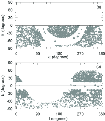
Figure 1: Distribution of RAVE DR3 RC stars in the Equatorial (a) and Galactic (b) coordinates.

The data of 6781 RC stars are taken from Bilir et al. (2012). They used the RAVE Data Release 3 (DR3, Siebert et al. 2011) survey and applied a series of constraints to 83 072 radial velocity measurements to identify 7985 RC stars among them. Also, they carried out the following evaluations to obtain the final sample of RC stars: The proper motions of 7846 stars were taken from RAVE DR3 while the 139 stars which were not available in this catalogue were provided from the PPMXL catalogue of Roeser, Demleitner & Schilbach (2010). Distances were obtained by combining the apparent $K_{S}$ magnitude of the star in question and the absolute magnitude $M_{K_{S}}=-1.54\pm 0.04$ mag, adopted for all RC stars (Groenewegen 2008), while the $E(B-V)$ reddening was obtained iteratively by using published methodology (cf. Coşkunoğlu et al. 2011, and references therein). The apparent $K_{S}$ magnitudes were de-reddened by means of the equations in Fiorucci & Munari (2003). Distribution of the RC stars in Equatorial and Galactic coordinates is given in Fig. 1.

Bilir et al. (2012) combined the distances with the RAVE DR3 radial velocities and available proper motions, applying the algorithms and transformation matrices of Johnson & Soderblom (1987) to obtain the Galactic space velocity components $(U,V,W)$ of the sample stars. In the calculations, epoch $J2000$ was adopted as described in the International Celestial Reference System of the Hipparcos and Tycho-2 catalogues (ESA 1997). The transformation matrices use the notation of right-handed system. Hence, $U$, $V$ and $W$ are the components of a velocity vector of a star with respect to the Sun, where $U$ is positive towards the Galactic center ($l=0^{o}$, $b=0^{o}$), $V$ is positive in the direction of the Galactic rotation ($l=90^{o}$, $b=0^{o}$) and $W$ is positive towards the North Galactic Pole ($b=90^{o}$).

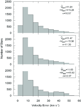
Figure 2: Distribution of the errors of the space velocity components $U$ (upper panel), $V$ (middle panel) and $W$ (lower panel) for the sample used in this study. The medians, means and the standard deviations are also stated in the panels, respectively.

Bilir et al. (2012) adopted the value of the rotation speed of the Sun as 222.5 kms^-1. Correction for differential Galactic rotation is necessary for accurate determination of the $U$, $V$ and $W$ velocity components. The effect is proportional to the projection of the distance to the stars on to the Galactic plane, i.e. the $W$ velocity component is not affected by Galactic differential rotation (Mihalas & Binney 1981). They applied the procedure of Mihalas & Binney (1981) to the distribution of the sample stars and estimated the first-order Galactic differential rotation corrections for the $U$ and $V$ velocity components of the sample stars. The $U$, $V$ and $W$ velocities were reduced to local standard of rest (LSR) by adopting the solar LSR velocities in Coşkunoğlu et al. (2011), ($U_{\odot}$, $V_{\odot}$, $W_{\odot}$)=(8.83, 14.19, 6.57) kms^-1. We will use the symbols $U_{lsr}$, $V_{lsr}$ and $W_{lsr}$ for them, hereafter. The uncertainties of the space velocities $U_{err}$, $V_{err}$ and $W_{err}$ (Fig. 2) were computed by propagating the uncertainties of the proper motions, distances and radial velocities, again using an algorithm by Johnson & Soderblom (1987). Then, the error for the total space motion of a star follows from the equation

$$S_{err}^{2}=U_{err}^{2}+V_{err}^{2}+W_{err}^{2}.$$ (1)

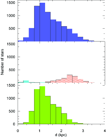
Figure 3: Distance histogram of the RC stars. Upper panel corresponds to all RC stars ($N$=7985), while the lower one is drawn for the final sample ($N$=6610). The middle panel corresponds to the RC stars with large proper motion errors ($\mu_{tot_{err}}>10$ mas yr^-1) and large distances ($d>1$ kpc, right histogram, $N$=1204), and those close to the Galactic plane ($|b|\leq 10^{o}$, left histogram, $N$=171).

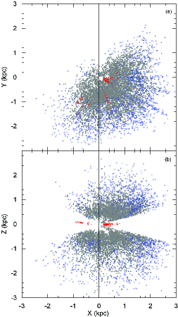
Figure 4: Distribution of the sample stars (grey colour) and rejected ones: stars with $S_{err}>75$ kms^-1 (blue colour) and stars close to the Galactic plane (red colour) in the ($X$, $Y$) and ($X$, $Z$) planes. RC stars with errors $S_{err}>75$ kms^-1 dominate the outermost region of the diagram.

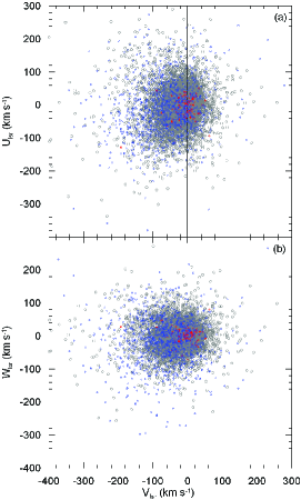
Figure 5: Distribution of the sample stars (grey colour) and rejected ones: stars with $S_{err}>75$ kms^-1 (blue colour) and stars close to the Galactic plane (red colour) in two panels of space velocity components: (a) ($V_{lsr}$, $U_{lsr}$) and (b) ($V_{lsr}$, $W_{lsr}$).

Bilir et al. (2012) removed the RC stars with total space velocity errors larger than the mean errors ($\langle S_{err}\rangle=39$ kms^-1) plus the standard deviation ($\sigma=36$ kms^-1), i.e. $S_{err}>75$ kms^-1, thus the sample reduced to 6781 stars. Also in this study, 171 RC stars that are very close to Galactic plane ($-10^{o}\leq b\leq+10^{o}$) were excluded from the sample of Bilir et al. (2012). These stars are in the calibration fields, so their properties such as age may be different from the general Galactic population we intend to study here. Thus, the final sample used in this study reduced to 6610. The large errors originate from the proper motions. The proper motions of 706 stars with $S_{err}>75$ kms^-1 is $\mu_{tot_{err}}\leq 10$ mas yr^-1 and those of 498 stars is $\mu_{tot_{err}}>10$ mas yr^-1. The distance histogram of the RC stars (Fig. 3) shows that those with large errors, $S_{err}>75$ kms^-1, locate at large distances. A proper motion error of 10 mas yr^-1 corresponds to 50 kms^-1 at 1 kpc, and correspondingly more if further away. Hence, omitting RC stars with $S_{err}>75$ kms^-1 removed the space velocity components with large errors. Also, distance and radial velocity errors may affect the space velocity components. However, in our study, they are small, i.e. distances are based on the absolute magnitude $M_{K_{s}}=-1.54\pm$0.04 mag (Groenewegen 2008), where the error is rather small, and RAVE group gives a median radial velocity error of 1.2 kms^-1 (Siebert et al. 2011). The distribution of the sample stars in the ($X$, $Y$) and ($X$, $Z$) planes and their space velocity components ($U$, $V$) and ($W$, $V$) are plotted in Fig. 4 and Fig. 5, respectively. Both figures involve the sample stars as well as the rejected ones. The RC stars with $S_{err}>75$ kms^-1 (blue colour) locate at the outermost region of Fig. 4, i.e. their $X$, $Y$ and $Z$ coordinates are larger than the sample stars (grey colour), while the RC stars close to the Galactic plane, $|b|<10^{o}$, occupy the central part of the figure, as expected. The positions of the sample stars and the stars close to the Galactic plane in Fig. 5 are almost the same as in Fig. 4. However, the stars with errors $S_{err}>75$ kms^-1 -and with large distances- are concentrated in the central part of the diagram giving the indication that their (relatively) large errors reduced their space velocity components to smaller values.

We used standard gravitational potentials described in the literature (Miyamoto & Nagai 1975; Hernquist 1990; Johnston et al. 1995; Dinescu et al. 1999) to estimate orbital elements of each of the sample stars. The orbital elements for a star used in our work are the mean of the corresponding orbital elements calculated over 15 orbital periods of that specific star. The orbital integration typically corresponds to 3 Gyr and is sufficient to evaluate the orbital elements of solar suburb stars (Coşkunoğlu et al. 2012; Bilir et al. 2012; Duran et al. 2013).

First, we performed the test-particle integration in a Milky Way potential which consists of a logarithmic halo to determine a possible orbit in the form below:

$$\Phi_{\rm halo}(r)=v_{0}^{2}\ln\left(1+\frac{r^{2}}{d^{2}}\right),$$ (2)

with $v_{0}=186$ kms^-1 and $d=12$ kpc. The disc is represented by a Miyamoto-Nagai potential (Miyamoto & Nagai 1975):

$$\Phi_{\rm disc}(R,z)=-\frac{GM_{\rm d}}{\sqrt{R^{2}+\left(a_{d}+\sqrt{z^{2}+b_{d}^{2}}\right)^{2}}},$$ (3)

with $M_{\rm d}=10^{11}~{}M_{\odot}$, $a_{d}=6.5$ kpc and $b_{d}=0.26$ kpc. Finally, the bulge is modeled as a Hernquist potential (Hernquist 1990)

$$\Phi_{\rm bulge}(r)=-\frac{GM_{\rm b}}{r+c},$$ (4)

using $M_{\rm b}=3.4\times 10^{10}~{}M_{\odot}$ and $c=0.7$ kpc. The superposition of these components gives quite a good representation of the Milky Way. The circular speed at the solar radius is 222.5 kms^-1. $P_{LSR}=2.18\times 10^{8}$ years is the orbital period of the LSR and $V_{c}=222.5$ kms^-1 denotes the circular rotational velocity at the solar Galactocentric distance, $R_{0}=8$ kpc.

For our kinematic analysis, we are interested in the mean radial Galactocentric distance ($R_{m}$) as a function of the stellar population and the orbital shape. Williams et al. (2011) have analyzed the radial orbital eccentricities of RAVE sample of thick-disc stars, to test thick-disc formation models. Here, we consider the vertical orbital eccentricity, $e_{v}$ for population analysis. $R_{m}$ is defined as the arithmetic mean of the final perigalactic ($R_{p}$) and apogalactic ($R_{a}$) distances, and $z_{max}$ and $z_{min}$ are the final maximum and minimum values of the $z$ coordinates, respectively, to the Galactic plane, where $e_{v}$ is defined as follows:

$$e_{v}=\frac{(|z_{max}|+|z_{min}|)}{R_{m}}$$ (5)

where $R_{m}=(R_{a}+R_{p})/2$ (Pauli 2005).

3 Distribution of the Space Velocity Components

3.1 Distribution of the space velocity components above and below the Galactic plane

We adopted the vertical orbital eccentricities and the procedure in Bilir et al. (2012) and separated all the sample into three populations, thin disc ($e_{v}\leq 0.12$), thick disc ($0.12<e_{v}\leq 0.25$) and halo ($e_{v}>0.25$). We carried out the same evaluation for the RC stars above and below the Galactic plane. The Galactic latitudes of these sub-samples are $b>10^{o}$ and $b<-10^{o}$, respectively, due to the restriction explained in Section 2. The space velocity components and their corresponding dispersions for three categories are given in Table 1. The number of stars for the thin disc are in majority, while those for the halo are in minority, as expected for a sample of stars in the solar suburb. The data confirm another expectation of us, i.e. the numerical values for a specific velocity component are different for different populations. One can see in Table 1 that there is a symmetrical distribution relative to the Galactic plane for only two parameters, i.e. the space velocity component $V_{lsr}$ and its total dispersion $\sigma_{tot}$. The number of stars below the Galactic plane is larger than the ones above, due to the observational strategy of RAVE, 3801 and 2809 stars respectively. Hence, the errors of the space velocity components for the stars with $b<-10^{o}$ are less than the corresponding ones with $b>10^{o}$.

3.2 Distribution of the space velocity components relative to the Galactocentric radial distance in different $z_{min}$ and $z_{max}$ intervals

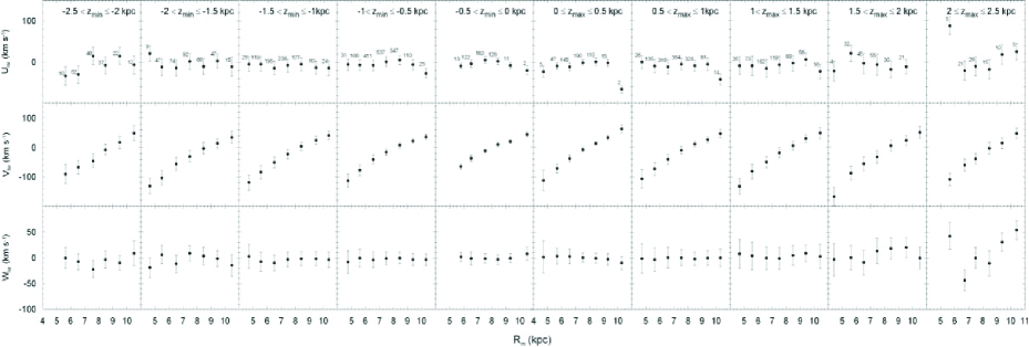
Figure 6: Distribution of the space velocity components relative to the LSR velocities, $U_{lsr}$, $V_{lsr}$, $W_{lsr}$, in terms of mean Galactocentric radial distance $R_{m}$, for five $z_{min}$ and five $z_{max}$ intervals. The figures at the top panel indicate the number of stars. The error bars are also shown in the diagram.

We estimated the space velocity components of the sample stars relative to $R_{m}$ in different $z_{min}$ and $z_{max}$ intervals. The ranges of these parameters are $4<R_{m}\leq 11$, $-2.5\leq z_{min}\leq 0$ and $0<z_{max}\leq 2.5$ kpc. The results are given in Table 2. The distributions of the space velocity components are given in Fig. 6. In the following, we discuss the trends in each space velocity component.

3.2.1 $U_{lsr}$

The variation of the space velocity component $U_{lsr}$ is given at the top panel of Fig. 6. When we consider the errors, the general trend is a flat distribution. However, there are different distributions in some $z_{min}$/$z_{max}$ intervals, such as $-1<z_{min}\leq-0.5$ and $-0.5<z_{min}\leq 0$ kpc where a small increase in $U_{lsr}$ can be detected at $\sim$7.5 kpc. Whereas, the numerical value of $U_{lsr}$ in the interval $1.5<z_{max}\leq 2$ kpc at distance $R_{m}\sim 7.5$ kpc give the indication of a change in the trend, i.e. the decreasing velocity component in the distance interval $5<R_{m}<7.5$ kpc flattens at larger $R_{m}$ distances. A different figure is related to the extreme intervals, $-2.5\leq z_{min}\leq-2$ and $2<z_{max}\leq 2.5$ kpc, where $U_{lsr}$ is an increasing function of $R_{m}$. However, the number of stars in these intervals are small.

3.2.2 $V_{lsr}$

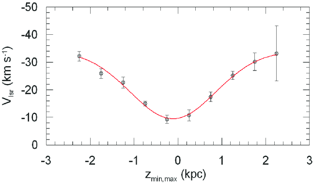
Figure 7: Diagram of the mean $V_{lsr}$ space velocity components for five $z_{min}$ and five $z_{max}$ distances. The error bars are also shown in the diagram.

The middle panel in Fig. 6 shows that there is a smooth variation of the velocity component $V_{lsr}$ with respect to $R_{m}$ for all $z_{min}$ and $z_{max}$ intervals. Also, there is a slight indication (at least for the smallest values in each interval) that $V_{lsr}$ values for the RC stars for $b<-10^{o}$ increases with decreasing distance to the Galactic plane, while they increase gradually with increasing distance to the Galactic plane for $b>10^{o}$. This argument has been confirmed by the mean of $V_{lsr}$ velocity components in $z_{min}$ and $z_{max}$ intervals. Fig. 7 shows that there is almost a symmetrical distribution of the mean $V_{lsr}$ velocity components with respect to $z_{min}$ and $z_{max}$ for all RC stars. That is the $V_{lsr}$ velocity component values are highest in the Galactic plane and they become relatively lower with higher Galactic latitudes. This is what we expect from the Jeans equations, $V_{lsr}$ decreases as the asymmetrical drift increases and asymmetric drift increases with velocity dispersion (cf. Binney & Tremaine 1998). The symmetric shape of the curve in this figure is also a general property of stellar Galactic orbits, i.e. $z_{min}\approx-z_{max}$, due to symmetry of the Galactic potential relative to the Galactic plane.

3.2.3 $W_{lsr}$

The distribution of the space velocity component $W_{lsr}$ is given in the lower panel of Fig. 6. The distribution is rather flat in all $z_{min}$ and $z_{max}$ intervals, except in the intervals $-2.5\leq z_{min}\leq-2$ and $1.5<z_{max}\leq 2$ kpc where in the first interval there is a concave shape with a minimum at $\sim$7.5 kpc and where there is an extended peak covering the Galactocentric distances larger than $R_{m}\sim 7.5$ kpc following the flat distribution in shorter distances, $R_{m}\leq 7.5$ kpc. While $W_{lsr}$ increases with $R_{m}$ distance monotonously in the interval $2<z_{max}\leq 2.5$ kpc. We omit the first bin in this interval which contains only five stars.

3.3 Distribution of the space velocity components relative to the Galactic longitude in different $z_{min}$ and $z_{max}$ intervals

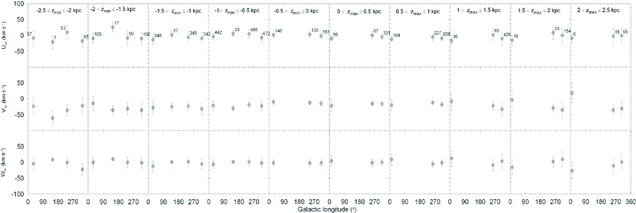
Figure 8: Distribution of the space velocity components relative to the LSR velocities, $U_{lsr}$, $V_{lsr}$, $W_{lsr}$, in terms of Galactic longitude, for five $z_{min}$ and five $z_{max}$ intervals. The figures at the top panel indicate the number of stars. The error bars are also shown in the diagram.

In this section, we discuss the distribution of the space velocity components relative to the Galactic longitude. However, we stress that we can not discuss motions in all four quadrants on equal footing, as RAVE observed only stars in the southern celestial hemisphere. We evaluated the mean of the space velocity components $U_{lsr}$, $V_{lsr}$ and $W_{lsr}$, for four quadrants, $Q_{1}(0^{o}\leq l\leq 90^{o})$, $Q_{2}(90^{o}<l\leq 180^{o})$, $Q_{3}(180^{o}<l\leq 270^{o})$ and $Q_{4}(270^{o}<l\leq 360^{o})$ of the Galaxy (Table 3) and plotted them in Fig. 8. We discuss the most striking features of the space velocity components in the following.

3.3.1 $U_{lsr}$

Distribution of the $U_{lsr}$ space velocity components relative to the quadrants are plotted at the top panel in Fig. 8. Two features can be detected in $z_{min}$ and $z_{max}$ intervals: i) There are systematic differences between the space velocity components in the quadrants $Q_{1}$, $Q_{3}$ and $Q_{4}$, $U_{lsr}$ being larger in $Q_{3}$ than ones in $Q_{1}$ and $Q_{4}$ in all $z_{min}$ and $z_{max}$ intervals, except $2<z_{max}\leq 2.5$ kpc. ii) The $U_{lsr}$ space velocity component corresponding the data in $Q_{1}$ decreases monotonously with increasing distance to the Galactic plane in the ranges $-1.5<z_{min}\leq 0$ and $0<z_{max}\leq 1.5$ kpc and it increases at relatively extreme distances.

3.3.2 $V_{lsr}$

The middle panel of Fig. 8 shows that, for $z_{min}$ intervals, the $V_{lsr}$ space velocity component for a given $Q_{i}$ ($i$=1, 3, 4) increases with increasing $z_{min}$, i.e. a result stated in Section 3.2.1. That is the $V_{lsr}$ space velocity components attain their larger values at lower Galactic latitudes. Any numerical value of $V_{lsr}$ which does not obey to this argument is related to the number of stars used for its evaluation and consequently its error. As an example, we give the $V_{lsr}$ values and the number of stars for the intervals $-1.5<z_{min}\leq-1$, $-2<z_{min}\leq-1.5$, and $-2.5\leq z_{min}\leq-2$ kpc, for the quadrant $Q_{1}$, i.e. $V_{lsr}=-27.7\pm 20.08$ kms^-1, $N=246$; $V_{lsr}=-14.54\pm 22.62$ kms^-1, $N=103$; and $V_{lsr}=-23.32\pm 27.12$ kms^-1, $N=57$, respectively. The numerical value of $V_{lsr}$ for the first $z_{min}$ interval obeys the argument just cited, whereas those for the other two $z_{min}$ intervals with higher errors and less number of stars do not. For $z_{max}$ intervals, the same case holds only for the $Q_{3}$ and $Q_{4}$, while the behaviour of the $V_{lsr}$ space velocity component for $Q_{1}$ is in opposite sense. We can not consider the $V_{lsr}$ space velocity component for $Q_{2}$ due to absence of stars for this quadrant.

3.3.3 $W_{lsr}$

Distribution of the $W_{lsr}$ space velocity components relative to the quadrants are plotted in the lower panel of Fig. 8. The behaviours of $W_{lsr}$ for stars in two quadrants are rather interesting. In $Q_{1}$, $W_{lsr}$ is positive in three $z_{max}$ intervals, $0<z_{max}\leq 0.5$, $0.5<z_{max}\leq 1$, and $1<z_{max}\leq 1.5$ kpc, while it is negative in all five $z_{min}$ intervals. That is, the RC stars above the Galactic plane in $Q_{1}$ move towards the direction of North Galactic Pole, whereas those below the Galactic plane in the same quadrant move in the opposite direction. The number of stars in the intervals $1.5<z_{max}\leq 2$ and $2<z_{max}\leq 2.5$ kpc which do not obey the argument just stated are only N=16 and 6, respectively. However, the case is reverse for the RC stars in quadrant $Q_{3}$, i.e. $W_{lsr}$ is negative in the same $z_{max}$ intervals, $0<z_{max}\leq 0.5$, $0.5<z_{max}\leq 1$, and $1<z_{max}\leq 1.5$ kpc, while it is positive in three $z_{min}$ intervals: $-2<z_{min}\leq-1.5$, $-1.5<z_{min}\leq-1$, $-1<z_{min}\leq-0.5$ kpc. That is, the RC stars above and below the Galactic plane in the $z_{max}$ and $z_{min}$ intervals cited move towards the Galactic plane.

The errors of the $U_{lsr}$ and $W_{lsr}$ are larger than the absolute values of the corresponding space velocities. Hence, the behaviours of these velocity components are probably more complicated than we detected. RAVE observed only stars in the southern celestial hemisphere. Hence, the number of stars with $z_{max}$ distances are relatively smaller than the corresponding ones with $z_{min}$ ones which causes larger errors.

3.4 Distribution of the space velocity dispersions

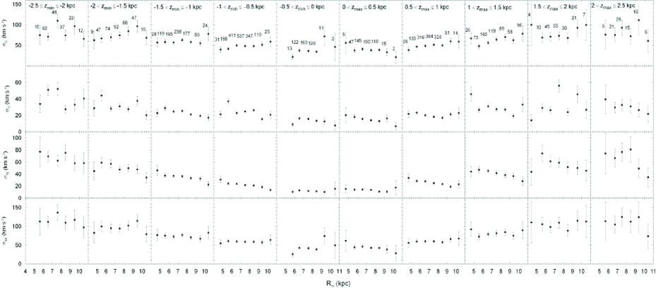
Figure 9: Distribution of the dispersions of space velocity components relative to the LSR velocities, $\sigma_{U}$, $\sigma_{V}$, $\sigma_{W}$, $\sigma_{tot}$, in terms of mean Galactocentric radial distance $R_{m}$, for five $z_{min}$ and five $z_{max}$ intervals. The figures at the top panel indicate the number of stars. The error bars are also shown in the diagram.

We estimated the dispersions of the space velocity components for the sample stars as a function of $R_{m}$ in different $z_{min}$ and $z_{max}$ intervals. The ranges of $R_{m}$, $z_{min}$ and $z_{max}$ are $4\leq R_{m}\leq 11$, ${-2.5}\leq z_{min}\leq 0$ and $0<z_{max}\leq 2.5$ kpc, respectively. The results are given in Table 2 and Fig. 9. The RC stars at extreme Galactocentric distances, $4\leq R_{m}\leq 5$ and $10<R_{m}\leq 11$ kpc, are small in number. The number of stars are also relatively small for ${-2.5}\leq z_{min}\leq{-2}$ and $2<z_{max}\leq 2.5$ kpc intervals, and their errors are large. In our discussions below, we will give less weight to the bins corresponding to small number of stars and relatively large errors.

The distribution of the $\sigma_{U}$ dispersion is almost flat in ${-0.5}<z_{min}\leq 0$ and $0<z_{max}\leq 0.5$ kpc intervals, while there is a positive (but small) gradient in other $z_{min}$ and $z_{max}$ intervals, i.e. $\sigma_{U}$ increases with increasing $R_{m}$. That is, the distribution of $\sigma_{U}$ is different between the ranges close to the Galactic plane and the further ones.

The distribution of the $\sigma_{V}$ dispersion is also flat in ${-0.5}<z_{min}\leq 0$ and $0<z_{max}\leq 0.5$ kpc intervals. However, one can detect a small gradient in some of the other $z_{min}$ and $z_{max}$ intervals, such as ${-1.5}<z_{min}\leq{-1}$ and ${0.5}<z_{max}\leq{1}$kpc.

The trend of the distribution of the dispersion $\sigma_{W}$ is almost the same as $\sigma_{U}$ and $\sigma_{V}$ in the intervals ${-0.5}<z_{min}\leq 0$ and $0<z_{max}\leq 0.5$ kpc, while there is a gradient in the distribution of $\sigma_{W}$ in the other $z_{min}$ and $z_{max}$ intervals. Additionally, this gradient is in opposite sense cited for $\sigma_{U}$ velocity dispersion , i.e. $\sigma_{W}$ decreases with increasing $R_{m}$ distance.

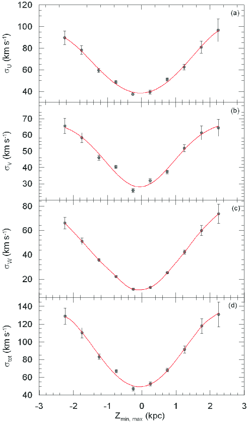
Figure 10: Mean dispersions of the space velocity components, $\sigma_{U}$, $\sigma_{V}$, $\sigma_{W}$ and $\sigma_{tot}$, for five $z_{min}$ and five $z_{max}$ intervals.

The general aspect of the distribution of each space velocity dispersion, $\sigma_{U}$, $\sigma_{V}$, $\sigma_{W}$ and $\sigma_{tot}$, in Fig. 9 gives the indication of a parabolic function with its vertex at the Galactic plane: the space velocity dispersions are small in two intervals, ${-0.5}<z_{min}\leq 0$ and $0<z_{max}\leq 0.5$ kpc, but gradually, they become larger in the $z_{min}$ and $z_{max}$ intervals correspond to a larger distances from the Galactic plane. The small gradients in the $z_{min}$ and $z_{max}$ intervals encouraged us to estimate the mean space velocity dispersion in these intervals and plotted them versus corresponding mean $z_{min}$ and $z_{max}$ values. Fig. 10 shows that a Gaussian distribution fits to each of the space velocity dispersion, i.e. $\sigma_{U}$, $\sigma_{V}$, $\sigma_{W}$, $\sigma_{tot}$. Also, the smooth distribution of the velocity dispersions reveals that the thin and thick discs are kinematically continuous components of the Galaxy. Actually, the majority of our sample consists of the thin and thick discs RC stars, and there is a smooth transition between the small (thin disc) and relatively large (thick disc) space velocity dispersion in Fig. 10. As stated in Section 3.2.2, the symmetric shapes of the curves in this figure is also a general property of stellar Galactic orbits, i.e. $z_{min}\approx-z_{max}$, and the symmetric of the Galactic potential relative to the Galactic plane.

4 Summary and Discussion

We used the space velocity components and their dispersions of 6610 RC stars and investigated their distribution relative to vertical distance, Galactocentric radial distance and Galactic longitude. The total error of the space velocity components is restricted with $S_{err}\leq 75$ kms^-1, and space velocity components are corrected with differential rotation, to obtain reliable data. Also, we investigated the variation of the space velocity components in terms of $z_{min}$ and $z_{max}$ distances instead of $z$ which covers the effect of long lived internal and external forces.

In our distance calculations, we adopted a single value of absolute value, $M_{K_{S}}=-1.54$ mag (Groenewegen 2008). It has been cited in the literature (cf. Williams et al. 2013) that the use of a single value does not compromise the results considerably. The proper motions of all RC stars are taken from RAVE DR3, except those of 139 stars which were not available in this catalogue and which were provided from the PPMXL, as cited in Section 2. Different proper motion catalogues such as SPM4 and UCAC3 could be used as well. However, different proper motions change only the predicted values of the space velocity components but not the trends of their distributions. Additionally, the difference between the values of a given space velocity component predicted by two different proper motion catalogue is not large (cf. Williams et al. 2013). We omitted the RC stars with total error $S_{err}>75$ kms^-1 in their space velocities where most of these errors originate from the proper motions. The proper motions of 706 stars with $S_{err}>75$ kms^-1 is $\mu_{tot_{err}}\leq 10$ mas and those of 498 stars is $\mu_{tot_{err}}>10$ mas. The distances are based on a single absolute magnitude with an error of $\pm 0.04$ mag, and RAVE group gives a median radial velocity error of 1.2 kms^-1 (Siebert et al. 2011). Hence, the effect of the distance errors and radial velocity should be much smaller than the one for proper motion.

The space velocity components and their dispersions for different populations, i.e. thin and thick discs and halo, are different as expected. The space velocity components for RC stars above ($b>10^{o}$) and below ($b<-10^{o}$) the Galactic plane are compatible only for $V_{lsr}$ of the thin disc.

The $V_{lsr}$ space velocity component is vertical distance ($z_{min}$ and $z_{max}$) and $R_{m}$ dependent. There is a smooth variation relative to $R_{m}$. The mean of the $V_{lsr}$ space velocity components for 10 $z_{min}$ and $z_{max}$ intervals could be fitted to a Gaussian distribution with a minimum point at the Galactic plane, a result expected from the Jeans equations, i.e. $V_{lsr}$ decreases as the asymmetric drift increases and asymmetric drift increases with space velocity dispersion (Binney & Tremaine 1998).

The general trend of the space velocity component $U_{lsr}$ is a flat distribution in terms of $R_{m}$ for most of the $z_{min}$ and $z_{max}$ intervals. However, there are some intervals where the trend changes at $\sim$7.5 kpc. Also, the distribution in the extreme intervals, ${-2.5}\leq z_{min}\leq{-2}$ and $2<z_{max}\leq 2.5$ kpc is an increasing function. However, the number of stars in these intervals are relatively small corresponding to larger errors.

The distribution of the space velocity component $W_{lsr}$ is also flat, again with some exceptions, i.e. there is a concave shape with a minimum at $R_{m}\sim 7.5$ kpc in the interval $-2.5\leq z_{min}\leq-2$ kpc, and an extended peak covering distances larger than $R_{m}\sim 7.5$ kpc, following the flat distribution in shorter distances. The distribution of $W_{lsr}$ is an increasing function in the extreme interval, $2<z_{max}\leq 2.5$, similar to $U_{lsr}$.

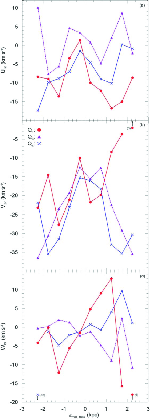
Figure 11: Distribution of the space velocity components relative to the LSR velocities, $U_{lsr}$, $V_{lsr}$, $W_{lsr}$, for three quadrants: $Q_{1}(0^{o}\leq l\leq 90^{o})$, $Q_{3}(180^{o}<l\leq 270^{o})$ and $Q_{4}(270^{o}<l\leq 360^{o})$ shown with different symbols, in terms of for five $z_{min}$ and five $z_{max}$ distances. Figures in the parenthesis indicate the (small) number of stars for which the errors are large.

The behaviours of the space velocity components are different in four quadrants (Fig. 11). The upper panel of Fig. 11 shows that the space velocity components $U_{lsr}$ estimated for the RC stars in the quadrant $Q_{3}$ ($180^{o}<l\leq 270^{o}$) are larger than the ones estimated for the RC stars in quadrants $Q_{1}$ ($0^{o}\leq l\leq 90^{o}$) and $Q_{4}$ ($270^{o}<l\leq 360^{o}$) for all $z_{min}$ and $z_{max}$ intervals, except the interval $2<z_{max}\leq 2.5$ kpc which is not valid for $Q_{4}$. We will see in the following that $z_{min}$ and $z_{max}$ intervals which involves small number of stars, such as in the present case where the number of stars is only $N=15$, show exceptions due to corresponding large errors. Different $U_{lsr}$ space velocity components indicates different lag for the RC stars in different quadrants. The $U_{lsr}$ velocity components for quadrants $Q_{1}$ and $Q_{4}$ attain their maximum values at small distances to the Galactic plane, while its distribution for the quadrant $Q_{3}$ gives the indication of a double peak distribution. In our analysis, we give less weight to the (relatively) extreme $z_{min}$ and $z_{max}$ intervals due to larger errors, as mentioned above in this paragraph.

The space velocity component $V_{lsr}$ shows almost a similar distribution in terms of $z_{min}$ and $z_{max}$ distances in the quadrants $Q_{3}$ and $Q_{4}$ (middle panel), i.e. $V_{lsr}$ attains its (relative algebraic) large numerical values in $-0.5<z_{min}\leq 0$ and $0<z_{max}\leq 1$ kpc intervals, then it decreases gradually with larger distances from the Galactic plane. That is, the lag for the space velocity component in the direction to the Galactic rotation increases from the Galactic plane to larger vertical distances. However, the same case does not hold for $V_{lsr}$ estimated for the RC stars in the quadrant $Q_{1}$, i.e. the distribution of $V_{lsr}$ shows two minima and three maxima in the interval formed by combining five $z_{min}$ and five $z_{max}$ intervals. Especially, $V_{lsr}$ is a monotonous increasing function in the $z_{max}$ intervals, starting from a minimum point in $0<z_{max}\leq 0.5$ kpc interval which also contradicts with the maximum $V_{lsr}$ space velocity components estimated in the quadrants $Q_{3}$ and $Q_{4}$.

In the case of the space velocity component $W_{lsr}$, the similarity exists for the RC stars in the quadrants $Q_{1}$ and $Q_{4}$, as explained in the following. The numerical values of $W_{lsr}$ for the quadrants $Q_{1}$ and $Q_{4}$ are negative for all $z_{min}$ intervals, while they are positive for $Q_{1}$ in three $z_{max}$ intervals, $0<z_{max}\leq 0.5$, $0.5<z_{max}\leq 1$, and $1<z_{max}\leq 1.5$ kpc. However, the number of stars in the other two $z_{max}$ intervals where $W_{lsr}$ is not positive, are only 16, and 6. $W_{lsr}$ is positive for $Q_{4}$ for four $z_{max}$ intervals, and its numerical value in the fifth $z_{max}$ interval, $0.5<z_{max}\leq 1$ kpc, is only -0.73 kms^-1. The overall picture for the space velocity component in the quadrants $Q_{1}$ and $Q_{4}$ (in the inward direction relative to the Sun) is that RC stars above the Galactic plane move in the direction to the North Galactic Pole, whereas those below the Galactic plane move in the opposite direction, they show a rarefaction. The distribution of the space velocity component $W_{lsr}$ in the quadrant $Q_{3}$ is different than the ones in the quadrants $Q_{1}$ and $Q_{4}$, i.e. $W_{lsr}$ is positive (or close to zero) in four $z_{min}$ intervals and negative in four $z_{max}$ intervals. That is, in the case of quadrant $Q_{3}$ (in the outward direction), RC stars above and below the Galactic plane move towards the Galactic plane, they show a compression. We could not consider the quadrant $Q_{2}$ due to absence of stars in the $z_{max}$ intervals and only 94 stars in the $z_{min}$ intervals. Also, we stress (again) that we can not discuss motions in three quadrants on equal footing, as RAVE observed only stars in the southern celestial hemisphere.

Our results confirm the complex structure of our Galaxy. It is non-homogeneous, non-steady state, and asymmetric. The rarefaction and the compression of the RC stars in different quadrants were detected also in Williams et al. (2013). However, their procedure is different. In Williams et al. (2013), two opposite features were based on the Galactocentric radial distance, i.e. inward of $R_{o}=8.5$ kpc stars show a rarefaction, while outward of $R_{o}$ kpc they show a compression. In Bilir et al. (2008), the Galactic longitude dependence of the scaleheights of the thin and thick discs were explained with the gravitational effect of the Galactic long bar (see also, Cabrera-Lavers et al. 2007). Hence, the features detected in our study probably originate from the Galactic long bar, rather than any other event such as an accretion. The vertical distances, $z_{min}$ and $z_{max}$, used in this study correspond to a long lived time scale. Hence, any event related to the gradients of the space velocity components should be also long lived. Also this argument favors the Galactic long bar.

However, we do not argue that all the features mentioned above can be explained with only one event. Differences between the lags for the $U_{lsr}$ space velocity components of the stars at the same vertical distance but in different quadrants, such as $Q_{1}$, $Q_{3}$ and $Q_{4}$, need alternative events.

Conclusion: The distributions of the space velocity components $U_{lsr}$, $V_{lsr}$, and $W_{lsr}$, relative to the vertical distance $z_{max}/z_{min}$, Galactocentric distance $R$, and Galactic longitude $l$ show that the Milky Way Galaxy has a non-homogeneous, non-steady state and asymmetric structure. The Galactic long bar is the probable origin of many, but not all, of the features detected.

5 Acknowledgments

We are grateful to the anonymous reviewer who improved our paper by his/her comments and suggestions.This work has been supported in part by the Scientific and Technological Research Council (TÜBİTAK) 112T120. Funding for RAVE has been provided by: the Australian Astronomical Observatory; the Leibniz-Institut fuer Astrophysik Potsdam (AIP); the Australian National University; the Australian Research Council; the French National Research Agency; the German Research Foundation; the European Research Council (ERC-StG 240271 Galactica); the Istituto Nazionale di Astrofisica at Padova; The Johns Hopkins University; the National Science Foundation of the USA (AST-0908326); the W. M. Keck foundation; the Macquarie University; the Netherlands Research School for Astronomy; the Natural Sciences and Engineering Research Council of Canada; the Slovenian Research Agency; the Swiss National Science Foundation; the Science & Technology Facilities Council of the UK; Opticon; Strasbourg Observatory; and the Universities of Groningen, Heidelberg and Sydney. The RAVE web site is at
http://www.rave-survey.org

This publication makes use of data products from the Two Micron All Sky Survey, which is a joint project of the University of Massachusetts and the Infrared Processing and Analysis Center/California Institute of Technology, funded by the National Aeronautics and Space Administration and the National Science Foundation. This research has made use of the SIMBAD, NASA’s Astrophysics Data System Bibliographic Services and the NASA/IPAC ExtraGalactic Database (NED) which is operated by the Jet Propulsion Laboratory, California Institute of Technology, under contract with the National Aeronautics and Space Administration.

Table 1: The space velocity components relative to the LSR velocities ($U_{lsr}$, $V_{lsr}$, $W_{lsr}$) and their dispersions ($\sigma_{U}$, $\sigma_{V}$, $\sigma_{W}$, $\sigma_{tot}$), for the RC stars above ($b>10^{o}$) and below ($b<-10^{o}$) the Galactic plane in terms of vertical eccentricity $e_{v}$. $N$ denotes the number of stars and, $\sigma_{tot}$ is the total space velocity dispersion. The errors of the space velocity components are the mean of the errors of the corresponding stars, while those for the dispersions are the standard errors.

RC Sample	$e_{v}$	$N$	$<U_{lsr}>$	$<V_{lsr}>$	$<W_{lsr}>$	$\sigma_{U}$	$\sigma_{V}$	$\sigma_{W}$	$\sigma_{tot}$
			(kms-1)	(kms-1)	(kms-1)	(kms-1)	(kms-1)	(kms-1)	(kms-1)
All	[0, 0.12]	3283	-3.16$\pm$11.58	-9.47$\pm$10.92	-0.69$\pm$13.35	47.55$\pm$0.83	32.81$\pm$0.57	19.55$\pm$0.34	60.99$\pm$1.06
	(0.12, 0.25]	2387	-8.46$\pm$17.55	-29.56$\pm$18.20	-1.16$\pm$17.92	62.68$\pm$1.28	50.22$\pm$1.03	38.89$\pm$0.80	89.24$\pm$1.83
	(0.25, 1]	940	-2.80$\pm$22.45	-71.36$\pm$23.84	-2.16$\pm$19.86	93.33$\pm$3.04	82.51$\pm$2.69	88.73$\pm$2.89	152.94$\pm$4.99
$b>10^{o}$	[0,0.12]	1550	-6.65$\pm$11.99	-9.10$\pm$11.22	0.49$\pm$14.20	48.96$\pm$1.24	32.31$\pm$0.82	20.46$\pm$0.52	62.13$\pm$1.58
	(0.12, 0.25]	929	-7.53$\pm$20.23	-32.71$\pm$19.75	2.15$\pm$22.21	63.33$\pm$2.08	52.56$\pm$1.72	41.42$\pm$1.36	92.14$\pm$3.02
	(0.25, 1]	330	2.18$\pm$23.11	-67.24$\pm$22.59	4.76$\pm$23.15	98.04$\pm$5.40	85.17$\pm$4.69	98.32$\pm$5.41	162.89$\pm$8.97
$b<-10^{o}$	[0, 0.12]	1733	-0.05$\pm$11.22	-9.80$\pm$10.65	-1.74$\pm$12.58	46.06$\pm$1.11	33.25$\pm$0.80	18.63$\pm$0.45	59.78$\pm$1.44
	(0.12, 0.25]	1458	-9.05$\pm$15.85	-27.56$\pm$17.20	-3.26$\pm$15.19	62.27$\pm$1.63	48.59$\pm$1.27	37.04$\pm$0.97	87.24$\pm$2.28
	(0.25, 1]	610	-5.50$\pm$22.10	-73.59$\pm$24.52	-5.90$\pm$18.08	90.64$\pm$3.67	81.03$\pm$3.28	82.94$\pm$3.36	147.18$\pm$5.96

Table 2: The space velocity components relative to the LSR velocities ($U_{lsr}$, $V_{lsr}$, $W_{lsr}$) and their space velocity dispersions ($\sigma_{U}$, $\sigma_{V}$, $\sigma_{W}$, $\sigma_{tot}$) for the RC stars in terms of mean Galactocentric radial distance ($R_{m}$) for five $z_{min}$ and five $z_{max}$ intervals. $N$ denotes the number of RC stars in the $R_{m}$ range stated on the same line. Errors as defined in Table 1.

$z_{min}$/$z_{max}$	$R_{m}$ Range	$R_{m}$	$N$	$<U_{lsr}>$	$<V_{lsr}>$	$<W_{lsr}>$	$\sigma_{U}$	$\sigma_{V}$	$\sigma_{W}$	$\sigma_{tot}$
(kpc)	(kpc)	(kpc)		(kms-1)	(kms-1)	(kms-1)	(kms-1)	(kms-1)	(kms-1)	(kms-1)
(2, 2.5]	(5, 6]	5.65	5	87.75$\pm$21.54	-109.10$\pm$21.14	42.48$\pm$25.49	76.37$\pm$34.15	39.45$\pm$17.64	74.49$\pm$33.31	113.74$\pm$50.87
	(6, 7]	6.72	21	-20.70$\pm$23.23	-59.97$\pm$20.72	-43.58$\pm$20.21	75.35$\pm$16.44	29.47$\pm$6.43	66.43$\pm$14.50	104.69$\pm$22.85
	(7, 8]	7.49	26	-10.28$\pm$22.87	-38.39$\pm$18.05	0.04$\pm$20.08	93.01$\pm$18.24	32.58$\pm$6.39	76.79$\pm$15.06	124.94$\pm$24.50
	(8, 9]	8.47	15	-17.38$\pm$23.26	-2.93$\pm$20.96	-10.69$\pm$24.03	72.31$\pm$18.67	30.82$\pm$7.96	80.87$\pm$20.88	112.78$\pm$29.12
	(9, 10]	9.38	10	18.52$\pm$24.06	13.91$\pm$18.27	31.05$\pm$17.87	111.28$\pm$35.19	26.55$\pm$8.40	49.30$\pm$15.59	124.57$\pm$39.39
	10, 11]	10.42	5	25.33$\pm$19.93	47.42$\pm$17.32	54.09$\pm$17.97	61.00$\pm$27.28	21.66$\pm$9.69	34.49$\pm$15.42	73.35$\pm$32.80
(1.5, 2]	(4, 5]	4.40	4	-21.85$\pm$24.20	-167.26$\pm$31.43	-3.21$\pm$31.57	100.24$\pm$50.12	14.10$\pm$7.05	43.76$\pm$21.88	110.28$\pm$55.14
	(5, 6]	5.61	32	21.28$\pm$19.59	-87.49$\pm$23.86	0.82$\pm$23.30	69.03$\pm$12.20	28.99$\pm$5.12	74.33$\pm$13.14	105.50$\pm$18.65
	(6, 7]	6.53	45	-3.31$\pm$24.62	-55.30$\pm$23.98	-9.15$\pm$24.30	71.31$\pm$10.63	26.23$\pm$3.91	61.53$\pm$9.17	97.77$\pm$14.57
	(7, 8]	7.48	55	-6.42$\pm$26.03	-32.82$\pm$20.83	13.27$\pm$24.86	73.20$\pm$9.87	56.06$\pm$7.56	59.11$\pm$7.97	109.52$\pm$14.77
	(8, 9]	8.45	30	-17.49$\pm$20.53	6.28$\pm$19.52	18.22$\pm$20.73	67.86$\pm$12.39	23.99$\pm$4.38	51.57$\pm$9.42	88.54$\pm$16.17
	(9, 10]	9.53	21	-11.06$\pm$17.06	23.68$\pm$16.98	20.10$\pm$19.22	92.66$\pm$20.22	45.67$\pm$9.97	50.23$\pm$10.96	114.87$\pm$25.07
	(10, 11]	10.51	7	50.08$\pm$22.16	50.89$\pm$19.59	0.13$\pm$21.06	99.80$\pm$37.72	26.72$\pm$10.10	45.85$\pm$17.33	113.03$\pm$42.72
(1, 1.5]	(4, 5]	4.68	26	-9.09$\pm$21.74	-132.42$\pm$27.69	7.97$\pm$28.03	66.87$\pm$13.11	45.85$\pm$8.99	44.11$\pm$8.65	92.30$\pm$18.10
	(5, 6]	5.57	73	-9.22$\pm$23.60	-81.78$\pm$25.03	4.13$\pm$26.89	48.12$\pm$5.63	26.82$\pm$3.14	47.25$\pm$5.53	72.58$\pm$8.49
	(6, 7]	6.58	162	-15.33$\pm$21.32	-49.40$\pm$20.22	-0.01$\pm$22.09	56.33$\pm$4.43	30.86$\pm$2.42	45.53$\pm$3.58	78.73$\pm$6.19
	(7, 8]	7.50	119	-6.78$\pm$20.45	-18.52$\pm$17.79	-0.92$\pm$20.68	64.63$\pm$5.92	27.44$\pm$2.52	41.59$\pm$3.81	81.61$\pm$7.48
	(8, 9]	8.47	89	-2.66$\pm$19.02	6.11$\pm$15.15	5.11$\pm$19.26	70.38$\pm$7.46	27.00$\pm$2.86	38.29$\pm$4.06	84.55$\pm$8.96
	(9, 10]	9.39	58	6.45$\pm$15.26	30.79$\pm$12.71	9.03$\pm$15.92	62.65$\pm$8.23	19.21$\pm$2.52	36.48$\pm$4.79	75.00$\pm$9.85
	(10, 11]	10.42	16	-23.04$\pm$17.50	49.08$\pm$19.57	2.91$\pm$23.18	78.52$\pm$19.63	33.13$\pm$8.28	28.13$\pm$7.03	89.75$\pm$22.44
(0.5, 1]	(4, 5]	4.71	26	0.09$\pm$16.16	-106.82$\pm$31.25	-1.11$\pm$28.50	38.71$\pm$7.59	21.82$\pm$4.28	33.71$\pm$6.61	55.78$\pm$10.94
	(5, 6]	5.62	135	-9.55$\pm$16.21	-73.10$\pm$21.83	-3.33$\pm$22.89	46.61$\pm$4.01	23.35$\pm$2.01	28.39$\pm$2.44	59.36$\pm$5.11
	(6, 7]	6.56	316	-11.64$\pm$16.77	-40.25$\pm$16.85	0.73$\pm$20.41	49.00$\pm$2.76	20.15$\pm$1.13	27.79$\pm$1.56	59.83$\pm$3.37
	(7, 8]	7.53	384	-4.99$\pm$13.72	-9.72$\pm$12.88	0.23$\pm$15.64	51.52$\pm$2.63	18.28$\pm$0.93	24.74$\pm$1.26	60.00$\pm$3.06
	(8, 9]	8.47	328	-9.10$\pm$13.16	11.08$\pm$8.84	-2.04$\pm$12.84	49.78$\pm$2.75	17.06$\pm$0.94	23.28$\pm$1.29	57.54$\pm$3.18
	(9, 10]	9.39	81	-5.25$\pm$14.77	26.17$\pm$9.34	-0.02$\pm$14.47	59.93$\pm$6.66	21.30$\pm$2.37	19.05$\pm$2.12	66.39$\pm$7.38
	(10, 11]	10.30	14	-41.99$\pm$13.13	47.01$\pm$13.93	0.34$\pm$16.98	59.35$\pm$15.86	22.98$\pm$6.14	22.85$\pm$6.11	67.62$\pm$18.07
(0, 0.5]	(4, 5]	4.70	5	-22.77$\pm$13.34	-112.67$\pm$35.09	1.83$\pm$30.94	56.06$\pm$25.07	20.29$\pm$9.07	15.16$\pm$6.78	61.52$\pm$27.51
	(5, 6]	5.67	47	-9.27$\pm$8.57	-71.55$\pm$15.84	3.16$\pm$15.42	38.11$\pm$5.56	18.19$\pm$2.65	14.11$\pm$2.06	44.52$\pm$6.49
	(6, 7]	6.56	145	-11.24$\pm$9.38	-37.70$\pm$12.84	2.92$\pm$14.55	41.00$\pm$3.40	15.79$\pm$1.31	14.36$\pm$1.19	46.22$\pm$3.84
	(7, 8]	7.52	190	-1.00$\pm$6.88	-7.26$\pm$7.10	0.83$\pm$8.87	38.27$\pm$2.78	14.07$\pm$1.02	13.59$\pm$0.99	42.98$\pm$3.12
	(8, 9]	8.43	110	1.04$\pm$9.34	12.48$\pm$5.57	-0.57$\pm$9.79	39.01$\pm$3.72	13.08$\pm$1.25	10.76$\pm$1.03	42.53$\pm$4.06
	(9, 10]	9.29	15	-1.90$\pm$9.15	33.36$\pm$7.08	-2.68$\pm$11.32	33.19$\pm$8.57	16.41$\pm$4.24	10.49$\pm$2.71	38.48$\pm$9.94
	(10, 11]	10.28	2	-65.76$\pm$7.95	62.4$\pm$13.49	-9.95$\pm$13.02	21.50$\pm$15.20	6.87$\pm$4.86	17.49$\pm$12.37	28.55$\pm$20.19
(-0.5, 0]	(5, 6]	5.79	13	-8.91$\pm$6.07	-65.01$\pm$9.26	1.73$\pm$8.76	22.23$\pm$6.17	8.95$\pm$2.48	10.36$\pm$2.87	26.11$\pm$7.24
	(6, 7]	6.53	122	-3.97$\pm$9.11	-36.73$\pm$11.07	-1.15$\pm$12.63	37.68$\pm$3.41	16.47$\pm$1.49	12.58$\pm$1.14	43.00$\pm$3.89
	(7, 8]	7.53	163	5.24$\pm$8.42	-11.46$\pm$7.24	-1.22$\pm$9.31	36.78$\pm$2.88	15.78$\pm$1.24	11.65$\pm$0.91	41.68$\pm$3.26
	(8, 9]	8.44	126	2.31$\pm$8.53	10.52$\pm$6.91	-3.07$\pm$9.76	34.66$\pm$3.09	13.36$\pm$1.19	11.39$\pm$1.01	38.85$\pm$3.46
	(9, 10]	9.33	11	-8.04$\pm$7.28	20.60$\pm$6.71	-0.80$\pm$9.21	72.04$\pm$21.72	12.56$\pm$3.79	10.13$\pm$3.05	73.83$\pm$22.26
	(10, 11]	10.52	2	-19.57$\pm$11.25	44.18$\pm$8.22	7.98$\pm$12.53	46.29$\pm$32.73	7.57$\pm$5.35	15.61$\pm$11.04	49.43$\pm$34.95
(-1, -0.5]	(4, 5]	4.75	31	-5.68$\pm$13.99	-113.06$\pm$22.80	-8.44$\pm$22.34	39.79$\pm$7.15	21.27$\pm$3.82	30.92$\pm$5.55	54.70$\pm$9.82
	(5, 6]	5.60	166	-7.04$\pm$12.61	-77.24$\pm$18.00	-0.40$\pm$17.08	41.71$\pm$3.24	37.16$\pm$2.88	24.04$\pm$1.87	60.82$\pm$4.72
	(6, 7]	6.55	411	-7.90$\pm$12.65	-40.74$\pm$15.02	-3.76$\pm$15.35	49.91$\pm$2.46	22.87$\pm$1.13	23.55$\pm$1.16	59.74$\pm$2.95
	(7, 8]	7.48	537	1.06$\pm$11.86	-15.97$\pm$10.99	-1.09$\pm$12.41	48.50$\pm$2.09	24.81$\pm$1.07	21.89$\pm$0.94	58.71$\pm$2.53
	(8, 9]	8.44	347	5.02$\pm$11.48	8.06$\pm$9.55	-0.38$\pm$11.44	48.22$\pm$2.59	26.35$\pm$1.41	20.73$\pm$1.11	58.73$\pm$3.15
	(9, 10]	9.38	110	-6.06$\pm$12.49	22.12$\pm$8.41	-3.48$\pm$12.00	51.75$\pm$4.93	15.52$\pm$1.48	18.48$\pm$1.76	57.10$\pm$5.44
	(10, 11]	10.31	25	-27.19$\pm$12.18	36.35$\pm$8.49	-3.45$\pm$11.36	59.25$\pm$11.85	20.73$\pm$4.15	13.41$\pm$2.68	64.19$\pm$12.84
(-1.5, -1]	(4, 5]	4.69	28	-4.78$\pm$17.73	-119.04$\pm$26.82	2.72$\pm$22.81	56.99$\pm$10.77	22.66$\pm$4.28	46.11$\pm$8.71	76.73$\pm$14.5
	(5, 6]	5.55	119	-4.98$\pm$18.10	-84.04$\pm$22.36	-7.68$\pm$18.61	58.48$\pm$5.36	28.75$\pm$2.64	37.41$\pm$3.43	75.14$\pm$6.89
	(6, 7]	6.50	195	-14.39$\pm$16.40	-50.73$\pm$18.03	-10.22$\pm$15.20	57.17$\pm$4.09	24.81$\pm$1.78	36.95$\pm$2.65	72.45$\pm$5.19
	(7, 8]	7.47	238	-7.80$\pm$16.24	-22.32$\pm$16.47	-3.22$\pm$14.16	62.92$\pm$4.08	25.41$\pm$1.65	36.15$\pm$2.34	76.89$\pm$4.98
	(8, 9]	8.43	177	-5.13$\pm$15.42	4.04$\pm$14.28	-1.95$\pm$13.61	58.27$\pm$4.38	21.00$\pm$1.58	33.4$\pm$2.51	70.37$\pm$5.29
	(9, 10]	9.48	80	-13.27$\pm$15.01	24.26$\pm$14.22	-1.84$\pm$13.98	55.36$\pm$6.19	19.37$\pm$2.17	32.57$\pm$3.64	67.09$\pm$7.50
	(10, 11]	10.39	24	-14.27$\pm$18.00	41.17$\pm$14.35	-3.65$\pm$15.00	78.03$\pm$15.93	17.22$\pm$3.52	22.56$\pm$4.61	83.03$\pm$16.95
(-2, -1.5]	(4, 5]	4.64	9	21.07$\pm$18.58	-130.50$\pm$26.48	-18.96$\pm$19.23	62.66$\pm$20.89	28.67$\pm$9.56	45.14$\pm$15.05	82.38$\pm$27.46
	(5, 6]	5.49	47	-11.93$\pm$20.65	-103.02$\pm$24.63	6.07$\pm$17.65	66.94$\pm$9.76	44.11$\pm$6.43	58.99$\pm$8.60	99.53$\pm$14.52
	(6, 7]	6.52	74	-14.17$\pm$19.40	-55.66$\pm$22.21	-11.54$\pm$16.94	69.89$\pm$8.12	28.29$\pm$3.29	57.20$\pm$6.65	94.64$\pm$11.00
	(7, 8]	7.48	92	2.11$\pm$19.06	-30.44$\pm$19.63	8.79$\pm$14.73	74.77$\pm$7.80	31.08$\pm$3.24	47.60$\pm$4.96	93.93$\pm$9.79
	(8, 9]	8.46	66	-10.47$\pm$19.54	-2.70$\pm$20.14	3.86$\pm$17.04	84.45$\pm$10.40	27.53$\pm$3.39	49.68$\pm$6.12	101.77$\pm$12.53
	(9, 10]	9.46	47	3.14$\pm$17.15	13.82$\pm$15.68	-1.56$\pm$15.42	96.67$\pm$14.10	37.73$\pm$5.50	47.95$\pm$6.99	114.31$\pm$16.67
	(10, 11]	10.48	15	-10.94$\pm$23.36	34.35$\pm$20.91	-14.55$\pm$21.41	68.15$\pm$17.60	20.17$\pm$5.21	34.15$\pm$8.82	78.85$\pm$20.36
(-2.5, -2]	(5, 6]	5.62	10	-33.86$\pm$22.22	-90.71$\pm$32.38	-0.23$\pm$19.88	75.15$\pm$23.76	34.02$\pm$10.76	77.27$\pm$24.43	113.03$\pm$35.74
	(6, 7]	6.52	62	-29.86$\pm$21.52	-66.94$\pm$23.89	-7.64$\pm$15.43	71.38$\pm$9.07	51.02$\pm$6.48	69.59$\pm$8.84	111.99$\pm$14.22
	(7, 8]	7.59	46	15.04$\pm$21.28	-45.19$\pm$22.63	-22.06$\pm$16.38	109.82$\pm$16.19	52.06$\pm$7.68	62.26$\pm$9.18	136.55$\pm$20.13
	(8, 9]	8.46	37	-7.69$\pm$20.36	-7.12$\pm$18.28	-3.64$\pm$15.91	74.40$\pm$12.23	27.42$\pm$4.51	75.53$\pm$12.42	109.51$\pm$18.00
	(9, 10]	9.49	22	14.94$\pm$20.52	17.46$\pm$20.26	-10.14$\pm$14.29	96.70$\pm$20.62	32.87$\pm$7.01	58.14$\pm$12.40	117.52$\pm$25.06
	(10, 11]	10.51	12	-6.83$\pm$22.10	49.11$\pm$25.90	8.53$\pm$24.78	65.98$\pm$19.05	40.3$\pm$11.63	58.33$\pm$16.84	96.85$\pm$27.96

Table 3: The mean space velocity components relative to the LSR velocities ($U_{lsr}$, $V_{lsr}$, $W_{lsr}$) for four quadrants and for five $z_{min}$ and five $z_{min}$ intervals. $N$ and $<l>$ denote the number of stars and the mean longitude for the corresponding quadrant. Errors as defined in Table 1.

$b>10^{o}$						$b<-10^{o}$
$z_{max}$	$N$	$<l>$	$<U_{lsr}>$	$<V_{lsr}>$	$<W_{lsr}>$	$z_{min}$	$N$	$<l>$	$<U_{lsr}>$	$<V_{lsr}>$	$<W_{lsr}>$
(kpc)		(o)	(kms-1)	(kms-1)	(kms-1)	(kpc)		(o)	(kms-1)	(kms-1)	(kms-1)
[0, 0.5]	96	12	-9.99$\pm$7.29	-21.80$\pm$18.04	4.82$\pm$17.44	(-0.5, 0]	140	26	1.36$\pm$6.10	-10.01$\pm$9.51	-1.47$\pm$9.28
	—	—	—	—	—		—	—	—	—	—
	87	255	0.78$\pm$11.58	-15.62$\pm$5.09	-1.18$\pm$11.09		136	243	3.41$\pm$10.77	-12.51$\pm$6.56	-2.24$\pm$11.39
	331	313	-4.60$\pm$7.89	-16.08$\pm$8.17	0.77$\pm$9.99		161	311	-1.47$\pm$8.83	-15.23$\pm$8.63	-1.16$\pm$10.44
(0.5, 1]	104	11	-12.11$\pm$10.25	-19.87$\pm$22.92	9.04$\pm$21.38	(-1, -0.5]	442	27	-3.45$\pm$9.86	-21.20$\pm$14.43	-5.57$\pm$13.16
	—	—	—	—	—		33	146	5.45$\pm$7.14	-30.06$\pm$7.56	1.68$\pm$2.47
	227	256	-4.81$\pm$15.57	-12.60$\pm$7.64	-4.82$\pm$14.32		486	241	4.60$\pm$14.31	-19.28$\pm$9.36	1.32$\pm$13.40
	958	311	-9.02$\pm$14.97	-18.32$\pm$14.41	-0.73$\pm$17.22		672	316	-6.99$\pm$12.36	-23.17$\pm$13.59	-2.07$\pm$14.55
(1, 1.5]	36	9	-16.79$\pm$12.84	-8.42$\pm$26.54	13.01$\pm$24.26	(-1.5, -1]	246	27	-13.62$\pm$14.98	-27.70$\pm$20.08	-12.16$\pm$16.70
	—	—	—	—	—		37	139	1.87$\pm$10.17	-25.33$\pm$10.60	0.96$\pm$3.70
	85	257	2.00$\pm$20.00	-22.55$\pm$12.06	-8.85$\pm$17.16		245	238	-5.59$\pm$17.72	-23.52$\pm$13.72	1.93$\pm$14.14
	426	311	-10.11$\pm$20.96	-33.04$\pm$19.87	4.09$\pm$22.32		343	319	-8.82$\pm$16.99	-31.49$\pm$18.57	-4.83$\pm$16.30
(1.5, 2]	16	11	-15.00$\pm$13.03	-3.66$\pm$26.64	-15.70$\pm$23.56	(-2, -1.5]	103	29	-8.97$\pm$16.25	-14.54$\pm$22.62	-0.07$\pm$17.8
	—	—	—	—	—		17	147	26.06$\pm$14.13	-34.90$\pm$14.26	10.60$\pm$4.18
	33	256	8.65$\pm$21.54	-29.16$\pm$12.45	2.40$\pm$19.09		99	235	-7.61$\pm$22.09	-30.57$\pm$19.00	0.23$\pm$17.23
	154	311	0.25$\pm$23.87	-35.34$\pm$22.93	9.74$\pm$24.18		150	319	-9.91$\pm$19.69	-35.45$\pm$20.94	-1.18$\pm$16.73
(2, 2.5]	6	8	-8.62$\pm$13.59	17.86$\pm$29.23	-26.61$\pm$26.71	(-2.5, -2]	57	33	-8.41$\pm$21.23	-23.32$\pm$27.12	-4.17$\pm$16.67
	—	—	—	—	—		7	147	-20.63$\pm$22.84	-59.88$\pm$22.71	8.78$\pm$4.62
	15	255	-2.08$\pm$25.21	-35.44$\pm$12.57	-10.75$\pm$23.25		53	234	10.09$\pm$21.84	-36.48$\pm$17.92	-0.30$\pm$16.73
	66	304	-0.90$\pm$23.76	-30.37$\pm$19.95	1.16$\pm$20.37		86	326	-17.40$\pm$20.60	-21.94$\pm$22.78	-21.95$\pm$17.91

References

- Ak et al. (2007a) Ak S., Bilir S., Karaali S., Buser R., Cabrera-Lavers A., 2007a, NewA, 12, 605
- Ak et al. (2007b) Ak S., Bilir S., Karaali S., Buser, R., 2007b, AN, 328, 169
- Antoja et al. (2012) Antoja T., et al., 2012, MNRAS, 426L, 1
- Bilir et al. (2006) Bilir S., Karaali S., Ak S., Yaz E., Hamzaoğlu E., 2006, NewA, 12, 234
- Bilir et al. (2008) Bilir S., Cabrera-Lavers A., Karaali S., Ak S., Yaz E., López-Corredoira M., 2008, PASA, 25, 69
- Bilir et al. (2012) Bilir S., Karaali S., Ak S., Önal Ö., Daǧtekin N. D., Yontan T., Gilmore G., Seabroke G. M., 2012, MNRAS, 421, 3362
- Binney & Tremaine (1998) Binney J., Tremain S., 1998, Galactic Dynamics, Princeton Univ. Press, Princeton NJ
- Casetti-Dinescu et al. (2011) Casetti-Dinescu D. I., Girard T. M., Korchagin V. I., van Altena W. F., 2011, ApJ, 728, 7
- Cabrera-Lavers et al. (2007) Cabrera-Lavers A., Bilir S., Ak S., Yaz E., López-Corredoira M., 2007, A&A, 464, 565
- Coşkunoğlu et al. (2011) Coşkunoğlu B., et al., 2011, MNRAS, 412, 1237
- Coşkunoğlu et al. (2012) Coşkunoğlu B., Ak S., Bilir S., Karaali S., Önal Ö., Yaz E., Gilmore G., Seabroke G. M., 2012, MNRAS, 419, 2844
- Dehnen (1998) Dehnen W., 1998, AJ, 115, 2384
- Dinescu et al. (1999) Dinescu D. I., Girard T. M., van Altena W. F., 1999, AJ, 117, 1792
- Duran et al. (2013) Duran Ş., Ak S., Bilir S., Karaali S., Ak T., Bostancı Z. F., Coşkunoğlu B., 2013, PASA, 30, 43
- ESA (1997) ESA, 1997, The Hipparcos and Tycho Catalogues, ESA SP-1200. ESA, Noordwijk
- Fiorucci & Munari (2003) Fiorucci M., Munari U., 2003, A&A, 401, 781
- Groenewegen (2008) Groenewegen M. A. T., 2008, A&A, 488, 25
- Helmi et al. (1999) Helmi A., White S. D. M., de Zeeuw P. T., Zhao H., 1999, Natur, 402, 53
- Hernquist (1990) Hernquist L., 1990, ApJ, 356, 359
- Ibata et al. (1994) Ibata R. A., Gilmore G., Irwin M. J., 1994, Natur, 370, 194
- Johnson & Soderblom (1987) Johnson D. R. H., Soderblom D. R., 1987, AJ, 93, 864
- Johnston et al. (1995) Johnston K. V., Spergel D. N., Hernquist L., 1995, ApJ, 451, 598
- Larsen & Humphreys (1996) Larsen J. A., Humphreys R. M., 1996, ApJ, 468, 99
- Larsen et al. (2008) Larsen J. A., Humphreys R. M., Cabanela J. E., 2008, ApJ, 687L, 17
- Majewski et al. (2003) Majewski S. R., Skrutskie M. F., Weinberg M. D., Ostheimer J. C., 2003, ApJ, 599, 1082
- Mihalas & Binney (1981) Mihalas D., Binney J., 1981, Galactic Astronomy: Structure and Kinematics, 2nd edition
- Miyamoto & Nagai (1975) Miyamoto M., Nagai R., 1975, PASJ, 27, 533
- Newberg et al. (2002) Newberg H. J., et al., 2002, ApJ, 569, 245
- Parker et al. (2003) Parker J. E., Humphreys R. M., Larsen J. A., 2003, AJ, 126, 1346
- Parker et al. (2004) Parker J. E., Humphreys R. M., Beers T. C., 2004, AJ, 127, 1567
- Pauli (2005) Pauli E. M., 2005, Prof. G. Manev’s Legacy in Contemporary Astronomy, Theoretical and Gravitational Physics (Eds. V. Gerdjikov and M. Tsvetkov), 185, Sofia, Bulgaria, Heron Press Limited, 2005.
- Roeser et al. (2010) Roeser S., Demleitner M., Schilbach E., 2010, AJ, 139, 2440
- Siebert et al. (2011) Siebert A., et al., 2011, AJ, 141, 187
- Siebert et al. (2012) Siebert A., et al., 2012, MNRAS, 425, 2335
- Steinmetz et al. (2006) Steinmetz M., et al., 2006, AJ, 132, 1645
- Williams et al. (2011) Williams M. E. K., et al., 2011, ApJ, 728, 102
- Williams et al. (2013) Williams M. E. K., et al., 2013, MNRAS, 2013, MNRAS, 436, 101
- Yanny et al. (2003) Yanny B., et al., 2003, ApJ, 588, 824
- Yaz & Karaali (2010) Yaz E., Karaali S., 2010, NewA, 15, 234