Multivariate Density Estimation via Adaptive Partitioning (I): Sieve MLE

Abstract

We study a non-parametric approach to multivariate density estimation. The estimators are piecewise constant density functions supported by binary partitions. The partition of the sample space is learned by maximizing the likelihood of the corresponding histogram on that partition. We analyze the convergence rate of the sieve maximum likelihood estimator, and reach a conclusion that for a relatively rich class of density functions the rate does not directly depend on the dimension. This suggests that, under certain conditions, this method is immune to the curse of dimensionality, in the sense that it is possible to get close to the parametric rate even in high dimensions. We also apply this method to several special cases, and calculate the explicit convergence rates respectively.

and

t2Supported by NIH grant R01GM109836, and NSF grants DMS1330132 and DMS1407557.

1 Introduction

Density estimation is a fundamental problem in statistics. Once an explicit estimate of the density function is obtained, various kinds of statistical inference can follow, including non-parametric testing, clustering, and data compression. Previous research focused on both parametric and nonparametric density estimation methods. However, currently, increasing dimension and data size impose great difficulty on these traditional methods. For instance, a fixed parametric family, such as multivariate Gaussian, may fail to capture the spatial features of the true density function under high dimensions. On the other hand, a traditional nonparametric method, like the kernel density estimator, may suffer from the difficulty of choosing appropriate bandwidths [12]. In this paper, we study a nonparametric method for multivariate density estimation. This is a sieve maximum likelihood method which employs simple, but still flexible, binary partitions to adapt to the data distribution. In the paper, we will carry out thorough analyses of the convergence rate to quantify the performance of this method as the dimension increases and the regularity of the true density function varies. These analyses demonstrate the major advantages of this method, especially when the dimension is moderately large (e.g. 5 to 50).

1.1 Challenges in multivariate density estimation

Most of the established methods for density estimation were initially designed for the estimation of univariate or low-dimensional density functions. For example, the popular kernel method ([23] and [22]), which approximates the density by the superposition of windowed kernel functions centering on the observed data points, works well for estimating smooth low-dimensional densities. As the dimension increases, the accuracy of the kernel estimates becomes very sensitive to the choice of the window size and the shape of the kernel. To obtain good performance, both of these choices need to depend on the data. However, the question of how to adapt these parameters to the data has not been adequately addressed. This is especially the case for the kernel which itself is a multidimensional function. As a result, the performance of current kernel estimators deteriorates rapidly as the dimension increases.

The difficulty caused by high dimensionality is also revealed in a classic result by Charles Stone [27]. In this paper, it was shown that the optimal rate of convergence for density in $d$-dimensional space, when the density is assumed to have $p$ bounded derivatives, is of the order $n^{-\alpha}$, where $\alpha=p/(2p+d)$. When $d$ is small and the density is smooth (i.e. $p$ is large), then methods such as kernel density estimation can achieve a convergence rate almost as good as the parametric rate of $n^{-1/2}$. However, when $d$ is large, then even if the density has many bounded derivatives, the best possible rate will still be unacceptably slow. Thus standard smoothness assumptions on the density will not protect us from the “curse of dimensionality”. Instead, we must seek alternative conditions on the underlying class of densities that are general enough to cover some useful applications under high dimensions, and yet strong enough to enable the construction of density estimators with fast convergence. More specifically, suppose $r$ is a parameter that controls the complexity (in a sense to be made precise) of the density class, with large value of $r$ indicating low complexity. We would like to construct density estimators with a convergence rate of the order $n^{-\gamma(r)}$, where $\gamma(\cdot)$ is an increasing function not as sensitive to $d$ as that of the traditional methods, and satisfying the property that $\gamma(r)\uparrow\frac{1}{2}$ as $r\uparrow\infty$. Since this rate is not sensitive to $d$, it is possible to obtain fast convergence even in high dimensional cases. For density estimators based on adaptive partitioning, such a result is established in Theorem 2.1 below.

1.2 Adaptive partitioning

The most basic method for density estimation is the histogram. With appropriately chosen bin width, the histogram density value within each bin is proportional to the relative frequency of the data points in that bin. Further developments of the method allow the bins to depend on data, and substantial improvement can be obtained by such “data-adaptive” histograms ([24]).

This idea has been naturally extended to multivariate cases. Multivariate histograms with data-adaptive partitions have been studied in [25] and [21]. The breakthrough work of Lugosi and Nobel [19] presented general sufficient conditions for the almost sure $L_{1}$-consistency based on data-dependent partitions. Later in [2], the authors constructed a multivariate histogram which achieves asymptotic minimax rates over anisotropic Hölder classes for the $L_{2}$ loss. Another closely-related type of methods is multivariate density estimation based on wavelet expansions ([8] and [29]). Along this line, in [20] and [13] the authors showed that estimators based on wavelet expansions achieve minimax convergence rates up to a logarithmic factor over a large scale of anisotropic Besov classes. Apart from these two types of methods, in a recent work [30] by Wong and Ma, the authors proposed a Bayesian formulation to learn the data-adaptive partition in multi-dimensional cases. By employing sequential importance sampling ([15] and [16]), they designed efficient algorithms ([18] and [11]) to sample from the posterior distribution. The methods are also shown to perform well empirically in a range of continuous and discrete problems, and achieves satisfying performance.

1.3 Contribution of the paper

In this paper we study the asymptotic properties of density estimators based on adaptive partitioning. The data-adaptive partition is obtained by maximizing the likelihood of the corresponding histogram on that partition. We start by formulating a complexity index (denoted by $r$) for a density, with large value of $r$ indicating low complexity in the sense that the density can be approximated at a fast rate by piecewise constant density functions as the size of the underlying partition increases. We assume that the complexity of the true density is known, and study how the size of the partition of our density estimator should be chosen in order to achieve fast convergence to the true density. Our analysis shows that roughly (i.e. up to $\log n$ factors) the achievable rate is $n^{-(r/(2r+1))}$. Thus when $r$ is large, our estimate will converge to the true density at a rate close to the parametric rate of $n^{-1/2}$, not directly depending on the dimension $d$ of the sample space. This is in contrast with the achievable convergence rate under smoothness condition ([27]), which deteriorates rapidly as the dimensional $d$ increases.

In order to gain a deeper understanding of our complexity index, in this paper we also perform explicit computation of $r$ for density functions with certain spatial sparsity properties as well as functions of bounded variation. Our results also imply that, when the true density depends only on a subset of the variables, our density estimator will automatically exhibit a “variable selection” property. Indeed, the function classes studied in this paper correspond to Besov classes and anisotropic Hölder classes studied by the previous literature ([2], [20] and [13]). But the density functions are characterized by the conditions which are easier to verify and closer to statistical models. In addition to this, in most of the previous literature regarding convergence rates, the estimator is constructed for a specific function space. Here, we introduce the estimator under a quite general formulation, and then derive the convergence rates by calculating complexity indices $r$ for different function classes. While the results in this paper can provide insights given the complexity index $r$ of the true density, in practice we do not know $r$. This raises the question of how to make our density estimator adaptive to the unknown complexity, in the sense that it will automatically achieve the optimal rate $n^{-(r/(2r+1))}$ even when $r$ is not known to us. This question will be taken up in a companion paper ([17]). Extending the present analysis, we will show in the companion paper that adaptation to unknown complexity can be achieved by a fully Bayesian approach with an exponentially decreasing prior distribution on the size of the partition.

The rest of the paper is organized in the following way. In Section 2, we discuss the partition scheme, introduce the estimation method, and summarize our main results on convergence rate. Section 3 focuses on the proof of the main theorem. If the reader is not interested in the mathematical details, this section can be skipped without affecting the understanding of the later part. From Section 4 to Section 6, we apply our main results to spatial adaptation, estimation of functions of bounded variation, and variable selection cases respectively.

2 The maximum likelihood estimators based on adaptive partitioning

Let $Y_{1},Y_{2},\cdots,Y_{n}$ be a sequence of independent random variables distributed according to a density $f_{0}(y)$ with respect to a $\sigma$-finite measure $\mu$ on a measurable space $(\Omega,\mathcal{B})$. We are interested in the case when $\Omega$ is a bounded rectangle in $\mathbb{R}^{p}$ and $\mu$ is the Lebesgue measure. After translation and scaling, we may assume that the sample space is the unit cube in $\mathbb{R}^{p}$, that is, $\Omega=\{(y^{1},y^{2},\cdots,y^{p}):y^{l}\in[0,1]\}$. Let $\mathcal{F}=\{f\mbox{ is a nonnegative measurable function on }\Omega:\int_{\Omega}fd\mu=1\}$ be the collection of all the density functions on $(\Omega,\mathcal{B},\mu)$. $\mathcal{F}$ constitutes the parameter space in this problem.

2.1 Densities on binary partitions

Similar to [18], we use binary partitions to capture the features of the true density function. By increasing the complexity of the partitions, we construct a sequence of density spaces $\Theta_{1},\Theta_{2},\cdots,\Theta_{I},\cdots$. These spaces are finite dimensional approximations to the infinite dimensional parameter space $\mathcal{F}$ with decreasing approximation error. A detailed description of these spaces is as follows.

First, we use a recursive procedure to define a binary partition with $I$ subregions of the unit cube in $\mathbb{R}^{p}$. Let $\Omega=\{(y^{1},y^{2},\cdots,y^{p}):y^{l}\in[0,1]\}$ be that unit cube. In the first step, we choose one of the coordinates $y^{l}$ and cut $\Omega$ into two subregions along the midpoint of the range of $y^{l}$. That is, $\Omega=\Omega^{l}_{0}\cup\Omega^{l}_{1}$, where $\Omega^{l}_{0}=\{y\in\Omega:y^{l}\leq 1/2\}$ and $\Omega^{l}_{1}=\Omega\backslash\Omega^{l}_{0}$. In this way, we obtain a partition with two subregions. It is easily observed that the total number of all possible partitions after one cut is equal to the dimension $p$. Suppose after $I-1$ steps of the recursion, we already obtained a partition $\{\Omega_{i}\}_{i=1}^{I}$ with $I$ subregions. In the $I$-th step, further partitioning of the region is defined as follows:

1. Choose a region from $\Omega_{1},\cdots,\Omega_{I}$. Denote it as $\Omega_{i_{0}}$.

2. Choose one coodinate $y^{l}$ and divide $\Omega_{i_{0}}$ into two subregions along the midpoint of the range of $y^{l}$.

Such a partition obtained by $I$ recursive steps is called a binary partition of size $I+1$. Figure 1 displays all the two dimensional binary partitions when $I$ is 1, 2 and 3.

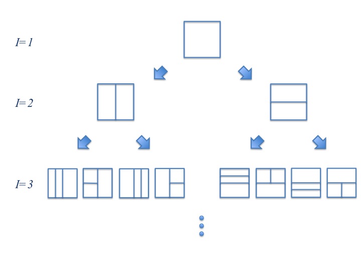
Figure 1: Binary partitions

Now, we define

$$\Theta_{I}=\{f\in\mathcal{F}:f=\sum_{i=1}^{I}\beta_{i}\mathbbm{1}_{\Omega_{i}},\ \mbox{where\ }\sum_{i=1}^{I}\beta_{i}\mu(\Omega_{i})=1,$$

$$\mbox{and\ }\{\Omega_{i}\}_{i=1}^{I}\mbox{ is\ a\ binary\ partition\ of\ $\Omega$\ of\ size\ $I$.}\}$$

This is to say, $\Theta_{I}$ is the collection of piecewise constant density functions supported by the binary partitions of size $I$. Then these $\Theta_{I}$ constitute a sequence of approximating spaces to $\mathcal{F}$ (i.e. a sieve, see [10] and [26] for background on sieve theory).

We take the metric on $\mathcal{F}$ and $\Theta_{I}$ to be Hellinger distance, which is defined by

$$\rho(f,g)=\left(\int_{\Omega}\left(\sqrt{f(y)}-\sqrt{g(y)}\right)^{2}dy\right)^{1/2},\ f,g\in\mathcal{F}.$$ (2.1)

For $f,g\in\Theta_{I}$, let $f=\sum_{i=1}^{I}\beta_{i}^{1}\mathbbm{1}_{\Omega_{i}^{1}}$ and $g=\sum_{i=1}^{I}\beta_{i}^{2}\mathbbm{1}_{\Omega_{i}^{2}}$, where $\{\Omega_{i}^{1}\}_{i=1}^{I}$ and $\{\Omega_{i}^{2}\}_{i=1}^{I}$ are binary partitions of $\Omega$. Then the Hellinger distance between $f$ and $g$ can be written more explicitly as

$$\rho^{2}(f,g)=\sum_{i=1}^{I}\sum_{j=1}^{I}\left(\sqrt{\beta_{i}^{1}}-\sqrt{\beta_{j}^{2}}\right)^{2}\mu\left(\Omega_{i}^{1}\cap\Omega_{j}^{2}\right).$$ (2.2)

We also introduce the Kullback-Leibler divergence, which is defined to be

$$K(f,g)=\mathbb{E}_{f}\left(\log\frac{f(Y)}{g(Y)}\right).$$

Note the Kullback-Leibler divergence is a stronger distance compared to the Hellinger distance, in the sense that for any $f,g\in\mathcal{F}$, $\rho^{2}(f,g)\leq K(f,g)$.

We further restrict our interest to a subsect $\mathcal{F}_{0}\subset\mathcal{F}$ of densities which satisfy the following two conditions: First, $\int_{\Omega}f^{2}<\infty$. Second, for any $f\in\mathcal{F}_{0}$, there exists a sequence of approximations $f_{I}\in\Theta_{I}$ such that $\rho(f,f_{I})\leq AI^{-r}$, where $r$ is a parameter characterizing the decay rate of the approximation error, $A$ is a constant that may depend on $f$. In order to demonstrate that $\mathcal{F}_{0}$ is still a rich class, from Section 4 to Section 6, we study several specific density classes belonging to $\mathcal{F}_{0}$, which are frequently occurred in statistical modelding.

2.2 The sieve MLE

For any $f\in\Theta_{I}$, the log-likelihood is defined to be

$$L_{n}(f)=\sum_{j=1}^{n}\log f(Y_{j})=\sum_{i=1}^{I}N_{i}\log\beta_{i},$$ (2.3)

where $N_{i}$ is the count of data points in $\Omega_{i}$, i.e., $N_{i}=\mbox{card}\{j:Y_{j}\in\Omega_{i},1\leq j\leq n\}$. The maximum likelihood estimator on $\Theta_{I}$ is defined to be

$$\hat{f}_{n,I}=\arg\max_{f\in\Theta_{I}}L_{n}(f).$$ (2.4)

We claim that $\hat{f}_{n,I}$ is well defined. This is true because given the binary partition $\{\Omega_{i}\}_{i=1}^{I}$, the underlying distribution becomes a multinomial one, and $(\beta_{1},\cdots,\beta_{I})$ can be determined by maximizing the log-likelihood. And within each $\Theta_{I}$, the number of possible binary partitions is finite. Since $\Theta_{I}$ constitute a sieve to $\mathcal{F}_{0}$, this sequence of estimators is also called the sieve maximum likelihood estimator (sieve MLE).

In order to illustrating how the idea of partition learning is incorporated in this framework, given the binary partition $\mathcal{A}=\{\Omega_{i}\}_{i=1}^{I}$, we can derive the maximum of the likelihood values achieved by histograms on that partition, which has a closed-form expression

$$L_{n}(\mathcal{A})=\sum_{i=1}^{I}N_{i}\log\left(\frac{N_{i}}{n\mu(\Omega_{i})}\right).$$

We treat this as a score of the partition $\mathcal{A}$. By maximizing the score over all the binary partitions of a fixed size, we learn a most promising one which adapts to the true density function. Then $\hat{f}_{n,I}$ is simply the histogram based on that partition.

2.3 Main results on convergence rate

Having defined a sequence of maximum likelihood estimators $\hat{f}_{n,I}$, we are now ready to state the main results on the rate at which $\hat{f}_{n,I}$ converges to $f_{0}$.

Theorem 2.1.

For any $f_{0}\in\mathcal{F}_{0}$, $\hat{f}_{n,I}$ is the maximum likelihood estimator over $\Theta_{I}$. $A$ and $r$ are the parameters that characterize achievable approximation errors to $f_{0}$ by the elements in $\Theta_{I}$. Assume that $n$ and $I$ satisfy

$$I=\left((2^{8}A^{2}r/c_{1})\frac{n}{\log n}\right)^{\frac{1}{2r+1}},$$ (2.5)

where the constant $c_{1}$ can be chosen to be in $(0,1)$. Then the convergence rate of the sieve MLE is $n^{-\frac{r}{2r+1}}(\log n)^{(\frac{1}{2}+\frac{r}{2r+1})}$, in the sense that

$$\mathbb{P}_{f_{0}}\left(\rho(\hat{f}_{n,I},f_{0})\geq Dn^{-\frac{r}{2r+1}}(\log n)^{(\frac{1}{2}+\frac{r}{2r+1})}\right)\rightarrow 0,$$

where $D$ is a constant.

Remark 2.1.

It is possible to partition the sample space in a more flexible way. In particular, the analysis and resulting rate remain the same if we replace binary partition at the mid-point by binary partition at a point chosen from a fixed sized grid (e.g. regular equi-spaced grid).

From this theorem, we see that the convergence rate does not directly depend on the dimension of the problem. Instead, it only depends on how well the true density can be approximated by the sieve. As $r$ increases, up to a $\log n$ term, the rate gets close to the parametric rate of $n^{-1/2}$.

The analysis in this paper will demonstrate that the optimal convergence rate can be achieved by balancing the sample size with the complexity of the approximating spaces. On one hand, the complexity of $\Theta_{I}$ affects the convergence rate in a way that, the richer the approximating spaces the lower bias the estimators have. Conversely, given a sample $Y_{1},Y_{2},\cdots,Y_{n}$ of fixed size, there is a point beyond which the limited amount of information conveyed in the data may be overwhelmed by the overly-complex approximating spaces. A major contribution of the main result is that it clarifies how to strike the balance between the sample size and the complexity of the approximating spaces.

3 Proof of Theorem 2.1

This section is devoted to the proof of the main theorem. Studies of convergence rate invariably rely on the previous results from studies of empirical process indexed by log-likelihood ratios. However, while the results in the classical work by Wong and Shen ([26] and [31]) are the most applicable ones to our study, they must be modified to adapt to the current settings. The following is an outline of the proof.

In Section 3.1 we briefly discuss metric entropy with bracketing, which measures the complexity of the approximating spaces by “counting” how many pairs of functions in an $\epsilon$-net are needed to provide simultaneous upper and lower bounds of all the elements. An important result of this section is an upper bound for the bracketing metric entropy of $\Theta_{I}$. In Section 3.2, a large-deviation type inequality for the likelihood ratio surface follows.

Previous results on the convergence rate of sieve MLE assume that the true parameter can be approximated by the sieve under Kullback-Leibler divergence. Here, we switch to the weaker Hellinger distance, because under the current settings, we can obtain an explicit bound for the Kullback-Leibler divergence in terms of the Hellinger distance. Thus our results are more general than those in [31] for this type of density estimation problems.

Finally in Section 3.4, we establish the main result of the convergence rate. After splitting the tail probability into two parts corresponding to variance and bias, we apply the results obtained in Section 3.2 and 3.3 to bound each of them respectively.

3.1 Calculation of the metric entropy with bracketing

A general discussion of metric entropy can be found in [14]. In this section, we introduce a form of metric entropy with bracketing corresponding to current parameter space, and provide an upper bound for the bracketing metric entropy of the approximating spaces defined in Section 2.1.

Definition 3.1.

Let $(\Theta,\rho)$ be a seperable pseudo-metric space. $\Theta(\epsilon)$ is a finite set of pairs of functions $\{(f_{j}^{L},f_{j}^{U}),j=1,\cdots,N\}$ satisfying

$$\rho(f_{j}^{L},f_{j}^{U})\leq\epsilon\ for\ j=1,\cdots,N,$$ (3.1)

and for any $f\in\Theta$, there is a $j$ such that

$$f_{j}^{L}\leq f\leq f_{j}^{U}.$$ (3.2)

Let

$$N(\epsilon,\Theta,\rho)=min\{card\ \Theta(\epsilon):(\ref{eq:entropyDefC1})\ and\ (\ref{eq:entropyDefC2})\ are\ satisfied\}.$$ (3.3)

Then, we define the metric entropy with bracketing of $\Theta$ to be

$$H(\epsilon,\Theta,\rho)=\log N(\epsilon,\Theta,\rho).$$ (3.4)

Recall that $\Theta_{1},\cdots,\Theta_{I},\cdots$ are the approximating spaces defined in section 2.1. The next two lemmas are devoted to an upper bound for the bracketing metric entropy of $\Theta_{I}$.

Lemma 3.1.

Take $\rho$ to be the Hellinger distance. Let $\Theta_{I}^{\mathcal{A},d}=\{f\in\Theta_{I}:\ f\ is\ supported\ by\ the\ binary\ partition\ \mathcal{A}=\{\Omega_{i}\}_{i=1}^{I},\ and\ \rho(f,f_{0})\leq d\}$. Then,

$$H(u,\Theta_{I}^{\mathcal{A},d},\rho)\leq\frac{I}{2}\log I+I\log\frac{d}{u}+b^{\prime},$$ (3.5)

where $b^{\prime}$ is a constant not dependent on the binary partition.

Proof.

Assume $f=\sum_{i=1}^{I}\beta_{i}\mathbbm{1}_{\Omega_{i}}$. When the binary partitions $\{\Omega_{i}\}_{i=1}^{I}$ are fixed, there exits a one-to-one correspondance between any $f\in\Theta_{I}^{\mathcal{A},d}$ and an $I$-dimensional vector $(\sqrt{\beta_{1}\mu(\Omega_{1})},\cdots,\sqrt{\beta_{I}\mu(\Omega_{I})})$. As a consequence of Cauchy-Schwartz inequality,

$$\rho(f,f_{0})^{2} = \sum_{i=1}^{I}\int_{\Omega_{i}}(\sqrt{\beta_{i}}-\sqrt{f_{0}(x)})^{2}\mu(dx)$$

$$\geq \sum_{i=1}^{I}\mu(\Omega_{i})(\int_{\Omega_{i}}(\sqrt{\beta_{i}}-\sqrt{f_{0}(x)})\frac{\mu(dx)}{\mu(\Omega_{i})})^{2}$$

$$= \sum_{i=1}^{I}\mu(\Omega_{i})(\sqrt{\beta_{i}}-\frac{\int_{\Omega_{i}}\sqrt{f_{0}(x)}\mu(dx)}{\mu(\Omega_{i})})^{2}.$$

Then, we have,

$$\{(\sqrt{\beta_{1}\mu(\Omega_{1})},\cdots,\sqrt{\beta_{I}\mu(\Omega_{I})}):\sum_{i=1}^{I}\int_{\Omega_{i}}(\sqrt{\beta_{i}}-\sqrt{f_{0}(x)})^{2}\mu(dx)\leq d^{2}\}$$

$$\subset \{(\sqrt{\beta_{1}\mu(\Omega_{1})},\cdots,\sqrt{\beta_{I}\mu(\Omega_{I})}):\sum_{i=1}^{I}(\sqrt{\beta_{i}\mu(\Omega_{i})}-\frac{\int_{\Omega_{i}}\sqrt{f_{0}(x)}\mu(dx)}{\sqrt{\mu(\Omega_{i})}})^{2}\leq d^{2}\}$$

$$=: B_{I}^{\mathcal{A},d}.$$

If we treat the element in $\Theta_{I}^{\mathcal{A},d}$ as the $I$-dimensional vector $(\sqrt{\beta_{1}\mu(\Omega_{1})},\cdots,\sqrt{\beta_{I}\mu(\Omega_{I})})$, then from the above inclusion relation we learn that, $\Theta_{I}^{\mathcal{A},d}\subset B_{I}^{\mathcal{A},d}$. We also note that the Hellinger distance on $B_{I}^{\mathcal{A},d}$ is equivalent to the $L_{2}$ norm on the $I$-dimensional Euclidean space. Thus,

$$N(u,\Theta_{I}^{\mathcal{A},d},\rho)\leq N(u,B_{I}^{\mathcal{A},d},\|\cdot\|_{2}).$$ (3.6)

Because the metric entropy is invariant under translation, calculating the bracketing metric entropy of $B_{I}^{\mathcal{A},d}$ is equivalent to calculating that of

$$\tilde{B}_{I}^{\mathcal{A},d}:=\{\left(\sqrt{\beta_{1}\mu(\Omega_{1})},\cdots,\sqrt{\beta_{I}\mu(\Omega_{I})}\right):\sum_{i=1}^{I}\left(\sqrt{\beta_{i}\mu(\Omega_{i})}\right)^{2}\leq d^{2}\}.$$

The unit sphere under $L_{2}$-norm is

$$S=\{\left(\sqrt{\beta_{1}\mu(\Omega_{1})},\cdots,\sqrt{\beta_{I}\mu(\Omega_{I})}\right):\sum_{i=1}^{I}\left(\beta_{i}\mu(\Omega_{i})\right)\leq 1\}.$$

The unit sphere under $L_{\infty}$-norm is

$$S_{\infty}=\{\left(\sqrt{\beta_{1}\mu(\Omega_{1})},\cdots,\sqrt{\beta_{I}\mu(\Omega_{I})}\right):\max_{1\leq i\leq I}\sqrt{\beta_{i}\mu(\Omega_{i})}\leq 1\}.$$

Note that $\max_{1\leq i\leq I}\sqrt{\beta_{i}\mu(\Omega_{i})}\leq 1/\sqrt{I}$ implies that $\sum_{i=1}^{I}\beta_{i}\mu(\Omega_{i})\leq 1$, and $\sum_{i=1}^{I}\beta_{i}\mu(\Omega_{i})\leq d^{2}$ implies that $\max_{1\leq i\leq I}\sqrt{\beta_{i}\mu(\Omega_{i})}\leq d$, we have

$$S\subset\tilde{B}_{I}^{\mathcal{A},d}\subset dS_{\infty}\mbox{\ and\ }S_{\infty}\subset\sqrt{I}S.$$ (3.7)

Therefore,

$$N(u,\Theta_{I}^{\mathcal{A},d},\rho) \leq N(u,\tilde{B}_{I}^{\mathcal{A},d},\|\cdot\|_{2})$$

$$\leq \left(\frac{d\sqrt{I}}{u}+2\right)^{I}$$

$$\leq b^{\prime}I^{I/2}(d/u)^{I},$$

where $b^{\prime}$ is a constant not dependent on the partiton. The desired result follows. ∎

Lemma 3.2.

Under the same assumptions as in Lemma 3.1, let $\Theta_{I}^{d}=\{f\in\Theta_{I}:\rho(f,f_{0})\leq d\}$. Then,

$$H(u,\Theta_{I}^{d},\rho)$$ (3.8)

$$\leq I\log p+(I+1)\log(I+1)+\frac{I}{2}\log I+I\log\frac{d}{u}+b,$$

where $b$ is a constant not dependent on $I$ or $d$.

Proof.

According to the construction of the sieve, given the size $I$, the number of possible binary partitions is upper bounded by $p^{I}I!$ ($p$ is the dimension of the Euclidean space). Therefore,

$$N(u,\Theta_{I}^{d},\rho) \leq p^{I}I!N(u,\Theta_{I}^{\mathcal{A},d},\rho)$$

$$\leq b^{\prime}p^{I}I!I^{I/2}(d/u)^{I},$$

and,

$$\ H(u,\Theta_{I}^{d},\rho)$$ (3.9)

$$\leq I\log p+(I+1)\log(I+1)+\frac{I}{2}\log I+I\log\frac{d}{u}+b.$$

∎

3.2 An inequality for the likelihood ratio surface

In this section, we focus on bounding the tail behavior of the likelihood ratio. First, we cite a theorem in [31], which gives a uniform exponential bound for likelihood ratios.

Theorem 3.1 (Wong and Shen (1995)).

Let $\rho$ be the Hellinger distance and $\mathcal{P}_{n}$ be a space of densities. There exist positive constants $a>0$, $c$, $c_{1}$ and $c_{2}$, such that, for any $\epsilon>0$, if

$$\int_{\epsilon^{2}/2^{8}}^{\sqrt{2}\epsilon}H^{1/2}(u/a,\mathcal{P}_{n},\rho)du\leq cn^{1/2}\epsilon^{2},$$ (3.10)

then

$$\mathbb{P}_{f_{0}}\Big{(}\sup_{\{\rho(f,f_{0})\geq\epsilon,f\in\mathcal{P}_{n}\}}\prod_{i=1}^{n}\frac{f(Y_{i})}{f_{0}(Y_{i})}\geq\exp(-c_{1}n\epsilon^{2})\Big{)}\leq 4\exp(-c_{2}n\epsilon^{2}),$$

where $\mathbb{P}_{f_{0}}$ is understood to be the outer probability mesure under $f_{0}$. The constants $c_{1}$ and $c_{2}$ can be chosen in $(0,1)$ and $c$ can be set as $(2/3)^{5/2}/512$.

Combining the theorem with the entropy bounds in Section 3.1 gives the desired inequality, which is summarized in the next corollary.

Corollary 3.1.

Let $\delta_{n,I}=(\frac{I\log I}{n/\log n})^{1/2}$. When $n$ and $I$ are sufficiently large, we have

$$\mathbb{P}_{f_{0}}\Big{(}\sup_{\{\rho(f,f_{0})\geq\delta_{n,I},f\in\Theta_{I}\}}\prod_{i=1}^{n}\frac{f(Y_{i})}{f_{0}(Y_{i})}\geq\exp(-c_{1}n\delta_{n,I}^{2})\Big{)}\leq 4\exp(-c_{2}n\delta_{n,I}^{2}).$$

Proof.

The key to the proof is to check condition (3.10) so that we can apply Theorem 3.1 to the sequence of approximating spaces $\Theta_{I}$. By Lemma 3.2,

$$\int_{\delta_{n,I}^{2}/2^{8}}^{\sqrt{2}\delta_{n,I}}H^{1/2}(u/a,\Theta_{I},\rho)du$$ (3.11)

$$\leq \int_{\delta_{n,I}^{2}/2^{8}}^{\sqrt{2}\delta_{n,I}}\left(I\log(4pa)+2(I+1)\log(I+1)-I\log u\right)^{1/2}du$$

$$\sim I^{1/2}\int_{\delta_{n,I}^{2}/2^{8}}^{\sqrt{2}\delta_{n,I}}\left(\log\frac{I^{2}}{u}\right)^{1/2}du.$$

We calculate the integral and obtain

$$\eqref{eq:entropybound}$$

$$\leq I^{1/2}\left(u\sqrt{\log\frac{I^{2}}{u}}-\frac{\sqrt{\pi}}{2}I^{2}\mbox{erf}\left(\sqrt{\log\frac{I^{2}}{u}}\right)\right)|_{\delta_{n,I}^{2}/2^{8}}^{\sqrt{2}\delta_{n,I}}$$

$$\leq I^{1/2}(\sqrt{2}\delta_{n,I}\sqrt{\log\frac{I^{2}}{\sqrt{2}\delta_{n,I}}}-\frac{\sqrt{\pi}}{2}I^{2}\mbox{erf}\left(\sqrt{\log\frac{I^{2}}{\sqrt{2}\delta_{n,I}}}\right)-\frac{\delta_{n,I}^{2}}{2^{8}}\sqrt{\log\frac{2^{8}I^{2}}{\delta_{n,I}^{2}}}$$

$$+\frac{\sqrt{\pi}}{2}I^{2}\mbox{erf}\left(\sqrt{\log\frac{2^{8}I^{2}}{\delta_{n,I}^{2}}}\right))$$

$$\sim I^{1/2}\left(\delta_{n,I}\sqrt{\log\frac{I^{2}}{\delta_{n,I}}}+\frac{\sqrt{\pi}}{2}I^{2}\left(\mbox{erf}(\sqrt{\log\frac{2^{8}I^{2}}{\delta_{n,I}^{2}}})-\mbox{erf}(\sqrt{\log\frac{I^{2}}{\sqrt{2}\delta_{n,I}}})\right)\right)$$

$$\sim I^{1/2}\left(\delta_{n,I}\sqrt{\log\frac{I^{2}}{\delta_{n,I}}}+\frac{\sqrt{\pi}}{2}I^{2}\left(1-\frac{\frac{\delta_{n,I}^{2}}{2^{8}I^{2}}}{\sqrt{\pi\log\frac{2^{8}I^{2}}{\delta_{n,I}^{2}}}}-1+\frac{\frac{\sqrt{2}\delta_{n,I}}{I^{2}}}{\sqrt{\pi\log\frac{I^{2}}{\sqrt{2}\delta_{n,I}}}}\right)\right)$$

$$\sim I^{1/2}\delta_{n,I}\sqrt{\log\frac{I^{2}}{\delta_{n,I}}}$$

$$\leq c\sqrt{n}\delta_{n,I}^{2}.$$

Therefore, condition (3.10) is satisfied. The desired result follows from Theorem 3.1. ∎

3.3 An inequality for the Kullback-Leibler divergence

It is well known that Hellinger distance can be bounded by Kullback-Leibler divergence. In [31], the authors showed that the other direction also holds under mild conditions. This type of result becomes quite useful in this paper because it would allow us to study the convergence rate under the weaker Hellinger distance. We first cite the result from their paper. It enables us to obtain a more explicite bound for density functions in $\mathcal{F}_{0}$ in the later part of this section.

Lemma 3.3 (Wong and Shen (1995) Theorem 5).

Let $f$, $f_{0}$ be two densities, $\rho^{2}(f_{0},f)\leq\epsilon^{2}$. Suppose that $M_{\lambda}^{2}=\int_{\{f_{0}/f\geq e^{1/\lambda}\}}f_{0}(f_{0}/f)^{\lambda}<\infty$ for some $\lambda\in(0,1]$. Then for all $\epsilon^{2}\leq\frac{1}{2}(1-e^{-1})^{2}$, we have

$$\int f_{0}\log(\frac{f_{0}}{f})\leq\big{[}6+\frac{2\log 2}{(1-e^{-1})^{2}}+\frac{8}{\lambda}\max\big{(}1,\log(\frac{M_{\lambda}}{\epsilon})\big{)}\big{]}\epsilon^{2},$$

$$\int f_{0}\big{(}\log(\frac{f_{0}}{f})\big{)}^{2}\leq 5\epsilon^{2}\big{[}\frac{1}{\lambda}\max\big{(}1,\log(\frac{M_{\lambda}}{\epsilon})\big{)}\big{]}^{2}.$$

When $f_{0}$ is the true density function and $f$ is an approximation to $f_{0}$ in $\Theta_{I}$, we can obtain a more explicit bound of the Kullback-Leibler divergence. The result is summarized in the lemma below.

Lemma 3.4.

$f_{0}$ is a density function on $\Omega$. If $f_{0}\in\mathcal{F}_{0}$, then we can find $g\in\Theta_{I}$, such that

$$\int f_{0}\log(f_{0}/g)\leq 128A^{2}rI^{-2r}\log I,$$

$$\int f_{0}(\log(f_{0}/g))^{2}\leq 320A^{2}r^{2}I^{-2r}(\log I)^{2}.$$

Proof.

Assume that $f=\sum_{i=1}^{I}\beta_{i}\mathbbm{1}_{\Omega_{i}}$, where $\{\Omega_{i}\}_{i=1}^{I}$ is a binary partition of $\Omega$. From the property of $L_{2}$-projection, we have

$$\rho^{2}(f_{0},f) = \sum_{i=1}^{I}\int_{\Omega_{i}}(\sqrt{f_{0}(x)}-\sqrt{\beta_{i}})^{2}\mu(dx)$$

$$\geq \sum_{i=1}^{I}\int_{\Omega_{i}}\left(\sqrt{f_{0}}-\frac{\int_{\Omega_{i}}\sqrt{f_{0}}}{\mu(\Omega_{i})}\right)^{2}.$$

Let $h=\sum_{i=1}^{I}\left(\frac{\int_{\Omega_{i}}\sqrt{f_{0}}}{\mu(\Omega_{i})}\right)^{2}\mathbbm{1}_{\Omega_{i}}$, then

$$\int_{\Omega}h=\sum_{i=1}^{I}\frac{(\int_{\Omega_{i}}\sqrt{f_{0}})^{2}}{\mu(\Omega_{i})}\leq\sum_{i=1}^{I}\frac{(\int_{\Omega_{i}}f_{0})\mu(\Omega_{i})}{\mu(\Omega_{i})}=1.$$

Let $g=\frac{h}{\int_{\Omega}h}$, then $g$ is a density function, and

$$\rho^{2}(f_{0},g) = \|\sqrt{f_{0}}-\sqrt{h}+\sqrt{h}-\frac{\sqrt{h}}{\|\sqrt{h}\|_{2}}\|_{2}^{2}$$

$$\leq 2\|\sqrt{f_{0}}-\sqrt{h}\|_{2}^{2}+2(1-\frac{1}{\|\sqrt{h}\|_{2}})^{2}\|\sqrt{h}\|_{2}^{2}$$

$$\leq 2\rho^{2}(f_{0},f)+2(1-\|\sqrt{h}\|_{2}^{2})$$

$$= 2\rho^{2}(f_{0},f)+2\|\sqrt{f_{0}}-\sqrt{h}\|_{2}^{2}$$

$$\leq 4\rho^{2}(f_{0},f).$$

For density functions $f_{0}$ and $g$,

$$M_{1/4}^{2} = \sum_{i=1}^{I}\int_{\Omega_{i}\cap\{f_{0}/g>e^{4}\}}f_{0}\left(\frac{f_{0}}{\left(\frac{\int_{\Omega_{i}}\sqrt{f_{0}}}{\|\sqrt{h}\|_{2}\mu(\Omega_{i})}\right)^{2}}\right)^{1/4}$$

$$\leq \sum_{i=1}^{I}\frac{\int_{\Omega_{i}}f_{0}^{1+1/4}}{\left(\frac{\int_{\Omega_{i}}\sqrt{f_{0}}}{\mu(\Omega_{i})}\right)^{1/2}}$$

$$\leq \sum_{i=1}^{I}\frac{(\int_{\Omega_{i}}f_{0}^{1/2})^{1/2}(\int_{\Omega_{i}}f_{0}^{2})^{1/2}}{\left(\frac{\int_{\Omega_{i}}\sqrt{f_{0}}}{\mu(\Omega_{i})}\right)^{1/2}}=\sum_{i=1}^{I}(\int_{\Omega_{i}}f_{0}^{2})^{1/2}(\mu(\Omega_{i}))^{1/2}$$

$$\leq \left(\int_{\Omega}f_{0}^{2}\right)^{1/2}.$$

Therefore, if we set $\lambda=1/4$, when $I$ is large enough

$$\int f_{0}\log(f_{0}/g) \leq [6+\frac{2\log 2}{(1-e^{-1})^{2}}+32\max(1,\log\frac{(\int f_{0}^{2})^{1/4}}{2AI^{-r}})]\cdot 4A^{2}I^{-2r}$$

$$\leq 128A^{2}rI^{-2r}\log I.$$

Similarly,

$$\int f_{0}(\log(f_{0}/g))^{2}\leq 320A^{2}r^{2}I^{-2r}(\log I)^{2}.$$

∎

3.4 Convergence rate

In this section, we apply the above large-deviation type inequality and the bound of the Kullback-Leibler divergence to derive convergence rate of the sieve MLE for $f_{0}\in\mathcal{F}_{0}$.

proof of Theorem 2.1.

For any $g\in\Theta_{I}$ and $D>1$, we have

$$\mathbb{P}\left(\rho(f_{0},\hat{f}_{n,I})\geq D\delta_{n,I}\right)\leq\mathbb{P}_{f_{0}}\left(\sup_{\{\rho(f_{0},f)\geq D\delta_{n,I},f\in\Theta_{I}\}}\prod_{j=1}^{n}f(Y_{j})/g(Y_{j})\geq 1\right),$$

where $\mathbb{P}_{f_{0}}$ is understood to be the outer probability measure under $f_{0}$.

Let $C=\{f\in\Theta_{I}:\rho(f_{0},f)\geq D\delta_{n,I}\}$. Then for $g\in\Theta_{I}$,

$$\mathbb{P}_{f_{0}}\left(\sup_{f\in C}\prod_{j=1}^{n}\frac{f(Y_{j})}{g(Y_{j})}\geq 1\right)\leq P_{1}+P_{2},$$

where

$$P_{1}=\mathbb{P}_{f_{0}}\left(\sup_{f\in C}\prod_{j=1}^{n}\frac{f(Y_{j})}{f_{0}(Y_{j})}\geq\exp\left(-c_{1}n(D\delta_{n,I})^{2}\right)\right),$$

$$P_{2}=\mathbb{P}\left(\prod_{j=1}^{n}\frac{f_{0}(Y_{j})}{g(Y_{j})}\geq\exp\left(c_{1}n(D\delta_{n,I})^{2}\right)\right).$$

In regards of $P_{1}$, Corollary 3.1 still applies here if we replace $\delta_{n,I}$ by $D\delta_{n,I}$. Thus, $P_{1}\leq 4\exp(-c_{2}nD^{2}\delta^{2}_{n,I})$.

To bound $P_{2}$, we write

$$P_{2} = \mathbb{P}\left(\sum_{j=1}^{n}\log\left(\frac{f_{0}}{g}\right)(Y_{j})\geq c_{1}n(D\delta_{n,I})^{2}\right)$$

$$= \mathbb{P}\left(\sum_{j=1}^{n}\left[\log\left(\frac{f_{0}}{g}\right)(Y_{j})-\mathbb{E}\log\left(\frac{f_{0}}{g}\right)\right]\geq c_{1}n(D\delta_{n,I})^{2}-n\int f_{0}\log\left(\frac{f_{0}}{g}\right)\right).$$

If $\int f_{0}\log(f_{0}/g)<c_{1}D^{2}\delta^{2}_{n,I}$, then

$$P_{2}\leq\frac{n\int f_{0}\log\left(\frac{f_{0}}{g}\right)^{2}}{n^{2}\left(c_{1}D^{2}\delta^{2}_{n,I}-\int f_{0}\log\left(\frac{f_{0}}{g}\right)\right)^{2}}.$$

Based on our assumption, there exists $f_{I}\in\Theta_{I}$, such that $\rho(f_{0},f_{I})\leq AI^{-r}$. Then from Lemma 3.4, we know that

$$\int f_{0}\log(f_{0}/f_{I})\leq 128A^{2}rI^{-2r}\log I,$$

$$\int f_{0}(\log(f_{0}/f_{I}))^{2}\leq 320A^{2}r^{2}I^{-2r}(\log I)^{2}.$$

Therefore,

$$\inf_{g\in\Theta_{I}}P_{2}\leq\frac{320A^{2}r^{2}I^{-2r}(\log I)^{2}}{n\left(c_{1}D^{2}\delta^{2}_{n,I}-128A^{2}rI^{-2r}\log I\right)^{2}}.$$

If we take $I=\left((2^{8}A^{2}r/c_{1})\frac{n}{\log n}\right)^{\frac{1}{2r+1}}$, then the condition $\int f_{0}\log(f_{0}/f_{I})<c_{1}D^{2}\delta^{2}_{n,I}$ is satisfied. If $n$ and $I$ are matched in this way, the order of $\delta_{n,I}$ determines the final convergence rate, which is $n^{-\frac{r}{2r+1}}(\log n)^{(\frac{1}{2}+\frac{r}{2r+1})}$. This finishes the proof. ∎

4 Application to spatial adaptation

In this section, we assume that the density concentrates spatially. Mathematically, this implies the density function satisfies a type of spatial sparsity. In the past two decades, sparsity has become one of the most discussed types of structure under which we are able to overcome the curse of dimensionality. A remarkable example is that it allows us to solve high-dimensional linear models, especially when the system is underdetermined. It would be interesting to study how we could benefit from the sparse structure when performing density estimation. This section is devoted to this purpose. Under current settings, it is natural to characterize the spatial sparsity by controlling the decay rate of the ordered Haar wavelet coefficients. After introducing the high-dimensional Haar basis in Section 4.1, we provide a rigorous characterization of the sparsity condition in Section 4.2, and illustrate this characterization by several examples. In Section 4.3, we demonstrate that the sparse structure allows fast convergence by calculating the explicit convergence rate.

4.1 High-dimensional Haar basis

Haar basis is the simplest but widely used wavelet basis. In one dimension, the Haar wavelet’s mother wavelet function is

$$\psi(y)=\begin{cases}1&\mbox{if }0\leq y<1/2,\\ -1&\mbox{if }1/2\leq y<1,\\ 0&\mbox{otherwise.}\end{cases}$$

And its scaling function is

$$\phi(y)=\begin{cases}1&\mbox{if }0\leq y<1,\\ 0&\mbox{otherwise.}\end{cases}$$

Here, we take the two-dimensional case to illustrate how the system is built. This construction can be extended to high dimensional cases as well.

The two-dimensional scaling function is defined to be

$$\phi\phi(y^{1},y^{2}):=\phi(y^{1})\phi(y^{2}),$$

and three wavelet functions are

$$\phi\psi(y^{1},y^{2}):=\phi(y^{1})\psi(y^{2}),$$

$$\psi\phi(y^{1},y^{2}):=\psi(y^{1})\phi(y^{2}),$$

$$\psi\psi(y^{1},y^{2}):=\psi(y^{1})\psi(y^{2}).$$

If we use a superscript $l$ to index the scaling level of the wavelet function and subscripts $i$ and $j$ ($i$ and $j$ can be 0 or 1) to denote the horizontal and vertical translations respectively, then the scales and translates of the three wavelet functions $\phi\psi$, $\psi\phi$ and $\psi\psi$ are defined to be

$$\phi\psi_{ij}^{l}(y^{1},y^{2}):=(\sqrt{2})^{2\cdot l}\phi\psi(2^{l}y^{1}-i,2^{l}y^{2}-j),$$

$$\psi\phi_{ij}^{l}(y^{1},y^{2}):=(\sqrt{2})^{2\cdot l}\psi\phi(2^{l}y^{1}-i,2^{l}y^{2}-j),$$

$$\psi\psi_{ij}^{l}(y^{1},y^{2}):=(\sqrt{2})^{2\cdot l}\psi\psi(2^{l}y^{1}-i,2^{l}y^{2}-j).$$

These functions together with the single scaling function $\phi\phi$ define the two-dimensional Haar wavelet basis $\Psi$.

4.2 Spatial sparsity

Let $f$ be a $p$ dimensional density function and $\Psi$ the $p$-dimensional Haar basis constructed as above. We will work with $g=\sqrt{f}$ first. Note that $g\in L^{2}([0,1]^{p})$. Thus we can expand $g$ with respect to $\Psi$ as $g=\sum_{\psi\in\Psi}<g,\psi>\psi$ (here $\psi$ is a basis function instead of the Haar wavelet’s mother wavelet function defined above). We rearrange this summation by the size of wavelet coefficients. In other words, we order the coefficients as the following

$$|<g,\psi_{(1)}>|\geq|<g,\psi_{(2)}>|\geq\cdots\geq|<g,\psi_{(k)}>|\geq\cdots,$$

then the sparsity condition imposed on the density functions is that the decay of the wavelet coefficients follows a power law,

$$|<g,\psi_{(k)}>|\leq Ck^{-\beta}\mbox{ for all $k\in\mathbb{N}$ and $\beta>1/2$, }$$ (4.1)

where $C$ is a constant.

This condition has been widely used to characterize the sparsity of signals and images ([1] and [3]). In particular, in [5], it was shown that for two-dimensional cases, when $\beta>1/2$, this condition reasonably captures the sparsity of real world images.

Next we use several examples to illustrate how this condition implies the spatial sparsity of the density function.

Example 4.2.1.

Assume that the we are studying a density function in three dimensions. All the mass concentrates in a dyadic cube. Without loss of generality, we assume that $f_{0}=64\mathbbm{1}_{\{0\leq y^{1},y^{2},y^{3}<1/4\}}$, so that all the mass is concentrated in a small cubical subregion. In the three-dimensional case, the single scaling function is $\phi\phi\phi$, and the seven wavelet functions are defined as

$$\chi_{1}=\psi\phi\phi,\ \chi_{2}=\phi\psi\phi,\ \chi_{3}=\phi\phi\psi,$$

$$\chi_{4}=\psi\psi\phi,\ \chi_{5}=\psi\phi\psi,\ \chi_{6}=\phi\psi\psi,$$

$$\chi_{7}=\psi\psi\psi.$$

If we still use the superscript to denote the scaling level and the subscripts to denote the spatial translations, then the expansion of $f_{0}$ with respect to the Haar basis is

$$f_{0}=\phi\phi\phi+\sum_{k=1}^{7}\chi_{k,000}^{(0)}+2\sqrt{2}\sum_{k=1}^{7}\chi_{k,000}^{(1)}.$$

The coefficients display a decaying trend, although the number of them is finite. More generally, any density function whose expansion only has finite terms will satisfy the condition (4.1).

Example 4.2.2.

Assume that the two-dimensional true density function is

$$\begin{pmatrix}Y_{1}\\ Y_{2}\\ \end{pmatrix}\sim\frac{2}{5}\mathcal{N}\left(\begin{pmatrix}0.25\\ 0.25\\ \end{pmatrix},0.05^{2}I_{2\times 2}\right)+\frac{3}{5}\mathcal{N}\left(\begin{pmatrix}0.75\\ 0.75\\ \end{pmatrix},0.05^{2}I_{2\times 2}\right).$$

We perform the Haar transform. The heatmap of the density function is displayed in Figure 2 and the plot of the Haar coefficients is shown in Figure 3. The left panel in Figure 3 is the plot of all the coefficients to level ten from low resolution to high resolution. The middle one is the sorted coefficients according to their absolute value. And the right one is the same as the middle plot but with the abcissa in log-scale. From this we can clearly see that the power-law decay is satisfied, and an empirical estimation of the corresponding $\beta$ can be obtained in this case.

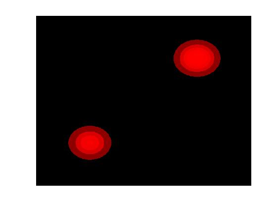
Figure 2: Heatmap of the density

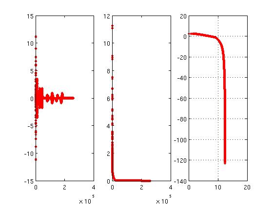
Figure 3: Plots of the 2-dimensional Haar coefficients. The left panel is the plot of all the coefficients from low resolution to high resolution. The middle one is the plot of the sorted coefficients. And the right one is the same as the middle plot but with the abcissa in log scale.

Example 4.2.3.

Let the three-dimensional density function be

$$\begin{pmatrix}Y_{1}\\ Y_{2}\\ Y_{3}\\ \end{pmatrix}\sim\frac{2}{5}\mathcal{N}\left(\begin{pmatrix}0.25\\ 0.25\\ 0.25\\ \end{pmatrix},\begin{pmatrix}0.05^{2}&0.03^{2}&0\\ 0.03^{2}&0.05^{2}&0\\ 0&0&0.05^{2}\\ \end{pmatrix}\right)+\frac{3}{5}\mathcal{N}\left(\begin{pmatrix}0.75\\ 0.75\\ 0.75\\ \end{pmatrix},0.05^{2}I_{3\times 3}\right).$$

In this example, we impose some correlation structure in one component. Haar transform is performed and the behavior of the Haar coefficients is summarized in Figure 4. The arrangement of the plots is the same as that in the previous example. For this three-dimensional example, the power-law decay is still satisfied.

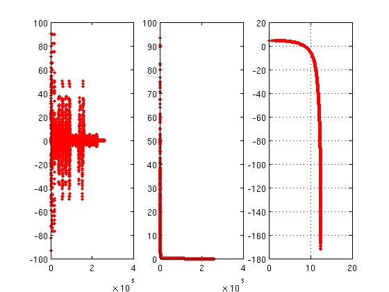
Figure 4: Plots of the 3-dimensional Haar coefficients. The order of the plots is the same as that in Figure 3.

4.3 Convergence rate

Assume that $f_{0}$ is the $p$-dimensional density function satisfy the spatial sparsity condition (4.1). Now we calculate the convergence rate of the sieve MLE.

Lemma 4.1.

Suppose $f_{0}$ is a $p$-dimensional density function. $g_{0}=\sqrt{f_{0}}$ satisfies the condition (4.1). Then there exists a sequence of $f_{I}\in\Theta_{I}$, such that $\rho(f_{0},f_{I})\lesssim I^{-(\beta-1/2)}$, or equivalently, $\rho(f_{0},f_{I})\leq cI^{-(\beta-1/2)}$, where $c$ may depend on $\beta$ and $p$ but not $I$.

Proof.

Let $g_{K}=\sum_{k=1}^{K}<g_{0},\psi_{(k)}>\psi_{(k)}$. From condition (4.1) we have

$$\rho^{2}(f_{0},g_{K}^{2}) = \|g_{0}-g_{K}\|_{2}^{2}=\|\sum_{k=K+1}^{+\infty}<g_{0},\psi_{(k)}>\psi_{(k)}\|_{2}^{2}$$ (4.2)

$$= \sum_{k=K+1}^{+\infty}<g_{0},\psi_{(k)}>^{2}$$

$$\leq C^{2}\sum_{k=K+1}^{+\infty}k^{-2\beta}\leq\frac{C^{2}}{2\beta-1}K^{-(2\beta-1)}.$$

Then we normalize $g_{K}$ to $\tilde{g}_{K}$ and obtain

$$\rho^{2}(f_{0},\tilde{g}_{K}^{2}) = \|g_{0}-\tilde{g}_{K}\|_{2}^{2}$$ (4.3)

$$= \|g_{0}-g_{K}\|_{2}^{2}+(1-\frac{1}{\|g_{K}\|_{2}})^{2}\|g_{K}\|_{2}^{2}$$

$$\leq \|g_{0}-g_{K}\|_{2}^{2}+1-\|g_{K}\|_{2}^{2}$$

$$= 2\|g_{0}-g_{K}\|_{2}^{2}$$

$$\leq \frac{2C^{2}}{2\beta-1}K^{-(2\beta-1)}.$$

Note that given a supporting rectangle, the positive and negative parts of the Haar basis function defined on it can further divide the original rectangle into smaller subregions, and the total number of such subregions is upper bounded by $2^{p}$. Therefore, $2^{p}K$ is the largest possible sized binary partition on which the density function $\tilde{g}_{K}$ is piecewise constant. Replacing $K$ in (4.3) by $I/2^{p}$, we get the desired result of approximation rate. ∎

The next theorem calculates the convergence rate in this case.

Theorem 4.1.

(Application to spatial adaptation) Assume $f_{0}$ is the same as defined in Lemma (4.1). If we apply the maximum likelihood density estimator based on adaptive partitioning here to estimate the true density function, the convergence rate is $n^{-\frac{\beta-1/2}{2\beta}}(\log n)^{\frac{1}{2}+\frac{\beta-1/2}{2\beta}}$.

Proof.

This follows Theorem 2.1 and Lemma 4.1 directly. ∎

From the theorem we see that the convergence rate only depends on how fast the coefficients decay as opposed to the dimension of the sample space. Thus for large $\beta$, the density estimate is able to take advantage of spatial sparsities to achieve fast convergence rate even in high dimensions.

5 Estimation of functions of bounded variation

In image analysis, the denoised image is usually assumed to be a function of bounded variation. Obtaining an approximation is a crucial procedure before any downstream analysis. Currently, nonlinear approximation, such as wavelet compression [5] and wavelet shrinkage or thresholding [7], has been widely used in this field, contributing to problems including image compression and image segmentation. In this section, we treat the denoised image as a density function, and apply this multivariate density estimation method to obtain the approximation. We evaluate the performance of this method by calculating the convergence rate when the density function is of bounded variation (Section 5.2). Actually, its performance is comparable to that of wavelet thresholding. This point becomes clearer in the companion papar [17], where under Bayesian settings we show that minimax convergence rate can be achieved for the space of bounded variation (BV) up to a logarithmic term. To begin with, we briefly introduce the space BV in Section 5.1.

5.1 The space BV

Let $\Omega=[0,1)^{2}$ be a domain in $\mathbb{R}^{2}$. We define the space $BV(\Omega)$ of functions of bounded variation on $\Omega$ as follows.

For a vector $\nu\in\mathbb{R}^{2}$, the difference operator $\Delta_{\nu}$ along the direction $\nu$ is defined by

$$\Delta_{\nu}(f,y):=f(y+\nu)-f(y).$$

For functions $f$ defined on $\Omega$, $\Delta_{\nu}(f,y)$ is defined whenever $y\in\Omega(\nu)$, where $\Omega(\nu):=\{y:[y,y+\nu]\subset\Omega\}$ and $[y,y+\nu]$ is the line segment connecting $y$ and $y+\nu$. Denote by $e_{l},l=1,2$ the two coordinate vectors in $\mathbb{R}^{2}$. We say that a function $f\in L_{1}(\Omega)$ is in $BV(\Omega)$ if and only if

$$V_{\Omega}(f):=\sup_{h>0}h^{-1}\sum_{l=1}^{2}\|\Delta_{he_{l}}(f,\cdot)\|_{L_{1}(\Omega(he_{l}))}=\lim_{h\rightarrow 0}h^{-1}\sum_{l=1}^{2}\|\Delta_{he_{l}}(f,\cdot)\|_{L_{1}(\Omega(he_{l}))}$$

is finite. The quantity $V_{\Omega}(f)$ is the variation of $f$ over $\Omega$.

$p$-dimensional bounded variation function can be defined similarly. In [6], the author demonstrated that, in one dimension wavelet representations of bounded variation balls are optimal. The result of optimality can be extended to two-dimensional cases as well. Given the fact that the density functions defined on binary partitions are essentially equivalent to the Haar bases, it is natural to ask what the convergence rate will be if we apply this multivariate density estimator to $BV(\Omega)$. This result will be presented in the section below.

5.2 Convergence rate

In this section, we still use the Haar basis defined in Section 4.1. Let $\Lambda$ be the set of indices for the wavelet basis. Each element in $\Lambda$ is a pair of scale and location parameters. We will denote by $\Sigma_{N}$ the spaces consisting of $N$-term approximation in the Haar system, in other words,

$$\Sigma_{N}:=\{\sum_{\lambda\in E}c_{\lambda}\psi_{\lambda}:E\subset\Lambda,|E|\leq N\},$$

where $|E|$ denotes the cardinality of the discrete set $E$.

First, we cite a theorem from [4]. It provides a result on the approximation rate to a function of bounded variation by $\Sigma_{N}$.

Lemma 5.1.

If $f\in BV(\Omega)$ has mean value zero on $\Omega$, we have

$$\inf_{g\in\Sigma_{N}}\|f-g\|_{L_{2}(\Omega)}\leq CN^{-1/2}V_{\Omega}(f),$$ (5.1)

with $C=2592(3\sqrt{5}+\sqrt{3})$.

Assume $f_{0}$ is a density function on $\Omega$ of bounded variation. By subtracting the mean, we can always assume that $\sqrt{f_{0}}$ has mean value zero over $\Omega$. For the square root of $f_{0}$, applying the lemma above, we can find an $N$-term approximation $g$ in the Haar system, such that $\|\sqrt{f_{0}}-g\|_{L_{2}(\Omega)}\lesssim N^{-1/2}$. Translating this inequality into the size of partition, we reach the conclusion that for a density function in $BV(\Omega)$, we can find an approximation in $\Theta_{I}$, such that $\rho(f_{0},f_{I})\lesssim I^{-1/2}$. Now we are ready to state the result of the convergence rate.

Theorem 5.1.

Assume that $f_{0}\in BV(\Omega)$. If we apply the multivariate density estimator based on adaptive partitioning here to estimate $f_{0}$, the convergence rate is $n^{-1/4}(\log n)^{3/4}$.

Proof.

The proof follows Theorem 2.1 and the previous approximation result directly. ∎

6 Application to variable selection

For high dimensional data analysis, selecting significant variables greatly contributes to simplifying the model, improving model interpretability, and reducing overfitting. In the context of density estimation, the variable selection problem is formulated as follows. Assume $f_{0}$ is a $p$-dimensional density function and it only depends on $\tilde{p}$ variables, but we do not know in advance which $\tilde{p}$ variables. We apply the multivariate density estimation method here to the $p$-dimensional density. The essential part of our method is to learn a partition of the support of the true density function, and then to estimate the density on each subregion separately. Because the true density lies in a $\tilde{p}$-dimensional subspace, we may surmise that the corresponding convergence rate only depends on the effective dimension. The goal of this section is to carry out exact calculations to reveal that this is indeed the case. Here, we consider a class of density functions satisfying certain type of continuity. We first provide a mathematical description of this density class in Section 6.2. This description still depends on the Haar transform of the true density function. However, an alternative construction of the high-dimensional Haar basis via tensor product is introduced in Section 6.1 because of some technical issue. We provide the result on the explicite convergence rate in Section 6.3.

6.1 Tensor Haar basis

In one dimension, the Haar wavelet’s mother wavelet function $\psi$ and its scaling function $\phi$ are the same as those defined in Section 4.1. For any $l\in\mathbb{N}$ and $0\leq k<2^{l}$, the Haar function is

$$\psi^{l}_{k}(y)=2^{l/2}\psi(2^{l}y-k).$$

Then Haar basis $\Psi$ is the collection of all Haar functions together with the scale function. Namely,

$$\textbf{$\Psi$}=\{\phi\}\cup\{\psi^{l}_{k},l\in\mathbb{N},0\leq k<2^{l}\}.$$

It is an orthonormal basis for Hilbert space $L^{2}([0,1])$.

Turning to high-dimensional settings, we can obtain an orthonormal basis for $L^{2}([0,1]^{p})$ by using the fact that the Hilbert space $L^{2}([0,1]^{p})$ is isomorphic to the tensor product of $p$ one-dimensional spaces. In detail, if $\mathcal{X}_{1},\cdots,\mathcal{X}_{p}$ are $p$ copies of $L^{2}([0,1])$ and $\Psi_{1}$, $\cdots$, $\Psi_{p}$ are Haar bases of these spaces respectively, then $L^{2}([0,1]^{p})$ is isomorphic to $\bigotimes_{i=1}^{p}\mathcal{X}_{i}$. Define tensor Haar basis $\Psi$ by

$$\textbf{$\Psi$}=\{\psi:\psi=\prod_{i=1}^{p}\psi_{i},\psi_{i}\in\textbf{$\Psi_{i}$}\}.$$

From the property of tensor product of Hilbert spaces, we know that $\Psi$ is an orthonormal basis for $L^{2}([0,1]^{p})$.

6.2 Mixed-Hölder continuity

In this section, we assume the density function satisfies the Mixed-Hölder condition. A similar condition first appeared in [28]. The author showed that tensor Haar basis with large support is efficient in representing certain type of functions on $[0,1]^{p}$. More precisely, if the function satisfies the bounded mixed variation condition, then it can be approximated to error $\epsilon>0$ using no more than $\frac{1}{\epsilon}(\log(\frac{1}{\epsilon}))^{p-1}$ terms, and the volume of the supporting rectangle of the each wavelet basis function involved in the approximation is greater than $\epsilon$. However, the result is restrictive in application since the mixed derivative is not rotationally invariant. In [9], the authors extended the previous approximation scheme to matrix. A significant improvement is that, in their paper, the bounded mixed variation condition is replaced by the Mixed-Hölder condition, which is more natural and accessible. For two-dimensional discrete analyses of matrices, they show that the approximation is still efficient for this class of matrices, and the Mixed-Hölder condition is connected to the decay rate of wavelet coefficients. The idea of controlling the decay rate of wavelet coefficients will be further developed here. It leads to the characterization of the density class under consideration.

For any $f\in\mathcal{F}$, $\sqrt{f}\in L^{2}([0,1]^{p})$. Therefore, we can expand $\sqrt{f}$ with respect to the tensor Haar basis. Let $g=\sqrt{f}$. Then

$$g=\sum_{\psi\in\textbf{$\Psi$}}<g,\psi>\psi,\ \mbox{where}<g,\psi>=\int_{\Omega}g(y)\psi(y)dy.$$

For each tensor Haar function $\psi$, let $R(\psi)$ denote its supporting rectangle. The density class under consideration is defined to be

$$\mathcal{F}_{H}=\{f\in\mathcal{F}:|<\sqrt{f},\psi>|\leq C|R(\psi)|^{\alpha+1/2}\mbox{ for all }\psi\in\textbf{$\Psi$}\},$$

where $C$ is a constant which may depend on $f$, $|R(\psi)|$ denotes the volume of the rectangle and $\alpha$ is a positive constant.

Next, we provide several examples to illustrate how this condition relates to the Mixed-Hölder continuity.

Example 6.2.1.

A real-valued function $f$ on $\mathbb{R}$ is Hölder continuous, if there exist nonnegative constants $C$ and $\alpha\in(0,1]$, such that $|f(x)-f(y)|\leq C|x-y|^{\alpha}$, for all $x,y\in\mathbb{R}$. If square root of the true density function $f_{0}$ is Hölder continuous for some constants $C,\alpha$, then for any Haar basis function $\psi$, $|<\sqrt{f_{0}},\psi>|\leq C|R(\psi)|^{\alpha+1/2}$.

Proof.

From Hölder continuity, we know that for any $x,y\in[0,1]$, $|\sqrt{f_{0}(x)}-\sqrt{f_{0}(y)}|\leq C|x-y|^{\alpha}$. For any point $x_{0}\in R$, we have

$$|<\sqrt{f_{0}},\psi>|^{2} = \left(\int_{R}\sqrt{f_{0}(x)}\psi(x)dx\right)^{2}$$

$$= \left(\int_{R}\left(\sqrt{f_{0}(x)}-\sqrt{f_{0}(x^{\prime})}\right)\psi(x)dx\right)^{2}$$

$$\leq \int_{R}\left(\sqrt{f_{0}(x)}-\sqrt{f_{0}(x^{\prime})}\right)^{2}dx\cdot\int_{R}\psi(x)^{2}dx$$

$$\leq C^{2}\int_{R}|x-x_{0}|^{2\alpha}dx$$

$$= C^{2}|R|^{2\alpha+1}.$$

The desired results follows. ∎

Example 6.2.2.

A real-valued function $f$ on $\mathbb{R}^{2}$ is called Mixed-Hölder continuous for some nonnegative constant $C$ and $\alpha\in(0,1]$, if for any $(x_{1},y_{1}),(x_{1},y_{2})\in\mathbb{R}^{2}$,

$$|f(x_{2},y_{2})-f(x_{2},y_{1})-f(x_{1},y_{2})+f(x_{1},y_{1})|\leq C|x_{1}-x_{2}|^{\alpha}|y_{1}-y_{2}|^{\alpha}.$$

If square root of the two-dimensional true density function $f_{0}$ is Mixed-Hölder continuous for some constants $C,\alpha$, then $f_{0}\in\mathcal{F}_{H}$. The proof is similar to the one-dimensional case.

More generally, this type of continuity condition can be extended to high-dimensional cases [28]. The corresponding density functions also belong to the space $\mathcal{F}_{H}$. Therefore, in this section, we use the more general condition $|<\sqrt{f},\psi>|\leq C|R(\psi)|^{\alpha+1/2}$ for all $\psi$ to characterize the density class.

6.3 Convergence rate

First, we provide a result on the rate at which the approximation error decreases to zero as the complexity of the approximating spaces increases.

Lemma 6.1.

$\mathcal{F}_{H}$ and $\Theta_{I}$ are defined as above. For any $f_{0}\in\mathcal{F}_{H}$, there exists a sequence of $f_{I}\in\Theta_{I}$, such that $\rho(f_{0},f_{I})\lesssim I^{-\alpha/p}(\log I)^{p/2}$, where $\alpha$ is as defined in the Section 6.2, and $p$ is the dimension of the Euclidean space.

Proof.

Let $g_{0}=\sqrt{f_{0}}$. We can expand $g_{0}$ with respect to the tensor Haar basis. The expansion can be written as $g_{0}=\sum_{\psi}<g_{0},\psi>\psi$.

Let $g_{\epsilon}=\sum_{\psi:|R(\psi)|>\epsilon}<g_{0},\psi>\psi$. Then $g_{\epsilon}$ is an approximation to $g_{0}$ obtained by requiring that the volumes of the supporting rectangles of the involved wavelet basis functions are greater than $\epsilon$. We will derive an approximation rate as a function of $\epsilon$ first, and then convert the lower bound on the volume to an upper bound on the size of the partition. This yields an approximation rate as a function of the size of the partition. Note that $g_{\epsilon}$ is not a density function, but it is easier to work with. Let $\tilde{g}_{\epsilon}=g_{\epsilon}/\|g_{\epsilon}\|_{2}$ be the normalization of $g_{\epsilon}$. The upper bounds for the approximation errors $\rho(f_{0},g_{\epsilon}^{2})$ and $\rho(f_{0},\tilde{g}_{\epsilon}^{2})$ will be derived successively.

Before delving into the proof, we introduce some notations first. For each supporting rectangle $|R(\psi)|$, the lengths of its edges should be powers of $1/2$. We may assume that $\psi=\prod_{i=1}^{p}\psi_{i}$, and for each $\psi_{i}$ the length of its supporting interval is $(1/2)^{l_{i}}$. Let $\mathcal{R}^{l_{1},\cdots,l_{p}}$ denote the collection of the rectangles for which the lengths of the edges are $(1/2)^{l_{1}},\cdots,(1/2)^{l_{p}}$.

Recall that $f_{0}$ satisfies the condition

$$|<\sqrt{f_{0}},\psi>|\leq C|R(\psi)|^{\alpha+1/2}\mbox{ for all }\psi.$$ (6.1)

Then,

$$\rho^{2}(f_{0},g_{\epsilon}^{2}) = \|g_{0}-g_{\epsilon}\|^{2}=\|\sum_{\psi:|R(\psi)|<\epsilon}<g_{0},\psi>\psi\|_{2}^{2}$$ (6.2)

$$= \sum_{\psi:|R(\psi)|<\epsilon}<g_{0},\psi>^{2}$$

$$\leq C^{2}\sum_{\psi:|R(\psi)|<\epsilon}|R(\psi)|^{2\alpha+1}$$

$$\leq 2^{p}C^{2}\sum_{l_{1},\cdots,l_{p}}\sum_{R\in\mathcal{R}^{l_{1},\cdots,l_{p}},|R|<\epsilon}|R|^{2\alpha+1}.$$

The last inequality follows from the fact that, given a supporting rectangle, there are at most $2^{p}$ basis functions defined on it. Let $N=\lceil\log_{\frac{1}{2}}\epsilon\rceil$,

$$(\ref{eq:approxI}) = 2^{p}c^{2}\sum_{l_{1}+\cdots+l_{p}\geq N}\sum_{R\in\mathcal{R}^{l_{1},\cdots,l_{p}}}|R|^{2\alpha+1}$$ (6.3)

$$= 2^{p}C^{2}\sum_{l_{1}+\cdots+l_{p}\geq N}(\frac{1}{2})^{2\alpha(l_{1}+\cdots+l_{p})}\sum_{R\in\mathcal{R}^{l_{1},\cdots,l_{p}}}|R|$$

$$= 2^{p}C^{2}\sum_{l_{1}+\cdots+l_{p}\geq N}(\frac{1}{2})^{2\alpha(l_{1}+\cdots+l_{p})}.$$

The last equality is obtained by plugging in $\sum_{R\in\mathcal{R}^{l_{1},\cdots,l_{p}}}|R|=1$. Note that

$$\sum_{l_{1}+\cdots+l_{p}\geq N}(\frac{1}{2})^{2\alpha(l_{1}+\cdots+l_{p})}$$

$$\leq \sum_{l_{1}=0}^{N}\sum_{l_{2}=0}^{N-l_{1}}\cdots\sum_{l_{p}=N-(l_{1}+\cdots+l_{p-1})}^{+\infty}(\frac{1}{2})^{2\alpha(l_{1}+\cdots+l_{p})}$$

$$+\sum_{l_{1}=0}^{N}\sum_{l_{2}=0}^{N-l_{1}}\cdots\sum_{l_{p-1}=N-(l_{1}+\cdots+l_{p-2})}^{+\infty}\sum_{l_{p}=0}^{+\infty}(\frac{1}{2})^{2\alpha(l_{1}+\cdots+l_{p})}$$

$$+\cdots$$

$$+\sum_{l_{1}=N}^{+\infty}\sum_{l_{2}=0}^{+\infty}\cdots\sum_{l_{p}=0}^{+\infty}(\frac{1}{2})^{2\alpha(l_{1}+\cdots+l_{p})}$$

$$\leq (N+1)^{p-1}\frac{(\frac{1}{2})^{2\alpha N}}{1-2^{-2\alpha}}+(N+1)^{p-2}\frac{(\frac{1}{2})^{2\alpha N}}{(1-2^{-2\alpha})^{2}}+\cdots+\frac{(\frac{1}{2})^{2\alpha N}}{(1-2^{-2\alpha})^{p}}$$

$$= (\frac{1}{2})^{2\alpha N}\frac{(N+1)^{p}-(1-2^{-2\alpha})^{-p}}{(N+1)(1-2^{-2\alpha})-1}$$

$$\leq C^{\prime}\epsilon^{2\alpha}(\log_{\frac{1}{2}}\epsilon)^{p}.$$

From this, we know that

$$\rho^{2}(f_{0},g_{\epsilon}^{2})=\|g_{0}-g_{\epsilon}\|_{2}^{2}\leq 2^{p}C^{\prime}C^{2}\epsilon^{2\alpha}(\log_{\frac{1}{2}}\epsilon)^{p}.$$ (6.5)

We normalize $g_{\epsilon}$ to $\tilde{g}_{\epsilon}$, then

$$\rho^{2}(f_{0},\tilde{g}_{\epsilon}^{2}) = \|g_{0}-\tilde{g}_{\epsilon}\|_{2}^{2}$$

$$= \|g_{0}-g_{\epsilon}\|_{2}^{2}+(1-\frac{1}{\|g_{\epsilon}\|_{2}})^{2}\|g_{\epsilon}\|_{2}^{2}$$

$$\leq \|g_{0}-g_{\epsilon}\|_{2}^{2}+1-\|g_{\epsilon}\|_{2}^{2}$$

$$= 2\|g_{0}-g_{\epsilon}\|_{2}^{2}.$$

The last equality is obtained by using $\|g_{0}-g_{\epsilon}\|_{2}^{2}+\|g_{\epsilon}\|_{2}^{2}=\|g_{0}\|_{2}^{2}=1$.Therefore,

$$\rho^{2}(f_{0},\tilde{g}_{\epsilon}^{2})=\|g_{0}-\tilde{g}_{\epsilon}\|_{2}^{2}\leq 2^{p}C^{\prime\prime}C^{2}\epsilon^{2\alpha}(\log_{\frac{1}{2}}\epsilon)^{p},$$ (6.6)

where $C^{\prime\prime}$ is a constant.

Next, we will convert the lower bound on the volume of the supporting rectangles to an upper bound on the size of the partition, and derive the approximation rate in terms of the latter one.

If we require the volumes of the supporting rectangles be greater than $\epsilon$, then the lengths of the edges can not be smaller than $2^{-\lfloor\log_{\frac{1}{2}}\epsilon\rfloor}$. The size of the partition supporting $\tilde{g}_{\epsilon}$ can be bounded by $2^{p}2^{p\log_{\frac{1}{2}}\epsilon}=2^{p}\epsilon^{-p}$. There is a coefficient $2^{p}$ in front. This is the case because given a supporting rectangle, the positive and negative parts of the tensor Haar basis defined on it will further divide the original rectangle into smaller subregions and the number of such subregions is at most $2^{p}$.

Given the size of the partition $I$, we can determine $\epsilon$ by solving $2^{p}\epsilon^{-p}=I$ and define $\tilde{g}_{\epsilon}\in\Theta_{I}$ as above. Then from (6.6) we reach a conclusion that $\tilde{g}_{\epsilon}$ is an approximation satisfying $\rho(f_{0},\tilde{g}_{\epsilon}^{2})\lesssim I^{-\alpha/p}(\log I)^{p/2}$. This finishes the proof. ∎

Theorem 6.1.

Assume that $f_{0}\in\mathcal{F}_{H}$ is a $p$-dimensional density function. It only depends on $\tilde{p}$ arguments which are not specified in advance. If we apply the multivariate density estimation method to this problem, the convergence rate is $n^{-\frac{\alpha}{2\alpha+\tilde{p}}}(\log n)^{1+\frac{\tilde{p}(\tilde{p}-1)/2}{2\alpha+\tilde{p}}}$.

Proof.

Because $f_{0}$ lies in a $\tilde{p}$-dimensional subspace, the decay rate of the approximation error only depends on $\tilde{p}$ instead of $p$. Then the result follows Theorem 2.1 and Theorem 6.1. ∎

From this theorem, we learn that only the effective dimension affects the rate of our method. This implies that in extreme cases of $\tilde{p}\ll p$, our method can still achieve stable performances. The advantage of our method is demonstrated by the following facts: in the partition learning stage, it can quickly restrict our attention to those relevant variables. Ideally, it can estimate the density as a function of the effective variables alone, although they are not specified in advance.

References

- Abramovich et al. [2006] {barticle}[author] \bauthor\bsnmAbramovich, \bfnmFelix\binitsF., \bauthor\bsnmBenjamini, \bfnmYoav\binitsY., \bauthor\bsnmDonoho, \bfnmDavid L.\binitsD. L. and \bauthor\bsnmJohnstone, \bfnmIain M.\binitsI. M. (\byear2006). \bjournalThe Annals of Statistics \bvolume34 \bpages584–653. \bdoi10.1214/009053606000000074 \endbibitem
- Barron, Birgé and Massart [1999] {barticle}[author] \bauthor\bsnmBarron, \bfnmAndrew\binitsA., \bauthor\bsnmBirgé, \bfnmLucien\binitsL. and \bauthor\bsnmMassart, \bfnmPascal\binitsP. (\byear1999). \btitleRisk bounds for model selection via penalization. \bjournalProbability Theory and Related Fields \bvolume113 \bpages301-413. \bdoi10.1007/s004400050210 \endbibitem
- Candès and Tao [2006] {barticle}[author] \bauthor\bsnmCandès, \bfnmE. J.\binitsE. J. and \bauthor\bsnmTao, \bfnmT.\binitsT. (\byear2006). \btitleNear-Optimal Signal Recovery From Random Projections: Universal Encoding Strategies? \bjournalInformation Theory, IEEE Transactions on \bvolume52 \bpages5406-5425. \bdoi10.1109/TIT.2006.885507 \endbibitem
- Cohen et al. [1999] {barticle}[author] \bauthor\bsnmCohen, \bfnmAlbert\binitsA., \bauthor\bsnmDeVore, \bfnmRonald\binitsR., \bauthor\bsnmPetrushev, \bfnmPencho\binitsP. and \bauthor\bsnmXu, \bfnmHong\binitsH. (\byear1999). \btitleNonliner Approximation and the Space . \bjournalAmerican Journal of Mathematics \bvolume121 \bpages587–628. \endbibitem
- DeVore, Jawerth and Lucier [1992] {barticle}[author] \bauthor\bsnmDeVore, \bfnmR. A.\binitsR. A., \bauthor\bsnmJawerth, \bfnmB.\binitsB. and \bauthor\bsnmLucier, \bfnmB. J.\binitsB. J. (\byear1992). \btitleImage compression through wavelet transform coding. \bjournalInformation Theory, IEEE Transactions on \bvolume38 \bpages719-746. \bdoi10.1109/18.119733 \endbibitem
- Donoho [1993] {barticle}[author] \bauthor\bsnmDonoho, \bfnmDavid L.\binitsD. L. (\byear1993). \btitleUnconditional bases are optimal bases for data compression and for statistical estimation. \bjournalApplied and Computational Harmonic Analysis \bpages100–115. \endbibitem
- Donoho et al. [1995] {barticle}[author] \bauthor\bsnmDonoho, \bfnmDavid L.\binitsD. L., \bauthor\bsnmJohnstone, \bfnmIain M.\binitsI. M., \bauthor\bsnmKerkyacharian, \bfnmGerard\binitsG. and \bauthor\bsnmPicard, \bfnmDominique\binitsD. (\byear1995). \btitleWavelet Shrinkage: Asymptopia? \bjournalJournal of the Royal Statistical Society. Series B (Methodological) \bvolume57 \bpagespp. 301-369. \endbibitem
- Donoho et al. [1996] {barticle}[author] \bauthor\bsnmDonoho, \bfnmDavid L.\binitsD. L., \bauthor\bsnmJohnstone, \bfnmIain M.\binitsI. M., \bauthor\bsnmKerkyacharian, \bfnmGérard\binitsG. and \bauthor\bsnmPicard, \bfnmDominique\binitsD. (\byear1996). \btitleDensity estimation by wavelet thresholding. \bjournalThe Annals of Statistics \bvolume24 \bpages508–539. \bdoi10.1214/aos/1032894451 \endbibitem
- Gavish and Coifman [2012] {barticle}[author] \bauthor\bsnmGavish, \bfnmMatan\binitsM. and \bauthor\bsnmCoifman, \bfnmRonald R.\binitsR. R. (\byear2012). \btitleSampling, denoising and compression of matrices by coherent matrix organization. \bjournalApplied and Computational Harmonic Analysis \bvolume33 \bpages354 - 369. \bdoihttp://dx.doi.org/10.1016/j.acha.2012.02.001 \endbibitem
- Grenander [1981] {bbook}[author] \bauthor\bsnmGrenander, \bfnmU.\binitsU. (\byear1981). \btitleAbstract Inference. \bseriesProbability and Statistics Series. \bpublisherJohn Wiley & Sons. \endbibitem
- [11] {barticle}[author] \bauthor\bsnmJiang, \bfnmHui\binitsH., \bauthor\bsnmMu, \bfnmJohn Chong\binitsJ. C., \bauthor\bsnmYang, \bfnmKun\binitsK., \bauthor\bsnmDu, \bfnmChao\binitsC., \bauthor\bsnmLu, \bfnmLuo\binitsL. and \bauthor\bsnmWong, \bfnmWing Hung\binitsW. H. \btitleComputational Aspects of Optional Pólya Tree. \bjournalJournal of Computational and Graphical Statistics. \endbibitem
- Jones, Marron and Sheather [1996] {barticle}[author] \bauthor\bsnmJones, \bfnmM. C.\binitsM. C., \bauthor\bsnmMarron, \bfnmJ. S.\binitsJ. S. and \bauthor\bsnmSheather, \bfnmS. J.\binitsS. J. (\byear1996). \btitleA Brief Survey of Bandwidth Selection for Density Estimation. \bjournalJournal of the American Statistical Association \bvolume91 \bpagespp. 401-407. \endbibitem
- Klemelä [2009] {barticle}[author] \bauthor\bsnmKlemelä, \bfnmJussi\binitsJ. (\byear2009). \btitleMultivariate histograms with data-dependent partitions. \bjournalStatistica Sinica \bvolume19 \bpages159-176. \endbibitem
- Kolmogorov and Tikhomirov [1992] {bbook}[author] \bauthor\bsnmKolmogorov, \bfnmA. N.\binitsA. N. and \bauthor\bsnmTikhomirov, \bfnmV. M.\binitsV. M. (\byear1992). \btitleSelected Works of A.N. Kolmogorov. \bseriesMathematics and its applications (Kluwer Academic Publishers).: Soviet series \banumberv.2. \bpublisherKluwer Academic Publishers. \endbibitem
- Kong, Liu and Wong [1994] {barticle}[author] \bauthor\bsnmKong, \bfnmAugustine\binitsA., \bauthor\bsnmLiu, \bfnmJun S.\binitsJ. S. and \bauthor\bsnmWong, \bfnmWing Hung\binitsW. H. (\byear1994). \btitleSequential Imputations and Bayesian Missing Data Problems. \bjournalJournal of the American Statistical Association \bvolume89 \bpagespp. 278-288. \endbibitem
- Liu [2001] {bbook}[author] \bauthor\bsnmLiu, \bfnmJ. S.\binitsJ. S. (\byear2001). \btitleMonte Carlo Strategies in Scientific Computing. \bseriesSpringer Series in Statistics. \bpublisherSpringer. \endbibitem
- Liu and Wong [2015] {barticle}[author] \bauthor\bsnmLiu, \bfnmLinxi\binitsL. and \bauthor\bsnmWong, \bfnmWing Hung\binitsW. H. (\byear2015). \btitleMultivariate density estimation via adaptive partitioning (II): posterior concentration. \bjournalUnpublished manuscript. \endbibitem
- Lu, Jiang and Wong [2013] {barticle}[author] \bauthor\bsnmLu, \bfnmLuo\binitsL., \bauthor\bsnmJiang, \bfnmHui\binitsH. and \bauthor\bsnmWong, \bfnmWing H.\binitsW. H. (\byear2013). \btitleMultivariate Density Estimation by Bayesian Sequential Partitioning. \bjournalJournal of the American Statistical Association \bvolume108 \bpages1402-1410. \bdoi10.1080/01621459.2013.813389 \endbibitem
- Lugosi and Nobel [1996] {barticle}[author] \bauthor\bsnmLugosi, \bfnmGábor\binitsG. and \bauthor\bsnmNobel, \bfnmAndrew\binitsA. (\byear1996). \btitleConsistency of data-driven histogram methods for density estimation and classification. \bjournalThe Annals of Statistics \bvolume24 \bpages687–706. \bdoi10.1214/aos/1032894460 \endbibitem
- Neumann [2000] {barticle}[author] \bauthor\bsnmNeumann, \bfnmMichael H.\binitsM. H. (\byear2000). \btitleMultivariate wavelet thresholding in anisotropic function spaces. \bjournalStatistica Sinica \bvolume10 \bpages399-431. \endbibitem
- Ooi [2002] {barticle}[author] \bauthor\bsnmOoi, \bfnmHong\binitsH. (\byear2002). \btitleDensity Visualization and Mode Hunting Using Trees. \bjournalJournal of Computational and Graphical Statistics \bvolume11 \bpagespp. 328-347. \endbibitem
- Parzen [1962] {barticle}[author] \bauthor\bsnmParzen, \bfnmEmanuel\binitsE. (\byear1962). \btitleOn Estimation of a Probability Density Function and Mode. \bjournalThe Annals of Mathematical Statistics \bvolume33 \bpages1065–1076. \bdoi10.1214/aoms/1177704472 \endbibitem
- Rosenblatt [1956] {barticle}[author] \bauthor\bsnmRosenblatt, \bfnmMurray\binitsM. (\byear1956). \btitleRemarks on Some Nonparametric Estimates of a Density Function. \bjournalThe Annals of Mathematical Statistics \bvolume27 \bpages832–837. \bdoi10.1214/aoms/1177728190 \endbibitem
- Scott [1979] {barticle}[author] \bauthor\bsnmScott, \bfnmDavid W.\binitsD. W. (\byear1979). \btitleOn Optimal and Data-Based Histograms. \bjournalBiometrika \bvolume66 \bpagespp. 605-610. \endbibitem
- Shang [1994] {barticle}[author] \bauthor\bsnmShang, \bfnmN\binitsN. (\byear1994). \btitleTree-structured density estimation and dimensionality reduction. \bjournalProceed- ings of the 26rd Symposium on the Interface. \endbibitem
- Shen and Wong [1994] {barticle}[author] \bauthor\bsnmShen, \bfnmXiaotong\binitsX. and \bauthor\bsnmWong, \bfnmWing Hung\binitsW. H. (\byear1994). \btitleConvergence Rate of Sieve Estimates. \bjournalThe Annals of Statistics \bvolume22 \bpagespp. 580-615. \endbibitem
- Stone [1980] {barticle}[author] \bauthor\bsnmStone, \bfnmCharles J.\binitsC. J. (\byear1980). \btitleOptimal Rates of Convergence for Nonparametric Estimators. \bjournalThe Annals of Statistics \bvolume8 \bpages1348–1360. \bdoi10.1214/aos/1176345206 \endbibitem
- Strömberg [1998] {barticle}[author] \bauthor\bsnmStrömberg, \bfnmJan-Olov\binitsJ.-O. (\byear1998). \btitleComputation with wavelets in higher dimensions. \bjournalDocumenta Mathematica \bpages523-532. \endbibitem
- Tribouley [1995] {barticle}[author] \bauthor\bsnmTribouley, \bfnmK.\binitsK. (\byear1995). \btitlePractical estimation of multivariate densities using wavelet methods. \bjournalStatistica Neerlandica \bvolume49 \bpages41–62. \bdoi10.1111/j.1467-9574.1995.tb01454.x \endbibitem
- Wong and Ma [2010] {barticle}[author] \bauthor\bsnmWong, \bfnmWing H.\binitsW. H. and \bauthor\bsnmMa, \bfnmLi\binitsL. (\byear2010). \btitleOptional Pólya tree and Bayesian inference. \bjournalThe Annals of Statistics \bvolume38 \bpages1433–1459. \bdoi10.1214/09-AOS755 \endbibitem
- Wong and Shen [1995] {barticle}[author] \bauthor\bsnmWong, \bfnmWing Hung\binitsW. H. and \bauthor\bsnmShen, \bfnmXiaotong\binitsX. (\byear1995). \btitleProbability Inequalities for Likelihood Ratios and Convergence Rates of Sieve MLES. \bjournalThe Annals of Statistics \bvolume23 \bpages339–362. \bdoi10.1214/aos/1176324524 \endbibitem