Characteristic local discontinuous Galerkin methods for solving time-dependent convection-dominated Navier-Stokes equations

Abstract

Combining the characteristic method and the local discontinuous Galerkin method with carefully constructing numerical fluxes, we design the variational formulations for the time-dependent convection-dominated Navier-Stokes equations in $\mathbb{R}^{2}$. The proposed symmetric variational formulation is strictly proved to be unconditionally stable; and the scheme has the striking benefit that the conditional number of the matrix of the corresponding matrix equation does not increase with the refining of the meshes. The presented scheme works well for a wide range of Reynolds numbers, e.g., the scheme still has good error convergence when $Re=0.5e+005$ or $1.0e+008$. Extensive numerical experiments are performed to show the optimal convergence orders and the contours of the solutions of the equation with given initial and boundary conditions.

AMS Subject Classification: 35Q30, 65M60

1 Introduction

Based on the assumption that the fluid, at the scale of interest, is a continuum, and the conservation of momentum (often alongside mass and energy conservation), the equation to describe the motion of fluid substances can be derived, which is named after the French engineer and physicist Claude-Louis Navier and the Ireland mathematician and physicist George Gabriel Stokes to memory their fundamental contributions. Nowadays, it is still the central equation to fluid mechanics. Let $\Omega$ be a bounded polygonal domain in $\mathbb{R}^{2}$ with Lipschitz-continuous boundary $\partial\Omega$. The time-dependent Navier-Stokes equation for an incompressible viscous fluid confined in $\Omega$ is [16]:

$$\left\{\begin{array}[]{l@{\quad} l}\bm u_{t}+(\bm u\cdot\nabla)\bm u-\nu\Delta\bm u+\nabla p=\bm f,&\ \ (\bm x,t)\in\Omega\times[0,T],\\ \nabla\cdot\bm u=0,&\ \ (\bm x,t)\in\Omega\times[0,T],\\ \bm u(\bm x,0)=\bm u_{0}(\bm x),&\ \ \ \bm x\in\Omega,\\ \bm u(\bm x,t)=0,&\ \ (\bm x,t)\in\partial\Omega\times[0,T].\end{array}\right.$$ (1)

It is well known that if the body force function $\bm f\in L^{2}(0,T;H^{-1}(\Omega)^{2})$ and the initial value $\bm u_{0}\in H(div,\Omega)$, then this problem has a unique solution $\bm u\in L^{2}(0,T;H^{1}_{0}(\Omega)^{2})\cap L^{\infty}(0,T;L_{0}^{2}(\Omega))$, $p\in W^{-1,\infty}(0,T;L_{0}^{2}(\Omega))$, and $\bm u_{t}\in L^{2}(0,T;\bm V^{\prime})$, where $\bm V$ is defined below (3) [16]. The constant $\nu$ is the fluid viscosity coefficients. Since $p$ is uniquely defined up to an additive constant, we also assume that $\int_{\Omega}p=0$. The $(\bm u\cdot\nabla)\bm u$ is a nonlinear convective term. If the components of $\bm u$ are $u_{1}$ and $u_{2}$, this term is defined as

$$(\bm u\cdot\nabla)\bm u=u_{1}\frac{\partial\bm u}{\partial x_{1}}+u_{2}\frac{\partial\bm u}{\partial x_{2}}\ .$$

The idea of the characteristic methods dates back to the works of Arbogast and Wheeler [1], and Boukir et al [2]. Boukir et al further extend the idea to two and three dimensional nonlinear coupled system, and the detailed numerical analysis for the incompressible Navier-Stokes equation is performed [3]. The characteristic method tackles the time derivative term and the nonlinear convective term together; we use it to solve the considered equation with first order accuracy in time. It seems that the advantages of the characteristic methods can be listed as: 1) efficient in solving the advection-dominated diffusion problems; 2) easily obtaining the existence and uniqueness of the solutions of the discretized system; 3) making the nonlinear equations linear, conveniently tackling the nonlinear obstacles; 4) easily performing the numerical stability analysis. Another idea to treat the nonlinear term is to use the technique of operator splitting [12].

Because of the inherent performances of the Navier-Stokes or Stokes equations in characterizing the turbulence (most flows occurring in nature are turbulent) in fluids or gases, from the finite element methods to discontinuous Galerkin methods a lot of research works on these topics have been done [4, 5, 6, 7, 8, 9, 10, 14, 17, 23]; and important progresses have been made. However, it seems that there are less works on the discontinuous Galerkin method to solve the time-dependent incompressible Navier-Stokes equation, and much less works on the local discontinuous Galerkin method. Splitting the nonlinearity and incompressibility, and using discontinuous or continuous finite element methods in space, Girautl et al solve the time-dependent incompressible Navier-Stokes equation [12]. In this paper, we use the local discontinuous Galerkin methods to discretize the space derivative of the considered equation. It seems that the following advantages can be obtained: 1) by introducing the local auxiliary variable, the order of the diffusion term can be reduced and adding the penalty term makes the symmetric formulation possible which is valuable for stability analysis and numerical computation; 2) the introduced auxiliary variable $\bar{\bm\sigma}=\sqrt{\nu}\nabla\bm u$ lessens the challenges caused by the big Reynold number since $\sqrt{\nu}$ is not as small as $\nu$. Of course, the general advantages of discontinuous Galerkin methods still exist, e.g., suitable for complex geometries, easy to get high order accuracy and to perform $hp$-adaptivity, and the semi-discrete scheme is explicit, etc.

The outline of this paper is as follows. The computational schemes are presented and discussed in Sec. 2. We prove the existence, uniqueness, and numerical stability in Sec. 3. We perform the numerical experiments and show some numerical simulations to verify the theoretical results and illustrate the powerfulness of the given schemes in Sec. 4. Some concluding remarks are given in Sec. 5; and in the Appendix, we present the other two different variational formulations for the time-dependent Navier-Stokes equations.

2 Derivation of the numerical scheme

We first introduce the notations, and then focus on deriving the full discrete numerical schemes of the time-dependent Navier-Stokes equations.

2.1 Preliminaries

For the mathematical setting of the Navier-Stokes problems, we describe some Sobolev spaces. The $L^{2}(\Omega)$ is the classical space of square integrable functions with the inner product $(f,g)=\int_{\Omega}fg\ dx$; and $L_{0}^{2}(\Omega)$ is the subspace of functions of $L^{2}(\Omega)$ with zero mean value, that is,

$$L_{0}^{2}(\Omega)=\left\{v\in L^{2}(\Omega):\int_{\Omega}v=0\right\};$$

and

$$H^{1}(\Omega)=\left\{v\in L^{2}(\Omega):\nabla v\in L^{2}(\Omega)\right\}.$$

It is well known that $C_{0}^{\infty}(\Omega)$ is the space of infinitely differentiable functions with compact support; and $H^{1}_{0}(\Omega)$ is the closure of $C_{0}^{\infty}(\Omega)$ in $H^{1}(\Omega)$. The $H^{-1}(\Omega)$ is the dual space of $H^{1}_{0}(\Omega)$. Denote $\bm X$ as the space of functions of $(H^{1}_{0}(\Omega))^{2}$ with zero divergence, i.e.,

$$\bm X=\left\{\bm v\in(H_{0}^{1}(\Omega))^{2}:\nabla\cdot\bm v=0\right\},$$

and $\bm X^{\prime}$ as its dual space. The fundamental work spaces for solving the Navier-Stokes equations are $\bm X$ and $M$:

$$M:=L_{0}^{2}(\Omega)=\left\{v\in L^{2}(\Omega):\,\int_{\Omega}vdx=0\right\}.$$

The inner product and norm of vector functions $\bm v=(v_{i})_{1\leq i\leq d}$ are defined as:

$$(\bm u,\bm v)_{\Omega}=\int_{\Omega}\bm u\cdot\bm v\ ,\ \ \parallel\bm v\parallel_{L^{2}(\Omega)}=\Big{(}\sum_{i=1}^{d}\parallel v_{i}\parallel_{L^{2}(\Omega)}^{2}\Big{)}^{1/2}.$$

The gradient of a vector function $\bm v:\mathbb{R}^{d}\rightarrow\mathbb{R}^{d}$ is a matrix; and the divergence of a matrix function $\bm A:\mathbb{R}^{d}\rightarrow\mathbb{R}^{d\times d}$ is a vector:

$$\nabla\bm v=\Big{(}\frac{\partial v_{i}}{\partial x_{j}}\Big{)}_{1\leq i,j\leq d}\ ,\ \ \ \ \nabla\cdot\bm A=\Big{(}\sum_{j=1}^{d}\frac{\partial A_{ij}}{\partial x_{j}}\Big{)}_{1\leq i,j\leq d}.$$

Consequently, for a vector function $\bm v=(v_{i})_{1\leq i\leq d}$, we have

$$\Delta\bm v=\nabla\cdot\nabla\bm v=(\Delta v_{i})_{1\leq i\leq d}.$$

The $L^{2}$ inner product of two matrix functions $\bm A,\bm B$ is defined by

$$(\bm A,\bm B)_{\Omega}=\int_{\Omega}\bm A:\bm B=\int_{\Omega}\sum_{1\leq i,j\leq d}\bm A_{ij}\bm B_{ij},$$

equipped with the norm

$$\parallel\bm A\parallel=(\bm A,\bm A)_{\Omega}^{1/2}=\Big{(}\int_{\Omega}\bm A:\bm A\Big{)}^{1/2}=\Big{(}\int_{\Omega}\sum_{1\leq i,j\leq d}A_{ij}^{2}\Big{)}^{1/2}.$$

Obviously, it is a norm; we just prove that it possesses the third property of a norm as follows:

$$\begin{split}\parallel\bm A+\bm B\parallel^{2}&=\int_{\Omega}(\bm A+\bm B):(\bm A+\bm B)\\ &=\int_{\Omega}\sum_{1\leq i,j\leq d}(A_{ij}+B_{ij})^{2}\\ &=\int_{\Omega}\sum_{1\leq i,j\leq d}(A_{ij}^{2}+2A_{ij}B_{ij}+B_{ij}^{2})\\ &=\parallel\bm A\parallel^{2}+2(\bm A,\bm B)_{\Omega}+\parallel\bm B\parallel^{2}\\ &\leq\parallel\bm A\parallel^{2}+2\parallel\bm A\parallel\ \parallel\bm B\parallel+\parallel\bm B\parallel^{2}\\ &\leq(\parallel\bm A\parallel+\parallel\bm B\parallel)^{2},\end{split}$$

since

$$\begin{split}(\bm A,\bm B)_{\Omega}&=\int_{\Omega}\sum_{1\leq i,j\leq d}A_{ij}B_{ij}\\ &\leq\int_{\Omega}\big{(}\sum_{1\leq i,j\leq d}A_{ij}^{2}\big{)}^{1/2}\big{(}\sum_{1\leq i,j\leq d}B_{ij}^{2}\big{)}^{1/2}\\ &\leq\big{(}\int_{\Omega}\sum_{1\leq i,j\leq d}A_{ij}^{2}\big{)}^{1/2}\big{(}\int_{\Omega}\sum_{1\leq i,j\leq d}B_{ij}^{2}\big{)}^{1/2}\\ &=\parallel\bm A\parallel\ \parallel\bm B\parallel.\end{split}$$

The Broken Sobolev spaces are the natural spaces to work with the DG methods. These spaces depend strongly on the partition of the domain. Let $\Omega$ be a polygonal domain subdivided into elements $E$. Here $E$ is a triangle or a quadrilateral in 2D. We assume that the intersection of two elements is either empty, or an edge (2D). The mesh is called a regular mesh if

$$\forall E\in\mathscr{E}_{h},\ \ \ \ \ \ \ \frac{h_{E}}{\rho_{E}}\leq C,$$

where $\mathscr{E}_{h}$ is the subdivision of $\Omega$, $C$ is a constant, $h_{E}$ is the diameter of the element $E$, and $\rho_{E}$ is the diameter of the inscribed circle in element $E$.

We introduce the Broken Sobolev space for any real functions,

$$H^{s}(\mathscr{E}_{h})^{2}=\left\{\bm v\in L^{2}(\Omega)^{2}:\,\forall E\in\mathscr{E}_{h},\bm v|_{E}\in H^{s}(E)^{2}\right\},$$

equipped with the Broken Sobolev norm:

$$\parallel\bm v\parallel_{H^{s}(\mathscr{E}_{h})}=\big{(}\sum_{E\in\mathscr{E}_{h}}\sum_{i=1}^{2}\parallel v_{i}\parallel^{2}_{H^{s}(E)}\big{)}^{1/2}.$$

Jumps and averages:

We denote by $\mathscr{E}_{h}^{B}$ the set of edges of the subdivision $\mathscr{E}_{h}$. Let $\mathscr{E}_{h}^{i}$ denote the set of interior edges; and $\mathscr{E}_{h}^{b}=\mathscr{E}_{h}^{B}\ \backslash\mathscr{E}_{h}^{i}$ the set of edges on $\partial\Omega$. With each edge $e$, we have a unit normal vector $n_{e}$. If $e$ is on the boundary $\partial\Omega$, then $n_{e}$ is taken to be the unit outward vector normal to $\partial\Omega$.

If $\bm v$ belongs to $H^{1}(\mathscr{E}_{h})^{2}$, the trace of $\bm v$ along any side of one element $E$ is well defined. If two elements $E_{1}^{e}$ and $E_{2}^{e}$ are neighbors and share one common side $e$, there are two traces of $\bm v$ belong to $e$. Now we define an average and a jump for $\bm v$. We assume that the normal vector $n_{e}$ is oriented from $E_{1}^{e}$ to $E_{2}^{e}$, and

$$\{\{\bm v\}\}=\frac{1}{2}(\bm v|_{E_{1}^{e}}+\bm v|_{E_{2}^{e}}),\ \ \ [\bm v]=(\bm v|_{E_{1}^{e}}-\bm v|_{E_{2}^{e}}),\ \forall e\in\partial E_{1}^{e}\bigcap\partial E_{2}^{e}.$$

If $e$ is on $\partial\Omega$, we have the definition:

$$\{\{\bm v\}\}=[\bm v]=\bm v|_{E},\ \ \ \ \forall e\in\partial E\bigcap\partial\Omega.$$

2.2 Scheme

By introducing an auxiliary variable $\bar{\bm\sigma}=\sqrt{\nu}\nabla\bm u$, we rewrite (1) as a mixed form:

$$\left\{\begin{array}[]{l@{\quad} l}\bm u_{t}+(\bm u\cdot\nabla)\bm u-\sqrt{\nu}\nabla\cdot\bar{\bm\sigma}+\nabla p=\bm f,&\ \ \ (\bm x,t)\in\Omega\times[0,T],\\ \bar{\bm\sigma}=\sqrt{\nu}\nabla\bm u,&\ \ \ (\bm x,t)\in\Omega\times[0,T],\\ \nabla\cdot\bm u=0,&\ \ \ (\bm x,t)\in\Omega\times[0,T],\\ \bm u(\bm x,0)=\bm u_{0}(\bm x),&\ \ \ \,\bm x\in\Omega,\\ \bm u(\bm x,t)=0,&\ \ \ (\bm x,t)\in\partial\Omega\times[0,T],\end{array}\right.$$ (2)

where $\nu=1/Re$ is the viscosity coefficient. Obviously, if $\sqrt{\nu}$ is small enough we have $\sqrt{\nu}>\nu$.

Before presenting the variational form, let us clarify the notation: $\bm v\cdot\bar{\bm\sigma}\cdot\bm n:=\sum_{i,j=1}^{2}v_{i}\bar{\sigma}_{ij}n_{j}:=\bar{\bm\sigma}:(\bm v\otimes\bm n)$. Multiplying the first, the second, and the third equation of (2), by the smooth test functions $\bm v,\bar{\bm\tau},q$, respectively, and integrating by parts over an arbitrary subset $E\in\mathscr{E}_{h}$, we get the following weak variational formulation:

$$\left\{\begin{array}[]{l@{\quad} l}\int_{E}(\bm u_{t}+(\bm u\cdot\nabla)\bm u)\cdot\bm v+\int_{E}\sqrt{\nu}\bar{\bm\sigma}:\nabla\bm v-\int_{\partial E}\sqrt{\nu}\bar{\bm\sigma}\cdot\bm v\cdot\bm n_{E}\\ -\int_{E}p\nabla\cdot\bm v+\int_{\partial E}p\bm v\cdot\bm n_{E}=\int_{E}\bm f\cdot\bm v,\ \ \ \ \ \ \forall\bm v\in\bm V,\\ \\ \int_{E}\bar{\bm\sigma}:\bar{\bm\tau}-\int_{E}\sqrt{\nu}\nabla\bm u:\bar{\bm\tau}=0,\ \ \ \ \ \ \ \ \ \ \ \ \ \ \ \ \forall\bar{\bm\tau}\in\bm V^{2},\\ \\ \int_{E}\nabla\cdot\bm uq=0,\ \ \ \ \ \ \ \ \ \ \ \ \ \ \ \ \ \ \ \ \ \ \ \ \ \ \ \ \ \ \ \ \ \ \ \forall q\in M,\end{array}\right.$$ (3)

where $\bm n_{E}$ is the outward unit normal to $\partial E$, and

$$\begin{split}\bm V=&\left\{\bm v\in L^{2}(\Omega)^{2}:\bm v|_{E}\in(H^{1}(E))^{2},\forall E\in\mathscr{E}_{h}\right\},\\ \bm V^{2}=&\left\{\bar{\bm\sigma}\in(L^{2}(\Omega)^{2})^{2}:\bar{\bm\sigma}|_{E}\in((H^{1}(E))^{2})^{2},\forall E\in\mathscr{E}_{h}\right\},\\ M=&\left\{q\in L^{2}(\Omega):\int_{\Omega}qd\bm x=0,q|_{E}\in H^{1}(E),\forall E\in\mathscr{E}_{h}\right\}.\end{split}$$

The above equations are well defined for any functions $(\bm u,\bar{\bm\sigma},p)$ and $(\bm v,\bar{\bm\tau},q)$ belonging to $\bm V\times\bm V^{2}\times M$.

The exact solution $(\bm u,\bar{\bm\sigma},p)$ will be approximated by the functions $(\bm u_{h},\bar{\bm\sigma}_{h},p_{h})$ belonging to the finite element spaces $\bm V_{h}\times\bm V^{2}_{h}\times M_{h}$ :

$$\begin{split}\bm V_{h}&=\left\{\bm v\in L^{2}(\Omega)^{2}:\bm v|_{E}\in(\mathbb{P}^{k}(E))^{2},\forall E\in\mathscr{E}_{h}\right\},\\ \bm V^{2}_{h}&=\left\{\bar{\bm\sigma}\in(L^{2}(\Omega)^{2})^{2}:\bar{\bm\sigma}|_{E}\in((\mathbb{P}^{k}(E))^{2})^{2},\forall E\in\mathscr{E}_{h}\right\},\\ M_{h}&=\left\{q\in L^{2}(\Omega):\int_{\Omega}qd\bm x=0,q|_{E}\in\mathbb{P}^{k}(E),\forall E\in\mathscr{E}_{h}\right\};\end{split}$$

and the space $\tilde{\bm V}_{h}=\left\{\bm v_{h}\in\bm V_{h}:\forall e\in\mathscr{E}_{h}^{B},[\bm v_{h}]|_{e}\cdot\bm n_{e}=0\right\}$ will also be used in the following analysis. That is to find $(\bm u_{h},\bar{\bm\sigma}_{h},p_{h})\in\bm V_{h}\times\bm V^{2}_{h}\times M_{h}$ such that for any $(\bm v,\bar{\bm\tau},q)\in\bm V_{h}\times\bm V^{2}_{h}\times M_{h}$ and $E\in\mathscr{E}_{h}$, the following holds:

$$\left\{\begin{array}[]{l@{\quad} l}\int_{E}((\bm u_{h})_{t}+(\bm u_{h}\cdot\nabla)\bm u_{h})\cdot\bm v+\int_{E}\sqrt{\nu}\bar{\bm\sigma}_{h}:\nabla\bm v-\int_{\partial E}\sqrt{\nu}\bar{\bm\sigma}_{h}^{\ast}\cdot\bm v\cdot\bm n_{E}\\ -\int_{E}p_{h}\nabla\cdot\bm v+\int_{\partial E}p_{h}^{\ast}\bm v\cdot\bm n_{E}=\int_{E}\bm f\cdot\bm v,\ \ \ \ \ \ \forall\bm v\in\bm V_{h},\\ \\ \int_{E}\bar{\bm\sigma}_{h}:\bar{\bm\tau}-\int_{E}\sqrt{\nu}\nabla\bm u_{h}:\bar{\bm\tau}=0,\ \ \ \ \ \ \ \ \ \ \ \ \ \ \ \ \forall\bar{\bm\tau}\in\bm V_{h}^{2},\\ \\ \int_{E}\nabla\cdot\bm u_{h}q=0,\ \ \ \ \ \ \ \ \ \ \ \ \ \ \ \ \ \ \ \ \ \ \ \ \ \ \ \ \ \ \ \ \ \ \ \forall q\in M_{h},\end{array}\right.$$ (4)

where $\bar{\bm\sigma}_{h}^{\ast}$ and $p_{h}^{\ast}$ are to be determined numerical fluxes. By carefully adding the penalty terms and choosing the numerical fluxes:

$$\bar{\bm\sigma}^{\ast}_{h}=\{\{\bar{\bm\sigma}_{h}\}\},\ \ \ \ \ \ \ \ \ p^{\ast}_{h}=\{\{p_{h}\}\};$$ (5)

we develop the following numerical scheme:

$$\left\{\begin{array}[]{l@{\quad} l}\sum_{E\in\mathscr{E}_{h}}((\bm u_{h})_{t}+(\bm u_{h}\cdot\nabla)\bm u_{h},\bm v)_{E}+\sum_{E\in\mathscr{E}_{h}}(\bar{\bm\sigma}_{h},\sqrt{\nu}\nabla\bm v)_{E}\\ -\sum_{e\in\mathscr{E}_{h}^{B}}(\{\{\bar{\bm\sigma}_{h}\}\},\sqrt{\nu}[\bm v]\otimes\bm n_{e})_{e}-\sum_{E\in\mathscr{E}_{h}}(p_{h},\nabla\cdot\bm v)_{E}\\ +\sum_{e\in\mathscr{E}_{h}^{B}}(\{\{p_{h}\}\},[\bm v]\cdot\bm n_{e})_{e}=\sum_{E\in\mathscr{E}_{h}}(\bm f,\bm v)_{E},\\ \\ \sum_{E\in\mathscr{E}_{h}}(\bar{\bm\sigma}_{h},\bar{\bm\tau})_{E}-\sum_{E\in\mathscr{E}_{h}}(\sqrt{\nu}\nabla\bm u_{h},\bar{\bm\tau})_{E}\\ +\sum_{e\in\mathscr{E}_{h}^{B}}(\{\{\bar{\bm\tau}\}\},\sqrt{\nu}[\bm u_{h}]\otimes\bm n_{e})_{e}=0,\\ \\ \sum_{E\in\mathscr{E}_{h}}(q,\nabla\cdot\bm u_{h})_{E}-\sum_{e\in\mathscr{E}_{h}^{B}}(\{\{q\}\},[\bm u_{h}]\cdot\bm n_{e})_{e}=0,\end{array}\right.$$ (6)

for any $(\bm v,\bar{\bm\tau},q)\in\bm V_{h}\times\bm V^{2}_{h}\times M_{h}$. The exact solution of (1) is expected to be at least continuous; and the boundary is homogeneous; so the added penalty terms $\sum_{e\in\mathscr{E}_{h}^{B}}(\{\{\bar{\bm\tau}\}\},\sqrt{\nu}[\bm u_{h}]\otimes\bm n_{e})_{e}$ and $\sum_{e\in\mathscr{E}_{h}^{B}}(\{\{q\}\},[\bm u_{h}]\cdot\bm n_{e})_{e}$ still keep the consistency of the scheme. Moreover, the locality of the discontinuous Galerkin method still remains since the penalty in the second equation is about $\bm u_{h}$ element-by-element and it is independent of $\bar{\bm\sigma}_{h}$. The most important thing is that these two additions make the variational formulation well-symmetric. Then it makes the theoretical analysis and numerical implementation of the scheme convenient.

Definitions of the bilinear form:

$$\begin{split}a(\bar{\bm\sigma}_{h},\bm v)&=\sum_{E\in\mathscr{E}_{h}}(\bar{\bm\sigma}_{h},\sqrt{\nu}\nabla\bm v)_{E}-\sum_{e\in\mathscr{E}_{h}^{B}}(\{\{\bar{\bm\sigma}_{h}\}\},\sqrt{\nu}[\bm v]\otimes\bm n_{e})_{e},\\ b(p_{h},\bm v)&=-\sum_{E\in\mathscr{E}_{h}}(p_{h},\nabla\cdot\bm v)_{E}+\sum_{e\in\mathscr{E}_{h}^{B}}(\{\{p_{h}\}\},[\bm v]\cdot\bm n_{e})_{e},\\ A(\bar{\bm\sigma}_{h},\bar{\bm\tau})&=\sum_{E\in\mathscr{E}_{h}}(\bar{\bm\sigma}_{h},\bar{\bm\tau})_{E}.\end{split}$$

Then the numerical scheme (6) can be recast as for any $(\bm v,\bar{\bm\tau},q)\in\bm V_{h}\times\bm V^{2}_{h}\times M_{h}$:

$$\left\{\begin{array}[]{l@{\quad} l}\sum_{E\in\mathscr{E}_{h}}((\bm u_{h})_{t}+(\bm u_{h}\cdot\nabla)\bm u_{h},\bm v)_{E}+a(\bar{\bm\sigma}_{h},\bm v)+b(p_{h},\bm v)=(\bm f,\bm v),\\ \\ A(\bar{\bm\sigma}_{h},\bar{\bm\tau})-a(\bar{\bm\tau},\bm u_{h})=0,\\ \\ -b(q,\bm u_{h})=0.\end{array}\right.$$ (7)

Lemma 2.1 (Discrete Inf-Sup[15]). There exists a constant $\beta^{*}>0$, independent of $h$, such that

$$\inf_{q\in M_{h}}\sup_{\bm v\in\tilde{\bm V}_{h}}\frac{b(q,\bm v)}{\parallel\bm v\parallel_{\varepsilon_{1}}\parallel q\parallel_{L^{2}(\Omega)}}\geq\beta^{*},$$ (8)

where

$$\parallel\bm v\parallel_{\varepsilon_{1}}=\Big{(}\sum_{E\in\mathscr{E}_{h}}\parallel\nabla\bm v\parallel^{2}_{(L^{2}(E)^{2})^{2}}+\sum_{e\in\mathscr{E}_{h}^{B}}\parallel[\bm v]\parallel_{L^{2}(e)^{2}}^{2}\Big{)}^{1/2}.$$

2.3 Characteristics method

For each positive integer $N$, let $0=t^{0}<t^{1}<\cdots<\cdots<t^{N}=T$ be a partition of $T$ into subintervals $T^{n}=(t^{n-1},t^{n}]$, with uniform mesh and the interval length $\Delta t=t^{n}-t^{n-1},1\leq n\leq N$. And denote $\bm u^{n}=\bm u(\bm x,t^{n})$. The characteristics tracing back along the field of a point $\bm x\in\Omega$ at time $t^{n}$ to $t^{n-1}$ is approximately[1, 2, 3]

$$\check{\bf x}(\bm x,t^{n-1})=\bm x-\bm u^{n-1}\Delta t.$$

For the discontinuous Galerkin method, $\forall\ \bm x\in E$, we must have $\check{\bf x}(\bm x,t^{n-1})=\bm x-\bm u^{n-1}\Delta t\in E$ which implies that the $\Delta t$ must be small enough to ensure the property. If the initial value is rather small, it can also ensure the property. Consequently, the approximation for the hyperbolic part of (1.1) at time $t^{n}$ can be derived as follows:

$$\bm u_{t}^{n}+\bm u^{n}\cdot\nabla\bm u^{n}=\bm u_{t}^{n}+\bm u^{n-1}\cdot\nabla\bm u^{n}+\mathcal{O}(\Delta t);$$

$$\bm u_{t}^{n}=\frac{\bm u^{n}-\bm u^{n-1}}{\Delta t}+\mathcal{O}(\Delta t);~{}~{}{\rm and~{}denote}~{}~{}\check{\bm u}^{n-1}=\bm u(\check{\bf x},t^{n-1});$$

and

$$\bm u(\bm x-\bm u^{n-1}\Delta t,t^{n-1})=\bm u(\bm x,t^{n-1})-\bm u^{n-1}\Delta t\cdot\nabla\bm u^{n-1}+(\bm u^{n-1}\Delta t)^{2}\Delta\bm u^{n-1}/2!+\cdots.$$

Then there exists

$$\bm u^{n-1}\cdot\nabla\bm u^{n-1}=\frac{\bm u^{n-1}-\check{\bm u}^{n-1}}{\Delta t}+\mathcal{O}(\triangle t).$$

From all above, we get the characteristic method:

$$\bm u_{t}^{n}+\bm u^{n-1}\cdot\nabla\bm u^{n}=\frac{\bm u^{n}-\check{\bm u}^{n-1}}{\triangle t}+\mathcal{O}(\triangle t).$$

So the fully discretized scheme, i.e., the characteristic local discontinuous Galerkin (CLDG) scheme, corresponding to the variational formulation (6) is to find $(\bm u_{h}^{n},\bar{\bm\sigma}_{h}^{n},p_{h}^{n})\in\bm V_{h}\times\bm V_{h}^{2}\times M_{h}$ such that

$$\begin{split}\Big{(}\frac{\bm u_{h}^{n}-\check{\bm u}_{h}^{n-1}}{\triangle t},\bm v\Big{)}+\sum_{E\in\mathscr{E}_{h}}(\bar{\bm\sigma}_{h}^{n},\sqrt{\nu}\nabla\bm v)_{E}-\sum_{e\in\mathscr{E}^{B}_{h}}(\{\{\bar{\bm\sigma}^{n}_{h}\}\},\sqrt{\nu}[\bm v]\otimes\bm n_{e})_{e}\\ -\sum_{E\in\mathscr{E}_{h}}(p_{h}^{n},\nabla\cdot\bm v)_{E}+\sum_{e\in\mathscr{E}_{h}^{B}}(\{\{p_{h}^{n}\}\},[\bm v]\cdot\bm n_{e})_{e}=(\bm f^{n},\bm v),\ \ \ \ \forall\ \bm v\in\bm V_{h},\end{split}$$ (9a)

$$\begin{split}\sum_{E\in\mathscr{E}_{h}}(\bar{\bm\sigma}^{n}_{h},\bar{\bm\tau})_{E}-\sum_{E\in\mathscr{E}_{h}}(\sqrt{\nu}\nabla\bm u_{h}^{n},\bar{\bm\tau})_{E}+\sum_{e\in\mathscr{E}_{h}^{B}}(\{\{\bar{\bm\tau}\}\},\sqrt{\nu}[\bm u_{h}^{n}]\otimes\bm n_{e})_{e}=0,\\ \ \ \ \ \ \ \ \ \ \ \ \ \ \ \ \forall\ \bar{\bm\tau}\in\bm V_{h}^{2},\end{split}$$ (9b)

$$\ \ \ \ \ \ \ \ \ \ \ \ \ \ \ \ \ \ \ \ \ \ \sum_{E\in\mathscr{E}_{h}}(q,\nabla\cdot\bm u_{h}^{n})_{E}-\sum_{e\in\mathscr{E}_{h}^{B}}(\{\{q\}\},[\bm u_{h}^{n}]\cdot\bm n_{e})_{e}=0,\ \ \ \forall\ q\in M_{h}.$$ (9c)

3 Existence, uniqueness, and stability analysis

3.1 Existence and uniqueness

For the notational convenience we define the following equation:

$$\begin{split}&\ \ \ \ \ \mathscr{A}(\bm u_{h}^{n},\bar{\bm\sigma}_{h}^{n},p_{h}^{n};\bm v,\bar{\bm\tau},q)\\ &=\sum_{E\in\mathscr{E}_{h}}(\bar{\bm\sigma}_{h}^{n},\sqrt{\nu}\nabla\bm v)_{E}-\sum_{e\in\mathscr{E}_{h}^{B}}(\{\{\bar{\bm\sigma}_{h}^{n}\}\},\sqrt{\nu}[\bm v]\otimes\bm n_{e})_{e}\\ &~{}~{}-\sum_{E\in\mathscr{E}_{h}}(p_{h}^{n},\nabla\cdot\bm v)+\sum_{e\in\mathscr{E}_{h}^{B}}(\{\{p_{h}^{n}\}\},[\bm v]\cdot\bm n_{e})_{e}\\ &~{}~{}+\sum_{E\in\mathscr{E}_{h}}(\bar{\bm\sigma}_{h}^{n},\bar{\bm\tau})_{E}-\sum_{E\in\mathscr{E}_{h}}(\sqrt{\nu}\nabla\bm u_{h}^{n},\bar{\bm\tau})_{E}\\ &~{}~{}+\sum_{e\in\mathscr{E}_{h}^{B}}(\{\{\bar{\bm\tau}\}\},\sqrt{\nu}[\bm u_{h}^{n}]\otimes\bm n_{e})_{e}+\sum_{E\in\mathscr{E}_{h}}(q,\nabla\cdot\bm u_{h}^{n})_{E}\\ &~{}~{}-\sum_{e\in\mathscr{E}_{h}^{B}}(\{\{q\}\},[\bm u_{h}^{n}]\cdot\bm n_{e})_{e};\end{split}$$ (10)

and the right side hand

$$\mathscr{F}(\bm v)=(\bm f^{n},\bm v).$$ (11)

Hence, the linear system of equations (9a)-(9c) can be written equivalently as:

$$\begin{split}&\ \ \ \ \ \frac{1}{\Delta t}(\bm u_{h}^{n},\bm v)+\mathscr{A}(\bm u_{h}^{n},\bar{\bm\sigma}_{h}^{n},p_{h}^{n};\bm v,\bar{\bm\tau},q)\\ &=\mathscr{F}(\bm v)+\frac{1}{\Delta t}(\check{\bm u}^{n-1}_{h},v),\,\,\,\forall\ (\bm v,\bar{\bm\tau},q)\in\bm V_{h}\times\bm V_{h}^{2}\times M_{h}.\end{split}$$ (12)

Lemma 3.1. There exists a unique solution $(\bm u_{h}^{n},\bar{\bm\sigma}_{h}^{n},p_{h}^{n})\in\bm V_{h}\times\bm V_{h}^{2}\times M_{h}$ satisfying (3.3).

Proof: To ensure the computability of the algorithm, we begin by showing that the variational formulation (LABEL:3.3) is uniquely solvable for $(\bm u_{h}^{n},\bar{\bm\sigma}_{h}^{n},p_{h}^{n})$ at each time step $n$. As (LABEL:3.3) represents a finite system of linear equations, the uniqueness of $(\bm u_{h}^{n},\bar{\bm\sigma}_{h}^{n},p_{h}^{n})$ is equivalent to the existence.
Letting $\check{\bm u}_{h}^{n-1}=\bm f=0$ and taking $\bm v=\bm u_{h}^{n},\bar{\bm\tau}=\bar{\bm\sigma}_{h}^{n},q=p_{h}^{n}$, we have

$$\begin{split}&\ \ \ \ \frac{1}{\Delta t}(\bm u_{h}^{n},\bm u_{h}^{n})+\mathscr{A}(\bm u_{h}^{n},\bar{\bm\sigma}_{h}^{n},p_{h}^{n};\bm u_{h}^{n},\bar{\bm\sigma}_{h}^{n},p_{h}^{n})\\ &=\frac{1}{\triangle t}(\bm u_{h}^{n},\bm u_{h}^{n})+\sum_{E\in\mathscr{E}_{h}}(\bar{\bm\sigma}_{h}^{n},\sqrt{\nu}\nabla\bm u_{h}^{n})_{E}\\ &-\sum_{e\in\mathscr{E}_{h}^{B}}(\{\{\bar{\bm\sigma}_{h}^{n}\}\},\sqrt{\nu}[\bm u_{h}^{n}]\otimes\bm n_{e})_{e}-\sum_{E\in\mathscr{E}_{h}}(p_{h}^{n},\nabla\cdot\bm u_{h}^{n})\\ &+\sum_{e\in\mathscr{E}_{h}^{B}}(\{\{p_{h}^{n}\}\},[\bm u_{h}^{n}]\cdot\bm n_{e})_{e}+\sum_{E\in\mathscr{E}_{h}}(\bar{\bm\sigma}_{h}^{n}-\sqrt{\nu}\nabla\bm u_{h}^{n},\bar{\bm\sigma}_{h}^{n})_{E}\\ &+\sum_{e\in\mathscr{E}_{h}^{B}}(\{\{\bar{\bm\sigma}_{h}^{n}\}\},\sqrt{\nu}[\bm u_{h}^{n}]\otimes\bm n_{e})_{e}+\sum_{E\in\mathscr{E}_{h}}(p_{h}^{n},\nabla\cdot\bm u_{h}^{n})_{E}\\ &-\sum_{e\in\mathscr{E}_{h}^{B}}(\{\{p_{h}^{n}\}\},[\bm u_{h}^{n}]\cdot\bm n_{e})_{e}.\end{split}$$

Therefore,

$$\begin{split}&\ \ \ \ \ \frac{1}{\Delta t}(\bm u_{h}^{n},\bm u_{h}^{n})+\mathscr{A}(\bm u_{h}^{n},\bar{\bm\sigma}_{h}^{n},p_{h}^{n};\bm u_{h}^{n},\bar{\bm\sigma}_{h}^{n},p_{h}^{n})\\ &=\frac{1}{\triangle t}(\bm u_{h}^{n},\bm u_{h}^{n})+\sum_{E\in\mathscr{E}_{h}}(\bar{\bm\sigma}_{h}^{n},\bar{\bm\sigma}_{h}^{n})_{E}\geq 0\end{split}$$ (13)

Further letting $\bm u_{h}^{n}=\bar{\bm\sigma}_{h}^{n}=0$, for $p_{h}^{n}\in M_{h}$, there exists

$$\forall\bm v\in\bm V_{h},\ \ \ b(\bm v,p_{h}^{n})=0;$$

and from Lemma 2.1, we get

$$\parallel p^{n}_{h}\parallel_{L^{2}(\Omega)}\leq\sup_{\bm v\in\tilde{\bm V}_{h}}\frac{b(\bm v,p_{h}^{n})}{\beta^{*}\parallel\bm v\parallel_{\varepsilon_{1}}}=0.$$

Hence, $p_{h}^{n}=0$, which completes the proof of the uniqueness of the solution.

Remark. Here $\bm u_{h}^{n}$ and $p_{h}^{n}$ can be solved simultaneously, being different from some of the other methods which need to first solve $\bm u_{h}^{n}$ then $p_{h}^{n}$.

3.2 Stability analysis

In this subsection, we present and prove the numerical stability result. Theorem 3.2 (Numerical stability). The CLDG scheme (LABEL:3.3) is unconditionally stable, i.e., for any integer $N=1,2,3,\cdots$, there exists

$$\begin{split}&\parallel\bm u_{h}^{N}\parallel_{L^{2}(\mathscr{E}_{h})^{2}}^{2}+2\Delta t\sum_{n=1}^{N}\parallel\bar{\bm\sigma}_{h}^{n}\parallel_{({L^{2}(\mathscr{E}_{h})^{2}})^{2}}^{2}\\ &\leq e^{CT}\left(\Delta t\sum_{n=1}^{N}\parallel\bm f^{n}\parallel_{L^{2}(\mathscr{E}_{h})^{2}}^{2}+(C\Delta t+1)\parallel\bm u_{h}^{0}\parallel_{L^{2}(\mathscr{E}_{h})^{2}}^{2}\right),\end{split}$$

where $\bm u_{h}^{0}=\bm u^{0}$, and $C$ is a constant depending on $\nabla\bm u$. Proof: Taking $\bm v=2\Delta t\bm u_{h}^{n}$, $\bar{\bm\tau}=\bar{\bm\sigma}_{h}^{n}$, and $q=p_{h}^{n}$, respectively, in (9a)-(9c), we get the following equations:

$$\begin{split}&\ \ \ \ \big{(}\frac{\bm u_{h}^{n}-\check{\bm u}_{h}^{n-1}}{\Delta t},2\Delta t\bm u_{h}^{n}\big{)}+\sum_{E\in\mathscr{E}_{h}}(\bar{\bm\sigma}_{h}^{n},2\Delta t\sqrt{\nu}\nabla\bm u_{h}^{n})_{E}\\ &-\sum_{e\in\mathscr{E}_{h}^{B}}(\{\{\bar{\bm\sigma}_{h}^{n}\}\},2\Delta t\sqrt{\nu}[\bm u_{h}^{n}]\otimes\bm n_{e})_{e}-\sum_{E\in\mathscr{E}_{h}}(p_{h}^{n},2\Delta t\nabla\cdot\bm u_{h}^{n})_{E}\\ &+\sum_{e\in\mathscr{E}_{h}^{B}}(\{\{p_{h}^{n}\}\},2\Delta t[\bm u_{h}^{n}]\cdot\bm n_{e})_{e}=(\bm f^{n},2\Delta t\bm u_{h}^{n}),\end{split}$$ (14)

$$\sum_{E\in\mathscr{E}_{h}}(\bar{\bm\sigma}_{h}^{n},\bar{\bm\sigma}_{h}^{n})_{E}-\sum_{E\in\mathscr{E}_{h}}(\sqrt{\nu}\nabla\bm u_{h}^{n},\bar{\bm\sigma}_{h}^{n})_{E}+\sum_{e\in\mathscr{E}_{h}^{B}}(\{\{\bar{\bm\sigma}_{h}^{n}\}\},\sqrt{\nu}[\bm u_{h}^{n}]\otimes\bm n_{e})_{e}=0,$$ (15)

and

$$\ \ \ \ \ \ \ \ \ \ \ \ \ \ \ \ \ \ \ \ \ \ \ \ \ \ \ \ \ \ \ \ \ \ \ \ \ \ \ \sum_{E\in\mathscr{E}_{h}}(p_{h}^{n},\nabla\cdot\bm u_{h}^{n})_{E}-\sum_{e\in\mathscr{E}_{h}^{B}}(\{\{p_{h}^{n}\}\},[\bm u_{h}^{n}]\cdot\bm n_{e})_{e}=0.$$ (16)

Multiplying $2\Delta t$ in (15), $2\Delta t$ in (16), and adding all the above equations lead to

$$\begin{split}&\ \ \ \ \ (\bm f^{n},2\Delta t\bm u_{h}^{n})\\ &=2(\bm u_{h}^{n}-\check{\bm u}_{h}^{n-1},\bm u_{h}^{n})+\sum_{E\in\mathscr{E}_{h}}(\bar{\bm\sigma}_{h}^{n},2\Delta t\sqrt{\nu}\nabla\bm u_{h}^{n})_{E}\\ &-\sum_{e\in\mathscr{E}_{h}^{B}}(\{\{\bar{\bm\sigma}^{n}_{h}\}\},2\Delta t\sqrt{\nu}[\bm u_{h}^{n}]\otimes\bm n_{e})_{e}-\sum_{E\in\mathscr{E}_{h}}(p_{h}^{n},2\Delta t\nabla\cdot\bm u_{h}^{n})_{E}\\ &+\sum_{e\in\mathscr{E}_{h}^{B}}(\{\{p_{h}^{n}\}\},2\Delta t[\bm u_{h}^{n}]\cdot\bm n_{e})_{e}+\sum_{E\in\mathscr{E}_{h}}2\Delta t(\bar{\bm\sigma}_{h}^{n},\bar{\bm\sigma}_{h}^{n})_{E}\\ &-\sum_{E\in\mathscr{E}_{h}}(2\Delta t\sqrt{\nu}\nabla\bm u_{h}^{n},\bar{\bm\sigma}_{h}^{n})_{E}+\sum_{e\in\mathscr{E}_{h}^{B}}(\{\{\bar{\bm\sigma}_{h}^{n}\}\},2\Delta t\sqrt{\nu}[\bm u_{h}^{n}]\otimes\bm n_{e})_{e}\\ &+\sum_{E\in\mathscr{E}_{h}}(p_{h}^{n},2\Delta t\nabla\cdot\bm u_{h}^{n})_{E}-\sum_{e\in\mathscr{E}_{h}^{B}}(\{\{p_{h}^{n}\}\},2\Delta t[\bm u_{h}^{n}]\cdot\bm n_{e})_{e}.\end{split}$$

Then, we get

$$2(\bm u_{h}^{n}-\check{\bm u}_{h}^{n-1},\bm u_{h}^{n})+2\Delta t(\bar{\bm\sigma}_{h}^{n},\bar{\bm\sigma}_{h}^{n})=2\Delta t(\bm f^{n},\bm u_{h}^{n})\ .$$

Since

$$\begin{array}[]{ll}2(\bm u_{h}^{n}-\check{\bm u}^{n-1}_{h},\bm u_{h}^{n})&=\parallel\bm u_{h}^{n}\parallel_{L^{2}(\mathscr{E}_{h})^{2}}^{2}-\parallel\check{\bm u}^{n-1}_{h}\parallel_{L^{2}(\mathscr{E}_{h})^{2}}^{2}+\parallel\bm u_{h}^{n}-\check{\bm u}_{h}^{n-1}\parallel_{L^{2}(\mathscr{E}_{h})^{2}}^{2}\\ &\geq\parallel\bm u_{h}^{n}\parallel_{L^{2}(\mathscr{E}_{h})^{2}}^{2}-\parallel\check{\bm u}_{h}^{n-1}\parallel_{L^{2}(\mathscr{E}_{h})^{2}}^{2};\end{array}$$

and

$$\begin{split}&\parallel\check{\bm u}_{h}^{n-1}\parallel_{L^{2}(\mathscr{E}_{h})^{2}}^{2}-\parallel\bm u_{h}^{n-1}\parallel_{L^{2}(\mathscr{E}_{h})^{2}}^{2}\\ &=\int_{\mathscr{E}_{h}}(\check{\bm u}_{h}^{n-1}\cdot\check{\bm u}_{h}^{n-1})d\bm x-\int_{\mathscr{E}_{h}}(\bm u_{h}^{n-1}\cdot\bm u_{h}^{n-1})d\bm x\\ &=\int_{\mathscr{E}_{h}}(\bm u_{h}^{n-1}\cdot\bm u_{h}^{n-1})(1+\mathcal{O}(\Delta t))d\bm x-\int_{\mathscr{E}_{h}}(\bm u_{h}^{n-1}\cdot\bm u_{h}^{n-1})d\bm x\\ &\leq C\Delta t\parallel\bm u_{h}^{n-1}\parallel_{L^{2}(\mathscr{E}_{h})^{2}}^{2}.\end{split}$$ (17)

Then, we obtain

$$\begin{split}&\parallel\bm u_{h}^{n}\parallel_{L^{2}(\mathscr{E}_{h})^{2}}^{2}-\parallel\bm u_{h}^{n-1}\parallel_{L^{2}(\mathscr{E}_{h})^{2}}^{2}+2\Delta t\parallel\bar{\bm\sigma}_{h}^{n}\parallel_{(L^{2}(\mathscr{E}_{h})^{2})^{2}}^{2}\\ &\leq C\Delta t\parallel\bm u_{h}^{n-1}\parallel_{L^{2}(\mathscr{E}_{h})^{2}}^{2}+2\Delta t\parallel\bm f^{n}\parallel_{L^{2}(\mathscr{E}_{h})^{2}}\parallel\bm u_{h}^{n}\parallel_{L^{2}(\mathscr{E}_{h})^{2}}.\end{split}$$

Thus,

$$\begin{split}&\parallel\bm u_{h}^{n}\parallel_{L^{2}(\mathscr{E}_{h})^{2}}^{2}-\parallel\bm u_{h}^{n-1}\parallel_{L^{2}(\mathscr{E}_{h})^{2}}^{2}+2\Delta t\parallel\bar{\bm\sigma}_{h}^{n}\parallel_{(L^{2}(\mathscr{E}_{h})^{2})^{2}}^{2}\\ &\leq C\Delta t\parallel\bm u_{h}^{n-1}\parallel_{L^{2}(\mathscr{E}_{h})^{2}}^{2}+\Delta t\parallel\bm f^{n}\parallel_{L^{2}(\mathscr{E}_{h})^{2}}^{2}+\Delta t\parallel\bm u_{h}^{n}\parallel_{L^{2}(\mathscr{E}_{h})^{2}}^{2}.\end{split}$$ (18)

Summing up the above equation from $n=1$ to $N$, we have

$$\begin{split}&\parallel\bm u_{h}^{N}\parallel_{L^{2}(\mathscr{E}_{h})^{2}}^{2}-\parallel\bm u_{h}^{0}\parallel_{L^{2}(\mathscr{E}_{h})^{2}}^{2}+2\Delta t\sum_{n=1}^{N}\parallel\bar{\bm\sigma}_{h}^{n}\parallel_{(L^{2}(\mathscr{E}_{h})^{2})^{2}}^{2}\\ &\leq C\Delta t\sum_{n=1}^{N}\parallel\bm u_{h}^{n-1}\parallel_{L^{2}(\mathscr{E}_{h})^{2}}^{2}+\Delta t\sum_{n=1}^{N}\parallel\bm f^{n}\parallel_{L^{2}(\mathscr{E}_{h})^{2}}^{2}+\Delta t\sum_{n=1}^{N}\parallel\bm u_{h}^{n}\parallel_{L^{2}(\mathscr{E}_{h})^{2}}^{2}.\end{split}$$

Then the following holds.

$$\begin{split}&\parallel\bm u_{h}^{N}\parallel^{2}_{L^{2}(\mathscr{E}_{h})^{2}}+2\Delta t\sum_{n=1}^{N}\parallel\bar{\bm\sigma}_{h}^{n}\parallel^{2}_{({L^{2}(\mathscr{E}_{h})^{2}})^{2}}\\ &\leq C\Delta t\sum_{n=1}^{N}\parallel\bm u_{h}^{n}\parallel_{L^{2}(\mathscr{E}_{h})^{2}}^{2}+\Delta t\sum_{n=1}^{N}\parallel\bm f^{n}\parallel_{L^{2}(\mathscr{E}_{h})^{2}}^{2}+(C\Delta t+1)\parallel\bm u_{h}^{0}\parallel_{L^{2}(\mathscr{E}_{h})^{2}}^{2}.\end{split}$$

From the discrete Gronwall’s inequality, we have

$$\begin{split}&\parallel\bm u_{h}^{N}\parallel_{L^{2}(\mathscr{E}_{h})^{2}}^{2}+2\Delta t\sum_{n=1}^{N}\parallel\bar{\bm\sigma}_{h}^{n}\parallel_{({L^{2}(\mathscr{E}_{h})^{2}})^{2}}^{2}\\ &\leq e^{CT}\left(\Delta t\sum_{n=1}^{N}\parallel\bm f^{n}\parallel_{L^{2}(\mathscr{E}_{h})^{2}}^{2}+(C\Delta t+1)\parallel\bm u_{h}^{0}\parallel_{L^{2}(\mathscr{E}_{h})^{2}}^{2}\right).\end{split}$$

The proof is completed.

4 Numerical experiment

We perform the extensive numerical experiments to show the powerfulness of the presented schemes; comparing the numerical solutions with the constructed analytical ones, we show that the optimal convergence orders are obtained for the presented numerical schemes with a wide range of Reynolds numbers; one of the striking benefits of the proposed numerical schemes is that with the refining of the meshes the conditional number of the matrix $A$ of the matrix equation $Ax=b$ corresponding to the numerical schemes does not increase. Furthermore, with the specified initial and boundary conditions and the given source term, we simulate the contours of the velocity and pressure at different time $t$.

Example 5.1. Suppose that the domain is the unit square $\Omega=[0,1]\times[0,1]$ and the smooth solution is given by[12]:

$$\left\{\begin{array}[]{l@{\quad} l}u_{1}(x,y,t)=(x^{4}-2x^{3}+x^{2})(4y^{3}-6y^{2}+2y)t,\\ u_{2}(x,y,t)=-(4x^{3}-6x^{2}+2x)(y^{4}-2y^{3}+y^{2})t,\\ p(x,y,t)=0.\end{array}\right.$$ (19)

Then the exact solution $\bm u$ has the homogeneous boundary value. And the forcing term $\bm f(x,y,t)$ is determined accordingly from (1) for any given $\nu$. In the numerical simulations, we respectively take $Re=1/\nu=1.0e+002,1.0e+003,1.0e+005$, and $1.0e+008$. Computations are performed with the $(\mathbb{P}^{k},\mathbb{P}^{k},\mathbb{P}^{k})$ finite element pair on uniform meshes with the stepsize $h$. With a wide range of Reynolds numbers, the numerical results in Tables 1-8 illustrate that the optimal convergence orders ($(k+1)$ order accuracy) for both velocity and pressure are obtained.

$K$	$N=1,error$	$order$	$N=2,error$	$order$	$N=3,error$	$order$
$128$	3.437e-007		1.775e-008		8.627e-010
$200$	2.267e-007	1.86	9.175e-009	2.97	3.565e-010	3.96
$288$	1.582e-007	1.99	5.195e-009	3.13	1.688e-010	4.10
$392$	1.165e-007	1.98	3.301e-009	2.94	9.371e-011	3.82
$512$	8.872e-008	2.03	2.200e-009	3.04	5.602e-011	3.85
$648$	7.042e-008	1.96	1.530e-009	3.08	3.443e-011	4.13
$800$	5.770e-008	1.89	1.117e-009	2.99	2.278e-011	3.92
$968$	4.765e-008	2.02	8.273e-010	3.15	1.538e-011	4.12
$1152$	4.018e-008	1.95	6.415e-010	2.92	1.086e-011	4.00
$1352$	3.410e-008	2.05	4.979e-010	3.17	7.907e-012	3.96
$1568$	2.944e-008	1.98	3.930e-010	3.19	5.858e-012	4.05
$1800$	2.559e-008	2.03	3.239e-010	2.80	4.468e-012	3.93

Table 1: Numerical errors and convergence orders, for $\parallel\bm u(T)-\bm u_{h}^{T}\parallel_{L^{2}(\Omega)}$ with $\Delta t=1.0*10^{-4}$, $0005$, $Re=100$, i.e., $\nu=0.01$; $N$ is the degree of polynomial.

$K$	$N=1,error$	$order$	$N=2,error$	$order$	$N=3,error$	$order$
$128$	3.439e-007		1.782e-008		8.721e-010
$200$	2.269e-007	1.86	9.236e-009	2.95	3.616e-010	3.95
$288$	1.584e-007	1.97	5.245e-009	3.10	1.721e-010	4.07
$392$	1.167e-007	1.98	3.342e-009	2.92	9.567e-011	3.81
$512$	8.890e-008	2.04	2.231e-009	3.03	5.723e-011	3.85
$648$	7.059e-008	1.96	1.561e-009	3.03	3.533e-011	4.10
$800$	5.787e-008	1.88	1.145e-009	2.94	2.350e-011	3.87
$968$	4.779e-008	2.01	8.515e-010	3.11	1.587e-011	4.12
$1152$	4.034e-008	1.95	6.635e-010	2.87	1.124e-011	3.96
$1352$	3.425e-008	2.04	5.172e-010	3.11	8.169e-012	3.99
$1568$	2.958e-008	1.98	4.102e-010	3.13	6.046e-012	4.06
$1800$	2.573e-008	2.02	3.399e-010	2.72	4.607e-012	5.75

Table 2: Numerical errors and convergence orders, for $\parallel\bm u(T)-\bm u_{h}^{T}\parallel_{L^{2}(\Omega)}$ with $\Delta t=10^{-4}$ and $0005$, $Re=1000$, i.e., $\nu=0.001$; $N$ is the degree of polynomial.

$K$	$N=1,error$	$order$	$N=2,error$	$order$	$N=3,error$	$order$
$128$	3.440e-007		1.783e-008		8.732e-010
$200$	2.269e-007	1.86	9.243e-009	2.94	3.622e-010	3.94
$288$	1.584e-007	1.97	5.250e-009	3.10	1.725e-010	4.07
$392$	1.168e-007	1.98	3.346e-009	2.92	9.593e-011	3.81
$512$	8.892e-008	2.04	2.235e-009	3.02	5.740e-011	3.85
$648$	7.061e-008	1.96	1.564e-009	3.03	3.547e-011	4.09
$800$	5.789e-008	1.89	1.148e-009	2.93	2.361e-011	3.86
$968$	4.781e-008	2.00	8.545e-010	3.10	1.596e-011	4.11
$1152$	4.036e-008	1.95	6.663e-010	2.86	1.131e-011	3.96
$1352$	3.427e-008	2.04	5.197e-010	3.10	8.226e-012	3.98
$1568$	2.960e-008	1.98	4.125e-010	3.12	6.093e-012	4.05
$1800$	2.575e-008	2.02	3.421e-010	2.71	4.648e-012	3.92

Table 3: Numerical errors and convergence orders, for $\parallel\bm u(T)-\bm u_{h}^{T}\parallel_{L^{2}{\Omega}}$ with $\Delta t=10^{-4}$ and $0005$, $Re=50000$, i.e., $\nu=0.00002$; $N$ is the degree of polynomial.

$K$	$N=1,error$	$order$	$N=2,error$	$order$	$N=3,error$	$order$
$128$	3.440e-007		1.783e-008		8.733e-010
$200$	2.269e-007	1.86	9.243e-009	2.94	3.622e-010	3.94
$288$	1.584e-007	1.97	5.250e-009	3.10	1.725e-010	4.07
$392$	1.168e-007	1.98	3.346e-009	2.92	9.594e-011	3.81
$512$	8.892e-008	2.04	2.235e-009	3.02	5.740e-011	3.85
$648$	7.061e-008	1.96	1.564e-009	3.03	3.547e-011	4.09
$800$	5.789e-008	1.89	1.148e-009	2.93	2.361e-011	3.86
$968$	4.781e-008	2.01	8.546e-010	3.10	1.596e-011	4.11
$1152$	4.036e-008	1.95	6.664e-010	2.86	1.131e-011	3.96
$1352$	3.427e-008	2.04	5.198e-010	3.10	8.228e-012	3.97
$1568$	2.960e-008	1.98	4.125e-010	3.12	6.094e-012	4.05
$1800$	2.575e-008	2.02	3.421e-010	2.71	4.648e-012	3.93

Table 4: Numerical errors and convergence orders, for $\parallel\bm u(T)-\bm u_{h}^{T}\parallel_{L^{2}(\Omega)}$ with $\Delta t=10^{-4}$ and $0005$, $Re=10^{8}$, i.e., $\nu=1.0e-008$; $N$ is the degree of polynomial.

$K$	$N=1,error$	$order$	$N=2,error$	$order$	$N=3,error$	$order$
$128$	1.432e-005		5.847e-007		3.607e-008
$200$	8.103e-006	2.55	2.565e-007	3.69	1.237e-008	4.80
$288$	4.624e-006	3.08	1.247e-007	3.96	4.811e-009	5.18
$392$	2.877e-006	3.08	6.510e-008	4.22	2.424e-009	4.45
$512$	1.948e-006	2.92	3.652e-008	4.33	1.804e-009	2.21
$648$	1.418e-006	2.70	2.341e-008	3.78	7.293e-010	7.69
$800$	1.021e-006	3.12	1.552e-008	3.90	4.626e-010	4.32
$968$	7.840e-007	2.77	1.069e-008	3.90	2.885e-010	4.95
$1152$	6.170e-007	2.75	7.581e-009	3.96	2.004e-010	4.19
$1352$	4.868e-007	2.96	5.509e-009	3.99	1.402e-010	4.46
$1568$	4.110e-007	2.28	4.155e-009	3.81	1.068e-010	3.67
$1800$	3.184e-007	3.70	3.133e-009	4.09	7.613e-011	4.91

Table 5: Numerical errors and convergence orders, for $\parallel p(T)-p_{h}^{T}\parallel_{L^{2}(\Omega)}$ with $\Delta t=10^{-4}$ and $0005$, $Re=100$, i.e., $\nu=0.01$; $N$ is the degree of polynomial.

$K$	$N=1,error$	$order$	$N=2,error$	$order$	$N=3,error$	$order$
$128$	1.432e-005		5.837e-007		3.559e-008
$200$	8.103e-006	2.55	2.546e-007	3.72	1.211e-008	4.83
$288$	4.624e-006	3.08	1.236e-007	3.96	4.674e-009	5.22
$392$	2.844e-006	3.16	6.434e-008	4.24	2.322e-009	4.54
$512$	1.921e-006	2.94	3.640e-008	4.27	1.725e-009	2.23
$648$	1.388e-006	2.78	2.299e-008	3.90	6.815e-010	7.88
$800$	9.945e-007	3.17	1.518e-008	3.94	4.253e-010	4.48
$968$	7.591e-007	2.83	1.039e-008	3.98	2.625e-010	5.06
$1152$	5.926e-007	2.85	7.298e-009	4.06	1.796e-010	4.36
$1352$	4.645e-007	3.04	5.257e-009	4.10	1.224e-010	4.79
$1568$	3.895e-007	2.38	3.933e-009	3.92	9.496e-011	3.43
$1800$	2.982e-007	3.88	2.942e-009	4.21	6.555e-011	5.37

Table 6: Numerical errors and convergence orders, for $\parallel p(T)-p_{h}^{T}\parallel_{L^{2}(\Omega)}$ with $\Delta t=10^{-4}$ and $0005$, $Re=1000$, i.e., $\nu=0.001$; $N$ is the degree of polynomial.

$K$	$N=1,error$	$order$	$N=2,error$	$order$	$N=3,error$	$order$
$128$	1.429e-005		5.836e-007	3.84	3.554e-008	5.11
$200$	8.057e-006	2.57	2.544e-007	3.72	1.208e-008	4.84
$288$	4.584e-006	3.09	1.235e-007	3.96	4.660e-009	5.22
$392$	2.840e-006	3.11	6.426e-008	4.24	2.312e-009	4.55
$512$	1.918e-006	2.94	3.638e-008	4.26	1.716e-009	2.23
$648$	1.385e-006	2.76	2.295e-008	3.91	6.768e-010	7.90
$800$	9.916e-007	3.17	1.515e-008	3.94	4.215e-010	4.49
$968$	7.564e-007	2.84	1.036e-008	3.99	2.602e-010	5.06
$1152$	5.900e-007	2.86	7.271e-009	4.07	1.777e-010	4.38
$1352$	4.621e-007	3.05	5.234e-009	4.11	1.209e-010	4.81
$1568$	3.872e-007	2.39	3.912e-009	3.93	9.402e-011	3.39
$1800$	2.961e-007	3.89	2.925e-009	4.21	6.471e-011	5.41

Table 7: Numerical errors and convergence orders, for $\parallel p(T)-p_{h}^{T}\parallel_{L^{2}(\Omega)}$ with $\Delta t=10^{-4}$ and $0005$, $Re=50000$, i.e., $\nu=0.00002$; $N$ is the degree of polynomial.

$K$	$N=1,error$	$order$	$N=2,error$	$order$	$N=3,error$	$order$
$128$	1.429e-005		5.836e-007		3.554e-008
$200$	8.057e-006	2.57	2.544e-007	3.72	1.208e-008	4.84
$288$	4.584e-006	3.09	1.235e-007	3.96	4.659e-009	5.22
$392$	2.840e-006	3.11	6.426e-008	4.24	2.311e-009	4.55
$512$	1.918e-006	2.94	3.638e-008	4.26	1.716e-009	2.23
$648$	1.385e-006	2.76	2.295e-008	3.91	6.767e-010	7.90
$800$	9.915e-007	3.17	1.514e-008	3.95	4.215e-010	4.49
$968$	7.564e-007	2.84	1.036e-008	3.98	2.601e-010	5.07
$1152$	5.899e-007	2.86	7.270e-009	4.07	1.776e-010	4.38
$1352$	4.621e-007	3.05	5.233e-009	4.11	1.209e-010	4.80
$1568$	3.871e-007	2.39	3.912e-009	3.93	9.400e-011	3.40
$1800$	2.960e-007	3.89	2.924e-009	4.22	6.470e-011	5.41

Table 8: Numerical errors and convergence orders, for $\parallel p(T)-p_{h}^{T}\parallel_{L^{2}(\Omega)}$ with $\Delta t=10^{-4}$ and $0005$, $Re=1.0e+008$, i.e., $\nu=1.0e-008$; $N$ is the degree of polynomial.

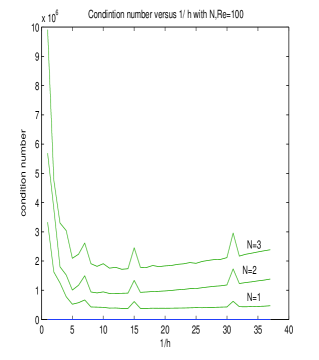
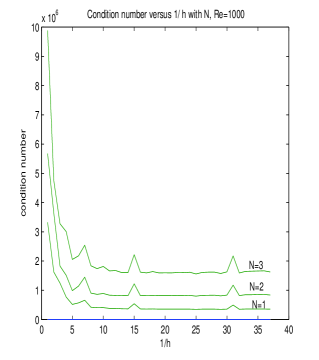
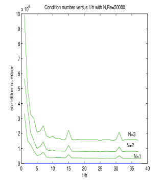
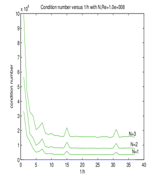
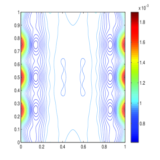
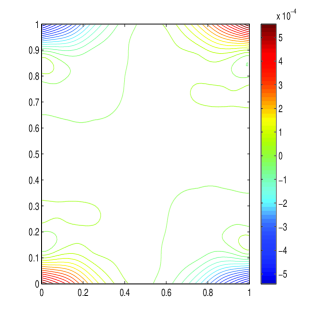
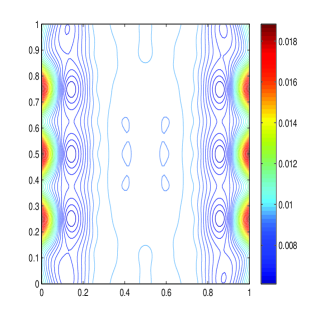
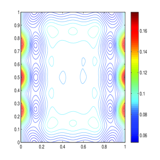
In Figures 1-4, we numerically show one of the striking benefits of the proposed schemes: the conditional number of the matrix of the corresponding matrix equation does not increase with the refining of the meshes for a wide range of Reynolds numbers. The well symmetric properties of the schemes should make contribution to this benefit. The $N$ denotes the degree of polynomial.

Figure 1: Conditional numbers vs $1/h$.

Figure 2: Conditional numbers vs $1/h$.

Figure 3: Conditional numbers vs $1/h$.

Figure 4: Conditional numbers vs $1/h$.

Example 5.2. For the convenience, we still choose the domain $\Omega=[0,1]\times[0,1]$; the source term $\bm f=(f_{1},f_{2})$, and the initial and boundary conditions are given as follows:

$$\left\{\begin{array}[]{l@{\quad} l}f_{1}(x,y,t)=e^{-\nu(x+y)t},\\ f_{2}(x,y,t)=sin(\nu(x+y)t);\end{array}\right.$$ (20)

$$\bm u(x,y,t)=\bm 0,\ \forall(x,y,t)\in\partial\Omega\times[0,T];\ \bm u(x,y,0)=\bm 0,\ \forall(x,y)\in\Omega.$$ (21)

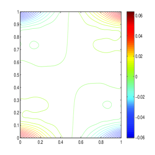
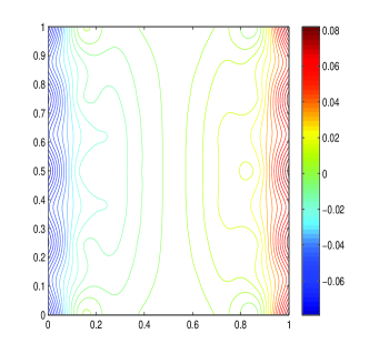
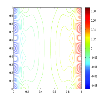
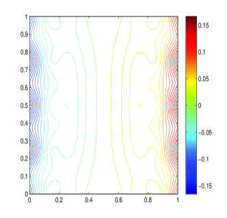
In this simulation, we use the first order polynomial, the spatial stepsize $h=1/8$, and the Reynolds number $Re=100$. Figures 5-13 show the contours of ${u_{1}}_{h}$, ${u_{2}}_{h}$, and $p_{h}(t)$ for the different times $t=0.001,\,0.01,\,0.1$.

Figure 5: The contour of ${u_{1}}_{h}$ with 001.

Figure 6: The contour of ${u_{2}}_{h}$ with t=0.001.

Figure 7: The contour of ${u_{1}}_{h}$ with t=0.01.

Figure 8: The contour of ${u_{2}}_{h}$ with t=0.01.

Figure 9: The contour of ${u_{1}}_{h}$ with t=0.1.

Figure 10: The contour of ${u_{2}}_{h}$ with t=0.1.

Figure 11: The contour of $p_{h}$ with t=0.001.

Figure 12: The contour of $p_{h}$ with t=0.01.

Figure 13: The contour of $p_{h}$ with t=0.1.

5 Conclusions

By carefully constructing the numerical fluxes, adding the penalty terms, and using the characteristic method to discretize the time derivative and nonlinear convective term, we design the effective LDG scheme to solve the time-dependent convection-dominated Navier-Stokes equations in $\mathbb{R}^{2}$. Besides the general advantages of the LDG scheme, the proposed scheme is theoretically proved or numerically verified to have the following benefits: 1) it is well symmetric, so easy to do theoretical analysis and numerical computation; 2) theoretically proved to unconditionally stable; 3) numerically verified to have the optimal convergence orders; 4) the conditional number of the matrix of the corresponding matrix equation does not increase with the refining of the meshes; 5) the scheme is efficient for a wide range of Reynolds numbers. The other possible variational formulation is presented in the Appendix.

Appendix

Here we present the other variational formulation for the time-dependent convection-dominated Navier-Stokes equations. We still use the characteristic method to discretize the time derivative and the nonlinear convection term. Multiplying the first, second, and third equation of (2) by arbitrary smooth test functions $\bm v,\bar{\bm\tau},q$, respectively, and integrating by parts over an arbitrary subset $E\in\mathscr{E}_{h}$ twice, we obtain

$$\left\{\begin{array}[]{l@{\quad} l}\int_{E}(\bm u_{t}+(\bm u\cdot\nabla)\bm u)\bm v-\int_{E}\sqrt{\nu}\nabla\cdot\bar{\bm\sigma}\bm v+\int_{\partial E}\sqrt{\nu}(\bar{\bm\sigma}-\bar{\bm\sigma}^{\ast})\cdot\bm v\cdot\bm n_{E}\\ +\int_{E}\nabla p\cdot\bm v-\int_{\partial E}(p-p^{\ast})\bm v\cdot\bm n_{E}=\int_{E}\bm f\bm v,\ \forall\bm v\in\bm V,\\ \\ \int_{E}\bar{\bm\sigma}:\bar{\bm\tau}+\int_{E}\sqrt{\nu}\nabla\cdot\bar{\bm\tau}\cdot\bm u-\int_{\partial E}\sqrt{\nu}\bm u^{\ast}\cdot\bar{\bm\tau}\cdot\bm n_{E}=0,\ \forall\bar{\bm\tau}\in\bm V^{2},\\ \\ -\int_{E}\nabla q\cdot\bm u+\int_{\partial E}q\bm u^{\ast\ast}\cdot\bm n_{E}=0,\ \forall q\in M,\end{array}\right.$$ (22)

where $\bm n_{E}$ is the outward unit normal to $\partial E$. Choosing the fluxes of $\bar{\bm\sigma}^{\ast},\bm u^{\ast},\bm u^{\ast\ast},p^{\ast}$ as:

$$\bar{\bm\sigma}^{\ast}=\{\{\bar{\bm\sigma}\}\},\ \ \bm u^{\ast}=\{\{\bm u\}\},\ \ p^{\ast}=\{\{p\}\},\ \ \bm u^{\ast\ast}=\{\{\bm u\}\},$$

leads to the second variational formulation:

$$\left\{\begin{array}[]{l@{\quad} l}\sum_{E\in\mathscr{E}_{h}}(\bm u_{t}+(\bm u\cdot\nabla)\bm u,\bm v)_{E}-\sum_{E\in\mathscr{E}_{h}}(\sqrt{\nu}\nabla\cdot\bar{\bm\sigma},\bm v)_{E}\\ +\sum_{e\in\mathscr{E}_{h}^{B}}(\sqrt{\nu}[\bar{\bm\sigma}],\{\{\bm v\}\}\otimes\bm n_{e})_{e}+\sum_{E\in\mathscr{E}_{h}}(\nabla p,\bm v)_{E}\\ -\sum_{e\in\mathscr{E}_{h}^{B}}([p],\{\{\bm v\}\}\cdot\bm n_{e})_{e}=\sum_{E\in\mathscr{E}_{h}}(\bm f,\bm v)_{E},\\ \\ \sum_{E\in\mathscr{E}_{h}}(\bar{\bm\sigma},\bar{\bm\tau})_{E}+\sum_{E\in\mathscr{E}_{h}}(\sqrt{\nu}\nabla\cdot\bar{\bm\tau},\bm u)_{E}\\ -\sum_{e\in\mathscr{E}_{h}^{B}}(\sqrt{\nu}[\bar{\bm\tau}],\{\{\bm u\}\}\otimes\bm n_{e})_{e}=0,\\ \\ -\sum_{E\in\mathscr{E}_{h}}(\nabla q,\bm u)_{E}+\sum_{e\in\mathscr{E}_{h}^{B}}([q],\{\{\bm u\}\}\cdot\bm n_{e})_{e}=0.\end{array}\right.$$ (23)

This formulation is unconditionally stable as the first one; and it is the strong formulation of the first one.

References

• [1] T. Arbogast, M.F. Wheeler, A characteristics-mixed finite element method for advection-dominated transport problems, SIAM J. Numer. Anal., 32(2) (1995) 404-424.
• [2] K. Boukir, Y. Maday, B. Métivet, A high order characteristics method for the incompressible Navier-Stokes equations, Comput. Methods Appl. Mech. Engrg., 116 (1994) 211-218.
• [3] K. Boukir, Y. Maday, B. Métivet, A high order characteristics//finite element method for the incompressible Navier-Stokes equations, Int. J. Numer. Methods Fluids, 25 (1997) 1421-1454.
• [4] B. Cockburn, C.-W. Shu, The local discontinuous Galerkin method for time-dependent convection-diffusion systems, SIAM J. Numer. Anal., 35(6) (1998) 2440-2463.
• [5] B. Cockburn, G. Kanschat, D. Schötzau, C. Schwab, Local discontinuous Galerkin methods for the Stokes System, SIAM J. Numer. Anal., 40(1) (2003) 319-343.
• [6] B. Cockburn, G. Kanschat, D. Schötzau, The local discontinuous Galerkin method for the Ossen equations, Math. Comput., 73 (2004) 569-593.
• [7] B. Cockburn, G. Kanschat, D.Schötzau, A locally conservative LDG method for the incompressible Navier-Stokes equations, Math. Comput., 74 (2005) 1067-1095.
• [8] B. Cockburn, G. Kanschat, D. Schötzau, A note on discontinuous Galerkin divergence-free solutions of Navier-Stokes equations, J. Sci. Comput., 31 (2007) 61-73.
• [9] P. Castillo, B. Cockburn, I. Perugia, D. Schötzau, An apriori error analysis of the local discontinuous Galerkin method for elliptic problems, SIAM J. Numer. Anal., 38 (2001) 1676-1706.
• [10] P. Castillo, B. Cockburn, C. Schwab, Optimal apriori error analysis for the hp-version of the local discontinuous Galerkin method for convection-diffusion problems, Math. Comput., 71 (2002) 455-478.
• [11] V. Girautl, R. Scott, A quasi-local interpolation operator preserving the discrete divergence, Calcolo, 40 (2003) 1-19.
• [12] V. Girautl, B. Rivière, M.F. Wheeler, A splitting method using discontinuous Galerkin for the transient incompressible Navier-Stokes equations, ESAIM: M2AN, 39 (2005) 1115-1147.
• [13] V. Girautl, P. Raviart, Finite Element Methods for Navier-Stokes Equations: Theory and Algorithms, Volume 5 of Springer Series in Computational Mathematics, (Springer-Verlag, Berlin, 1986).
• [14] B. Rivière, V. Girault, Discontinuous finite element methods for incompressible flows on subdomains with non-matching interfaces, Comput. Meth. Appl. Mech. Engrg., 195 (2006) 3274-3292.
• [15] B. Rivière, Discontinuous Galerkin Methods for Solving Elliptic and Parabolic Equations: Theory and Implementation, Society for Industrial and Applied Mathematics, (SIAM, 1999).
• [16] R. Temam, Navier-Stokes Equations: Theory and Numerical analysis, North-Holland-Amsterdam. New York. Oxford, (Elsevier Science Publishers B.V., 1984).
• [17] F. Bassi and S. Rebay, A high-order accurate discontinuous finite elemnet method for the numerical solution of the compressible Navier-Stokes equations, J. Comput. Phys., 131 (1997) 267-279.
• [18] W.H. Deng, Finite element method for the space and time fractional Fokker-Plank equations, SIAM J. Numer. Anal, 47(1) (2008) 204-226.
• [19] W.H. Deng, J.S. Hesthaven, Local discontinuous Galerkin methods for fractional diffusion equations, ESAIM: M2AN, 47 (2013) 1845-1864.
• [20] R.H. Nochetto, J.-H. Pyo, The Gauge-Uzawa finite element method. Part I: the Navier-Stokes equations, SIAM J. Numer. Anal., 43(3) (2005) 1043-1068 .
• [21] Z.X. Chen, Characteristic mixed discontinuous finite element methods for advection-dominated diffusion problems, Comput. Methods Appl. Mech. Engrg., 191 (2002) 2509-2538.
• [22] P.G. Ciarlet, The Finite Element Method for Elliptic Problems, North-Holland-Amsterdam. New York. Oxford, (Elsevier Science Publishers B.V., 1978).
• [23] Y. He, A fully discrete stabilized finite-element method for the time-dependent Navier-Stokes problem, IMA Journal of Numerical Analysis 23 (2003) 665-691.