Zero-Delay Joint Source-Channel Coding for a Multivariate Gaussian on a Gaussian MAC

Abstract

In this paper, communication of a Multivariate Gaussian over a Gaussian Multiple Access Channel is studied. Distributed zero-delay joint source-channel coding (JSCC) solutions to the problem are given. Both nonlinear and linear approaches are discussed. The performance upper bound (signal-to-distortion ratio) for arbitrary code length is also derived and Zero-delay cooperative JSCC is briefly addressed in order to provide an approximate bound on the performance of zero-delay schemes. The main contribution is a nonlinear hybrid discrete-analog JSSC scheme based on distributed quantization and a linear continuous mapping named Distributed Quantizer Linear Coder (DQLC). The DQLC has promising performance which improves with increasing correlation, and is robust against variations in noise level. The DQLC exhibits a constant gap to the performance upper bound as the signal-to-noise ratio (SNR) becomes large for any number of sources and values of correlation. Therefore it outperforms a linear solution (uncoded transmission) in any case when the SNR gets sufficiently large.

I Introduction

In this paper we investigate joint source-channel coding (JSCC) for a multipoint-to-point problem, where multiple memoryless and inter-correlated Gaussian sources are transmitted distributedly over a memoryless Gaussian multiple access channel (GMAC) without multiplexing. There are mainly two cases to consider for this network: 1) Recovery of the common information shared by all sources. 2) Recovery of each individual source. In Case 1), when the transmit power of all sources are equal, the distortion lower bound can be achieved by a simple zero-delay linear mapping, often referred to as uncoded transmission [1].

In case 2) both common information as well as the individual variations of each source are reconstructed at the receiver. The bivariate case (two sources) was treated in [2] for arbitrary codeword length. The authors proposed a nonlinear hybrid JSCC scheme that superimposes a rate optimal (infinite dimensional) vector quantizer with uncoded transmission. This hybrid scheme was shown to achieve the distortion lower bound at high and low channel signal-to-noise ratio (SNR), while a small gap remains for other SNR. Contrary to case 1), optimality of uncoded transmission is restricted (to low SNR in general), and infinite complexity and delay JSCC are required to get close to the distortion lower bound in general. The bivariate case was also treated in [3], where a zero-delay (single letter) constraint was imposed in order to provide simple low complexity and possibly implementable solutions to the problem. Two zero-delay nonlinear schemes were proposed, one discrete scheme and one hybrid discrete-analog scheme. Both schemes perform well and can improve significantly on uncoded transmission when the channel signal-to-noise ratio (SNR) is sufficiently large. Nevertheless, there remains a constant gap to the distortion lower bound for all SNR due to the zero-delay constraint.

The main contribution of this paper is to provide a nonlinear zero-delay JSCC solution for the multivariate version of case 2), since there to our knowledge exists few, if any, results on this in the literature. We generalize the hybrid discrete-analog scheme from [3] (named SQLC) to the multivariate case. The proposed scheme is named DQLC since it consists of distributed quantizers and a linear continuous mapping. The main advantage of DQLC is that it provides a simple JSCC solution to the problem that can significantly outperform uncoded transmission under sufficiently large channel SNR.

To assess the performance of DQLC, the distortion lower bound for the problem under consideration is derived. Since this lower bound assumes arbitrary codelength, one must expect a significant backoff from it when assessing performance of a zero-delay JSCC scheme. To provide indications on the bound for zero-delay distributed schemes, and thereby a better measure on how well the DQLC perform, known zero-delay schemes with cooperative encoders are addressed. It is also shown that DQLC exhibits a constant gap to the distortion lower bound (or performance upper bound, the bound on signal-to-distortion ratio) as SNR $\rightarrow\infty$. This gap increases somewhat with the number of of sources, but remains bounded as the number of sources becomes large. Since uncoded transmission has a leveling off effect at high SNR, DQLC will therefore outperform uncoded transmission for any number of sources when the SNR is sufficiently large.

The paper is organized as follows: In Section II, a problem formulation is given and the distortion lower bound is derived. Zero-delay cooperative encoding and uncoded transmission are also introduced. In Section III the DQLC is introduced and its distortion is derived mathematically. It is further shown that DQLC exhibits a constant gap to distortion lower bound as SNR$\rightarrow\infty$. In Section IV we concentrate on the 3 source case and optimize the DQLC for general SNR. Its performance is compared to the derived bounds and uncoded transmission. A summary and brief discussion are given in Section V.

Note that some of the results in this paper have previously been published in [4].

II Problem statement and bounds

Fig. 1 depicts the communication system under consideration.

Figure 1: Network under consideration. A multivariate Gaussian is communicated on a Gaussian MAC with separate (distributed) encoders.

II-A Problem statement

The sources are memoryless discrete time, continuous amplitude, zero mean Gaussian random variables $x_{1},...,x_{M}$, where the model $x_{m}=s+w_{m},m\in\{1,...,M\}$ is considered. That is, the sources share a common information $s\sim\mathcal{N}(0,\sigma_{s}^{2})$, while each source also has an individual component $w_{m}\sim\mathcal{N}(0,\sigma_{w_{m}}^{2})$. A simplified scenario $\sigma_{w_{1}}=\sigma_{w_{2}}=\cdots=\sigma_{w_{M}}$ is assumed here, which implies that $\sigma_{x_{1}}=\sigma_{x_{2}}=\cdots=\sigma_{x_{M}}=\sigma_{x}$, making it easier to derive theoretical expressions that can be analyzed further. The correlation between any two sources is then $\rho_{ij}=\mathbf{E}\{x_{i}x_{j}\}/\sigma_{x}^{2}=\rho_{x},\forall i,j$, resulting in a simple covariance matrix $K_{\mathbf{x}}=\mathbf{E}\{\mathbf{x}\mathbf{x}^{T}\}$ with $\sigma_{x}^{2}$ on the diagonal and $\sigma_{x}^{2}\rho_{x}$ in every off-diagonal element, and eigenvalues $\lambda_{1}=\sigma_{x}^{2}((M-1)\rho_{x}+1)$ and $\lambda_{i}=\sigma_{x}^{2}(1-\rho_{x})$, $i=2,\cdots,M$. Note that the schemes presented in this paper can be applied for any case of unequal correlations $\rho_{ij}$. The mathematical analysis becomes more complicated, however.

Each encoder consists of a memoryless encoding function $y_{m}=f_{m}(x_{i}),m\in\{1,...,M\},$ and its output is transmitted over GMAC with additive noise $n\sim\mathcal{N}(0,\sigma_{n}^{2})$. The received signal is

$$z=\sum_{m=1}^{M}f_{m}(x_{m})+n\in\mathbb{R}.$$ (1)

At the receiver the functions $g_{m}(z),m\in\{1,...,M\}$, produce the estimates $\hat{x}_{1},...,\hat{x}_{M}$ from the channel output $z$. We define the end-to-end distortion $D$ as the mean-squared-error (MSE) averaged over all source symbols

$$D=\frac{1}{M}\left(\mathbf{E}\{|x_{1}-\hat{x}_{1}|^{2}\}+\cdots+\mathbf{E}\{|x_{M}-\hat{x}_{M}|^{2}\}\right).$$ (2)

The average transmit power for node $m$ is defined as $P_{m}=\mathbf{E}\{f_{m}(x_{m})^{2}\}$. We further assume ideal Nyquist sampling and an ideal Nyquist channel, where the sampling rate of each source is the same as the signalling rate of the channel. We also assume ideal synchronization and timing between all nodes. Our design objective is to find the $f_{m}$ and $g_{m}$ that minimizes $D$. The DQLC encoders are asymmetric, where $P_{1}\geq P_{2}\geq\cdots\geq P_{M}$. Therefore, an average transmit power constraint $P=(P_{1}+P_{2}+\cdots P_{M})/M$ is considered.

II-B Distortion lower bound

When no collaboration is allowed among the encoders, the achievable distortion bound is unknown. One can, however, derive a lower bound by considering the ideal scenario with full collaboration among all encoders at no additional cost. This scenario is then a point-to-point communication problem, where the distortion lower bound can be determined by equating the rate-distortion function for an $M$ dimensional Gaussian source to the rate of the GMAC. The following proposition quantifies this bound.

Proposition 1

The distortion lower bound for the network in Fig. 1, is in the symmetric case $D_{1}=D_{2}=\cdots=D_{M}=D$ with transmit power $P_{1}=P_{2}=\cdots=P_{M}=P$ and correlation $\rho_{ij}=\rho_{x}$, $\forall i,j$, given by

$${D}\geq\begin{cases}\sigma_{x}^{2}\left(1-\frac{P(1+(M-1)\rho_{x})^{2}}{P(M^{2}\rho_{x}+M(1-\rho_{x}))+\sigma_{n}^{2}}\right)&\frac{P}{\sigma_{n}^{2}}\in\big{(}0,\frac{\rho_{x}}{1-\rho_{x}^{2}}\big{]},\vspace{0.3cm}\\ \sigma_{x}^{2}\sqrt[M]{\frac{\big{(}1+(M-1)\rho_{x}\big{)}(1-\rho_{x})^{M-1}\sigma_{n}^{2}}{P\big{(}M+M(M-1)\rho_{x}\big{)}+\sigma_{n}^{2}}},&\frac{P}{\sigma_{n}^{2}}>\frac{\rho_{x}}{1-\rho_{x}^{2}}.\end{cases}$$ (3)

Proof:

Let $R^{*}$, $D^{*}$ and $P^{*}$ denote optimal rate, distortion and power respectively. Assuming full collaboration, the $M$ sources can be considered as a Gaussian vector source of dimension $M$. From [5]

$$D^{*}(\theta,M)=\frac{1}{M}\sum_{i=1}^{M}\min[\theta,\lambda_{i}],$$ (4)

$$R^{*}(\theta,M)=\frac{1}{M}\sum_{i=1}^{M}\max\left[0,\frac{1}{2}\log_{2}\frac{\lambda_{i}}{\theta}\right],$$ (5)

where $\lambda_{i}$ is the $i$-th eigenvalue of the covariance matrix $K_{\mathbf{x}}$.

Assuming that all $M$ encoders transmit at the same power and that the correlation between the encoder outputs, $y_{m}$, are equal to $\rho_{x}\geq 0$, the following Lemma results

Lemma 1

The channel capacity per source symbol is

$$C=\frac{1}{2M}\log_{2}\bigg{(}1+\frac{MP^{*}(1+(M-1)\rho_{x})}{\sigma_{n}^{2}}\bigg{)}.$$ (6)

Proof:

Let $Y_{i,k}$ be the i’th encoder output at time instant $k$. Using Lemma C.2 and Theorem C.1 from [2], it can be shown that:

$$\frac{1}{n} \sum_{k=1}^{n}\mathbf{E}\left[\left(\sum_{i=1}^{M}Y_{i,k}\right)^{2}\right]=\sum_{i=1}^{M}\left(\sum_{k=1}^{n}\mathbf{E}[Y_{i,k}^{2}]\right)+$$

$$\ \ \ \ \ \ \ \ \ \ \ \ 2\sum_{i,j=1,i\neq j}^{M}\left(\frac{1}{n}\sum_{k=1}^{n}\mathbf{E}[Y_{i,k}Y_{j,k}]\right)$$

$$\stackrel{{\scriptstyle(a)}}{{\leq}}MP+2\rho_{x}\sum_{i,j=1,i\neq j}^{M}\left(\frac{1}{n}\sum_{k=1}^{n}\sqrt{\mathbf{E}[Y_{i,k}^{2}]}\sqrt{\mathbf{E}[Y_{j,k}^{2}]}\right)$$

$$\stackrel{{\scriptstyle(b)}}{{\leq}}MP+2\rho_{x}\sum_{i,j=1,i\neq j}^{M}\left(\frac{1}{n}\sqrt{\sum_{k=1}^{n}\mathbf{E}[Y_{i,k}^{2}]}\sqrt{\sum_{k=1}^{n}\mathbf{E}[Y_{j,k}^{2}]}\right)$$

$$\leq MP+2\rho_{x}\dbinom{M}{2}P$$ (7)

where $(a)$ comes from [2, Lemma C.2] given $\rho_{x}\geq 0$, and $(b)$ is the Cauchy-Schwartz inequality. The resulting channel capacity is then (6). ∎

Now equate $R^{*}$ from (5) with $C$ in (6) and calculate the corresponding power $P^{*}$. We get $D\geq D^{*}(\theta,M)$ with $D^{*}$ given in (4) and

$$P=P^{*}(\theta,M)=\sigma_{n}^{2}\frac{\prod_{1}^{M}{\max[\lambda_{i}/\theta,1]}-1}{M+M(M-1)\rho_{x}}$$ (8)

The max and min in (4) and (8) depends on $\rho_{x}$ and the SNR. Since the special case $\rho_{ij}=\rho_{x},\forall i,j$ is treated, there are two cases to consider: Only the first eigenvalue $\lambda_{1}$ is to be represented (the common information) and all eigenvalues, $\lambda_{i},i\in[1,\cdots M]$, are to be represented. The validity of these two cases is the same as in [2], i.e. SNR=$P/\sigma_{n}^{2}\leq\rho_{x}/(1-\rho_{x}^{2})$ and SNR=$P/\sigma_{n}^{2}>\rho_{x}/(1-\rho_{x}^{2})$ respectively. If one solve (8) with respect to $\theta$ for these two cases and insert the result in (4), the bound (3) results. ∎

Note that (3) becomes a bound for an average transmit power constraint by setting $P=(P_{1}+P_{2}+\cdots+P_{M})/M$.

II-C Zero-delay JSCC with collaborating encoders

Since collaboration makes it possible to construct a larger set of encoding operations, including all distributed strategies, the performance of distributed coding schemes is upper-bounded by those that allow collaboration. Optimal zero-delay collaborative schemes therefore serve as a tighter bound for single letter schemes compared to the ones without restrictions on codeword length.

In the case of zero delay, the corresponding optimal collaborative encoding operation is the mapping $\mathbb{R}^{M}\rightarrow\mathbb{R}$ from source to channel space, which minimizes $D$ at a given power constraint. It has not yet been determined how such a mapping should be constructed in order to perform optimally. One can anyway get an indication on how a scheme with collaborative encoders performs from schemes that are known to operate close to the distortion lower bound. Examples on known schemes with excellent performance are Shannon-Kotel’nikov mappings (S-K mappings) [6, 7, 8, 9, 10] and Power Constrained Channel Optimized Vector Quantizers (PCCOVQ) [11, 12]. PCCOVQ can be considered similar to S-K mappings when the number of centroids is large and is therefore referred to as S-K mappings in the following. S-K mappings have previously been optimized for memoryless Gaussian sources and channels when $M$ source symbols are transmitted on $N$ channel uses [6, 8, 7, 9, 10, 11, 12].

For the problem at hand, by treating the collaborative encoders as one, and the $M$ sources as components of a Gaussian vector source, S-K mappings with $N=1$ can be applied directly. S-K mappings can not be applied to the distributed case, however, as their operation would require knowledge of all source symbols simultaneously at each encoder [7, 6, 8, 11, 12].

II-D Distributed linear JSCC: uncoded transmission

A simple way to construct zero-delay distributed encoders is to let each sensor node scale its observations to satisfy the power constraint, i.e. $f_{m}(x_{m})=x_{m}\sqrt{{P}/{\sigma_{x}^{2}}}$. With equal transmit power, the received signal becomes

$$z=\sqrt{\frac{P}{\sigma_{x}^{2}}}\left(Ms+\sum_{m=1}^{M}w_{m}\right)+n.$$ (9)

At the receiver, MMSE decoding given by $\hat{x}_{m}=(\mathbf{E}[x_{m}z]/\mathbf{E}[z^{2}])z$, is applied. One can show that the resulting end-to-end distortion becomes

$$\begin{split}D&=\sigma_{x}^{2}-\frac{\mathbf{E}[x_{i}z]^{2}}{\mathbf{E}[z^{2}]}\\ &=\sigma_{x}^{2}\left(1-\frac{P(1+(M-1)\rho_{x})^{2}}{P(M^{2}\rho_{x}+M(1-\rho_{x}))+\sigma_{n}^{2}}\right).\end{split}$$ (10)

Considering (3), one can see that a linear mapping is optimal when $P/\sigma_{n}^{2}\leq\rho_{x}/(1-\rho_{x}^{2})$, i.e. when only the common information $s$ can be reconstructed.

III Distributed nonlinear JSCC: DQLC

In order to get closer to the bound in (3) than uncoded transmission when $P/\sigma_{n}^{2}>\rho_{x}/(1-\rho_{x}^{2})$, nonlinear mappings are needed. A zero-delay hybrid discrete-analog scheme, DQLC, where encoders 1 to $M-1$ are amplitude limited scalar quantizers and encoder $M$ consist of a limiter followed by scaling, is presented here.

III-A Formulation of Encoders and Decoders

Encoder $m$, $m\in[1,\ldots,M-1]$, first quantizes $x_{m}$, then limits the quantizer output to a certain range $\pm\kappa_{m}$, where $\kappa_{m}\in\mathbb{R}^{+}$, and further attenuates the result by $\alpha_{m}$. That is $f_{m}(x_{m})=\alpha_{m}\ell_{\pm\kappa_{m}}[q_{\Delta_{m}}(x_{m})]$. $q_{\Delta_{m}}(x_{m})$ is a uniform midrise or midthread quantizer, where $q_{i_{m}}$ denotes centroid no. $i$ of quantizer $m$. Encoder $M$ only limits $x_{M}$ to $\pm\kappa_{M}$, then attenuates the result by $\alpha_{M}$. That is $f_{M}(x_{M})=\alpha_{M}\ell_{\pm\kappa_{M}}[x_{M}]$. The received signal becomes

$$\begin{split}&z=\sum_{m=1}^{M-1}\alpha_{m}(\ell_{\pm\kappa_{m}}[q_{\Delta_{m}}(x_{m})])+\alpha_{M}(\ell_{\pm\kappa_{M}}[x_{M}])+n.\end{split}$$ (11)

In the following we choose $\alpha_{1}=1$ and $\kappa_{1}=\infty$.

An example for $M=3$ is shown in Fig. 2.

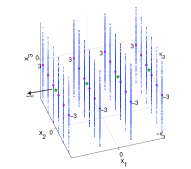
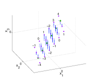
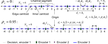
Figure 2: DQLC for $M=3$. Source space for: (a) $\rho_{x}=0$. (b) $\rho_{x}=0.95$. (c) Channel space. Here $\kappa_{2}=4$ when $\rho_{x}=0$ and $\kappa_{2}=5$ when $\rho_{x}=0.95$.

The encoders first create the segments in source space as shown in Fig. 2 ($\rho_{x}=0$) and 2 ($\rho_{x}=0.95$) through quantization and limitation. These segments are attenuated by $\alpha_{m}$ in such a way that the channel space structure shown in Fig. 2 results when GMAC sums over all encoder outputs. To obtain this structure, $\alpha_{1}>\alpha_{2}>\cdots>\alpha_{M}$. From Fig. 2 one can see how DQLC is affected by correlation. As $\rho_{x}$ increases, the joint pdf $p_{\mathbf{x}}(x_{1},\cdots,x_{M})$ narrows along all its minor axes, effectively limiting each source segment. The operation $\ell_{\pm\kappa_{m}}$ then becomes obsolete. This effect results in reduced distortion. As $\rho_{x}\rightarrow 1$ one can let $\Delta_{m}\rightarrow 0$, $\alpha_{m}\rightarrow 1$ and $\kappa_{m}\rightarrow\infty,\forall m$, and the DQLC becomes equivalent to uncoded transmission.

To cancel interference at the receiver, sequential decoding is used: First an estimate of source $1$ is made. This estimate is then subtracted from the channel output to estimate source $2$, and so on. In order to make the correct decision on the output from quantizer $m$, one must take into account that the midpoint of each channel segment changes with $\rho_{x}$ (like $d_{1}$ and $d_{2}$ shown in Fig. 2). Consider source 1: the first order moment of $p(\alpha_{2}x_{2},\ldots,\alpha_{M}x_{M}|x_{1}=q_{i_{1}})$ must be determined. Consider a sub-division of $\mathbf{y}=[x_{1}\hskip 5.69046pt\cdots\hskip 5.69046pt\alpha_{M}x_{M}]$ into $\mathbf{y}_{a}=[\alpha_{2}x_{2}\hskip 5.69046pt\cdots\hskip 5.69046pt\alpha_{M}x_{M}]^{T}$ and $\mathbf{y}_{b}=x_{1}$. By sub-dividing the covariance matrix $K_{\mathbf{y}}=E\{\mathbf{y}\mathbf{y}^{T}\}$ according to (45), Theorem 1 in the Appendix gives $\mathbf{E}\{\alpha_{2}x_{2},\ldots,\alpha_{M}x_{M}|x_{1}\}=\rho_{x}x_{1}\begin{bmatrix}\alpha_{2}&\cdots&\alpha_{M}\end{bmatrix}^{T}$. When the transformed sources are summed together, centroids of encoder 1 are shifted by the sum of all first order moments. When source 1 is detected, one can subtract it from $z$ then use the same argument as above for source 2, and so on. Let $N_{q_{m}}$ denote the number of centroids for quantizer $m$. The estimate of sources $m\in[1,M-1]$ becomes

$$\begin{split}&g_{m}(z)=\arg\min_{q_{i_{m}},i_{m}\in[1,N_{q_{m}}]}\\ &\bigg{\|}\bigg{(}z-\sum_{l=1}^{m-1}\alpha_{l}g_{l}(z)\bigg{)}-q_{i_{m}}\cdot\bigg{(}\alpha_{m}+\rho_{x}\sum_{k=m+1}^{M}\alpha_{k}\bigg{)}\bigg{\|}^{2}.\end{split}$$ (12)

The estimate of the $M$’th source is then found from

$$g_{M}(z)=\beta\bigg{(}z-\sum_{m=1}^{M-1}\alpha_{m}g_{m}(z)\bigg{)},$$ (13)

where $\beta$ is a scaling factor. The MSE is further minimized by computing

$$\hat{x}_{m}=[x_{m}|g(x_{1}),\cdots,g(x_{M})],\hskip 5.69054ptm\in[1,\cdots,M]$$ (14)

The optimal parameters $\alpha_{m}$, $\Delta_{m}$ and $\kappa_{m}$ need to be found. To ensure that each source is uniquely decodable, the relation between the $\alpha$’s must be $1=\alpha_{1}\geq\alpha_{2}\geq\alpha_{3}\geq\cdots\geq\alpha_{M}>0$. When optimizing DQLC, we look at the number of centroids of encoder $m$, $N_{q_{m}}$, instead of the clipping $\kappa_{m}$ (except for encoder $M$). The parameters $\overrightarrow{\Delta}=[\Delta_{1},\cdots,\Delta_{M-1}]^{T}$, $\overrightarrow{N_{q}}=[N_{q_{2}},\cdots,N_{q_{M-1}}]^{T}$, $\overrightarrow{\alpha}=[\alpha_{2},\cdots,\alpha_{M}]^{T}$, $\beta$ and $\kappa_{M}$ are optimized for an average power constraint $P$. With $D$ as in (2)

$$\min_{\overrightarrow{\Delta},\overrightarrow{N_{q}},\overrightarrow{\alpha},\beta,\kappa_{M}:\sum_{m=1}^{M}P_{m}\leq MP}D.$$ (15)

To calculate $D$ and $P_{m}$, the channel output pdf is needed.

III-B Calculation of channel output pdf

To determine the relevant pdf, $\kappa_{m}$, $\Delta_{m}$ and $\alpha_{m}$ must be chosen so that channel segments do not overlap (the configuration in Fig. 2). Since the outputs of encoders 1 to $M-1$ are discrete, their distributions can be expressed by point probabilities, which are straight forward to calculate. For the output of encoder $M$, two cases must be considered: 1) $\rho_{x}$ close enough to 0 for $\ell_{\pm\kappa_{M}}[x_{M}]$ to be significant. 2) $\rho_{x}$ so close to $1$ that $p_{\mathbf{x}}(x_{1},\cdots,x_{M})$ effectively limits the segments so that $y_{M}=f_{M}(x_{M})\approx\alpha_{M}x_{M}$.

Case 1): The whole range of $y_{M}=f_{M}(x_{M})$ is now represented on each channel segment, as can be seen by studying the blue lines in Fig. 2 and 2. The pdf of encoder $M$ at the channel output is determined by assuming that sources $1$ to $M-1$ are subtracted. Then the same analysis as for the $M=2$ case in [3] can be applied. With the mean given by

$$\mu=q_{i_{M-1}}(\alpha_{M-1}+\rho_{x}\alpha_{M})+\sum_{m=1}^{M-2}q_{i_{m}},$$ (16)

the same arguments as in [3] lead to

$$\begin{split}&p_{z_{M}(\overrightarrow{i}_{m})}(z_{M})_{\kappa_{M}}=\frac{1}{\Sigma}\int_{-\alpha_{M}\kappa_{M}}^{\alpha_{M}\kappa_{M}}e^{-\frac{\alpha_{M}^{2}\sigma_{x}^{2}(z_{M}-\mu-y)^{2}+\sigma_{n}^{2}y^{2}}{2\alpha_{M}^{2}\sigma_{x}^{2}\sigma_{n}^{2}}}\mbox{d}y\\ &+p_{o}\big{(}p_{n}(z_{M}-\mu-\alpha_{M}\kappa_{M})+p_{n}(z_{M}-\mu+\alpha_{M}\kappa_{M})\big{)},\end{split}$$ (17)

where $p_{o}=Pr\{x_{M}\geq\kappa_{M}\}$, $\Sigma=2\pi\alpha_{M}\sigma_{x}\sigma_{n}$, $p_{n}$ is the noise pdf, and $z_{M}$ denotes the received signal when sources $1\ldots M-1$ are subtracted. Fig. 4 shows this pdf when $\mu=0$.

Case 2): When $\rho_{x}$ is close to 1, each source segment, and therefore also each channel segment, will no longer be equivalent but contain somewhat different (but intersecting) ranges of $y_{M}$ (this also applies to sources 2 to $M-1$ given the others). This can be seen by studying the blue lines in Fig. 2 and Fig. 2. One can now assume that $y_{M}=f_{M}(x_{M})\approx\alpha_{M}x_{M}$. To determine the relevant pdf, $p(y_{M}|q_{i_{1}},\ldots,\alpha_{M-1}q_{i_{M-1}})$, after summation over GMAC must be found. Consider a sub-division of $\mathbf{y}=[x_{1}\hskip 5.69046pt\cdots\hskip 5.69046pt\alpha_{M}x_{M}]$ into $\mathbf{y}_{a}=\alpha_{M}x_{M}$ and $\mathbf{y}_{b}=[x_{1}\hskip 5.69046pt\alpha_{2}x_{2}\hskip 5.69046pt\cdots\hskip 5.69046pt\alpha_{M-1}x_{M-1}]^{T}$. By sub-dividing the covariance matrix $K_{\mathbf{y}}=\mathbf{E}\{\mathbf{y}\mathbf{y}^{T}\}$ according to (45), Theorem 1 in the Appendix gives the second order moment

$$\begin{split}&\Sigma_{aa\cdot b}=\sigma_{x}^{2}\alpha_{M}^{2}\bigg{(}1-\frac{(M-1)\rho_{x}^{2}}{1+(M-2)\rho_{x}}\bigg{)}.\end{split}$$ (18)

By inserting (18) into (46) (in the Appendix) and (16) for the mean, the wanted pdf results. After addition of noise, the resulting pdf is found by the convolution $p(y_{M}|q_{i_{1}},\ldots,\alpha_{M-1}q_{i_{M-1}})\ast p_{n}(n)$ [13, 181-182], and thus

$$p_{z_{M}(\overrightarrow{i}_{m})}(z_{M})_{\gamma_{M}}=\frac{1}{\sqrt{2\pi\big{(}\sigma_{n}^{2}+\Sigma_{aa\cdot b}\big{)}}}{e^{-\frac{1}{2}\frac{(\mu-z_{M})^{2}}{\sigma_{n}^{2}+\Sigma_{aa\cdot b}}}}.$$ (19)

The validity of (17) and (19) must be determined. Since the correlation between any two sources is assumed to be the same, one can focus on the $x_{M},x_{M-1}$ plane. Fig. 3 provides a geometrical picture for the following discussion.

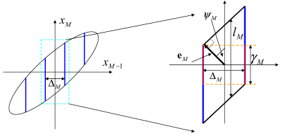
Figure 3: DQLC seen in the $x_{M-1},x_{M}$-plane when $\rho_{x}=0.95$. The expanded rectangle on the right can be applied to calculate anomalous errors for source $M$.

Let $l_{M}$ denote the length of the portion of the $x_{M}$ axis that contains the significant probability mass given $x_{M-1}$ (or $q_{i_{M-1}}$). $l_{M}=2\sqrt{\vartheta}\|\mathbf{e}_{M}\|=2b_{M}\sqrt{\vartheta\lambda_{M}}$, where $\|\mathbf{e}_{M}\|=b_{M}\sqrt{\lambda_{M}}$ denotes the length of the minor axis of the ellipse depicted (the source space). $b_{M}$ ($\approx 4$) is a parameter determining the width of the ellipse shown, and should be chosen so that the significant probability mass is within this ellipse. $\vartheta=(l_{M}/(2\|\mathbf{e}_{M}\|))^{2}$ depends on $\rho_{x}$: If $\rho_{x}=0$, then $\vartheta=1$ since the source space is rotationally invariant (a sphere). If $\rho_{x}>\approx 0.7$ then $\vartheta\approx 1/\cos^{2}(\psi_{M})=1/\cos^{2}(\pi/4)=2$. That is, $\vartheta\in[1,2]$, depending on $\rho_{x}$. (17) is valid when $l_{M}>2\kappa_{M}$ while (19) is valid when $l_{M}\leq 2\kappa_{M}$.

The total channel output pdf is given by

$$\begin{split}p_{z}(z)=\sum_{\overrightarrow{i}_{m}}Pr\{\overrightarrow{i}_{m}\}p_{z_{M}|\overrightarrow{i}_{m}}.\end{split}$$ (20)

$p_{z_{M}|\overrightarrow{i}_{m}}$ is given by  (19) or (17) depending on whether $l_{1}>2\kappa$ or not. $\overrightarrow{i}_{m}=[i_{1},i_{2},\cdots,i_{M-1}]$, and $Pr\{\overrightarrow{i}_{m}\}=Pr\{q_{i_{1}}\}Pr\{q_{i_{2}}|q_{i_{1}}\}\cdots Pr\{q_{i_{M-1}}|q_{i_{1}},\cdots,q_{i_{M-2}}\}$. Fig. 4 shows an example of the channel output pdf when $M=3$ at 30 dB channel SNR.

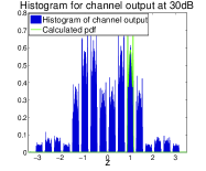
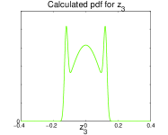
Figure 4: Channel output pdf when $M=3$. (a) Histogram where 4 centroids of encoder 1 is in use and $N_{q_{2}}=4$. The green curve shows (17) when the first positive centroid (index 1) are transmitted for both encoder 1 and 2. (b) (17) shown centered at the origin ($\mu=0$), that is when centroids for encoders 1 and 2 are given.

III-C Distortion and Power calculation

To calculate the distortion, we use an approach similar to that in [3], where the total distortion is divided into several contributions.

III-C1 Distortion and power for source $M$

The distortion for source $M$ can be divided into three contributions: clipping distortion, anomalous distortion and channel distortion.

Clipping distortion: At encoder $M$ we only have distortion from limitation, $\bar{\varepsilon}_{\kappa_{M}}^{2}$, an event with probability $Pr\{|x_{M}|>\kappa_{M}\}$ and error $(x_{M}-\kappa_{M})^{2}$:

$$\bar{\varepsilon}_{\kappa{{}_{M}}}^{2}=2\int_{\kappa_{M}}^{\infty}(x_{M}-\kappa_{M})^{2}p_{x}(x_{M})\mbox{d}x_{M}.$$ (21)

The distortion from channel noise can be split into two contributions: Channel distortion and anomalous distortion.

Anomalous distortion: results from a threshold effect (see e.g. [14] or [15]) and occurs every time the centroid for one or several of quantizers 1 to $M-1$ is erroneously selected. This error leads to a ”jump” from one channel segment to another (see Fig. 2) for source $M$, resulting in large decoding errors. In the worst case scenario ($\rho_{x}=0$) large positive and negative values are interchanged. The anomalous distortion is difficult to calculate exactly. We therefore look at an approximation valid around the optimal operation of DQLC. Note that jumps among centroids of in encoder 1 are most fatal since this leads to anomalous distortion for all other sources. Jumps among centroids of encoder 2 lead to anomalous errors for sources 3 to $M$, and so on. Therefore, the probability for jumps among centroids of quantizer 1 to $M-2$ should be at least as small as the probability for jumps among centroids of quantizer $M-1$. By assuming that encoders 1 to $M-1$ are constructed correctly, one can calculate an upper bound on anomalous distortion for source $M$ by considering jumps among centroids of quantizer $M-1$ only. We are then in the same situation as the $M=2$ case in [3], and can calculate the anomalous errors from the $x_{M-1},x_{M}$ plane shown in Fig. 3. Two cases must be considered: $l_{M}>2\kappa_{M}$ and $l_{M}\leq 2\kappa_{M}$.

Assume first $l_{M}>2\kappa_{M}$: anomalous errors happen whenever $y_{M}+n\geq d_{M-1}/2=\Delta_{M-1}(\alpha_{M-1}+\alpha_{M}\rho_{x})/2$ (see $M=3$ case in Fig. 2), i.e. the probability for anomalies are

$$\begin{split}p_{thM}&=2\int_{\frac{\Delta_{M-1}}{2}(\alpha_{M-1}+\alpha_{M}\rho_{x})}^{\infty}p_{z_{M}(\overrightarrow{0}_{m})}(z_{M})_{\kappa}\mbox{d}z_{M},\end{split}$$ (22)

where $p_{z_{M}}(z_{M})_{\kappa}$ is given in (17). Since different values of $\overrightarrow{i}_{m}$ basically shifts $p_{z_{M}}(z_{M})_{\kappa}$, the relevant probability can be calculated by setting $\mu=0$ in (17). $p_{thM}$ must be found numerically since the integral in (22) has no closed form solution. The anomalous error’s magnitudes are the same regardless of which segment we are at, and are bounded by $(2\kappa_{M})^{2}$, since $\kappa_{M}$ gets interchanged with $-\kappa_{M}$ when channel segments start to overlap.

Now assume $l_{M}\leq 2\kappa_{M}$: the probability for this event is given by

$$\tilde{p}_{thM}=2\int_{\frac{\Delta_{M-1}}{2}(\alpha_{M-1}+\alpha_{M}\rho_{x})}^{\infty}p_{z_{M}(\overrightarrow{0}_{m})}(z_{M})_{\gamma_{M}}\mbox{d}z_{M},$$ (23)

where $p_{z_{M}(\overrightarrow{0})}(z_{M})_{\gamma_{M}}$ is given by (19), where one again can assume that $\mu=0$. When $\rho_{x}$ gets close to one, the anomalous errors, $\gamma_{M}$, become smaller. This can be seen in Figs. 2 and 3. Since $\gamma_{M}$ is approximately the same in magnitude regardless of which channel segment we jump from (see Fig. 3), it can be calculated by considering jumps between the segments closest to the origin in the source space. The parallelogram shown on the right hand side of Fig. 3 applies to approximate $\gamma_{M}$. Since $\psi_{M}=\pi/4$, the parallelogram consists of a square and two right triangles with both catheti equal to $\Delta_{M}$. This further implies that $\gamma_{M}\approx l_{M}-\Delta=2b_{M}\sigma_{x}\sqrt{\vartheta(1-\rho_{x})}-\Delta_{M}$, where $\vartheta\approx 2$ since $\rho_{x}$ is large (see Section III-B).

The anomalous distortion becomes

$$\bar{\varepsilon}_{anM}^{2}=\begin{cases}4p_{thM}\kappa_{M}^{2},&l_{M}>2\kappa_{M},\vspace{0.3cm}\\ \tilde{p}_{thM}\gamma_{M}^{2},&l_{M}\leq 2\kappa_{M}.\end{cases}$$ (24)

Channel distortion: Let $\tilde{x}_{M}=\ell_{\pm\kappa_{M}}[x_{M}]$. With no threshold effect occurring the noise is additive and given by

$$\begin{split}\bar{\varepsilon}_{C_{M}}^{2}&=E\{(\tilde{x}_{M}-(\alpha_{M}\tilde{x}_{M}+n)\beta)^{2}\}\\ &\approx\sigma_{x}^{2}(1-\alpha_{M}\beta)^{2}+\beta^{2}\sigma_{n}^{2}.\end{split}$$ (25)

The last approximation is based on the assumption that $E\{\tilde{x}_{M}\}\approx\sigma_{x}^{2}$.

Power: With $p_{o}=Pr\{x_{M}\geq\kappa_{M}\}$, the output power from encoder $M$ becomes

$$P_{M}=\int_{-\alpha_{M}\kappa_{M}}^{\alpha_{M}\kappa_{M}}y_{M}^{2}p_{y_{M}}(y_{M})\mbox{d}y_{M}+2p_{o}\alpha_{M}^{2}\kappa_{M}^{2}.$$ (26)

III-C2 Distortion and power for source $1$ to $M-1$

Here we have quantization- and limitation distortion from the encoding process and channel distortion from channel noise.

Quantization and limitation: These contributions are equivalent to granular- and overload distortion from the quantization process, that is

$$\begin{split}&\bar{\varepsilon}_{q,m}^{2}=2\sum_{i=1}^{\frac{Nq_{m}}{2}-1}\int_{(i-1)\Delta}^{i\Delta}\bigg{(}x_{m}-(i-1)\Delta-\frac{\Delta}{2}\bigg{)}^{2}p_{x}(x_{m})\mbox{d}x_{m}\\ &+2\int_{\big{(}\frac{Nq_{m}}{2}-1\big{)}\Delta}^{\infty}\bigg{(}x_{m}-\bigg{(}\frac{Nq_{m}}{2}-1\bigg{)}\Delta-\frac{\Delta}{2}\bigg{)}^{2}p_{x}(x_{m})\mbox{d}x_{m}.\end{split}$$ (27)

Channel distortion: The distortion from channel noise is given by

$$\begin{split}&\bar{\varepsilon}_{ch_{t},m}=\overbrace{\int\cdots\int}^{M-\text{fold}}\int p_{\mathbf{x}}(x_{1},\ldots,x_{M})p\big{(}z|y_{1},\ldots,y_{M}\big{)}\\ &\big{[}\tilde{y}_{m}-\hat{x}_{m}(g_{1}(z),\ldots,g_{M}(z))\big{]}^{2}\mbox{d}z\mbox{d}x_{1}\cdots\mbox{d}x_{M},\end{split}$$ (28)

where $y_{m}=f_{m}(x_{m})$, and $\tilde{y}_{m}$ denotes the quantized and limited $x_{m}$. The relevant pdf can be derived from (20).

As for the $M$’th source, the distortion can be divided into channel distortion and anomalous distortion, where channel distortion refers to jumps among neighboring centroids and anomalous distortion refers to the situation where large errors occur due to jumps from one quantized “segment” to another. Take $M=3$: anomalies occur for $x_{2}$ and $x_{3}$ when the channel noise takes us across the decision border for encoder 1 in Fig. 2 (“segment” now refers to the collection of purple dots between each decision border of encoder 1). Anomalies do not occur for source 1, i.e. when a centroid for encoder one is erroneously detected. For general $M$, anomalies occur for sources $x_{m+1},\ldots,x_{M}$ when there is a channel error for source $x_{m}$. The anomalous errors for source $2,\ldots,M-1$ can be derived in a similar way as for source $M$, as illustrated in Section IV. Channel distortion for source $m$ is proportional to $\Delta_{m}^{2}$ and its probability can be determined from the probability for anomalous errors for source $m+1$ (e.g. the probabilities for channel distortion for $x_{M-1}$ can be calculated using (22), (23), as illustrated in Section IV)

Power: The power from encoder $1$ to $M-1$ is given by

$$P_{m}=2\alpha_{m}^{2}\sum_{i=1}^{N_{q_{m}}/2}p_{i}\bigg{(}(i-1)\Delta_{m}+\frac{\Delta_{m}}{2}\bigg{)}^{2}$$ (29)

where $p_{i}=Pr\{(i-1)\Delta_{m}<x_{m}\leq i\Delta_{m}\}$.

III-D High SNR analysis

From the previous section it is clear that a closed form expressions describing the DQLC in general is hard, if at all possible to find. One can, however, find closed form expressions that approximate the distortion well at high SNR. These expressions can further be used to determine how well DQLC performs at high SNR as a function of both $M$ and $\rho_{x}$.

The performance of DQLC is compared to Performance upper bound, i.e. the signal-to-distortion ratio SDR=$\sigma_{x}^{2}/D$. Assuming that SNR$\rightarrow\infty$, the bound  (3), for the case SNR=$P/\sigma_{n}^{2}>\rho_{x}/(1-\rho_{x}^{2})$, becomes

$$\text{SDR}\approx\sqrt[M]{\frac{M\text{SNR}}{\big{(}1-\rho_{x}\big{)}^{M-1}}}=\varrho_{M}.$$ (30)

The symbol, $\varrho_{M}$, is introduced to have a compact representation for later derivations. Due to the fact that the code word length is short, there is a significant variance around the mean length of any stochastic vector [16, p. 324] (for a normalized i.i.d. Gaussian vector $\bar{\mathbf{x}}$ of dimension $N$, $\text{Var}\{\|\bar{\mathbf{x}}\|\}=2\sigma_{x}^{4}/N$), making exact analysis difficult. To obtain closed form expressions, only the distortion terms that are dominant at high SNR are taken into account. It is further assumed that $\sigma_{x}=1$. Take source $M-1$: channel errors for this source and anomalous errors for source $M$ can (nearly) be avoided by assuming a distance $\Delta_{M-1}>2\sqrt{(\alpha_{M}l_{M}/2)^{2}+(b_{n}\sigma_{n})^{2}}$ between each centroid (the purple dots in Fig. 2). $b_{n}=b_{M}$ ($\approx 4$) is a constant that must be chosen so that the significant probability mass of the noise is within $2b_{n}\sigma_{n}$. A similar argument can be used for the other encoders. To quantify the magnitude of $\Delta_{m}$, Fig. 5, depicting the $x_{1},x_{2}$ plane for the $M=3$ case after quantization, applies.

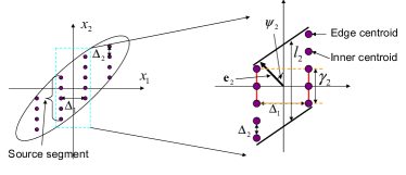
Figure 5: $x_{1},x_{2}$ plane of DQLC with $M=3$ when $\rho_{x}=0.95$. The expanded rectangle on the right can be applied to calculate anomalous errors for source $2$.

From Fig. 2 and 5 one can convince oneself that if $\Delta_{m}>2\alpha_{m+1}l_{m+1}/2$, the integrals in (28) can be avoided, since no distortion results from channel noise. For example, if $\Delta_{1}>2\alpha_{2}l_{2}/2$ in Fig. 2, the green stars will not be confused. One can derive from Fig. 5 that $l_{m+1}=2b_{m+1}\sqrt{\vartheta_{m+1}(1-\rho_{x})}$ (as was done for $l_{M}$ in section III-B). For large SNR, $\kappa_{m}$ become so large that one may neglect the $\ell_{\pm\kappa_{m}}[x_{m}]$ operation. The high-rate approximation to a scalar quantizer, $\Delta_{m}^{2}/12$, then applies to quantify distortion. To avoid constrained optimization, $D_{1}$ is further scaled by $P_{1}=MP-\sum_{i=2}^{M}P_{i}$. For convenience, we also scale $D_{m}$ by $P_{m}$ prior to quantization (instead of after). Note that when SNR gets large enough, $\kappa$ becomes so large and $\Delta_{m}$ becomes so small that $P_{m}\approx\alpha_{m}^{2}\sigma_{x}^{2}$.

The distortion at high SNR can be approximated by

$$\begin{split}&D_{1}\approx\frac{\alpha_{2}^{2}C_{2}(1-\rho_{x})}{3\bigg{(}MP-\sum_{i=2}^{M}\alpha_{i}^{2}\bigg{)}}\\ &D_{m}\approx\frac{\alpha_{m+1}^{2}C_{m+1}(1-\rho_{x})}{3\alpha_{m}^{2}},\hskip 2.84544ptm\in[2,M-2]\\ &D_{M-1}\approx\frac{\alpha_{M}^{2}C_{M}(1-\rho_{x})+(b_{n}\sigma_{n})^{2}}{3\alpha_{M-1}^{2}},\hskip 8.5359ptD_{M}\approx\frac{\sigma_{n}^{2}}{\alpha_{M}^{2}},\end{split}$$ (31)

where $C_{m}=b_{m}^{2}\vartheta_{m}^{2}$. For $D_{M}$, the high SNR approximation of (25) was used.

To determine the optimal performance, the optimal $\alpha_{m}^{2}$ needs to be found. The obvious way is to solve ${\nabla_{\overrightarrow{\alpha}}\big{[}D_{1}+D_{2}+\cdots+D_{M}\big{]}}=0$ with respect to $\alpha_{m}^{2}$. But since these are equations of order $\geq 4$, analytical solutions can not be found, and a different approach must be chosen. From the $M=2$ case in [3] is is known that the distortion of DQLC is a constant times the bound $\varrho_{2}$. We therefore hypothesize that this is the case for general $M$ as well: By choosing $\alpha_{M}^{2}=\sigma_{n}^{2}\mathcal{K}\varrho_{M}$, then $D_{M}=\mathcal{K}\varrho_{M}$. Since we want $D_{1}=D_{2}=\cdots=D_{M}=1/(\mathcal{K}\varrho_{M})$, the $\mathcal{K}$ that satisfies this relation must be determined. By solving $1/D_{M-1}=\mathcal{K}\varrho_{M}$, then

$$\begin{split}\alpha_{M-1}^{2}&=\frac{\sigma_{n}^{2}}{3}C_{M}(1-\rho_{x})\big{(}\mathcal{K}\varrho_{M}\big{)}^{2}\\ &=\frac{\alpha_{M}^{2}}{3}C_{M}(1-\rho_{x})\big{(}\mathcal{K}\varrho_{M}\big{)},\end{split}$$ (32)

assuming $b_{n}\sigma_{n}\approx 0$. By continuing to solve $1/D_{m}=\mathcal{K}\varrho_{M}$ with respect to $\alpha_{m}^{2}$ for $m$ from $M-2$ to $2$ using the previously derived $\alpha_{m+1}^{2}$, one can show that

$$\begin{split}\alpha_{i}^{2}&=\frac{\alpha_{M}^{2}}{3^{M-i}}\bigg{(}\prod_{j=i+1}^{M}C_{j}\bigg{)}(1-\rho_{x})^{M-i}\big{(}\mathcal{K}\varrho_{M}\big{)}^{M-i}.\end{split}$$ (33)

Finally, the $\mathcal{K}$ that makes $1/D_{1}=\mathcal{K}\varrho_{M}$, must be found. Expanding the sum $\sum_{i=2}^{M}\alpha_{i}^{2}$ using (33), and setting $C_{M+1}=1$, one can show that

$$\sum_{i=2}^{M}\alpha_{i}^{2}=\alpha_{M}^{2}\sum_{k=1}^{M-1}\bigg{(}\frac{(1-\rho_{x})\mathcal{K}\varrho_{M}}{3}\bigg{)}^{k-1}\prod_{j=M+2-k}^{M}C_{j}.$$ (34)

Letting $C_{2}=C_{3}=\cdots C_{M}=C$ (which is the case when $\rho_{ij}=\rho_{x},\forall i,j$ at high SNR), the product in (33) becomes $C^{-1}C^{k-1}$, and (34) turns into a Geometric series. From the sum of a Geometric series

$$\sum_{k=1}^{n}q^{k-1}=\frac{1-q^{n}}{1-q},$$ (35)

the following high SNR approximation can be derived

$$\sum_{i=2}^{M}\alpha_{i}^{2}\approx\frac{\alpha_{m}^{2}}{C}\bigg{(}\frac{(1-\rho_{x})C\mathcal{K}\varrho_{M}}{3}\bigg{)}^{M-2}.$$ (36)

Inserting (36) and (33) with $i=2$ into the expression for $D_{1}$ in (31)

$$\begin{split}&\bigg{(}M\text{SNR}-\frac{\alpha_{m}^{2}}{C}\bigg{(}\frac{(1-\rho_{x})C\mathcal{K}\varrho_{M}}{3}\bigg{)}^{M-2}\bigg{)}\cdots\\ &\bigg{(}\frac{(1-\rho_{x})C\mathcal{K}\varrho_{M}}{3}\bigg{)}^{1-M}=\mathcal{K}\varrho_{M},\end{split}$$ (37)

where SNR$=P/\sigma_{n}^{2}$. By solving (37) and removing constant terms, then

$$\mathcal{K}=\sqrt[M]{\bigg{(}\frac{3}{C}\bigg{)}^{M-1}}=\bigg{(}\frac{3}{C}\bigg{)}^{1-\frac{1}{M}},\hskip 7.11317pt\rho_{x}\neq 1.$$ (38)

(38) quantifies the loss to the performance upper bound. By inserting $C=b^{2}\vartheta$ and $M=2$ in (38), the loss calculated in [3] results, and so (38) is a generalization. One can observe that for any $M$ and $\rho_{x}$, DQLC exhibits a constant gap to the bound as SNR$\rightarrow\infty$. The gap grows somewhat with $M$, however, but is fortunately bounded: Taking the limit $M\rightarrow\infty$, the loss is $\approx 7.2$ dB when $\rho_{x}$ is close to 0 and $\approx 10.2$ dB when $\rho_{x}$ is close to 1. From (38) one can see that there are mainly two loss factors. One is due to short code length: When the code length is infinite, $b\rightarrow 1$ (see e.g. [17]), whereas when the code length is one, $b\approx 4$. The nested structure of DQLC results in an increased loss with $M$ whenever $b>1$. This accumulation is avoided with the S-K mappings described in Section II-C, as seen from Fig. 6. The distance to the upper bound is around 0.8-0.95 dB when $\rho_{x}=0$, actually decreasing slightly when $M$ increases (the same effect is observed when $\rho_{x}$ is close to 1, but the loss is now around 2 dB). This clearly indicates that it is not the zero delay requirement alone that makes the loss increase with $M$. The reason for the increasing loss is most likely that the DQLC is sub-optimal. Alternatively, it may be that zero delay distributed JSCC schemes will suffer from an increasing loss like (38). This must be dismissed or confirmed through further research, however. The reason why $\vartheta=2$ when $\rho_{x}$ is close to one is that the source space can not be rotated (decorrelation) with the choice of distributed encoders, and this implies that each channel segment gets somewhat longer than necessary.

By inserting $b\approx 4$ and $\vartheta\approx 1$ when $\rho_{x}$ is close to zero, and $\vartheta\approx 2$ when $\rho_{x}$ is close to 1, the performance of DQLC as a function of $M$ can be plotted. Fig. 6 shows the loss from upper bound for DQLC (high SNR in general) and uncoded transmission at 100 dB SNR. S-K mappings for $\rho_{x}=0$ case is also shown (results are taken from [11, chapter 3] and [18]).

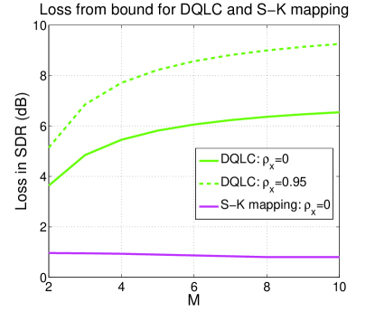
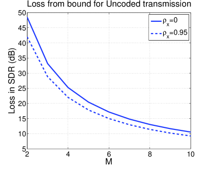
Figure 6: Loss in SDR from upper bound at SNR$=100$ dB. (a) DQLC. (b) Uncoded transmission.

From these plots one can see that the performance of uncoded transmission will close in on the performance of DQLC when around 10 sources are considered. This number will decrease somewhat for smaller SNR and increase as the SNR gets higher. Note that for uncoded transmission the distance to the bound will in any case increase as the SNR grows (except when $\rho_{x}=1$), contrary to DQLC, and so DQLC will improve over uncoded transmission when the SNR gets sufficiently large, thus fulfilling our objective.

IV Optimization and simulation of DQLC at arbitrary SNR when $M=3$

We give an example on how to calculate and optimize distortion for all SNR when $M=3$ by applying the analysis in Section III-C. The optimized DQLC is further simulated and compared to distortion lower bound, S-K mapping and uncoded transmission.

IV-A Calculation of distortion

The distortion for source $3$ is found from Section III-C by setting $M=3$ in (21), (24) and (25), and the channel power is given by (26). Furthermore, the distortion from quantization and limitation of source $1$ and $2$ is given by (27) and the power is given by (29). What remains to calculate is the distortion due to channel noise for source $1$ and $2$ given by (28). When analyzing DQLC around its optimal distortion, only jumps to the nearest neighboring centroids needs to be considered. This will simplify the calculations and speed up the optimization process. As for source 3,  (28) can be divided into channel- and anomalous distortion. As mentioned in Section  III-C2, both channel distortion and anomalous distortion may occur for source 2, while only channel distortion may occur for source 1.

Anomalous distortion for source 2: A similar analysis to that in Section III-C1 applies here. As for anomalous distortion for source 3, there are two cases to consider: $l_{2}>2\kappa_{2}$ and $l_{2}\leq 2\kappa_{2}$. Now $l_{2}=b_{2}\sigma_{x}\sqrt{2(1-\rho_{x})}$ and calculated in the same way as $l_{M}$ in Section III-B, now using the parallelogram to the right in Fig. 5. $b_{2}$ is a constant that determines the width of the ellipse (in Fig. 5) containing the significant (quantized) probability mass.

Assume first that $l_{2}>2\kappa_{2}$ (see $\rho_{x}=0$ case in Fig. 2). The error we get when anomalies start to happen is the difference in magnitude between centroid no. 1 and centroid no. $N_{q_{2}}$, i.e. $|q_{({N_{q_{2}}})_{2}}-q_{1_{2}}|=\Delta_{2}(N_{q_{2}}-1)$. The probability for anomalies (the probability for crossing of the decision borders for encoder 1 in Fig. 2) is given by

$$p_{th2}=Pr\{|f_{2}(x_{2})+f_{3}(x_{3})+n|\geq d_{1}/2\}=P_{N_{q_{2}}}p_{d_{th}},$$ (39)

where $P_{N_{q_{2}}}=Pr\{(N_{q_{2}}-1)\Delta_{2}/2<x_{2}<\infty\}$ is the probability for being at an edge centroid (see Fig. 2) and $p_{d_{th}}=Pr\{|y_{3}+n|>d_{th}\}$, where

$$d_{th}=\frac{d_{1}}{2}-\frac{\alpha_{2}d_{2}}{2}(N_{q_{2}}-1),$$ (40)

is the distance from an edge centroid of encoder 2 to the decision border of encoder 1 (see Fig. 2). The distribution needed to calculate $p_{d_{th}}$ is given in (17).

Now consider the case $l_{2}\leq 2\kappa_{2}$ ($\rho_{x}=0.95$ scenario in Fig. 2). This case is difficult to calculate as accurately as the $l_{2}>2\kappa_{2}$ case above, since its hard to determine exactly which centroids that are edge centroids (this can be seen by comparing the $\rho_{x}=0.95$ case with the $\rho_{x}=0$ case in Fig. 2). One can get around this problem by calculating both the probability $\tilde{p}_{th2}=Pr\{|f_{2}(x_{2})+f_{3}(x_{3})+n|\geq d_{1}/2\}$ and the resulting anomalous error assuming that $y_{2}=f_{2}(x_{2})$ is continuous. By using $p_{z_{M}(\overrightarrow{i}_{m})}(z_{M})_{\gamma_{M}}$ in (19) and the expression for $p(y_{2}|x_{1})$ (see [13, p.223]) one can show that

$$\begin{split}&\tilde{p}_{th2}=\int_{d_{1}/2}^{\infty}\big{[}p_{z_{M}(\overrightarrow{i}_{m})}(z_{M})_{\gamma_{M}}\ast p(y_{2}|x_{1})\big{]}(z)\mbox{d}z\\ &=\int_{d_{1}/2}^{\infty}\frac{e^{-\frac{1}{2}\frac{(\mu-z_{M})^{2}}{\sigma_{n}^{2}+\Sigma_{aa\cdot b}+\sigma_{x}^{2}\alpha_{2}^{2}(1-\rho_{x}^{2})}}}{\sqrt{2\pi\big{(}\sigma_{n}^{2}+\Sigma_{aa\cdot b}+\sigma_{x}\alpha_{2}\sqrt{2\pi(1-\rho_{x}^{2})}\big{)}}}\mbox{d}z,\end{split}$$ (41)

where $d_{1}=\Delta_{1}\big{(}1+\rho_{x}(\alpha_{2}+\alpha_{3})\big{)}$. As in Section III-C1, the probability in (41) is calculated assuming $\mu=0$. With the same reasoning as in Section III-C1, one can show that the error we get when anomalies start to happen is approximately $\gamma_{2}=l_{2}-\Delta_{1}=b_{2}\sigma_{x}\sqrt{2(1-\rho_{x})}-\Delta_{1}$ (see Fig. 5).

The anomalous distortion becomes

$$\bar{\varepsilon}_{an2}^{2}=\begin{cases}p_{th2}\big{(}\Delta_{2}(N_{q_{2}}-1)\big{)}^{2},&l_{2}>2\kappa_{2},\vspace{0.3cm}\\ \tilde{p}_{th2}\gamma_{2}^{2},&l_{2}\leq 2\kappa_{2},\end{cases}$$ (42)

where $2\kappa_{2}=\Delta_{2}(N_{q_{2}}-1)$.

Channel distortion, source 2: Since anomalous errors results for source 3 whenever channel errors occur for source 2, the validity for these events are the same. A similar expression to that in (42) can therefore be derived:

Consider first $l_{3}>2\kappa_{3}$: For a given source segment in the $x_{1},x_{2}$ plane an inner centroid has two neighbors, while an edge centroid has only one (see Fig. 5). The probability that an inner centroid is confused with its neighbors is given by $p_{th3}$, found by substituting $M=3$ in (22). For edge centroids we have $p_{th3}/2$ since channel errors happens if an edge centroid is exchanged with an inner centroid, whereas anomalous errors happen otherwise (see Fig. 2). When neighboring centroids are exchanged, the error is $\Delta_{2}^{2}$. With $P_{N_{q_{2}}}$, the probability for an edge centroid, then

$$\begin{split}\bar{\varepsilon}_{C_{2}}^{2}&=2\Delta_{2}^{2}p_{th_{3}}\sum_{i=2}^{\frac{N_{q_{2}}}{2}}P_{i}+\Delta_{2}^{2}2P_{N_{q_{2}}}\frac{p_{th_{3}}}{2}\\ &=2\Delta_{2}^{2}p_{th_{3}}\big{(}1/2-P_{N_{q_{2}}}\big{)}+\Delta_{2}^{2}P_{N_{q_{2}}}p_{th_{3}}\\ &=\Delta_{2}^{2}p_{th_{3}}\big{(}1-P_{N_{q_{2}}}\big{)}.\end{split}$$ (43)

Now assume $l_{3}\leq 2\kappa_{3}$: As for anomalous distortion, this case is difficult to calculate accurately, due to the difficulty of determining which centroids are edge centroids. One can, however, upper bound channel distortion by assuming that jumps from any centroid leads to channel distortion (i.e. none of the possible events leads to anomalous distortion). The probability for channel distortion is then given by $\tilde{p}_{th3}$, found by substituting $M=3$ in (23). We therefore have $\bar{\varepsilon}_{C_{2}}^{2}\leq\Delta_{2}^{2}\tilde{p}_{th_{3}}$. This bound is accurate enough to find the optimal parameters of DQLC.

Channel distortion, source 1: Since $N_{q_{1}}=\infty$ and no threshold effects happen for source 1, the probability for channel distortion for source 1 will be the same as the probability for threshold effects for source 2. The magnitude of the error is $\Delta_{1}^{2}$. Therefore $\bar{\varepsilon}_{C_{1}}^{2}=\Delta_{1}^{2}p_{th_{2}}$ when $l_{2}>2\kappa_{2}$, and $\bar{\varepsilon}_{C_{1}}^{2}=\Delta_{1}^{2}\tilde{p}_{th_{2}}$ when $l_{2}\leq 2\kappa_{2}$.

IV-B Optimization and Simulation

Instead of solving the constrained problem in (15), we choose to scale $x_{1}$ by $\xi=\sqrt{3P-(P_{2}(\Delta_{2},\alpha_{2})+P_{3}(\alpha_{3},\kappa_{3}))}/\sigma_{x}$ prior to quantization to get an unconstrained problem. Note that the factor $q_{i_{m}}(1+\rho_{x}(\alpha_{2}+\alpha_{3}))$ in (12) must then be changed to $q_{i_{m}}(1+\rho_{x}(\alpha_{2}+\alpha_{3})/\xi)$ in order to decode correctly (the integration limit in (41) must also be changed). The average distortion for DQLC is $D=(D_{1}+D_{2}+D_{3})/3$, where

$$\begin{split}D_{1}&=\frac{\bar{\varepsilon}_{q,1}^{2}(\Delta_{1})+\bar{\varepsilon}_{C_{1}}^{2}(\Delta_{1},\alpha_{2},N_{q_{2}})}{\xi(\Delta_{2},\alpha_{2},\alpha_{3},\kappa_{3})},\\ D_{2}&=\bar{\varepsilon}_{q,2}^{2}(\Delta_{2},N_{q_{2}})+\bar{\varepsilon}_{C_{2}}^{2}(\Delta_{2},N_{q_{2}},\alpha_{2},\alpha_{3},\kappa_{3})\\ &+\bar{\varepsilon}_{an2}^{2}(\Delta_{2},N_{q_{2}},\alpha_{2},\alpha_{3},\kappa_{3}),\\ D_{3}&=\bar{\varepsilon}_{\kappa_{3}}^{2}(\kappa_{3})+\bar{\varepsilon}_{C_{3}}^{2}(\alpha_{3},\beta)+\bar{\varepsilon}_{an3}^{2}(\Delta_{2},\alpha_{2},\alpha_{3},\kappa_{3}).\end{split}$$ (44)

All parameters must be greater than zero and $\alpha_{2}\geq\alpha_{3}$. Some of the distortion terms do not have analytical solutions, and thus numerical optimization is necessary to determine the optimal parameters.

DQLC is compared to the bound from Section II-B, uncoded transmission from Section II-D and the S-K mappings from Section II-C. Again we choose to look at signal-to-distortion ratio (SDR) $\sigma_{x}^{2}/D$ as a function of channel SNR $=P/\sigma_{n}^{2}$ (and $\rho_{x}$) instead of distortion. The results are shown in Fig. 7 for $\rho_{x}=0$ and $\rho_{x}=0.95$.

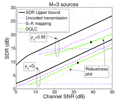
Figure 7: Performance of DQLC compared to the SDR upper bound, S-K mappings and uncoded transmission. The black dots shows the design SNR for the robustness plots for DQLC.

The SDR upper bound is given by $\sigma_{x}^{2}/D^{*}$, where $D^{*}$ is the optimal distortion given in (3).

When $\rho_{x}=0$, DQLC drops around 2.5-3.5dB from the upper bound, while it drops around 4 to 7 dB when $\rho_{x}=0.95$. The loss at high SNR (50dB) corresponds well with the calculated estimate shown in Fig. 6 when $\rho_{x}=0.95$, while the calculated estimate is a bit pessimistic when $\rho_{x}=0$. Fortunately, DQLC gets somewhat closer to the bound as the SNR drops. There is also a backoff to the S-K mapping of around 1 to 2 dB. This is because S-K mappings avoid threshold effects as well as the “loss accumulation” mentioned in Section III-D. Interestingly, DQLC improves with increasing $\rho_{x}$ without changing the basic encoder and decoder structure, only the different parameters needs to be adapted. The improvement is significant, around 5 to 7 dB when $\rho_{x}$ goes from 0 to 0.95. DQLC is also robust against variations in noise level. Note that DQLC outperform uncoded transmission for SNR$>7$dB when $\rho_{x}=0$ and SNR$>28$dB when $\rho_{x}=0.95$.

The gain from increasing correlation as a function of $\rho_{x}$ is shown in Fig. 8 for DQLC and uncoded transmission at 40 dB channel SNR.

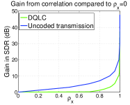
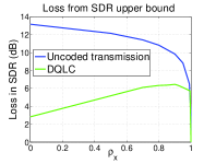
Figure 8: How correlation affects performance when $M=3$ at 40 dB channel SNR. (a) Gain from correlation for DQLC and uncoded transmission. (b) Loss from SDR upper bound as a function of $\rho_{x}$.

Note that the gain for DQLC is not significant before $\rho_{x}>\approx 0.7$, whereas the gain gets large when $\rho_{x}\rightarrow 1$ (around 37.5 dB). Uncoded transmission shows an even greater gain, which is natural since it goes from being highly sub-optimal when $\rho_{x}=0$ to achieve the bound for all SNR when $\rho_{x}=1$. The gap to the performance upper bound as a function of $\rho_{x}$ is plotted for DQLC and uncoded transmission in Fig. 8, for 40dB channel SNR. Note that the distance to the upper bound is largest for DQLC when $\rho_{x}$ is around $0.9$, and that DQLC and uncoded transmission both reach the upper bound in the limit $\rho_{x}\rightarrow 1$. Note that DQLC performs better than uncoded transmission for most $\rho_{x}$ values at 40dB SNR.

If there is a demand for equal transmit power from each encoder, one can still use DQLC with timesharing. I.e. each encoder described here is used on each source 1/3 of the time (1/M in general). As shown for the $M=2$ case in [3], a further backoff from the bound compared to that in Fig. 7 must then be expected.

V Summary and extensions

In this paper, a distributed delay-free and low complexity joint source-to-channel mapping was proposed and bounds were derived for transmission of a multivariate Gaussian over a Gaussian MAC. Both linear and nonlinear mappings were analyzed. A linear mapping (uncoded transmission) achieves the performance upper bound within a certain range of low channel SNR. A nonlinear mapping, DQLC, was introduced to improve on uncoded transmission at higher SNR. A collaborative scheme (Shannon-Kotel’nikov mapping) was also introduced to provide an approximate bound for zero delay schemes.

DQLC does not achieve the performance upper bound, but leaves a certain gap which value depends on both correlation and the number of sources. However, DQLC constitutes a constant gap to the bound in any case as SNR$\rightarrow\infty$ and its received fidelity (SDR) improves with increasing correlation without changing the basic encoder and decoder structure. DQLC therefore outperforms uncoded transmission as the SNR gets high enough in any case. Unfortunately, the loss to the bound increases somewhat with the number of sources (something the collaborative S-K mappings does not), but is fortunately bounded to a finite value as the number of sources goes to infinity. Optimization and simulation for 3 sources also showed that the gap to the bound decreases somewhat as the SNR drops.

It is also important to note that DQLC can be applied for any unimodal source (and channel) distribution and optimized using the same method as presented in this paper.

Future research should aim at finding, if possible, a scheme where the loss to the bound does not increase with the number of sources, as is the case for the collaborative S-K mappings. The generalization of DQLC to arbitrary code length should also be investigated. Recently it has been shown that such a generalization achieves the performance upper bound when SNR is high for any number of uncorrelated sources [17]. What remains is to prove what happens for arbitrary correlation and SNR. The impact of practical issues like imperfect timing and synchronization should also be addressed in order to get a step closer to a possible practical realization.

References

- [1] M. Gastpar, “Uncoded transmission is exactly optimal for a simple Gaussian “sensor” network,” IEEE Trans. Information Theory, vol. 54, no. 11, pp. 5247–5251, Nov. 2008.
- [2] A. Lapidoth and S. Tinguely, “Sending a bivariate Gaussian over a Gaussian MAC,” IEEE Trans. Information Theory, vol. 56, no. 6, pp. 2714–2752, Jun. 2010.
- [3] P. A. Floor, A. N. Kim, N. Wernersson, T. Ramstad, M. Skoglund, and I. Balasingham, “Zero-delay joint source-channel coding for a bivariate Gaussian on a Gaussian MAC,” IEEE Trans. Commun., vol. 60, no. 10, Oct. 2012.
- [4] P. A. Floor, A. N. Kim, T. A. Ramstad, I. Balasingham, N. Wernersson, and M. Skoglund, “Transmitting multiple Gaussian sources over a Gaussian MAC using delay-free mappings,” in 4th International Symposium on Applied Sciences in Biomedical and Communication Technologies (ISABEL). Barcelona, Spain: ACM, Oct. 2011.
- [5] T. M. Cover and J. A. Thomas, Elements of Information Theory. New York: Wiley, 2006.
- [6] T. A. Ramstad, “Shannon mappings for robust communication,” Telektronikk, vol. 98, no. 1, pp. 114–128, 2002. [Online]. Available: http://www.telenor.com/telektronikk/volumes/pdf/1.2002/Page_114-128.pdf
- [7] F. Hekland, P. A. Floor, and T. A. Ramstad, “Shannon-Kotel’nikov mappings in joint source-channel coding,” IEEE Trans. Commun., vol. 57, no. 1, pp. 94–105, Jan. 2009.
- [8] P. A. Floor and T. Ramstad, “Shannon-Kotel’nikov mappings for analog point-to-point communications.” arXiv:1101.5716v2 [cs.IT], 2012.
- [9] E. Akyol, K. Rose, and T. A. Ramstad, “Optimal mappings for joint source channel coding,” in Proc. Information Theory Workshop (ITW). Dublin, Ireland: IEEE, Aug. 30th - Sept. 3rd 2010.
- [10] Y. Hu, J. Garcia-Frias, and M. Lamarca, “Analog joint source-channel coding using non-linear curves and mmse decoding,” IEEE Trans. Commun., vol. 59, no. 11, pp. 3016–3026, Nov. 2011.
- [11] A. Fuldseth and T. A. Ramstad, “Bandwidth compression for continuous amplitude channels based on vector approximation to a continuous subset of the source signal space,” in Proc. IEEE Int. Conf. on Acoustics, Speech, and Signal Proc. (ICASSP), 1997.
- [12] A. Fuldseth, “Robust subband video compression for noisy channels with multilevel signaling,” Ph.D. dissertation, Norwegian University of Science and Engineering (NTNU), 1997.
- [13] A. Papoulis and S. U. Pillai, Probability, Random Variables and Stochastic Processes, 4th ed. New York: McGraw-Hill higher education, Inc, 2002.
- [14] C. E. Shannon, “Communication in the presence of noise,” Proc. IRE, vol. 37, pp. 10–21, Jan. 1949.
- [15] N. Merhav, “Threshold effects in parameter estimation as phase transitions in statistical mechanics,” IEEE Trans. Information Theory, vol. 57, no. 10, pp. 7000–7010, Oct. 2011.
- [16] J. M. Wozencraft and I. M. Jacobs, Principles of Communication Engineering. New York: John Wiley & Sons, Inc, 1965.
- [17] P. A. Floor, A. N. Kim, T. A. Ramstad, and Balasingham, “On transmission of multiple Gaussian sources over a Gaussian MAC using a VQLC mapping,” in Information Theory Workshop (ITW). Lausanne, Switzerland: IEEE, Sept. 3rd-7th 2012.
- [18] P. A. Floor, “On the theory of Shannon-Kotel’nikov mappings in joint source-channel coding,” Ph.D. dissertation, Norwegian University of Science and Engineering (NTNU), 2008.
- [19] R. J. Muirhead, Aspects of Multivariate Statistical Theory. John Wiley & Sons, Inc., Publicator, 1982.