A slave mode expansion for obtaining ab-initio interatomic potentials

Abstract

Here we propose a new approach for performing a Taylor series expansion of the first-principles computed energy of a crystal as a function of the nuclear displacements. We enlarge the dimensionality of the existing displacement space and form new variables (ie. slave modes) which transform like irreducible representations of the space group and satisfy homogeneity of free space. Standard group theoretical techniques can then be applied to deduce the non-zero expansion coefficients a priori. At a given order, the translation group can be used to contract the products and eliminate terms which are not linearly independent, resulting in a final set of slave mode products. While the expansion coefficients can be computed in a variety of ways, we demonstrate that finite difference is effective up to fourth order. We demonstrate the power of the method in the strongly anharmonic system PbTe. All anharmonic terms within an octahedron are computed up to fourth order. A proper unitary transformation demonstrates that the vast majority of the anharmonicity can be attributed to just two terms, indicating that a minimal model of phonon interactions is achievable. The ability to straightforwardly generate polynomial potentials will allow precise simulations at length and time scales which were previously unrealizable.

I Introduction

While the first-principles computation of the harmonic vibrational properties of crystals with sufficient symmetry is ubiquitousBaroni et al. (2001); Kunc and Martin (1982); Alfe (2009); Parlinski et al. (1997); VandeWalle and Ceder (2002), the same cannot be said for the anharmonic counterparts. The reasons for this are somewhat indirect. Density functional theory (DFT), within the Born-Oppenheimer approximation, can accurately predict the forces and stresses in many classes of materials and therefore could be used to compute both quantum and classical dynamics of the nuclei. However, the scaling of DFT severely restricts the applicability of such a task to very short timescales and small unit cells. Generically, there are a number of different approaches to overcoming this fundamental limitation which exchange accuracy for efficiency, including fully empirical approaches which replace DFT, semi-empirical electronic structure approachesPapaconstantopoulos and Mehl (2003), and linear scaling DFTBowler and Miyazaki (2012); Vandevondele et al. (2012).

One obvious approach which has a long history is to perform a Taylor series expansion of the energy as a function of the nuclear displacements, allowing for extremely high precision up to some order and within some range. While such an approach will have obvious limitation (ie. large deformations, diffusion, etc.), it has a negligible computational cost relative to DFT, allowing length and timescales which could not even be considered within DFT. Furthermore, it has additional appeal in that the expansion coefficients are basic materials properties. Understanding the anharmonic interactions across a broad range of materials will help understand a myriad of materials properties in terms of a low energy model. While the number of anharmonic terms rapidly increases with the order of the expansion, we demonstrate in this work that there is reason to be optimistic that a minimal number of expansion coefficients can capture the bulk of the physics. While the Hubbard and Anderson models have guided us for many years in terms of understanding electronic phenomena in transition metal oxides and actinide based materialsKotliar et al. (2006), analogues are clearly needed in the context of the interacting phonon problem.

Some of the early executions of an anharmonic Taylor series expansion based on first-principles calculations where executed by Vanderbilt et al in the context of SiVanderbilt et al. (1989) and by Rabe and Vanderbilt et al. in the context of ferroelectric materialsKingsmith and Vanderbilt (1994); Zhong et al. (1994, 1995). These approaches were quite successful, correctly capturing the proper ordering of different phases as a function of temperature and even providing quantitatively accurate transition temperatures. In terms of the expansion, a variety of different philosophies were taken in these works. The earliest of these works which focussed on SiVanderbilt et al. (1989) employed a quartic expansion in terms of bond bending and stretching variables in the spirit of earlier work of KeatingKeating (1966a, b). Coupling to strain becomes critical in the ferroelectric materials, and an expansion similar to that of PyttePytte (1972) was used by Vanderbilt et alKingsmith and Vanderbilt (1994) to encode the properties of various perovskites. Subsequent work by Rabe et alZhong et al. (1994, 1995) utilized a novel lattice Wannier function approachRabe and Waghmare (1995) to perform an anharmonic expansion (see refIniguez et al. (2000) for a related approach).

With the continued explosion of computational resources, more recent works have revisited this problem. Esfarjani and Stokes considered the generic Taylor series expansion and all the symmetry constraints that the expansion must satisfyEsfarjani and Stokes (2008). They then generated a large data set from first-principles calculations and fit the expansion parameters to the data under the symmetry constraints. A number of materials and phenomena have been studied using this approach, including the thermal conductivity in Si, half-Heusler compounds, and PbTeEsfarjani et al. (2011); Shiomi et al. (2011); Shiga et al. (2012). Wojdel et al.Wojdel et al. (2013) employed a different approach, expanding in displacement differences between pairs of nuclei, similar in spirit to early model calculationsKeating (1966a, b), and they included point symmetry by projecting displacement difference polynomials onto the identity representation. Additionally, Wojdel et al. explicity consider strain degrees of freedom and their coupling to local displacements, similar to earlier works in ferroelectric materials.

It is also worth mentioning recent machine learning approaches that have the potential to have significant impact in this space. Behler and Parrinello used a neural-network to parameterize the DFT energyBehler and Parrinello (2007), and they have achieved impressive results on NaEshet et al. (2010, 2012) and graphite/diamondKhaliullin et al. (2011). These results suggest that appropriate neural-networks have the potential to accurately describe structural phase transitions in a broad range of systems, though it is still unclear if they have sufficient resolution to accurately capture phonons and higher derivatives of the energy. Another approach in the context of machine learning is so-called compressive sensing, which has been applied in the context of alloy theory to parameterize cluster expansionsNelson et al. (2013) and has also shown promise in the context of lattice dynamics.

Despite the great successes of the aformentioned expansions, they have not yet become ubiquitous, perhaps because it is nontrivial to execute the parameterization. Here we introduce a new approach which combines many of the advantages of the different methods discussed above. Our approach allows us to circumvent the difficulties of fitting data across multiple orders, builds in all the necessary symmetry from the beginning, is generally applicable, provides a convenient notation to encode our parameters such that others may use them, and in the case of PbTe we show that a physically motivated unitary transformation can compress hundreds of anharmonic terms into just two.

II Method

II.1 Background

We will start by considering the total energy of a crystal assuming that the Born-Oppenheimer approximation is valid. The Taylor series expansion of the total energy as a function of the nuclear displacements can be written as followsEsfarjani and Stokes (2008):

$$V =\sum_{\alpha\beta\mathbf{R}_{a}\mathbf{R}_{b}}\Psi(\mathbf{R}_{a},\mathbf{R}_{b})_{\alpha\beta}u^{\mathbf{R}_{a}}_{\alpha}u^{\mathbf{R}_{b}}_{\beta}$$ (1)

$$+\sum_{\alpha\beta\gamma\mathbf{R}_{a}\mathbf{R}_{b}\mathbf{R}_{c}}\Psi(\mathbf{R}_{a},\mathbf{R}_{b},\mathbf{R}_{c})_{\alpha\beta\gamma}u^{\mathbf{R}_{a}}_{\alpha}u^{\mathbf{R}_{b}}_{\beta}u^{\mathbf{R}_{c}}_{\gamma}$$

$$+\sum_{\begin{subarray}{c}\alpha\beta\gamma\delta\\ \mathbf{R}_{a}\mathbf{R}_{b}\mathbf{R}_{c}\mathbf{R}_{d}\end{subarray}}\Psi(\mathbf{R}_{a},\mathbf{R}_{b},\mathbf{R}_{c},\mathbf{R}_{d})_{\alpha\beta\gamma\delta}u^{\mathbf{R}_{a}}_{\alpha}u^{\mathbf{R}_{b}}_{\beta}u^{\mathbf{R}_{c}}_{\gamma}u^{\mathbf{R}_{d}}_{\delta}$$

$$+\cdots$$

Where $\Psi$ are the direct expansion coefficients, $u$ are the nuclear displacements, $\mathbf{R}=n_{1}\mathbf{v}_{1}+n_{2}\mathbf{v}_{2}+n_{3}\mathbf{v}_{3}$ ($n_{i}$ are integers, $\mathbf{v}_{i}$ are unit cell vectors), $\alpha,\beta,\gamma,\delta$ label both the displacement direction (ie. $x,y,z$) and the atom within the unit cell. The number of terms dramatically increases as the order increases. Therefore, a condition for this expansion to be useful is locality: the expansion coefficients must decay sufficiently rapidly in some representation for terms beyond quadratic order. This cannot be known a priori and only explicit testing could determine the viability of this approach. Symmetry will be crucial both to reduce the number of terms at a given order and to ensure that the expansion is robust for use in simulations. The following symmetries must be satisfied:

1. The energy must be invariant to all space group operations.

2. Homogeneity of free space with respect to rigid translation. If the entire crystal is shifted by an arbitrary constant, there cannot be any change in the total energy nor its derivatives.

3. Homogeneity of free space with respect to rigid rotation. If the entire crystal is rotated about some point by an arbitrary amount, there cannot be any change in the total energy nor its derivatives.

4. If the energy function is analytic, the derivatives will be invariant of the order in which they are taken.

These symmetries result in a series of constraints on the expansion coefficientsEsfarjani and Stokes (2008). The central task at hand is to actually compute the derivatives of the energy with respect to the atomic displacements and ensure that they satisfy all of the symmetries.

II.2 Slave Mode Expansion

Executing the expansion would be far more straightforward if the symmetry could be somehow imposed from the beginning. This can be achieved at the expense of enlarging the dimensionality of the system. Instead of using nuclear displacement parameters $u$, we will introduce so-called slave modes $\phi$ which transform like irreducible representations of the space group and satisfy homogeneity of free-space. These slave modes may then be used to expand the potential, and all of the symmetry constraints will be built into the expansion. Enlarging the dimensionality does come at an expense, as some of the slave mode products will be linearly dependent, but this can be handled in a straightforward fashion. It should be noted that the one symmetry we do not consider is homogeneity of free space with respect to rotations, which will link coefficients at different ordersEsfarjani and Stokes (2008). Fortunately, any associated errors will not accumulate due to the satisfaction of point group symmetry. We now expand the energy in terms of the slave modes:

$$V =\sum_{\mathbf{R}s}\sum_{\alpha i}\Phi_{\alpha}^{s}\hskip 2.84526pt\phi_{\alpha\mathbf{R}s}^{(i)}\phi_{\alpha\mathbf{R}s}^{(i)}$$ (2)

$$+\sum_{\mathbf{R}s}\sum_{\begin{subarray}{c}\alpha\beta\gamma\\ \xi,ijk\end{subarray}}\Phi_{\alpha\beta\gamma}^{s\xi}\Theta_{\alpha\beta\gamma}^{\xi,ijk}\hskip 2.84526pt\phi_{\alpha\mathbf{R}s}^{(i)}\phi_{\beta\mathbf{R}s}^{(j)}\phi_{\gamma\mathbf{R}s}^{(k)}$$

$$+\sum_{\mathbf{R}s}\sum_{\begin{subarray}{c}\alpha\beta\gamma\delta\\ \xi,ijkl\end{subarray}}\Phi_{\alpha\beta\gamma\delta}^{s\xi}\Theta_{\alpha\beta\gamma\delta}^{\xi,ijkl}\hskip 2.84526pt\phi^{(i)}_{\alpha\mathbf{R}s}\phi^{(j)}_{\beta\mathbf{R}s}\phi^{(k)}_{\gamma\mathbf{R}s}\phi^{(l)}_{\delta\mathbf{R}s}+\cdots$$

where $\alpha,\beta,\gamma,\delta$ label irreducible representations, $i,j,k,l$ label rows of a given irreducible representation, $\xi$ labels a given identity representation within the product representation, $\mathbf{R}$ is a lattice vector, $s$ labels a cluster within the unit cell, $\Theta$ are the Clebsch-Gordan (CG) coefficients, $\Phi$ are the irreducible expansion coefficients, and $\phi$ are the slave modes. It should be noted that cross terms between the clusters with different $\mathbf{R}$ or $s$ are not written as their contribution can be accounted for by simply including larger clusters. The CG coefficients are a group theoretical construct which are independent of any particular application, and these may be straightforwardly computed. However, care must be taken to ensure that a consistent phase convention has been used as there is no unique definition. The slave clusters $\phi$ are a linear combination of atomic displacements which transform like the irreducible representation of a given point group in the crystal. While we have explicitly written out the quadratic terms, we will assume that these will normally be obtained using traditional approaches to compute phonons.

There is a wide degree of flexibility in choosing the slave modes, and the optimum choice may depend on the material and the use of the method. Here we will outline a typical scenario, and specific cases will be dealt with later in the manuscript.

1. Determine a cluster of atoms for which the anharmonic terms will be included. This cluster will be associated with a given unit cell (typically primitive), though it could contain atoms which are outside of the unit cell. As the size of the cluster increases, the number of terms in the expansion will increase markedly, so this choice must be made judiciously. At least two atoms must be present in this cluster. We will refer to this as the slave cluster.

2. A center of highest symmetry should be identified for the chosen cluster and the associated point group should be determined. Each atom in the cluster will have $d$ degrees of freedom, where $d$ is the dimension of space. The displacement vectors should then be projected onto the irreducible representation of the point group.

3. $d$ of the irreducible representations that correspond to a uniform shift of the cluster need to be eliminated as they would violate homogeneity of free space. The remaining modes are the slave modes, and they can essentially be thought of as molecular entities. The usual methods of finite group theory may be used to show that only products transforming like the identity are non-zeroCornwell (1997); Tinkham (1964).

4. All non-translation space group operations should be used to determine if translationally inequivalent slave clusters are generated from the initial set.

5. The translation group may then be used to generate all translationally equivalent sets.

It may be useful to have multiple types of slave clusters associated with each unit cell, and then the above procedure will be executed for each slave cluster. This will indeed be the case for PbTe.

At this point, one has an expansion which respects all of the necessary symmetries, albeit at the expense of increasing the dimensionality of the system. If one began with a crystal having $\alpha$ atoms per unit cell in $d$ dimensions and there are $N$ unit cells in the crystal, then the total number of degrees of freedom would be $(N\alpha-1)d$. If one chose a single cluster per unit cell having $z$ atoms, then the total number of degrees of freedom would be $(z-1)dN$. Under normal conditions $z>2$, and therefore the dimensionality of the system has increased. This does give rise to several issues. First, if one wanted to use the slave modes as independent variables, then a constraint would have to be satisfied in order to be sure that the vibrational state is physical. In other words, an arbitrary vector in the space of slave modes will not necessarily have a corresponding vector in the space of displacements. However, this poses no problem in this work as we will always be using the slave modes as dependent variables. The second issue is that slave mode products at a given order which are irreducible with respect to point symmetry will not necessarily be linearly independent when lattice translations are included, and therefore certain mode products must be eliminated to remove linear dependency. This is a penalty that must be dealt with in order to take this approach. A final point worth noting is that slave modes on different sites are not orthogonal as we have presented them in this work. This means that an amplitude for a slave mode on one-site will induce a non-zero amplitude on its neighbor. However, this poses no real challenges to the method.

II.3 Slave mode Expansion for the $2d$ Square Lattice

To illustrate the slave mode expansion we apply it to a two dimensional square lattice with one atom in one unit cell. We will explore two difference choices for slave modes. First, let us consider a cluster of two nearest-neighbor atoms (ie. dimer cluster). In this case, we will choose the center of the cluster as the midpoint of the bond (see figure 1 top panel), which will have point group $C_{2v}$. The $C_{2v}$ point group allows four different irreducible representations, and we follow the usual convention of $A_{1},A_{2},B_{1},B_{2}$Cornwell (1997). The representation for the dimer cluster is four dimensional and can be decomposed as $\Gamma=A_{1}\oplus A_{2}\oplus B_{1}\oplus B_{2}$ (see figure 1 top panel). The two normal modes $B_{1}\oplus B_{2}$ correspond to uniform shifts of the cluster, and therefore these modes will be removed, as indicated by the red $X$, leaving only $A_{1}\oplus A_{2}$. Using the Great Orthogonality Theorem (GOT)Cornwell (1997); Tinkham (1964), one can deduce that only the products that transform like the identity will be nonzero, and these can be determined by inspecting the character table of $C_{2v}$. There will be two slave mode products at second order: $\phi_{A_{1}}^{2}$ and $\phi_{A_{2}}^{2}$. At third order there will be two terms: $\phi_{A_{1}}^{3}$ and $\phi_{A_{2}}^{2}\phi_{A_{1}}$. At fourth order there will be three terms: $\phi_{A_{1}}^{4}$, $\phi_{A_{2}}^{4}$, and $\phi_{A_{2}}^{2}\phi_{A_{1}}^{2}$. One can easily proceed to higher orders, but we will remain at quadratic order for the sake of simplicity in this example. At this point, one needs to see if any non-translational symmetry elements will generate a new slave mode center which is translationally inequivalent. Clearly, the $C_{4v}$ group at the center of the square will rotate the dimer from a horizontal one to a vertical one. The rotated slave mode products will have the identical coefficients. The next step would be to use the translation group to determine if any set of slave mode products are linearly dependent. This can straightforwardly be checked by summing over all modes that have overlap, expanding the slave mode products into displacement products, and determining the rank of the resulting polynomial matrix. In this simple case there will be no linear dependence because dimers only share edges, but this will not be the case when we treat a larger cluster below.

The second illustration would be to consider interactions within a square, and this will be carried to second order. In this case the point symmetry group will be $C_{4v}$, which allows for five irreducible representations: $A_{1},A_{2},B_{1},B_{2},E$Cornwell (1997). The square cluster representation is eight dimensional, and these can be decomposed as $\Gamma=A_{1}\oplus A_{2}\oplus B_{1}\oplus B_{2}\oplus 2E$ (see figure 1 bottom panel). In this case the $E$ irreducible representation appears twice. One set of the $E$ irreducible representations can be chosen to be shifts of the cluster while the other set will be obtained via orthogonalization. The $E$ representation corresponding to a shift will be removed, and the slave mode representation will be $A_{1}\oplus A_{2}\oplus B_{1}\oplus B_{2}\oplus E$. In this case, there are no nontranslational symmetry elements that will generate translational inequivalent slave clusters. At second order there will be the following products: $\phi_{A_{1}}^{2},\phi_{B_{1}}^{2},\phi_{A_{2}}^{2},\phi_{B_{2}}^{2},\phi_{E^{(1)}}^{2}+\phi_{E^{(2)}}^{2}$. Finally, the translation group must be used to check for linear dependence. One can check for linear dependency by summing all slave mode products that overlap a given cluster (see figure 2 for an illustration), multiplying out the slave mode products into displacement polynomials, and representing them in the space of displacement polynomials as follows:

$$\frac{1}{4}\left(\begin{array}[]{cccccccc}2&2&-2&-1&-1&2&-1&\dots\\ 2&2&-2&-1&1&2&-1&\dots\\ 2&-2&2&-1&1&2&-1&\dots\\ 2&-2&2&-1&-1&2&-1&\dots\\ 4&-4&-4&2&0&4&2&\dots\end{array}\right)\left(\begin{array}[]{c}x_{2}^{2}\\ x_{2}x_{3}\\ x_{2}x_{1}\\ x_{2}x_{0}\\ x_{2}y_{0}\\ x_{3}^{2}\\ x_{3}x_{1}\\ \vdots\end{array}\right)$$ (16)

The rank of the resulting matrix is 4, and one can show that one of the products $\phi_{A_{1}}^{2},\phi_{B_{1}}^{2},\phi_{A_{2}}^{2},\phi_{B_{2}}^{2}$ must be removed. Therefore, there are four expansion coefficients corresponding to the following products: $\phi_{A_{1}}^{2},\phi_{B_{1}}^{2},\phi_{B_{2}}^{2},\phi_{E^{(1)}}^{2}+\phi_{E^{(2)}}^{2}$. Typically, one will actually compute the direct expansion coefficients $\Psi$ using DFT, and therefore we will need to relate the slave mode product coefficients $\Phi$ to $\Psi$. At a given order, this can simply be written as a matrix equation, and we illustrate this at second order for this scenario:

$$\frac{1}{4}\left(\begin{array}[]{cccc}2&2&2&4\\ 2&2&-2&-4\\ -2&-2&2&-4\\ -1&-1&-1&2\\ -1&1&-1&0\\ 2&2&2&4\\ -1&-1&-1&2\\ \vdots&\vdots&\vdots&\vdots\end{array}\right)\left(\begin{array}[]{c}\Phi_{A_{1}}\\ \Phi_{B_{1}}\\ \Phi_{B_{2}}\\ \Phi_{E}\end{array}\right)=\left(\begin{array}[]{c}\Psi_{x_{2}x_{2}}\\ \Psi_{x_{2}x_{3}}\\ \Psi_{x_{2}x_{1}}\\ \Psi_{x_{2}x_{0}}\\ \Psi_{x_{2}y_{0}}\\ \Psi_{x_{3}x_{3}}\\ \Psi_{x_{3}x_{1}}\\ \vdots\end{array}\right)$$ (37)

One needs to compute enough direct expansion coefficients such that the number of rows is greater than or equal to the number of columns. If the DFT computations had no imprecisions, one could simply compute as many direct coefficients as slave coefficients, but it is far more robust to create an overdetermined scenario. It is important to note that the above relation is only robust if sufficiently large slave modes are chosen such that they have sufficiently decayed with respects to distance.

Figure 1: (Top panel) Normal modes for the dimer cluster in the square lattice. (Bottom panel) Normal modes for the square cluster in the square lattice.

Figure 2: A schematic illustrating the summation over square slave modes which overlap with the central cluster. Eight neighboring slave clusters must be summed over.

III Slave Mode Expansion for Rock-Salt: PbTe

Here we apply the slave mode expansion to the rock-salt structure of PbTe. We will choose a primitive unit cell having vectors ${\bf a_{1}}=a/2(1,1,0)$, ${\bf a_{2}}=a/2(0,1,1)$, and ${\bf a_{3}}=a/2(1,0,1)$, with a Pb atom at $(0,0,0)$ and a Te atom at $(\frac{1}{2},\frac{1}{2},\frac{1}{2})$ (fractional coordinates, see figure 4). The first task is to pick the clusters within which we will retain terms beyond quadratic. There are two natural choices: the Pb-Te dimer and the octahedron (both Pb centered and Te centered). We will begin by considering the octahedra as the cluster of choice (see section VI for the dimer), which implies that we will have anharmonic terms within next nearest neighbor for both Pb and Te. There will be two slave clusters associated with each primitive unit cell, each having $O_{h}$ point symmetry, and these correspond to atoms connected with bold black lines in figure 4. Translationally equivalent clusters can be generated by shifting with the primitive lattice vectors (denoted as green lines in figure 4). We now proceed to decompose the displacement vectors into irreducible representations of the $O_{h}$ point group (see figure 4 for octahedral labeling convention), and these are listed in figure 3 to define the phase conventions which we choose.

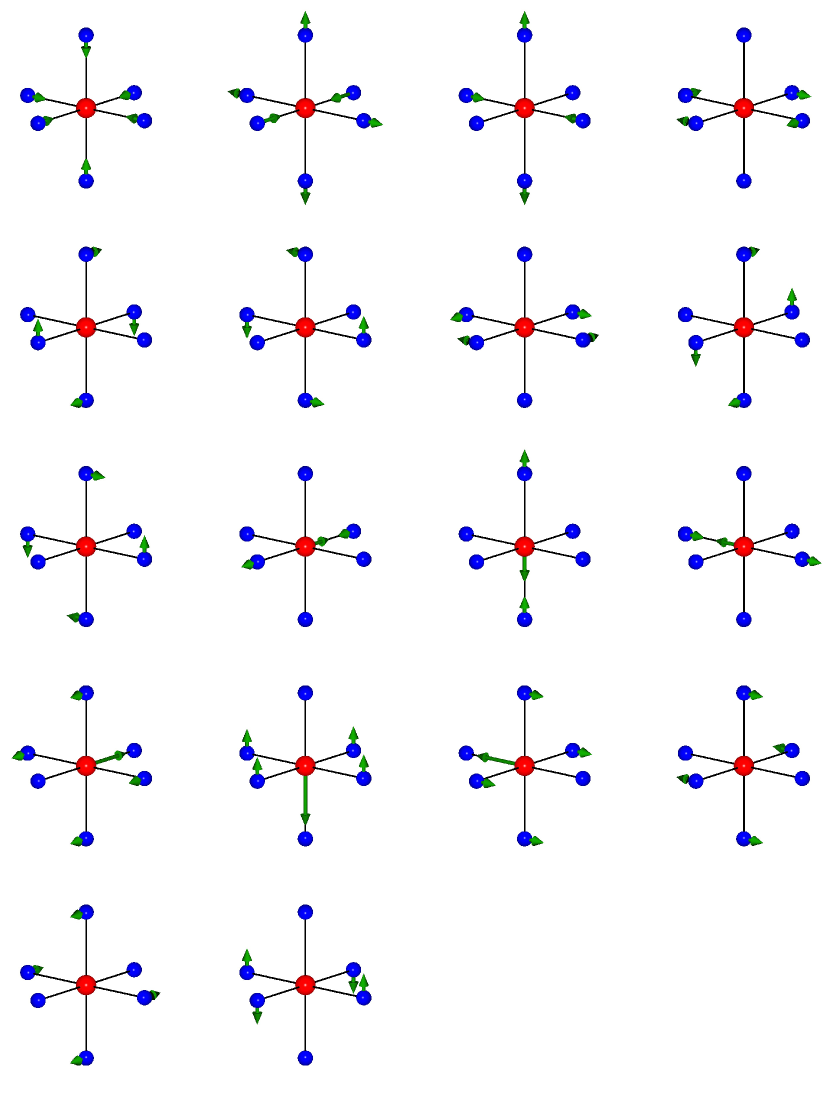
Figure 3: Octahedral modes transforming as the irreducible representations of the point group. The three $T_{1u}$ modes which shift the octahedron have been removed. Reading from left to right and top to bottom, the modes are $A_{1g},E_{g},T_{1g},T_{2g},2T_{1u},\textrm{and }T_{2u}$.

The octahedral slave representation can be decomposed into $\Gamma=A_{1g}\oplus E_{g}\oplus T_{1g}\oplus T_{2g}\oplus 2T_{1u}\oplus T_{2u}$, where we have remove a $T_{1u}$ manifold which rigidly shifts the octahedron. One can then form product representations in a given octahedron, showing that there are 29 unique products at third order and 153 unique products at fourth order. This will be the case for both Pb and Te centered octahedron. Nontranslational symmetry elements will not generate any translationally inequivalent slave clusters. Employing the translation group, one can demonstrate that some of the terms are redundant. In particular, two terms will be removed at third order, and four terms will be removed at fourth order. The final result is that there are 56 terms at third order and 302 terms at fourth order, for a total of 358 terms up to fourth order and within next-nearest neighbor range.

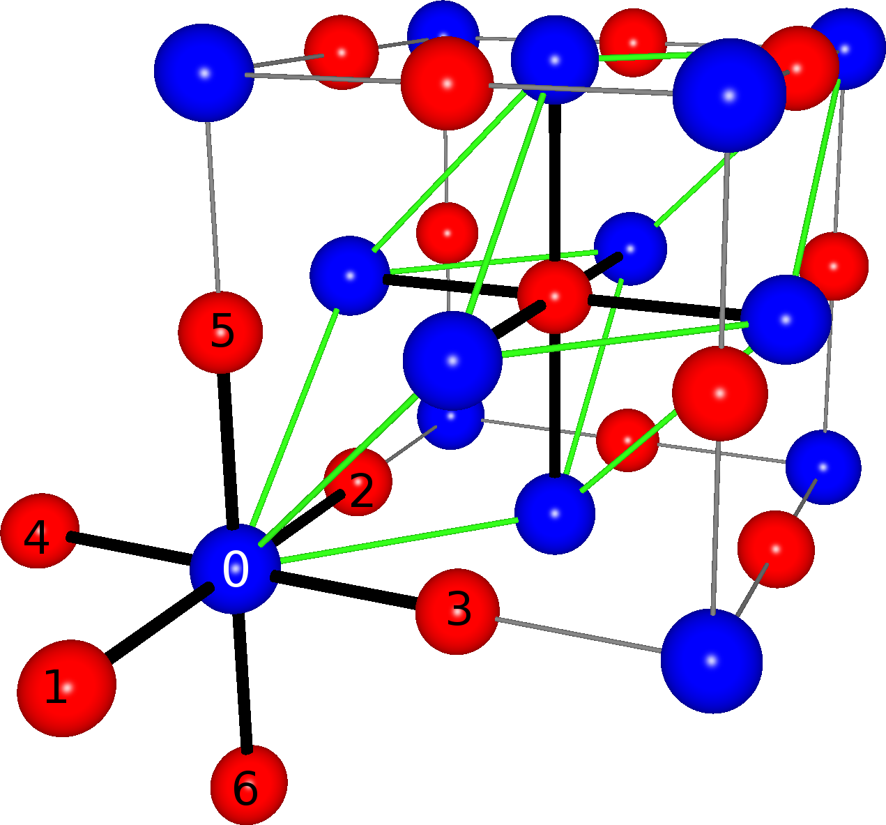
Figure 4: A section of the rock salt structure. The primitive unit cell is given in green. The two slave clusters associated with the primitive unit cell are denoted by atoms connected with bold lines. The octahedral numbering convention is shown.

The third order products and corresponding coefficients are listed in table III, while fourth order terms are listed in table 2. It should be noted that within a given product some of the identity representations are redundant or zero due to the fact that we are dealing with self-products. For example, $E_{g}\otimes E_{g}\otimes E_{g}\otimes E_{g}=5E_{g}\oplus 3A_{2g}\oplus 3A_{1g}$, but only one of the three $A_{1g}$ representations is unique when projecting the displacement product vector. It is important to note the phase convention we chose in constructing the Clebsch-Gordan coefficients. The vectors in each product subspace are labeled from $1\dots N$ when taking the following ordering:

$$|1,0,0,0,0,\cdots\rangle,|0,1,0,0,0,\cdots\rangle,\cdots$$ (38)

In tables III and 2 we list the vector which was used to project onto the identity, and this sets the phase convention for our Clebsch-Gordan coefficients wich can straightforwardly be constructed.

Product	Phase	Pb-centered $\Phi$	Te-centered $\Phi$
$T_{2g}\otimes 2T_{1u}\otimes T_{2u}$	32, 45	-0.059,-0.048	-0.033,-0.043
$E_{g}\otimes T_{1g}\otimes T_{1g}$	1	-0.011	0.001
$T_{1g}\otimes T_{1g}\otimes T_{2g}$	16	0.002	-0.002
$A_{1g}\otimes E_{g}\otimes E_{g}$	1	0.074	-0.002
$T_{2g}\otimes 2T_{1u}\otimes 2T_{1u}$	38, 59, 84	-0.276,-0.245,-0.524	-0.129,-0.148,-0.284
$T_{1g}\otimes 2T_{1u}\otimes T_{2u}$	45, 54	0.102,-0.084	0.022,-0.025
$A_{1g}\otimes T_{2u}\otimes T_{2u}$	5	-0.01	N/A
$T_{2g}\otimes T_{2g}\otimes T_{2g}$	6	-0.003	0.002
$E_{g}\otimes 2T_{1u}\otimes T_{2u}$	20, 29	-0.041,0.067	0.008,0.001
$A_{1g}\otimes 2T_{1u}\otimes 2T_{1u}$	4, 15, 22	-1.849,1.288,0.635	-0.282,0.188,0.091
$E_{g}\otimes T_{2g}\otimes T_{2g}$	14	-0.003	-0.006
$T_{1g}\otimes 2T_{1u}\otimes 2T_{1u}$	6	-0.022	0.006
$E_{g}\otimes E_{g}\otimes E_{g}$	4	-0.035	0.005
$E_{g}\otimes 2T_{1u}\otimes 2T_{1u}$	4, 22, 51	-2.341,0.941,1.754	0.573,-0.197,-0.449
$T_{2g}\otimes T_{2u}\otimes T_{2u}$	2	0.002	-0.007
$E_{g}\otimes T_{1g}\otimes T_{2g}$	5	0.018	-0.005
$A_{1g}\otimes T_{2g}\otimes T_{2g}$	9	-0.002	0.006
$A_{1g}\otimes A_{1g}\otimes A_{1g}$	1	0.01	N/A
$A_{1g}\otimes T_{1g}\otimes T_{1g}$	1	-0.011	-0.004
$E_{g}\otimes T_{2u}\otimes T_{2u}$	10	0.008

Table 1: Nonzero third order products and the corresponding expansion coefficients. The second column lists which product vector was used to project the identity and create the Clebsch-Gordan coefficients for each corresponding coefficient $\Phi$. Terms designated N/A were those removed by the translation group.

IV Computing expansion coefficients for PbTe

Having determined the slave mode expansion up to 4^th order and within next-nearest neighbor, the slave mode coefficients must be computed. In general, there are be many approaches to execute this task. Firstmost, as described above, we will assume that the harmomic terms have been computed using tranditional approaches for computing phonons from first-principles, such as density functional perturbation theoryBaroni et al. (2001) or finite displacement supercell approachesAlfe (2009); Kunc and Martin (1982). Therefore, we are only concerned with computing the third and fourth order terms. An obvious approach would be to construct a large data set of atomic displacements in the anharmonic regime and compute the corresponding energies using DFT. This dataset may then be used to fit the slave mode expansion coefficients using standard procedures. The drawback of such an approach is that one is always faced with the problems of overfitting or incuding data which which is beyond fourth order. While there are standard statistical methods to address such problems, we believe other approaches are likely more straightforward. Another approach would be to compute individual expansion coefficients in the direct expansion (ie. equation 2), analagous to what is done for the harmonic case in phonons. One could either use the $2N+1$ theorem from density functional perturbation theoryGonze and Vigneron (1989); Debernardi et al. (1995); Deinzer et al. (2003), or a supercell approach using finite displacements could be used. We will opt for the latter in this work.

The computed direct expansion terms are only of limited use given that small errors within the numerical implementation of DFT will prevent the computed direct terms from satisfying all the necessary symmetries. However, there is a linear relation between the slave mode coefficients and the direct expansion coefficients (see equation 37 for an example). Therefore, one simply needs to compute enough direct coefficients such that the slave mode coefficients are uniquely defined. In the case of PbTe, we will need to compute at least 56 direct coefficients at third order and 302 at fourth order. In practice, it is desirable to compute more than the minimum number to minimize the effects of error within the DFT finite difference calculations.

These linear relations will properly average out any small noise from the direct coefficients and enforce all symmetry relations. What should be apparent is that these relations assume a truncation in the range of the slave modes. This is clearly an approximation which relies on a sufficient degree of locality in order to be accurate, and we will show that our truncation of an octahdron for PbTe is reasonable. The other major potential source of error is the convergence of the direct finite difference terms which will be dealt with below. While it would be desirable to directly compute the slave mode coefficients, this is not straightforward as the slave modes are not orthogonal.

IV.1 DFT runs and Finite Difference

As outlined above, the direct expansion coefficient will be computed with finite difference. Given that the forces are known from the Hellman-Feynman TheoremMartin (2008), the first derivatives will all be known for a given DFT computation. Using a central finite difference, a derivative containing up to four variables can generically be written:

$$\frac{\partial^{n}E}{\partial q_{\alpha}^{h}\partial q_{\beta}^{i}\partial q_{\gamma}^{j}\partial q_{\delta}^{k}}=\frac{\partial^{n-1}F_{\alpha}}{\partial q_{\alpha}^{h-1}\partial q_{\beta}^{i}\partial q_{\gamma}^{j}\partial q_{\delta}^{k}}$$

$$\approx\frac{1}{2\Delta}\frac{\partial^{n-2}}{\partial q_{\alpha}^{h-1}\partial q_{\beta}^{i-1}\partial q_{\gamma}^{j}\partial q_{\delta}^{k}}\left[F_{\alpha}(q_{\beta}+\Delta)-F_{\alpha}(q_{\beta}-\Delta)\right]$$

$$\approx\frac{1}{4\Delta^{2}}\frac{\partial^{n-3}}{\partial q_{\alpha}^{h-1}\partial q_{\beta}^{i-1}\partial q_{\gamma}^{j-1}\partial q_{\delta}^{k}}\left[F_{\alpha}(q_{\beta}+\Delta,q_{\gamma}+\Delta)-\right.$$

$$\hskip 14.22636ptF_{\alpha}(q_{\beta}-\Delta,q_{\gamma}+\Delta)-F_{\alpha}(q_{\beta}+\Delta,q_{\gamma}-\Delta)$$

$$\hskip 14.22636pt\left.+F_{\alpha}(q_{\beta}-\Delta,q_{\gamma}-\Delta)\right]$$

$$\approx\dots$$

$$=\frac{1}{{(2\Delta)}^{n-1}}\sum_{n_{\alpha}=0}^{h-1}\sum_{n_{\beta}=0}^{i}\sum_{n_{\gamma}=0}^{j}\sum_{n_{\delta}=0}^{k}{h-1\choose n_{\alpha}}{i\choose n_{\beta}}{j\choose n_{\gamma}}{k\choose n_{\delta}}$$

$$(-1)^{n_{\alpha}+n_{\beta}+n_{\gamma}+n_{\delta}}F_{\alpha}(q_{\alpha}+(h-1-2n_{\alpha})\Delta,q_{\beta}+(i-2n_{\beta})\Delta,$$

$$q_{\gamma}+(j-2n_{\gamma})\Delta,q_{\delta}+(k-2n_{\delta})\Delta)$$ (39)

with $\alpha,\beta,\gamma,\delta$ label both the atom and the displacement vector, $n=h+i+j+k$ which label the order of the derivative, $F$ is force, and $\Delta$ is the finite difference displacement. For a third order term, four DFT computations will be needed, while eight will be needed for a fourth order term.

The forces are computed within the framework of Density Functional Theroy which is carried out using the generalized gradient approximation (GGA) by Perdew and WangPerdew et al. (1996) as implemented in the Vienna ab initio simulation package (VASP) Kresse and Hafner (1993, 1994); Kresse and Furthmuller (1996a, b); Kresse and Joubert (1999). Gamma centered k-meshes depending on the supercell size are applied and a $3\times 3\times 3$ mesh is used for the smallest 64-atom supercell. Charge self-consistency is performed until the energy is converged to within $10^{-5}$ eV, and a plane wave cutoff of $175-350eV$ was used depending on the particular computation. Spin-orbit coupling was not utilized.

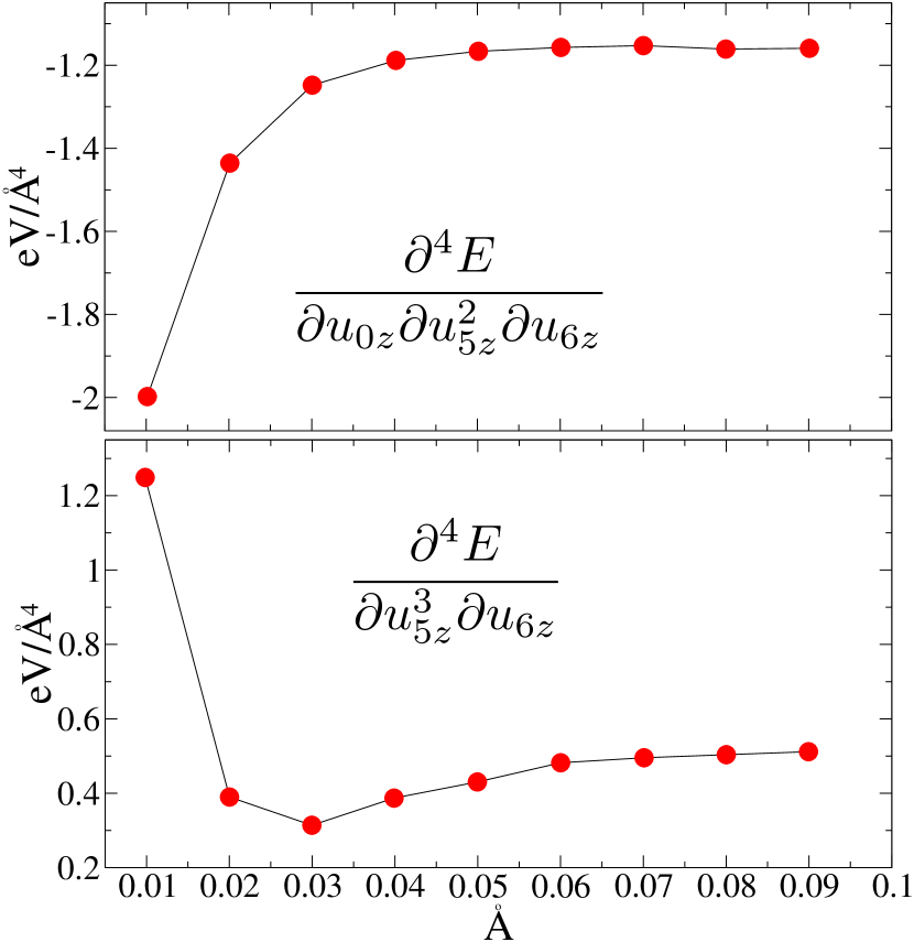
Figure 5: Fourth order derivatives computed using central step finite difference as a function of $\Delta$ for a conventional supercell choice of $2\times 2\times 3$ (ie. 96 atoms).

In order to be sure the direct coefficients are robustly computed within finite difference, one must test for convergence with respect to the displacement size $\Delta$ in addition to the supercell size. If $\Delta$ is chosen to be too small, a probibitive planewave cuttoff and k-point mesh will be required, while if it is too large higher order terms will taint the computation. Therefore, there will be an optimum $\Delta$ which will be both efficient and accurate, and this will strongly depend on the order of the derivative. In order to illustrate this point, the values of two different fourth order expansion coefficients are plotted as a function of $\Delta$ (see figure 5). A clear platuea emerges in both cases, revealing a robust value for $\Delta$. After examining a wide range of different types of direct coefficients, we found that $\Delta=0.01\AA$ is reliable for third order while $\Delta=0.07\AA$ is reliable for fourth order. Supercell size must also be studied to be sure that images are not interacting with one another. The minimum supercell dimension that was used was twice the conventional (ie. cubic) cell size, while the maximum was six times the conventional cell size. In order to illustrate this, we plot two fourth order coeefficients as a function of unit cell size along a particular dimension (see figure 6), demonstrating that the changes in the coefficients are diminishing with increasing cell size. Our convergence criteria for supercell dimension was determined based on the largest finite difference coefficient at a specific order, and for third order the unit cell size was increased until changes were within 0.01 $eV/\AA^{3}$ while the threshold was 0.1$eV/\AA^{4}$ for fourth order.

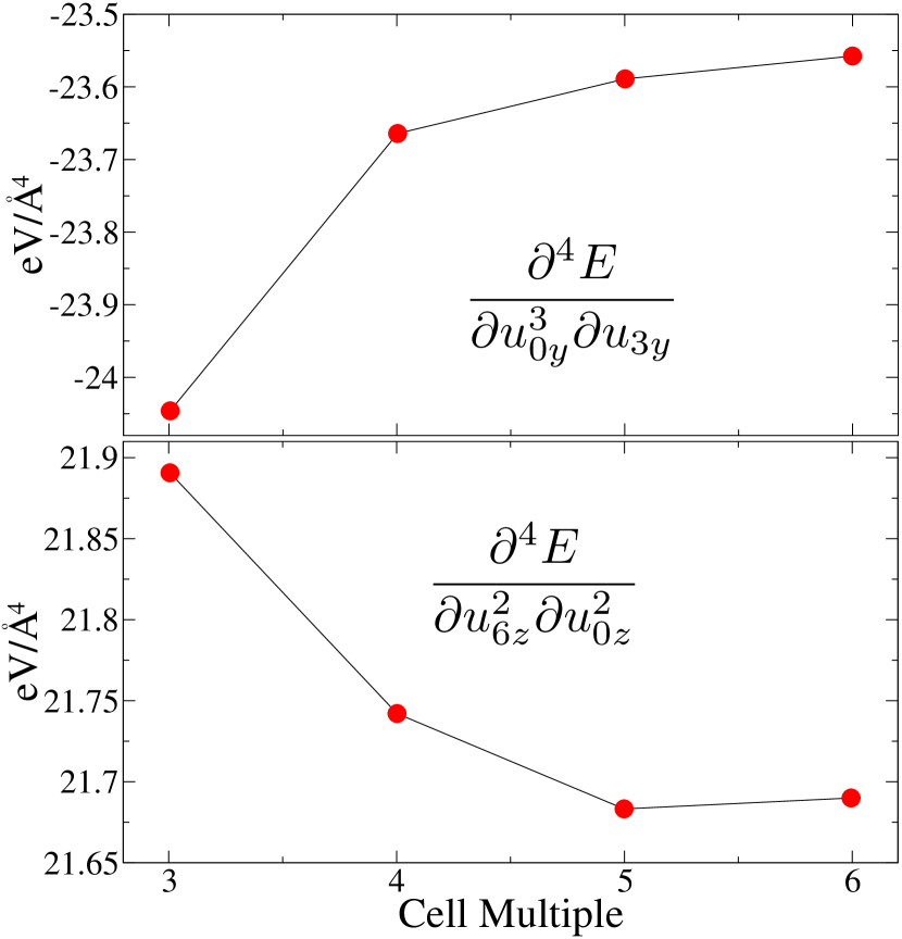
Figure 6: Fourth order derivatives computed using central step finite difference as a function of conventional supercell size in the $y$-direction for $\Delta=0.07\AA$

Product	Phase	Pb-centered $\Phi$	Te-centered $\Phi$
$E_{g}\otimes E_{g}\otimes T_{2g}\otimes T_{2g}$	14, 32	-0.043, -0.034	0.008, 0.01
$T_{2g}\otimes T_{2g}\otimes 2T_{1u}\otimes T_{2u}$	83, 151, 36, 27	0.938, -0.681, 0.031, -0.05	-1.014, 0.742, 0.088, -0.077
$T_{2u}\otimes T_{2u}\otimes T_{2u}\otimes T_{2u}$	1, 5	0.017, 0.003	-0.015, 0.001
$E_{g}\otimes T_{1g}\otimes T_{1g}\otimes T_{2g}$	35	-0.0	0.003
$T_{1g}\otimes T_{1g}\otimes T_{1g}\otimes T_{2g}$	25	-0.007	-0.001
$A_{1g}\otimes T_{2g}\otimes T_{2g}\otimes T_{2g}$	6	0.001	0.002
$A_{1g}\otimes E_{g}\otimes T_{1g}\otimes T_{1g}$	14	0.029	-0.01
$T_{1g}\otimes T_{2g}\otimes T_{2g}\otimes T_{2g}$	9	-0.002	0.007
$E_{g}\otimes E_{g}\otimes T_{1g}\otimes T_{2g}$	14	-0.121	0.047
$2T_{1u}\otimes 2T_{1u}\otimes 2T_{1u}\otimes 2T_{1u}$	533, 1, 1044, 11, 22, 59, 606, 130, 15, 1037, 522	-8.18, 7.405, -3.203, 10.942, 45.45, -10.874, 13.284, -35.053, -2.019, 10.804, -28.53	17.113, 1.528, 7.597, -31.941, -10.505, 30.786, -31.418, 15.514, 7.908, -6.578, N/A
$T_{1g}\otimes T_{1g}\otimes T_{2g}\otimes T_{2g}$	73, 41, 11	0.003, 0.102, -0.005	0.0, -0.102, 0.003
$A_{1g}\otimes A_{1g}\otimes A_{1g}\otimes A_{1g}$	1	0.002	-0.001
$E_{g}\otimes T_{1g}\otimes T_{2g}\otimes T_{2g}$	47	0.002	0.005
$T_{2g}\otimes T_{2g}\otimes T_{2g}\otimes T_{2g}$	41, 5	0.017, 0.001	-0.017, -0.002
$T_{1g}\otimes T_{1g}\otimes T_{1g}\otimes T_{1g}$	41, 45	0.018, 0.003	-0.014, 0.001
$E_{g}\otimes T_{1g}\otimes 2T_{1u}\otimes T_{2u}$	54, 108, 1, 8	0.172, -0.297, 0.467, -0.001	-0.11, 0.195, -0.304, -0.006
$E_{g}\otimes T_{2g}\otimes 2T_{1u}\otimes 2T_{1u}$	89, 16, 146, 102	-1.391, 1.118, -0.416, 0.398	1.716, -0.56, 0.801, -0.685
$2T_{1u}\otimes T_{2u}\otimes T_{2u}\otimes T_{2u}$	18, 83	0.038, 0.054	-0.018, -0.018
$T_{1g}\otimes T_{1g}\otimes 2T_{1u}\otimes 2T_{1u}$	317, 53, 29, 95, 292, 152, 183, 155, 289	2.214, 0.136, 0.021, 0.089, -0.004, 0.833, 0.051, -2.914, -0.013	-1.801, -0.238, -0.05, -0.137, 0.092, -0.584, -0.107, 2.242, -0.046
$A_{1g}\otimes T_{2g}\otimes T_{2u}\otimes T_{2u}$	21	0.007	0.005
$E_{g}\otimes E_{g}\otimes E_{g}\otimes E_{g}$	4	0.024	-0.01
$E_{g}\otimes T_{1g}\otimes 2T_{1u}\otimes 2T_{1u}$	16, 192, 111, 167	1.062, 3.955, -2.932, -2.859	-0.674, -2.289, 1.606, 1.627
$A_{1g}\otimes T_{1g}\otimes T_{1g}\otimes T_{2g}$	8	-0.001	0.002
$T_{1g}\otimes T_{1g}\otimes T_{2u}\otimes T_{2u}$	77, 5, 12	0.006, 0.102, -0.005	0.001, -0.098, -0.002
$E_{g}\otimes T_{2g}\otimes 2T_{1u}\otimes T_{2u}$	17, 99, 71, 21	0.226, 0.207, -0.204, 0.248	-0.069, 0.098, 0.198, -0.363
$E_{g}\otimes E_{g}\otimes T_{1g}\otimes T_{1g}$	9, 28	0.071, -0.106	-0.026, 0.039
$A_{1g}\otimes T_{1g}\otimes 2T_{1u}\otimes T_{2u}$	10, 40	-0.263, -0.359	0.071, 0.118
$A_{1g}\otimes T_{2g}\otimes 2T_{1u}\otimes 2T_{1u}$	102, 38, 41	-0.905, 0.882, -1.902	0.675, -0.724, 1.459
$T_{1g}\otimes T_{1g}\otimes 2T_{1u}\otimes T_{2u}$	83, 39, 107, 74	0.986, -0.009, 0.025, -0.718	-0.918, 0.02, -0.027, 0.662
$E_{g}\otimes T_{2g}\otimes T_{2u}\otimes T_{2u}$	29	-0.003	0.002
$2T_{1u}\otimes 2T_{1u}\otimes 2T_{1u}\otimes T_{2u}$	30, 540, 280, 306, 142, 7	2.355, -1.842, -0.811, 4.857, -3.446, -1.88	-8.661, 4.674, 3.853, -10.649, 6.226, 4.979
$A_{1g}\otimes A_{1g}\otimes 2T_{1u}\otimes 2T_{1u}$	8, 11, 29	0.598, -0.725, 0.145	0.078, -0.158, 0.096
$A_{1g}\otimes E_{g}\otimes E_{g}\otimes E_{g}$	1	0.03	0.0
$A_{1g}\otimes E_{g}\otimes T_{2u}\otimes T_{2u}$	5	0.028	-0.005
$A_{1g}\otimes E_{g}\otimes T_{1g}\otimes T_{2g}$	10	0.17	-0.06
$A_{1g}\otimes E_{g}\otimes 2T_{1u}\otimes 2T_{1u}$	29, 54, 51	-2.974, -3.915, 2.377	0.315, 0.165, 0.021
$A_{1g}\otimes A_{1g}\otimes T_{1g}\otimes T_{1g}$	5	-0.018	0.001
$A_{1g}\otimes T_{1g}\otimes 2T_{1u}\otimes 2T_{1u}$	89	0.831	-0.347
$E_{g}\otimes E_{g}\otimes 2T_{1u}\otimes 2T_{1u}$	130, 47, 72, 11, 15 116	-0.093, -2.737, -0.91, -0.678, -0.85, 1.64	0.255, 0.112, -0.052, -0.397, 0.175, N/A
$A_{1g}\otimes A_{1g}\otimes T_{2g}\otimes T_{2g}$	1	-0.013	N/A
$A_{1g}\otimes T_{2g}\otimes 2T_{1u}\otimes T_{2u}$	10, 23	-0.146, -0.237	0.108, 0.16
$E_{g}\otimes E_{g}\otimes T_{2u}\otimes T_{2u}$	18, 36	0.043, -0.037	-0.009, 0.007
$A_{1g}\otimes E_{g}\otimes 2T_{1u}\otimes T_{2u}$	34, 20	0.754, -0.283	-0.344, 0.133
$T_{1g}\otimes T_{2g}\otimes 2T_{1u}\otimes T_{2u}$	83, 74, 22, 143, 155, 72, 79, 113	1.913, -1.372, -0.02, 0.04, -0.07, -0.004, -0.056, -0.026	-2.0, 1.461, -0.015, -0.052, 0.039, -0.027, 0.029, 0.038
$E_{g}\otimes T_{1g}\otimes T_{2u}\otimes T_{2u}$	2	-0.001	-0.001
$T_{2g}\otimes T_{2g}\otimes T_{2u}\otimes T_{2u}$	24, 77, 41	-0.001, 0.003, 0.098	-0.007, -0.002, -0.105
$2T_{1u}\otimes 2T_{1u}\otimes T_{2u}\otimes T_{2u}$	198, 99, 28, 264, 135, 72, 87, 20, 261	-0.194, -3.438, 0.63, 0.415, -0.47, 1.251, 0.813, 0.409, 2.36	0.326, 3.335, -0.834, 0.041, 0.531, -1.225, 0.133, 0.09, -2.28
$T_{2g}\otimes T_{2g}\otimes 2T_{1u}\otimes 2T_{1u}$	306, 196, 1, 317, 66, 8, 310, 162, 45	-2.88, -0.216, 0.857, 2.154, -0.093, -0.048, -0.015, 0.067, -0.118	2.73, -0.047, -0.8, -2.083, -0.056, -0.106, -0.125, 0.226, N/A
$T_{1g}\otimes T_{2g}\otimes 2T_{1u}\otimes 2T_{1u}$	15, 95, 120, 221, 18, 324, 117	3.295, -0.036, -0.071, -0.081, -7.9, -5.024, 0.104	-3.6, -0.228, -0.166, -0.148, 8.646, 5.441, 0.098
$A_{1g}\otimes A_{1g}\otimes T_{2u}\otimes T_{2u}$	1	-0.014	-0.0
$A_{1g}\otimes E_{g}\otimes T_{2g}\otimes T_{2g}$	9	0.018	-0.013
$T_{1g}\otimes T_{2g}\otimes T_{2u}\otimes T_{2u}$	60, 73	0.002, -0.202	-0.005, 0.205
$A_{1g}\otimes A_{1g}\otimes E_{g}\otimes E_{g}$	4	0.027	0.003
$E_{g}\otimes E_{g}\otimes 2T_{1u}\otimes T_{2u}$	6, 29	-0.288, -0.326	-0.008, 0.021

Table 2: Nonzero fourth order products and the corresponding expansion coefficients. The second column lists which product vector was used to project the identity and create the Clebsch-Gordan coefficients for each corresponding coefficient $\Phi$.

IV.2 Slave mode expansion coeefficients

We have computed 70 direct expansion coefficients at 3^rd order and 427 at 4^th order. This exceeds the 56 slave mode coefficients at 3^rd order and 302 coeefficients at 4^th order, and therefore we have an overdetermined set of equations. Singular value decomposition can then be used to find the optimum solution in terms of least squares, and this will yield a unique solution for the slave mode coefficients. The third and fourth order terms are plotted in figure 7. At third order, the Pb-centered slave modes have substantially larger coefficients than the Te-centered slave modes, while the differences are less pronounced for fourth order. The values of each slave mode coefficient are also listed in tables III and 2.

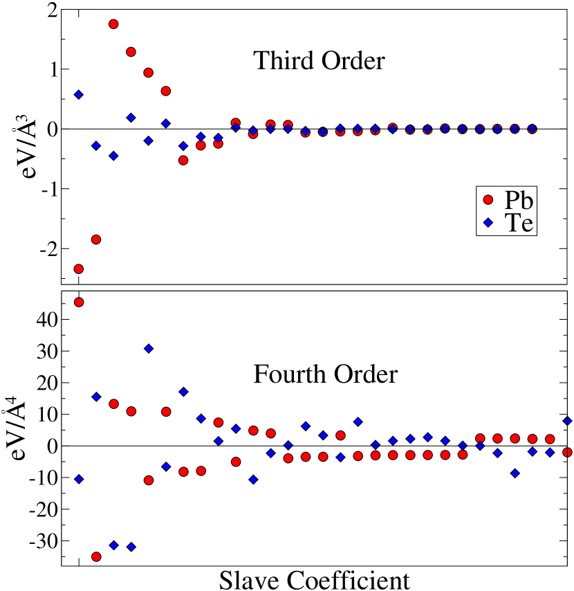
Figure 7: A plot of the third and fourth order slave mode product coeefficients $\Phi$. The values are ordered in decreasing magnitude for the Pb-centered coefficients, and the same absolute ordering is used for the Te-centered coefficients.

V Assessing the expansion

Having computed the slave mode expansion coefficients up to fourth order and within next nearest neighbor interaction, we now evaluate the overall reliability of our expansion. The major point of concern in the method we have employed to compute the slave mode coefficients is whether or not the slave mode expansion is sufficiently converged within the octahedron or if non-negligible terms beyond the octahedron are present. A potent test to address this issue is to use the slave mode expansion to compute energy, stress, and phonons as a function of lattice strain. It should be emphasized that our slave mode expansion is performed in the absence of any strain, but if our cluster is sufficiently large the expansion will be able to to be used to compute the energetics under strain. Given that strain will amplify the coupling to long range interactions, and that it is straightforward to compute the answer to these tests using DFT, this serves as an ideal testbed of our method. PbTe is sufficiently polar such that there be long range fields which will cause a non-negligible splitting of the optical modes near the $\Gamma$-point. These can be straightforwardly taken into account via Born effective chargesBaroni et al. (2001), but we do not include them in this study.

The first test is to compute the energy and the stress as a function of strain (see figure 8). As shown, there is remarkable agreement in the stress for strains as high as 7% and even higher for the energy. At 10% strain there is an error of roughly 8% in the stress. This favorable agreement suggests that longer range terms are not substantial.

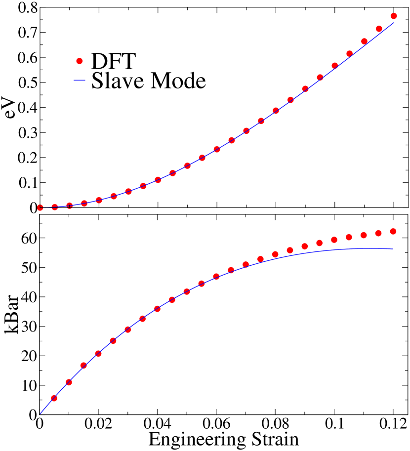
Figure 8: Top Panel: Energy as a function of triaxial engineering strain. Bottom Panel: True Stress as a function of triaxial engineering strain.

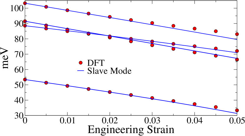
Figure 9: L-point phonon frequencies as a function of triaxial engineering strain.

A more stringent test is to compute the phonons as a function of strain. We begin by computing the L-point phonons as a function of strain (see figure 9). As shown, there is remarable agreement up to 5% strain.

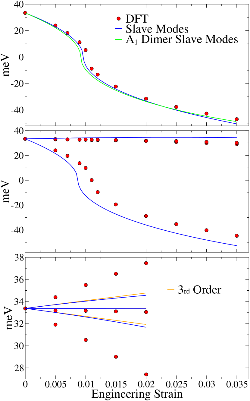
Figure 10: $\Gamma$-point optical phonon frequencies as a function of different engineering strain states: triaxial (top panel), uniaxial (middle panel), and shear $\gamma_{xy}$ (bottom panel).

Another test of phonons under strain is the $\Gamma$-point optical modes. This mode is of particular interest in the context of PbTe as it displays anomolous temperature dependenceJensen et al. (2012); Delaire et al. (2011); Chen et al. (2013). We compute energy of the $\Gamma$-point optical modes as a function of triaxial, uniaxial, and shear strain (see figure 10). In the case of triaxial strain, the slave mode expansion precisely captures the formation of a soft-mode. In the case of uniaxial strain, the slave mode expansion is highly accurate for small strains and properly captures the symmetry breaking of the optical modes. However, errors are apparent for the prediction of the soft mode at larger strains, though the error is relatively constant beyond 1.5%. In the case of shear strain, the splitting of the optical modes is underpredicted using the slave modes, though the error is still within reason in this range of strain. Nonetheless, the troubling aspect of this result is that it does not have the correct slope in the limit of small strains. Given that there is little difference in going from third to fourth order coefficients, this is likely a symptom of a longer range terms that are not present in our expansion. Fortunately, the overall magnitude of this effect is rather small, and these errors will likely be unimportant in most scenarios. The final test will be the displacement of a single Pb atom in a 216-atom supercell (see figure 11). The slave mode expansion is highly accurate even at displacements beyond 1.2 $\AA$. We believe these benchmarks demonstrate that our expansion is robust.

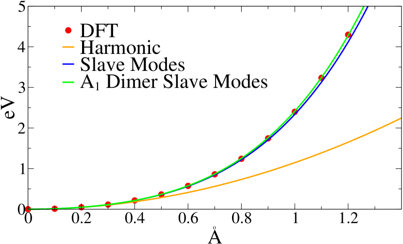
Figure 11: Energy as a function of displacing a single Pb atom in a 216 atom supercell along the $<-3,1,1>$ direction.

VI Minimal Model

Above we have demonstrated that our slave mode expansion accurately reproduces many key quantities. Nonetheless, it would be strongly desirable if we could somehow extract a minimal model of anharmoncity. It would be intuitive for the nearest-neighbor terms to be larger than the next nearest neighbor terms. When choosing the octahedral cluster, the nearest and next-nearest neighbor terms will be mixed. However, they can be seperated. We will start by considering the dimer slave cluster of Pb-Te, where we will use the $C_{4v}$ symmetry along the bond. Given that this case is three dimensional, the representation for the dimer will have six degrees of freedom, and projecting them onto the irreducible representations of the point group yields the following representation: $\Gamma=2E\oplus 2A_{1}$ The representation for the modes which shift the dimer in the $x,y,z$ directions can be chosen as one set of $E\oplus A_{1}$ and this must be removed leaving the following slave mode representation: $E\oplus A_{1}$. These modes can be explicitly constructed as follows:

$$\phi_{A_{1}} =\frac{1}{\sqrt{2}}(u_{Te,x}-u_{Pb,x})$$

$$\phi_{E^{(1)}} =\frac{1}{\sqrt{2}}(u_{Te,y}-u_{Pb,y})\hskip 5.69054pt\phi_{E^{(2)}}=\frac{1}{\sqrt{2}}(u_{Te,z}-u_{Pb,z})$$ (40)

In this case we chose a cluster centered on a bond where the $x$-axis aligns with the $4$-fold rotation axis. At third order there will be two terms: $\phi_{A_{1}}^{3}$ and $\phi_{A_{1}}\left(\phi_{E^{(1)}}^{2}+\phi_{E^{(2)}}^{2}\right)$. At fourth order there will be four terms:$\phi_{A_{1}}^{4}$ and $\phi_{A_{1}}^{2}\left(\phi_{E^{(1)}}^{2}+\phi_{E^{(2)}}^{2}\right)$ and $\phi_{E^{(1)}}^{2}\phi_{E^{(2)}}^{2}$ and $\phi_{E^{(1)}}^{4}+\phi_{E^{(2)}}^{4}$. The $O_{h}$ symmetry center will then generate five more equivalent set of slave mode products for each case, one for each bond. We can add these terms to our original set of products in tables III and 2, but then we will need to remove two products at third order and four products at fourth order to regain an irreducible space. This is equivalent to performing a unitary transformation within the product space. After reconstructing the expansion coefficients for this new set of products, we then orthogonalize all of the products to the dimer mode products. This physically motivated choice of phase convention in the product space achieves the goal of creating a minimal model in that there is now one dominant term at both third and fourth order (see figure 12). The dominant terms correspond to $\phi_{A_{1}}^{3}$ at third order and $\phi_{A_{1}}^{4}$ at fourth order. These two terms can be used to explicitly write a minimal model for the potential (we drop for $A_{1}$ index below):

$$V=V_{H}+$$

$$\Phi_{3}\sum_{\mathbf{R}}(-\phi_{\mathbf{R}x_{-}}^{3}+\phi_{\mathbf{R}x_{+}}^{3}-\phi_{\mathbf{R}y_{-}}^{3}+\phi_{\mathbf{R}y_{+}}^{3}-\phi_{\mathbf{R}z_{-}}^{3}+\phi_{\mathbf{R}z_{+}}^{3})+$$

$$\Phi_{4}\sum_{\mathbf{R}}(\phi_{\mathbf{R}x_{-}}^{4}+\phi_{\mathbf{R}x_{+}}^{4}+\phi_{\mathbf{R}y_{-}}^{4}+\phi_{\mathbf{R}y_{+}}^{4}+\phi_{\mathbf{R}z_{-}}^{4}+\phi_{\mathbf{R}z_{+}}^{4})$$ (41)

and:

$$\begin{array}[]{lr}\phi_{\mathbf{R}z_{-}}=\frac{1}{\sqrt{2}}(u^{\mathbf{R}+\bf{a_{1}}}_{Te,z}-u^{\mathbf{R}}_{Pb,z})&\phi_{\mathbf{R}z_{+}}=\frac{1}{\sqrt{2}}(u^{\mathbf{R}+\bf{a_{2}+a_{3}}}_{Te,z}-u^{\mathbf{R}}_{Pb,z})\\ \phi_{\mathbf{R}x_{-}}=\frac{1}{\sqrt{2}}(u^{\mathbf{R}+\bf{a_{2}}}_{Te,x}-u^{\mathbf{R}}_{Pb,x})&\phi_{\mathbf{R}x_{+}}=\frac{1}{\sqrt{2}}(u^{\mathbf{R}+\bf{a_{1}+a_{3}}}_{Te,x}-u^{\mathbf{R}}_{Pb,x})\\ \phi_{\mathbf{R}y_{-}}=\frac{1}{\sqrt{2}}(u^{\mathbf{R}+\bf{a_{3}}}_{Te,y}-u^{\mathbf{R}}_{Pb,y})&\phi_{\mathbf{R}y_{+}}=\frac{1}{\sqrt{2}}(u^{\mathbf{R}+\bf{a_{1}+a_{2}}}_{Te,y}-u^{\mathbf{R}}_{Pb,y})\end{array}$$ (45)

Where $V_{H}$ is the harmonic part of the potential, $\phi$ are the slave modes for the dimer, $u$ are the atomic displacements, and $\bf{a_{i}}$ are the primitive lattice vectors of PbTe: ${\bf a_{1}}=a/2(1,1,0)$, ${\bf a_{2}}=a/2(0,1,1)$, and ${\bf a_{3}}=a/2(1,0,1)$. There are six dimer slave modes per primitive unit cell, one corresponding to each Pb-Te octahedral bond, and these are simply a displacement difference between corresponding vectors of Pb and Te. The values for the expansion coefficients are found to be $\Phi_{3}=2.68eV/{\AA}^{3}$ and $\Phi_{4}=3.70eV/{\AA}^{4}$, respectively. We can test these two parameters by recomputing the optical modes under strain (see figure 10) and the energy of displacing a single atom (see figure 11), displaying excellent agreement. This minimal model has already been used to capture the anomolous temperature dependence of the phonon spectra in PbTeChen et al. (2013).

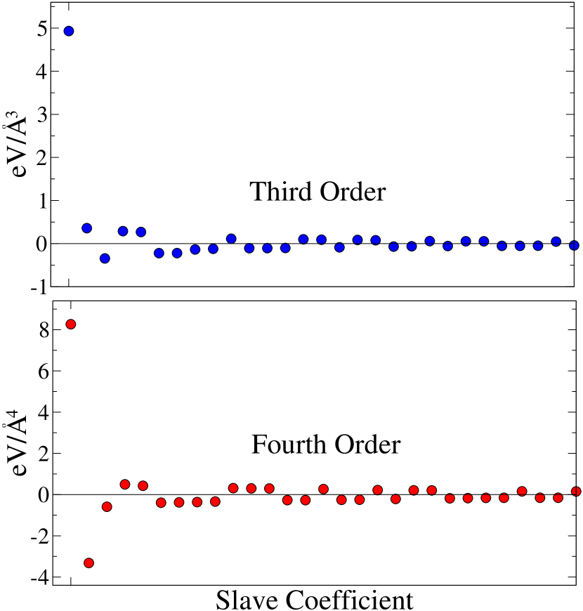
Figure 12: A plot of the transformed third and fourth order slave mode product coeefficients $\Phi^{\prime}$. The values are ordered in decreasing magnitude.

There is one other term at fourth order which, though smaller, stands out among the other terms. This corresponds to $\phi_{A_{1}}^{2}\left(\phi_{E^{(1)}}^{2}+\phi_{E^{(2)}}^{2}\right)$ and has a coefficient of $-1.37eV/{\AA}^{4}$.

VII Conclusions

In conclusion, we have introduced a new approach to perform a Taylor series expansion of the total energy as a function of the nuclear displacements. The novelty of our approach is the formation of new variables (ie. slave modes) which transform like the irreducible representations of the space group while satisfying the homogeneity of free space, and these benefits are gained at the expense of increasing the dimensionality of the space. We used a finite difference approach to compute the slave mode coefficients, and accurately determined all 358 terms within fourth order and next nearest neighbor coupling. Examining the energy, stress, and phonons under lattice strain indicated that our expansion parameters are robust and that terms outside of the octahedron are relatively small. Furthermore, we have introduced an additional approach to perform a unitary transformation which allows us to accurately compress 56 cubic terms to one term and the 302 quartic terms to one term. This two parameter model of anharmonicity in PbTe has already been separately used to compute the temperature dependent phonon spectrum in the classical limit, resolving a major experimental anomalyChen et al. (2013). Our slave mode expansion should be broadly applicable to highly symmetric materials. While substantial resources have been dedicated to characterizing minimal models of electronic Hamiltonians, much less has been done in terms of characterizing anharmonic interactions of relevant materials. Our approach should make this task substantially more tractable.