Analytical characterization of the genuine multiparticle negativity
Abstract
The genuine multiparticle negativity is a measure of genuine multiparticle entanglement which can be numerically calculated. We present several results how this entanglement measure can be characterized in an analytical way. First, we show that with an appropriate normalization this measure can be seen as coming from a mixed convex roof construction. Based on this, we determine its value for -qubit GHZ-diagonal states and four-qubit cluster-diagonal states.
pacs:
03.65.Ud, 03.67.Mn1 Introduction
Entanglement is believed to be a very useful resource in quantum information processing. It is involved in some quantum key distribution protocols, quantum metrology, quantum phase transitions and many other physical applications and phenomena. Therefore it is one of the main tasks to detect and quantify entanglement, especially in the multiparticle setting. One tool to quantify genuine multiparticle entanglement is the genuine multiparticle negativity (GMN), introduced in Ref. [1].
The GMN is easily computable via semidefinite programming and has been useful to study a large variety of questions. It was used to identify genuine multiparticle entanglement in the state of the generated photons of the triple Compton effect [2], the high-energy process in which a photon splits into three after colliding with a free electron. Further, the GMN allowed to quantitatively study the scaling and spatial distribution of genuine multiparticle entanglement in the reduced states of a one-dimensional spin model at a quantum phase transition [3]. In Ref. [4] it helped along with other methods to track the dynamics of the entanglement structure of a multiparticle open quantum system from genuine multiparticle entanglement to full separability and in Ref. [5] it was used to study the robustness of different types of entangled states against decoherence. In Ref. [6], the GMN quantified how quantum reservoir engineering can create entangled states in cascaded quantum-optical networks driven by dissipative processes. Finally, it has been shown how the GMN can be measured experimentally in a device-independent way [7]. All these applications are based on the fact that the GMN can directly be computed, but this may also lead to the impression that the GMN is mainly a numerical tool and not accessible to an analytical treatment.
In this paper we present an analytical study of the GMN. First, we show that a renormalized version of the GMN can be expressed as mixed convex roof of the minimum of bipartite negativities [8]. These mixed convex roofs were already studied in the context of entanglement quantification in the bipartite setting in Refs. [9]. In our case and contrary to the usual pure state convex roof constructions the renormalized GMN can be efficiently computed using semidefinite programming. Second, we derive analytic expressions for the GMN two different state families. These are the GHZ-diagonal -qubit and the cluster-diagonal four-qubit states. These analytic formulas for the GMN in terms of the fidelities of the GHZ and cluster states also provide lower bounds on the genuine multiparticle entanglement of general mixed quantum states.
This paper is organized as follows. In Section 2 we review basic notions such as genuine multiparticle entanglement, PPT mixtures and the genuine multiparticle negativity. In Section 3 we introduce the renormalized GMN and show that it can be expressed as a mixed state convex roof. We then compare the original GMN and the renormalized GMN and provide the naturally arising upper and lower bounds to the latter. In Section 4 we derive an analytic formula for the original and renormalized GMN for -qubit GHZ-diagonal states and compare our results to the GME-concurrence [10, 11]. We also show that an exact expression can also be obtained for cluster-diagonal four-qubit states, where only lower bounds are known for the GME-concurrence [11, 12, 13]. We conclude our work with a brief discussion of our results and a short outlook on possible future directions.
2 Basic definitions
Before we can start to present our results, we recall the basic notions of genuine multiparticle entanglement, PPT mixtures and the multiparticle negativity.
2.1 Genuine multiparticle entanglement
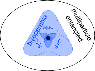
We consider for simplicity three parties, Alice (A), Bob (B) and Charlie (C), the generalization to more parties is straightforward. A three-particle state is fully separable and contains no entanglement, if it can be written as a mixture of product states
| (1) |
where the form a probability distribution. For states which are not of this form there are different types of entanglement. It may happen that the particles and are entangled, whereas particle is separable. Such a state is said to be separable with respect to the bipartition versus () and a mixture of product states of the joint system and is the single system ,
| (2) |
Similarly one defines states which are separable with respect to the other possible splittings and . The convex hull of these three sets defines the set of biseparable states,
| (3) |
States outside this set are called genuine multiparticle entangled and are the states of interest for many experimental applications.
In the three-particle case one ends up with a nested structure of different kinds of separable states, all of which are contained within the biseparable states (see Fig. 1(a)).
2.2 PPT mixtures and the genuine multiparticle negativity
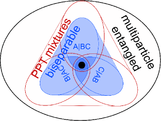
At present, there is no general framework to prove or disprove the existence of a biseparable decomposition for arbitrary mixed states. In Ref. [1] this problem was studied by introducing a relaxation. Instead of trying to characterize the set of biseparable states as given in Eq. (3) one characterizes the superset of so-called PPT mixtures.
The idea builds on the fact that the separable states are a subset of the states with a positive partial transpose (PPT states) [14]. Recall that a bipartite state
| (4) |
is called PPT, if its partial transposition with respect to the subsystem ,
| (5) |
has no negative eigenvalues.
In the three-particle case [see Fig. 1(b)] PPT mixtures are states, which can be written as
| (6) |
A general PPT mixture on more than three parties will have terms, one for each partition of the system into two parts. Such a bipartition is a splitting of the system into a part and its complement . Note, however, that and label the same bipartition.
The main advantage of this approach is that for any given multiparticle state one can directly check whether it is a PPT mixture or not. For that, it was shown that the non-existence of such a decomposition is equivalent to the existence of a fully decomposable witness detecting the state . Such a witness is an operator , which can be written for all possible bipartitions as , with positive operators and . Finding such a witness can be cast into a so-called semidefinite program (SDP, see also below), which can be solved efficiently with standard numerical routines [15, 16].
Building upon this idea, Ref. [1] introduced a computable entanglement monotone called the genuine multiparticle negativity (GMN). The basic idea is to take a fully decomposable witness as above, and use the violation of it as a quantifier of entanglement. More precisely, one defines the GMN via the optimization problem:
For the three-particle case the witness operator has to be decomposable into , and with . Since this measure is defined as an optimization over a set of witnesses it is closely related to the approach to quantify entanglement based on entanglement witnesses as in Ref. [18]. In contrast to the existing approaches, however, it can be directly computed using SDP [16], since the optimization problem in Eq. (2.2) is directly an optimization problem of this class. We finish this section by recalling the main properties of the GMN as proved in Refs. [1, 17]:
Lemma 1. The measure as defined by Eq. (2.2) satisfies:
-
1.
vanishes on all biseparable states , i.e. . Further, if is no PPT mixture, then .
-
2.
is non-increasing under full LOCC operations (no joint operations on more than one part are allowed), i.e. .
-
3.
is invariant under local basis changes , i.e. .
-
4.
is convex, i.e. holds for all convex decompositions .
-
5.
is bounded by , where is the lowest dimension of any particle in the system [17].
-
6.
If the system consists of two parties only, then equals the bipartite negativity [8].
3 The genuine multiparticle negativity as a convex roof measure
In this section we introduce a renormalized version the GMN by changing the normalization of the witness operator. Our main motivation is the following. So far, we have a good understanding of the GMN in terms of witnesses. In state space however, there is no satisfying interpretation. By slightly altering the definition the GMN has a direct simple interpretation in the witness and in the state space picture.
3.1 Modifying the definition of the genuine multiparticle negativity
For any state the renormalized GMN is given by
Compared to the original definition in Eq. (2.2), the only difference is a relaxation in the constraints on the positive operators , which is not bounded by anymore. Note that this definition was already used in Ref. [7] to quantify genuine multiparticle entanglement in a device independent manner.
The interesting point is that the renormalized GMN has an interpretation in state space as coming from an optimization over decompositions of the density matrix . This is known as the mixed convex roof construction [9], and many entanglement measures are defined via such an optimization. In the present case, one deals with a so-called mixed convex roof, and this can be derived from the the dual problem [15] to the semidefinite problem in Eq. (3.1). We have:
Theorem 2. Let be the bipartite negativity given by , where are the negative eigenvalues of . Then the genuine multiparticle negativity equals a mixed convex roof of bipartite negativities. That is
| (9) |
where the summation runs over all inequivalent partitions of the system and the minimization is performed over all mixed state decompositions of the state .
The proof of this Theorem can be found in A.
Note that the optimization in Eq. (9) can also be written in a different way: If one defines for an arbitrary multiparticle quantum state the quantitity as the bipartite negativity, minimized over all bipartitions, then the multiparticle negativity can be written as
| (10) |
where now the minimization is over all decompositions into mixed states and does not label the bipartitions anymore. In this way, the connection to the usual convex roof construction (see Ref. [19] and also Eq. (29) below) becomes more transparent. In general however mixed and pure state convex roofs are extremely difficult to compute. In this respect it is important to highlight that the renormalized GMN can be computed using SDP.
3.2 Comparison with the original definition of the GMN
First, we can state that all the properties of the GMN also hold for the renormalized definition and one additional property is new.
Lemma 3. For the multiparticle negativity as defined in Eq. (3.1) all the properties (i) to (vi) listed in Lemma 1 hold. Additionally, it has the following property:
-
7.
If is a pure state, then
(11) where the minimization is performed over all bipartite splittings of the system.
Proof. The first properties from Lemma 3 can be proved directly as in Lemma 1 by modification of the respective proofs in Ref. [1]. Concerning statement (vii), note that for a pure state there is only a single (and trivial) decomposition, namely
Note that due to property (ii) of Lemmata 1 and 3 both versions of the GMN are entanglement monotones. Naturally, the question arises how the renormalized GMN performs in detecting genuine multiparticle entangled states. If one is interested in the quantification of genuine multiparticle entanglement with the help of an entanglement monotone then either of the two monotones can be used as they are nonzero on the same set of states.111One can modify the original MATLAB implementation of the PPT mixer [16] to get an implementation of the renormalized GMN, by simply commenting line 90 in the “entmon.m” file. One directly has:
Corollary 4. For all , and .
Another feature of the renormalized GMN are the natural upper and lower bounds, arising from Eq. (3.1) and Eq. (9) in Theorem 2. First, as for the original GMN, every witness , which satisfies the constraints in Eq. (3.1) provides a lower bound on the renormalized genuine multiparticle negativity
| (12) |
Second, every mixed state decomposition of a state , , provides an upper bound on the renormalized GMN
| (13) |
This property makes the renormalized GMN easier to compute analytically. Note that the upper bounds of the renormalized GMN also provide upper bounds for since .
Finally, note that for pure states the renormalized GMN can directly be computed with the help of Lemma 3. Sometimes it coincides with the original GMN for pure states, and sometimes not. An example is the three-qubit GHZ state , where . On the other hand, for the three-qubit W state , and .
4 Analytic computation of the genuine multiparticle negativity
In this section we use our previous results to provide analytic formulae of the GMN for two important families of multi-qubit states. These are the -qubit GHZ-diagonal and four-qubit cluster-diagonal states. The idea in both cases is to construct for each family of states a family of witnesses lower bounding the GMN and a family of decompositions, which results in upper bounds. Since the bounds coincide and hold true for the original and the renormalized GMN they provide closed formulas for both monotones.
4.1 Graph states
Both state families are connected to so called graph states, which are relevant in many applications in quantum information processing [20]. One defines them as follows: consider a graph which is a set of vertices with edges connecting them (see Fig. 2), where each vertex corresponds to a qubit. For each vertex we define its neighbourhood by the set of all vertices, which are connected to . Denote by , and the Pauli matrices , and on the -th particle with the identity on all the other. Then we can define for each vertex a so-called stabilizing operator
| (14) |
The graph state is the unique -qubit eigenstate to eigenvalue to all .
| (15) |
One can extend this framework by considering all common eigenstates of the stabilizing operators. We label those different states by their eigenvalues of on the stabilizing operators , such that with . Note that these states are all orthogonal and thus form a basis in the -qubit Hilbert space, the so-called graph state basis. Mixed states, which are diagonal in the graph state basis are determined by their fidelities
| (16) |
They are called graph-diagonal and have the property that they are invariant under the group generated by the stabilizing operators, i.e. for all .
Note that an arbitrary state can be transformed into a graph-diagonal state by the symmetrization operation
| (17) |
were the summation runs over all group elements of the group generated by the . Since all consist of local Pauli operators only this symmetrization does not increase entanglement and hence .

4.2 -qubit GHZ-diagonal states
In this paragraph we consider generalized Greenberger-Horne-Zeilinger (GHZ) states. That are states, which are diagonal in the -qubit GHZ-basis consisting of states , where and . In the three-qubit case this basis consists of the states , , and . Note that these states are invariant under the group generated by and for . This group is local unitary equivalent to the group corresponding to the star graph as shown in Fig. 2, were each node is connected to node one.
A three-qubit state diagonal in the GHZ basis is of the form
| (18) |
with .222GHZ-diagonal states have real , but we stress that all of our results hold true for states with complex as well. A general -qubit GHZ-diagonal state would have the same shape, with independent real on the diagonal and corresponding real on the anti-diagonal. The eigenvalues of these states are , . Hence to be a valid density matrix one needs and for all .
We now make use of the special structure of this class of states to construct explicit upper and lower bounds, which are valid for both versions of the GMN.
Lemma 5. For all GHZ-diagonal -qubit states
| (19) |
where and denotes the fidelity with the GHZ-basis state . also holds for the slightly more general case with complex on the anti-diagonal.
Proof. We will prove the statement for the three-qubit case, a generalization is straightforward. First, consider the case where the right-hand-side of Eq. (19) is nonzero. Without loss of generality one can assume that the maximum is achieved for and thus we have . Let for , then and
| (20) |
¿From the positivity of it follows that and so
| (21) |
Using these weights one decomposes into a convex combination with
| (22) |
| (23) |
| (24) |
and .
To calculate the upper bound resulting from this decomposition we first have to compute the action of partial transposition with respect to subsystem , and on three-qubit GHZ-diagonal state. One directly sees that the partial transposition permutes the anti-diagonal elements. In the three-qubit case transposition of the first qubit exchanges , and the corresponding conjugate pairs. The partial transposition of the second qubit exchanges , and conjugate pairs and the partial transposition on the last qubit exchanges , and conjugate pairs. So has the following four non-zero eigenvalues
| (25) |
Taking into account Eqs. (20) and (21) the only non positive eigenvalue is and thus . This results in the conjectured upper bound
| (26) |
This bound can be rewritten as , since . If we then use the fidelities and with and , then for real , which proves the alternative expression in Eq. (19).
If, on the other hand, the right-hand-side of Eq. (19) is zero, then , which is known to be a necessary and sufficient criterion for biseparability [21] and for all biseparable states , .
Lemma 6. Consider a -qubit GHZ-diagonal state then there exists a fully decomposable witness satisfying the properties in Eq. (3.1), such that
| (27) |
where . also holds for the slightly more general case with complex on the antidiagonal.
Proof. As in the last proof we consider the three-qubit case. Without loss of generality the minimum in inequality (27) is achieved for . Then the position of in in the computational basis is given by the tuple . From this tuple we construct the witness , with . In the more general case, where the one would insert an additional phase in front of .
The witness is of the form of as in Eq. (18). From the discussion in the proof of Lemma 5 it follows that . Hence, is fully decomposable with and . In case the minimum equals zero the witness is given by , and . This proves the claim.
In summary, we have:
Corollary 7. For all GHZ-diagonal -qubit states
| (28) |
where denotes the fidelity with the GHZ-basis state . holds also true for the slightly more general case with complex on the anti-diagonal.
Three remarks are in order at this point. First, for general states the right hand side of Eq. (28) still gives a lower bound on the renormalized GMN since every state can be transformed into a GHZ-diagonal by means of local operations only. Thus the analytic expression in Eq. (28) might be used to estimate genuine multiparticle entanglement also for a general state. Second, we calculated the value for the renormalized GMN as defined in Eq. (3.1), but the same result holds for the GMN according to Eq. (2.2). This is because the witness constructed in the proof of Lemma 6 fulfils also the conditions of Eq. (2.2) and Lemma 5 delivers an upper bound due to Corollary 4. Third, note that the analytic formula we found coincides with the maximal violation of the biseparability criteria derived in Ref. [21].
Further, it is interesting to compare our expression for the GMN to the analytic formula of the genuine multiparticle concurrence (GME-concurrence) [11] for GHZ-diagonal -qubit states [10]. The GME-concurrence is defined as follows: For a bipartite pure state the concurrence is given by where is the reduced state on Alice’s system. For a pure multipartite state , the genuine multiparticle concurrence is defined as the minimum of the bipartite concurrences , minimized over all bipartitions. Finally, for mixed states the measure is given by the convex roof construction
| (29) |
Note that contrary to the mixed convex roof optimization in Eq. (9) here only pure state decompositions are involved. This pure state convex roof, however, is in general nearly impossible to compute and therefore one relies on lower bounds for practical applications.
The GME-concurrence has been computed for GHZ-diagonal states [10] and one observes that up to a factor of two both expressions coincide. There are, however, deeper connections: for a pure multiqubit state one has
| (30) |
This follows directly from known relations between the bipartite negativity and the bipartite concurrence [22]. Since the GMN can be defined via the mixed convex roof, which is an optimization over a larger set than the pure convex roof of the GME-concurrence, the general bound
| (31) |
holds for all mixed states. Therefore, Theorem 2 provides a way to obtain lower bounds on the GME-concurrence via semidefinite programming or analytical calculations. We will see in the next section, that the value of the is much more sensitive to entanglement than the known lower bounds on the GME-concurrence.
4.3 Four-qubit cluster-diagonal states
In this section we consider the linear graph having four vertices as shown in Fig. 2. The corresponding stabilizing operators as defined in Eq. (14) are given by
| (32) |
As already discussed, the corresponding graph state basis is given by , , , . We will also write this states as , with and denote by the complement of . Then we consider the graph-diagonal state
| (33) |
and wish to compute the GMN for these states. Note that in the literature the four-qubit cluster state is often defined via the local unitary equivalent stabilizing operators , , and . Then the corresponding eigenstate to eigenvalue on all is the familiar cluster state
| (34) |
in the computational basis.
For discussing genuine multiparticle entanglement of cluster diagonal states, the following two classes of witnesses
| (35) | |||
| (36) |
have turned our to be useful. It has been shown that these witnesses provide necessary and sufficient criteria to detect genuinely multiparticle entanglement in these states [23]. Based on these, Chen et al. [24] provided a closed formula for the genuine multiparticle relative entropy of entanglement as entanglement monotone. Here we provide a closed formula for the GMN for four-qubit cluster-diagonal states.
In terms of the fidelity the expectation values of the witnesses in Eqs. (35) and (36) read
| (37) |
First we note that all of these witnesses can be used to bound the GMN from below:
Lemma 8. For all partitions of the four partied system there exists , such that
| and | (38) |
Proof. One can easily compute the eigenvalues of and for all to be and . For any other witness () there exists a local unitary transformations, such that () transforms into it.
Taking into account that each of the above witnesses gives a lower bound on the GMN [see Eq. (12)] we have that
| (39) |
for all four-qubit cluster-diagonal states. As done for the GHZ-diagonal states we can use specific decompositions [see Eq. (9)] to construct upper bounds on the GMN, which result in an analytic formula for all four-qubit cluster states.
Theorem 9. Let be diagonal in the cluster graph basis, then the GMN of that state is given by
| (40) |
This means that effectively the largest violation of the witnesses in Eqs. (35) and (36) gives the value of the GMN.
The proof of this Theorem is given in B.
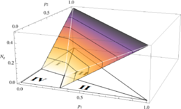
Let us discuss some examples. For the graph state mixed with white noise we obtain , which gives the exact threshold for genuine multiparticle entanglement [23]. In Fig. 3 a two-parameter family is shown, which is is genuine multiparticle entangled in three regions and biseparable in one. In each of the regions a different optimal witness gives the GMN.
Finally, we compare our results to computable lower bounds on the GME-concurrence introduced in Refs. [11, 13] and general lower bounds on the linear entropy based genuine multiparticle entanglement measure in Ref. [12]. To compare the performance we calculate the value down to which is still detected as genuine multiparticle entangled. Using the general bound of the GME-concurrence in Ref. [11] we found that even the pure four-qubit cluster-diagonal state is not detected. Using instead a set of inequalities build to detect genuine multiparticle entanglement in -qubit Dicke states [13] we found to be detected for .333Note that we applied local filters to the state to enhance its detectability, where is a normalization and the are linear maps on the single qubit systems. A better detection was achieved with the general lower bound on the genuine multiparticle entanglement measure given by Theorem 1 from Ref. [12]. We found that the state was detected as genuine multiparticle entangled for , which is closer to the exact threshold but not the exact value. We can therefore conclude that although the analytic formula for the GME-concurrence is equivalent to ours for -qubit GHZ-diagonal states, the lower bounds for four-qubit cluster-diagonal states do not match our analytic results.
5 Conclusions
In conclusion we have shown that the renormalized genuine multiparticle negativity can be expressed in two equivalent ways: As an optimization over suitable normalized fully decomposable witnesses as given by Eq. (3.1) and as mixed convex roof of the minimal bipartite negativity as given by Eq. (9). As a direct consequence of these equivalent definitions there are naturally arising lower and upper bounds, which we used to obtain an exact algebraic prescription of the genuine multiparticle negativity for the -qubit GHZ-diagonal and four-qubit cluster-diagonal states. These analytic expressions can also be used to obtain lower bounds on the genuine multiparticle negativity for arbitrary -qubit states.
There are several questions arising, which one might investigate in the future. First, since the scheme to obtain the analytic expression is quite general it should be possible to find closed expressions for other highly symmetric state families like other graph-diagonal states [20] or states with symmetry [25].
Second, it would be desirable to obtain an operational interpretation for the genuine multiparticle negativity. As the bipartite logarithmic negativity is the upper bound for distillable entanglement [8] one may speculate that our monotone is connected to the distillation rate of genuine multiparticle entangled states. Also, the multiparticle negativity may be related to different entanglement classes in the multiparticle case and the dimensionality of multiparticle entanglement [26].
Finally, recall that the shareability of quantum correlations among many parties is limited and these restrictions are known as monogamy relations [27, 28, 29]. For example, for a three-qubit system the bipartite entanglement of the splitting as measured by the concurrence is given by the entanglement in the reduced marginals plus the three tangle as a genuine tripartite contribution, [27]. It would be very interesting to derive similar relations for the genuine multiparticle negativity.
Appendix A Proof of Theorem 2
To start, we recall some notions of semidefinite programing [15]. The primal problem of an SDP reads
| (41) | |||||
| s.t. |
where and . The scalar product is the linear function to minimize and the linear matrix inequality , understood in terms of positive semi-definiteness holds all the constraints of the optimization. The dual problem to this primal problem is given by
| (42) | |||||
| s.t. | |||||
A point or is called feasible if it meets the constraints of the primal or dual respectively and . For any pair of feasible points both problems are connected to each other via . Moreover, if at least one of the problems is strictly feasible, i.e. that either a primal point satisfying or a dual point satisfying and exists, Theorem 3.1 in Ref. [15] ensures that both problems yield the same optimum .
The idea of the proof goes as follows. Using our renormalized GMN as given by Eq. (3.1) as the primal problem of a SDP we show that the corresponding dual problem is given by the left-hand-side of Eq. (9). Equality then follows by showing strict feasibility of the primal problem. We start the proof by rewriting the semidefinite program (3.1) as
| (43) | |||||
| s.t. | |||||
For the sake of readability we write down the proof by assuming a quantum system composed of three parts , and . A generalization to larger particle numbers is straightforward.
We choose a Hermitian operator basis , , such that . In this basis , and for . We gather the components of this decompositions in the vectors
| (44) |
where are the coefficients of , are the coefficients of and as well as the characterize parts of the optimization goal. If we merge these vectors into
| (45) |
we can rewrite the SDP (43) as
| (46) | |||||
| s.t. |
where has the following block diagonal form
| (47) | |||||
Here the vertical lines “” are introduced for notational convenience in order to to split the block diagonal matrix into three parts, each of which consists of three sub blocks. The first represents the constraint , the second ensures (equivalent to ) and the last one bounds (equivalent to ) for all . According to , we have:
| (48) |
The dual problem as given in Eq. (42) involves the calculation of and . To do so we can make use of the block-diagonal structure of the and write the corresponding diagonal blocks of into a new block-diagonal matrix
| (49) |
Note that the positivity of ensures the positivity of each block in . On the other hand if the blocks in are positive so is . We can now evaluate to write down the dual objective
| (50) |
The constraints can be evaluated similarly and split up into two types and . In detail, they read
| (51) | |||||
| (52) |
with . If we multiply Eq. (52) by and sum over all it immediately follows that
| (53) |
Eq. (51) multiplied by and summed over together with Eq. (53) yields
| (54) |
Actually, the dual problem optimizes in state space, which can be made apparent by introducing the following notation. Let and , then the constraint given by Eq. (54) corresponds to an optimization over all possible convex combinations of mixed quantum states . By introducing the constraint given by Eq. (53) can be rewritten as . The dual problem is then given by
| s.t. | (55) | ||||
which means that given a density matrix one minimizes over all decompositions and respective splittings of the partial transposition into a difference of two positive semidefinite operators .
Note that one can split this optimization into two steps. First, one has to optimize over all mixed state decompositions of , where each term in the decomposition is assigned to a certain bipartition. For a fixed decomposition one still has to minimize over with . This can be decomposed into the separate minimization of each over . If one compares these single optimizations to the bipartite negativity [8] of the respective partition
| (56) |
then . Hence we can rewrite the dual problem as given in Eq. (55) by
| s.t. |
Here we replaced the infimum by a minimum, since one optimizes a continuous function over a closed and bounded set.
To finish this proof we still have to show that the primal problem is strictly feasible such that both problems have the same optimal value. We find that with is a strictly feasible point for the primal problem given by Eq. (3.1). Hence, the genuine multiparticle negativity equals the dual optimization problem
| (57) |
Appendix B Proof of Theorem 9
Within this proof we will shorten the Dirac notation by setting . First, recall that a four-qubit cluster-diagonal state is biseparable, iff the following inequalities are satisfied [23]:
| (58) | ||||
| (59) |
Furthermore, Lemma 2 in Ref. [23] states that the density matrix
| (60) |
is biseparable, unless and both hold at the same time.
We now prove that the maximal violation of the relations (58) and (59) [this corresponds to the negative of the expectation values of some witness in Eqs. (37)] is an upper bound on the GMN. There are three cases:
Case one: None of the inequalities (58) and (59) is violated. In this case we already know that the state is biseparable [23] and hence , which coincides with the right-hand-side of (40) in this case.
Case two: The largest violation occurs in inequality (58). We can assume that it occurs for , for other indices the reasoning is similar. Using and the fact that all other inequalities are less violated we obtain
| (61) |
for arbitrary. Adding on both sides yields
| (62) |
Now consider the state . One can check that does not violate any of the inequalities (58) and (59), so it is biseparable. We choose , which is two times the violation of inequality (58). Then we can decompose into a genuine multiparticle entangled part with weight and a biseparable rest. This rest consists of a convex combination of biseparable states as in Eq. (60) and the biseparable state
| (63) |
Since only the first part is not biseparable and the GMN is convex , we obtain
| (64) |
which corresponds to the right-hand side of Eq. (40) in this case.
Case three: The largest violation occurs in Eq. (59). Without loss of generality for and . Relating the inequalities (58) and (59) with each other as in the second case we obtain
| and | (65) |
As a direct consequence we can split each of and into two non negative parts
| and | (66) |
With this definition of and we can write
| (67) |
where the state
| (68) | |||||
is biseparable. With these replacements the largest violation of inequality (59) is given by
| (69) |
One can decompose and further into two non negative parts
| and | (70) |
such that
| (71) |
Using this decomposition of the coefficients one can write as a convex combination of biseparable states of the form in Eq. (60). We can then split into a genuinely multiparticle entangled part and a biseparable rest
| (72) |
In this case this yields the last expected estimate on the GMN
| (73) |
So the maximal violation of the negative expectation values of the witnesses from Eqs. (35) and (36) gives upper bounds on the GMN, which proves the claim. As in the case of GHZ-diagonal states, the bound holds for both possible normalizations of the GMN.
References
References
- [1] B. Jungnitsch, T. Moroder and O. Gühne, Phys. Rev. Lett. 106, 190502 (2011).
- [2] E. Lötstedt and U. D. Jentschura, Phys. Rev. Lett. 108, 233201 (2012); E. Lötstedt and U. D. Jentschura, Phys. Rev. A 87, 033401 (2013).
- [3] M. Hofmann, A. Osterloh and O. Gühne, Phys. Rev. B 89, 134101 (2014).
- [4] S. N. Filippov A. A. Melnikov and M. Ziman, Phys. Rev. A 88, 062328 (2013).
- [5] M. Ali and O. Gühne, J. Phys. B: At. Mol. Opt. Phys. 47, 055503 (2014).
- [6] K. Stannigel, P. Rabl and P. Zoller New J. Phys. 14, 063014 (2012).
- [7] T. Moroder, J.-D. Bancal, Y.-C. Liang, M. Hofmann, and O. Gühne, Phys. Rev. Lett. 111, 030501 (2013).
- [8] K. Życzkowski, P. Horodecki, A. Sanpera and M. Lewenstein, Phys. Rev. A 58, 883 (1998); G. Vidal, R.F. Werner, Phys. Rev. A 65, 1 (2002).
- [9] D. Yang, M. Horodecki, R. Horodecki and B. Synak-Radtke, Phys. Rev. Lett. 95, 190501 (2005); B. Synak-Radtke and M. Horodecki, J. Phys. A: Math. Gen. 39, L423-L437 (2006); G. A. Paz-Silva and J. H. Reina, J. Phys. A: Math. Theor. 42, 055306 (2009); D. Yang, K. Horodecki, M. Horodecki, P. Horodecki, J. Oppenheim and W. Song, IEEE Trans. Inf. Theory 55, 3375 (2009).
- [10] S. M. Hashemi Rafsanjani, M. Huber, C. J. Broadbent and J. H. Eberly, Phys. Rev. A 86, 062303 (2012).
- [11] Z. Ma, Z. Chen, J. Chen, C. Spengler, A. Gabriel and M. Huber, Phys. Rev. A 83, 062325 (2011).
- [12] J. Wu, H. Kampermann, D. Bruß, C. Klöckl and M. Huber, Phys. Rev. A 86, 022319 (2012).
- [13] M. Huber, P. Erker, H. Schimpf, A. Gabriel, and B. Hiesmayr, Phys. Rev. A 83, 040301 (2011).
- [14] A. Peres, Phys. Rev. Lett. 77, 1413 (1996).
- [15] L. Vandenberghe and S. Boyd, SIAM Review 38, 49 (1996).
- [16] See the program PPTmixer, available at www.mathworks.com/matlabcentral/ fileexchange/30968.
- [17] B. Jungnitsch, T. Moroder, and O. Gühne Phys. Rev. A 84, 032310 (2011).
- [18] F. G. S. L. Brandão, Phys. Rev. A 72, 022310 (2005).
- [19] A. Uhlmann, Open Syst. Inf. Dyn. 5, 209 (1998).
- [20] M. Hein, W. Dür, J. Eisert, R. Raussendorf, M. Van den Nest and H.-J. Briegel, Quantum Computers, Algorithms and Chaos (Proc. Int. School of Physics ‘Enrico Fermi’) 162 (2006), Amsterdam: IOS Press; arXiv:quant-ph/0602096.
- [21] O. Gühne and M. Seevinck, New. J. Phys. 12, 053002 (2010).
- [22] K. Chen, S. Albeverio, S.-M. Fei, Phys. Rev. Lett. 95, 040504 (2005).
- [23] O. Gühne, B. Jungnitsch, T. Moroder, and Y.S. Weinstein, Phys. Rev. A 84, 052319 (2011).
- [24] X. Chen, P. Yu, L. Jiang and M. Tian, Phys. Rev. A 87, 012322 (2013).
- [25] T. Eggeling and R. F. Werner, Phys. Rev. A 63, 042111 (2001).
- [26] M. Huber and J.I. de Vicente, Phys. Rev. Lett. 110, 030501 (2013); C. Eltschka and J. Siewert Phys. Rev. Lett. 111, 100503 (2013).
- [27] V. Coffman, J. Kundu, and W. K. Wootters, Phys. Rev. A 61, 052306 (2000).
- [28] M. Koashi and A. Winter, Phys. Rev. A 69, 022309 (2004); T. J. Osborne and F. Verstraete, Phys. Rev. Lett. 96, 220503 (2006).
- [29] H. He, G. Vidal arXiv:1401.5843.