Normal A0–A1 stars with low rotational velocities ^,

Abstract

Context. The study of rotational velocity distributions for normal stars requires an accurate spectral characterization of the objects in order to avoid polluting the results with undetected binary or peculiar stars. This piece of information is a key issue in the understanding of the link between rotation and the presence of chemical peculiarities.

Aims. A sample of 47 low $v\sin i$ A0–A1 stars ($v\sin i<65$$\mbox{km}\,\mbox{s}^{-1}$), initially selected as main-sequence normal stars, are investigated with high-resolution and high signal-to-noise spectroscopic data. The aim is to detect spectroscopic binaries and chemically peculiar stars, and eventually establish a list of confirmed normal stars.

Methods. A detailed abundance analysis and spectral synthesis is performed to derive abundances for 14 chemical species. A hierarchical classification, taking measurement errors into account, is applied to the abundance space and splits the sample into two different groups, identified as the chemically peculiar stars and the normal stars.

Results. We show that about one third of the sample is actually composed of spectroscopic binaries (12 double-lined and five single-lined spectroscopic binaries). The hierarchical classification breaks down the remaining sample into 13 chemically peculiar stars (or uncertain) and 17 normal stars.

1 Introduction

Observations strongly suggested in the 1960s and 1970s that slow rotation is a necessary condition for the presence of peculiarities in the spectra of A-type stars (Preston, 1974, and references therein). Since then, the equatorial velocity below which chemically peculiar (hereafter CP) stars are observed is found to be around 120 $\mbox{km}\,\mbox{s}^{-1}$ (Abt & Moyd, 1973; Abt & Morrell, 1995). This observation is supported by theory that links the chemical peculiarities to the diffusion mechanism, occurring when the He ii convection zone disappears at equatorial velocities lower than 70–120 $\mbox{km}\,\mbox{s}^{-1}$ (Michaud, 1982). Atomic diffusion, under the competitive action of gravitational settling and radiative accelerations, alters the chemical abundances in stellar atmospheres, when mixing motions are weak. In theory, slow rotation should be a sufficient condition for the CP phenomenon to appear and Michaud (1980) wondered why a slowly rotating star would be non-peculiar.

The observational evidence that slow rotation is a sufficient condition for the presence of chemical peculiarities is not as straightforward. Whereas the dichotomy between normal and CP stars according to rotation rate is rather clear and unanimous in the literature for mid to late A-type stars (Abt & Moyd, 1973; Abt & Morrell, 1995; Royer et al., 2007), this is not the case for early A-type stars, from A0 to A3.

For Abt & Morrell (1995, hereafter AM), the bimodal shape of the equatorial velocity distribution can be explained by the different rotation rate of normal stars (fast) compared to peculiar and binary stars (slow). They conclude that the observed overlap between both distribution modes for A0–A1 stars is due to the inability to detect marginal CP stars or to evolutionary effects: rotation alone could thus explain the normal or peculiar appearance of an A star’s spectrum (Abt, 2000; Adelman, 2004). However, authors focusing on the rotational velocities of normal stars confirm the excess of slow rotators for normal A0–A1 stars (Dworetsky, 1974; Ramella et al., 1989; Royer et al., 2007), when removing known CP and binary stars. This excess of slow rotators is moreover observed at higher masses (Zorec & Royer, 2012).

The nature of these objects remains unclear. There is no doubt that a fraction of them is composed of so far unidentified spectroscopic binaries and/or CP stars; just how many genuine normal stars are slow rotators seems very much open again. Are slowly rotating normal A stars young objects that will become Ap stars and do not show chemical peculiarity yet, as suggested by Abt (2009)? Since the spectroscopic measurement of rotational velocity ($v\sin i$) is a projection on the line-of-sight, are low $v\sin i$ normal abundance A stars likely to be fast rotators seen at low inclination angle, such as Vega (Gulliver et al., 1994; Hill et al., 2010)? To answer these questions, the low $v\sin i$ A0–A1 normal stars from Royer et al. (2007, hereafter RZG) need to be investigated with new high-resolution and high signal-to-noise spectroscopic data. The purpose of this article is to perform a detailed abundance analysis and spectral synthesis to detect potential binary or CP stars and provide a list of confirmed normal low $v\sin i$ A0–A1 stars. The resulting subsample will be analyzed in greater depth in a following article.

This paper is organized as follows: the sample, its selection and the spectroscopic observations are described in Sect. 2. Section 3 deals with the determination of radial velocities and gives a list of suspected binaries. The atmospheric parameters and rotational velocities are respectively derived in Sect. 4 and Sect. 5. Section 6 presents the determination of abundance patterns and Sect. 7 details the classification based on these chemical abundances. The abundance patterns and the rotational velocity distribution are discussed in Sect. 8 and the results are summarized in Sect. 9. Comments on individual stars are given in Appendix A.

2 Data sample

2.1 Target selection

RZG built a sample of main-sequence A-type stars with homogenized $v\sin i$ using values from AM and Royer et al. (2002a, b). Chemically peculiar stars were removed on the basis of the spectral classification and the catalog of Renson et al. (1991). Binary stars were discarded on the basis of HIPPARCOS data (ESA, 1997) and the catalog of spectroscopic binaries from Pédoussaut et al. (1985). For A0–A1 stars, these criteria reduced the size of the original sample by about one third.

This paper focuses on a subsample of the A0–A1 normal stars, selected on their low $v\sin i$ ($\leq 65$ $\mbox{km}\,\mbox{s}^{-1}$), in order to investigate the slow rotator part of the distribution and accurately check whether these stars are normal or harbor signatures of multiplicity and/or chemical peculiarity. Using this criterion, 73 stars are selected on the whole sky. Among them, 47 can be observed from Observatoire de Haute-Provence (OHP). Table LABEL:tabstars, available online, lists the 47 targets defining our sample, together with their spectral type, $V$ magnitude, $v\sin i$ (Royer et al., 2002b) and the different parameters derived in the next sections.

Table 1: List of the 47 targets, with their derived parameters: rotational velocities, microturbulent velocity $\xi_{\mathrm{t}}$, effective temperature, gravity, luminosity and limb-darkening coefficient $\epsilon$ in the $B$ band.

HD	SpType	$V$	$v\sin i$			$\xi_{\mathrm{t}}$	$T_{\mathrm{eff}}$	$\log g$	$\log L/L_{\odot}$	$\epsilon$
		(mag)	($\mbox{km}\,\mbox{s}^{-1}$)			($\mbox{km}\,\mbox{s}^{-1}$)	(K)
			rgbgz	synth	ft
1439	A0IV	5.875	39	43.0	$45.3{\scriptstyle\pm 1.5}$	1.0	9640	3.75	$2.08{\scriptstyle\pm 0.04}$	0.6145
1561	A0Vs	6.538	60	63.7	$66.2{\scriptstyle\pm 1.4}$	1.3	8860	3.35	$1.91{\scriptstyle\pm 0.07}$	0.6580
6530	A1V	5.578	51	48.8	$103.1{\scriptstyle\pm 3.0}$	1.6	9500	3.87	$2.25{\scriptstyle\pm 0.04}$	0.6191
20149	A1Vs	5.606	23	21.8	$21.9{\scriptstyle\pm 1.0}$	1.0	9640	4.04	$2.15{\scriptstyle\pm 0.06}$	0.6113
21050	A1V	6.070	27	26.5	$27.8{\scriptstyle\pm 0.9}$	1.4	10420	4.30	$1.62{\scriptstyle\pm 0.03}$	0.5781
25175	A0V	6.311	55	55.0	$56.7{\scriptstyle\pm 1.5}$	1.5	9920	3.75	$2.09{\scriptstyle\pm 0.07}$	0.6031
28780	A1V	5.908	28	31.0	$33.0{\scriptstyle\pm 0.7}$	1.7	9640	3.86	$1.88{\scriptstyle\pm 0.05}$	0.6135
30085	A0IV	6.345	26	23.0	$24.2{\scriptstyle\pm 0.6}$	0.5	11300	3.95	$2.28{\scriptstyle\pm 0.07}$	0.5516
33654	A0V	6.156	60	72.0	$73.0{\scriptstyle\pm 4.1}$	3.3	9220	2.90	$3.63{\scriptstyle\pm 0.84}$	0.6389
39985	A0IV	5.971	28	28.5	$28.2{\scriptstyle\pm 1.2}$	0.6	10240	3.62	$1.83{\scriptstyle\pm 0.05}$	0.5917
40446	A1Vs	5.213	27	28.0	$23.6{\scriptstyle\pm 3.5}$	0.5	9550	3.95	$2.16{\scriptstyle\pm 0.10}$	0.6161
46642	A0Vs	6.46	49	57.0	$57.7{\scriptstyle\pm 1.4}$	2.3	9890	3.89	$1.57{\scriptstyle\pm 0.11}$	0.6028
47863	A1V	6.284	40	41.0	$47.1{\scriptstyle\pm 2.6}$	2.2	9520	3.45	$2.34{\scriptstyle\pm 0.10}$	0.6224
50931	A0V	6.274	65	75.0	$84.0{\scriptstyle\pm 5.5}$	1.4	9440	4.13	$1.31{\scriptstyle\pm 0.03}$	0.6185
58142	A1V	4.614	19	19.0	$18.7{\scriptstyle\pm 0.4}$	1.7	9520	3.79	$1.97{\scriptstyle\pm 0.02}$	0.6193
65900	A1V	5.646	33	34.8	$36.4{\scriptstyle\pm 1.5}$	2.0	9600	4.01	$1.67{\scriptstyle\pm 0.04}$	0.6135
67959	A1V	6.217	18	16.7	$15.5{\scriptstyle\pm 0.5}$	2.0	9310	3.71	$2.03{\scriptstyle\pm 0.07}$	0.6296
72660	A1V	5.799	9	7.0	$6.5{\scriptstyle\pm 0.4}$	1.5	9640	4.03	$1.57{\scriptstyle\pm 0.03}$	0.6116
73316	A1V	6.542	33	32.8	$35.2{\scriptstyle\pm 1.1}$	2.0	9830	4.30	$1.49{\scriptstyle\pm 0.04}$	0.5994
83373	A1V	6.391	28	28.5	$29.8{\scriptstyle\pm 1.4}$	1.6	10200	4.10	$1.73{\scriptstyle\pm 0.05}$	0.5884
85504	A0Vs	6.02	27	25.7	$27.6{\scriptstyle\pm 2.2}$	1.6	10200	3.82	$2.26{\scriptstyle\pm 0.08}$	0.5915
89774	A1V	6.169	60	63.3	$65.5{\scriptstyle\pm 2.1}$	2.1	9630	3.90	$1.83{\scriptstyle\pm 0.04}$	0.6135
95418	A1V	2.346	46	45.7	$46.2{\scriptstyle\pm 1.2}$	2.2	9620	3.89	$1.82{\scriptstyle\pm 0.00}$	0.6140
101369	A0V	6.210	65	67.5	$70.0{\scriptstyle\pm 3.9}$	1.0	9700	3.82	$1.97{\scriptstyle\pm 0.11}$	0.6112
104181	A1V	5.357	44	59.0	$55.5{\scriptstyle\pm 1.6}$	1.0	9660	4.00	$1.79{\scriptstyle\pm 0.02}$	0.6110
107655	A0V	6.176	46	45.0	$47.2{\scriptstyle\pm 1.4}$	2.0	9680	4.10	$1.53{\scriptstyle\pm 0.04}$	0.6088
119537	A1V	6.502	13	16.7	$13.3{\scriptstyle\pm 0.7}$	2.3	9260	4.14	$1.54{\scriptstyle\pm 0.04}$	0.6269
127304	A0Vs	6.055	14	8.9	$7.7{\scriptstyle\pm 0.6}$	1.5	10050	4.11	$1.70{\scriptstyle\pm 0.04}$	0.5939
132145	A1V	6.506	15	13.5	$12.7{\scriptstyle\pm 0.6}$	1.7	9680	4.25	$1.59{\scriptstyle\pm 0.05}$	0.6063
133962	A1V	5.581	49	52.3	$54.8{\scriptstyle\pm 1.6}$	1.2	10130	4.32	$1.66{\scriptstyle\pm 0.02}$	0.5882
145647	A0V	6.092	43	44.0	$47.2{\scriptstyle\pm 1.3}$	0.5	9560	3.95	$1.72{\scriptstyle\pm 0.05}$	0.6159
145788	A1V	6.255	16	13.0	$9.8{\scriptstyle\pm 0.8}$	2.3	9410	3.73	$1.88{\scriptstyle\pm 0.08}$	0.6250
154228	A1V	5.918	42	44.8	$45.2{\scriptstyle\pm 1.2}$	2.2	9750	4.20	$1.40{\scriptstyle\pm 0.02}$	0.6042
156653	A1V	6.002	43	43.6	$45.3{\scriptstyle\pm 2.0}$	2.3	9270	3.69	$1.82{\scriptstyle\pm 0.08}$	0.6320
158716	A1V	6.464	15	8.0	$6.4{\scriptstyle\pm 0.8}$	2.8	9300	4.39	$1.19{\scriptstyle\pm 0.03}$	0.6215
172167	A0V	0.03	24	23.5	$24.5{\scriptstyle\pm 1.4}$	1.0	9550	4.05	$1.73{\scriptstyle\pm 0.00}$	0.6149
174567	A0Vs	6.634	15	13.0	$10.5{\scriptstyle\pm 0.9}$	1.0	9710	3.59	$2.23{\scriptstyle\pm 0.10}$	0.6131
176984	A1V	5.42	23	30.0	$29.6{\scriptstyle\pm 1.0}$	2.0	9680	3.44	$2.20{\scriptstyle\pm 0.04}$	0.6155
183534	A1V	5.75	49	53.0	$51.8{\scriptstyle\pm 5.8}$	0.2	9930	4.24	$1.79{\scriptstyle\pm 0.02}$	0.5966
196724	A0V	4.82	52	50.5	$51.6{\scriptstyle\pm 2.2}$	1.3	10400	4.18	$1.87{\scriptstyle\pm 0.06}$	0.5801
198552	A1Vs	6.618	52	51.6	$53.7{\scriptstyle\pm 1.1}$	3.0	9230	4.14	$1.39{\scriptstyle\pm 0.06}$	0.6284
199095	A0V	5.748	32	27.8	$27.8{\scriptstyle\pm 1.3}$	0.9	9920	4.05	$1.79{\scriptstyle\pm 0.02}$	0.5999
217186	A1V	6.342	60	64.0	$66.7{\scriptstyle\pm 2.0}$	1.9	9190	4.00	$1.29{\scriptstyle\pm 0.04}$	0.6330
219290	A0V	6.319	54	59.0	$61.4{\scriptstyle\pm 1.9}$	1.5	9790	4.15	$1.66{\scriptstyle\pm 0.04}$	0.6034
219485	A0V	5.886	23	27.0	$27.3{\scriptstyle\pm 0.8}$	1.2	9580	3.81	$1.91{\scriptstyle\pm 0.03}$	0.6165
223386	A0V	6.328	33	33.0	$36.8{\scriptstyle\pm 1.2}$	1.2	9890	4.11	$1.62{\scriptstyle\pm 0.07}$	0.6001
223855	A1V	6.292	60	62.0	$71.5{\scriptstyle\pm 4.6}$	1.3	9890	4.14	$1.70{\scriptstyle\pm 0.06}$	0.5999

2.2 Spectroscopic observations

Spectra of our targets were collected at OHP and observations were spread over an eight year period. The first two runs (April 2005 and June 2006) used the ÉLODIE spectrograph ($R\approx 42000$, Baranne et al. 1996). Then ÉLODIE was decommissioned in August 2006 and replaced with a more efficient instrument offering a higher spectral resolution: SOPHIE ($R\approx 75000$, Perruchot et al. 2008). The last part of our program used SOPHIE, in three different runs: July 2009, February 2011 and February 2012. Archival data have also been used: about half the ÉLODIE spectra were taken from the ÉLODIE archive (Moultaka et al., 2004) and spectra of Vega were taken from the SOPHIE archive. Table LABEL:indivspectra (available electronically) lists the different observations of our targets, indicates the corresponding instrument, the observation date, the number of co-added spectra, the modified Julian date at the center of the exposure(s), the signal-to-noise ratio (S/N) derived using the DER_SNR algorithm (Stoehr et al., 2008) and the measured radial velocity, corrected from the barycentric motion (see Sect. 3). The initial observational strategy was derived from the twofold goal of our program: (i) obtain good S/N spectra ($\approx 150$–200) to perform, using synthetic spectra at low $v\sin i$, a detailed abundance analysis of unblended weak lines, allowing us to identify the normal stars; (ii) focus on these stars and obtain high S/N spectra ($\approx 400$) to analyze the line profiles and search for gravity-darkening signatures.

2.3 Data reduction

For both ÉLODIE and SOPHIE, data are automatically reduced to produce 1D extracted and wavelength calibrated échelle orders. When stars are observed several times during one observation night, the corresponding spectra are coadded. Then, for each reduced spectrum, échelle orders are normalized separately, using a Chebychev polynomial fit with sigma clipping, rejecting points above 6-$\sigma$ or below 1-$\sigma$ of the continuum. Normalized orders are merged together, weighted by the blaze function and resampled in a constant wavelength step $\Delta\lambda=0.02$Å. Only the spectral intervals outside the wings of Balmer lines and the atmospheric telluric bands are finally retained: 4150–4300Å, 4400–4790Å, 4920–5850Å and 6000–6275Å.

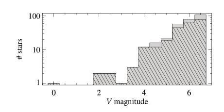
Figure 1: Counts in $V$ magnitude bins for northern ($\delta>-15\degr$) A0–A1 main sequence stars in the HIPPARCOS catalog (gray) and in the $v\sin i$ sample (hatched).

2.4 Completeness

Besides selections in $v\sin i$ and the absence of spectroscopic peculiarities, the aforedescribed sample is magnitude-limited and censored in declination and spectral type. These censorships can be applied to the HIPPARCOS catalog (ESA, 1997), complete down to $V=7.3$  (Perryman et al., 1997), to estimate the completeness of the sample. The selection criteria are the following:

• declination $\delta$ higher than $-15\degr$ to reproduce the observability bias due to the location of OHP (i.e. 63% of the celestial sphere),

• spectral class containing A0 or A1, and luminosity class either V, IV/V or IV, to reproduce the selection made in RZG,

• magnitude $V$ brighter than 6.65 .

This selection results in 303 stars from the HIPPARCOS catalog, among them 240 belong to the sample studied by RZG. The star counts per bin of $V$-magnitude are compared in Fig. 1. The ratio of these two counts gives a completeness of about 80%.

When limited to normal stars, using the results from RZG, 151 stars remain out of the 240. Our 47 targets correspond to the $v\sin i$-truncated subsample out of these 151 stars.

Table 2: List of observations and barycentric radial velocity measurements (RV) for the target sample. Asterisks, following the instrument name, indicate the spectra have been retrieved from the corresponding archive. Spectra observed the same night were combined into one spectrum. The number of input spectra, the modified Julian date (MJD) at the center of the exposure(s) and the combined signal-to-noise (S/N) are also given.

HD	Instrument	Date	#	MJD	S/N	RV
			spectra			($\mbox{km}\,\mbox{s}^{-1}$)
1439	SOPHIE	2009-08-05	1	55049.055625	213	$-9.57\pm 0.46$
	SOPHIE	2011-02-11	2	55603.765526	326	$-10.38\pm 0.48$
1561	SOPHIE	2009-08-05	1	55049.042685	210	$-18.44\pm 0.88$
	SOPHIE	2011-02-11	3	55603.792789	337	$-0.04\pm 0.92$
6530	SOPHIE	2009-08-05	3	55049.122963	387	$10.71\pm 2.75$
20149	ELODIE*	2004-01-02	1	53006.871601	106	$-9.01\pm 0.16$
	SOPHIE	2009-08-05	3	55049.086474	399	$-12.11\pm 0.16$
	SOPHIE	2011-02-11	2	55603.834201	356	$-12.32\pm 0.16$
	SOPHIE	2012-02-13	2	55970.794641	341	$-10.70\pm 0.16$
	SOPHIE	2012-02-14	2	55971.764421	370	$-10.88\pm 0.16$
21050	SOPHIE	2009-08-05	1	55049.104537	226	$-1.10\pm 0.23$
	SOPHIE	2011-02-11	2	55603.856759	69	$-1.08\pm 0.44$
	SOPHIE	2012-02-13	2	55970.773571	328	$-0.89\pm 0.24$
25175	SOPHIE	2011-02-11	1	55603.817766	222	$31.62\pm 0.76$
	SOPHIE	2012-02-13	3	55970.818221	308	$31.33\pm 0.73$
28780	SOPHIE	2012-02-13	2	55970.847066	340	$-14.19\pm 0.29$
30085	SOPHIE	2012-02-13	3	55970.874525	316	$8.27\pm 0.20$
33654	SOPHIE	2012-02-13	2	55970.904277	180	$-3.12\pm 1.10$
39985	ELODIE*	1995-12-20	1	50071.994159	138	$13.47\pm 0.24$
40446	ELODIE*	1999-12-20	1	51532.843002	160	$47.80\pm 0.20$
46642	ELODIE*	2003-01-15	1	52654.978756	190	$31.62\pm 0.81$
	SOPHIE	2012-02-14	3	55971.822326	332	$38.41\pm 0.78$
47863	SOPHIE	2012-02-14	3	55971.789437	365	$23.80\pm 0.52$
50931	SOPHIE	2012-02-14	3	55971.859687	345	$42.06\pm 1.46$
58142	ELODIE*	1998-01-28	1	50841.980507	172	$26.94\pm 0.12$
	ELODIE*	2004-01-03	1	53007.964181	300	$26.76\pm 0.12$
	ELODIE*	2005-02-02	1	53403.947654	270	$26.90\pm 0.12$
	ELODIE*	2005-02-03	1	53404.944216	292	$26.66\pm 0.12$
65900	ELODIE*	1995-12-21	1	50072.040836	107	$43.06\pm 0.36$
67959	ELODIE	2005-04-21	1	53481.846784	106	$23.74\pm 0.09$
72660	ELODIE*	1997-03-20	1	50527.808905	64	$3.22\pm 0.03$
	ELODIE*	2004-01-03	1	53007.074899	118	$4.28\pm 0.06$
	ELODIE*	2004-01-04	1	53009.017029	152	$4.68\pm 0.06$
	ELODIE*	2004-04-11	1	53106.829269	192	$4.74\pm 0.07$
73316	SOPHIE	2012-02-13	3	55970.946798	146	$27.68\pm 0.34$
	SOPHIE	2012-02-14	3	55971.894159	335	$28.02\pm 0.33$
83373	SOPHIE	2012-02-14	4	55971.999699	292	$26.58\pm 0.24$
85504	ELODIE*	1996-04-24	1	50197.825920	114	$103.76\pm 0.24$
	SOPHIE	2012-02-13	2	55971.001111	63	$104.03\pm 0.32$
	SOPHIE	2012-02-14	4	55971.960573	289	$103.70\pm 0.24$
89774	ELODIE	2005-04-22	1	53482.912204	102	$13.28\pm 0.94$
	SOPHIE	2012-02-14	3	55971.926975	293	$12.18\pm 0.85$
95418	ELODIE*	1997-02-20	1	50499.547959	170	$-13.52\pm 0.66$
	ELODIE*	2004-03-10	1	53074.002745	232	$-13.73\pm 0.50$
	ELODIE*	2005-02-04	1	53405.056783	283	$-13.89\pm 0.53$
	SOPHIE	2011-02-11	5	55604.191435	375	$-13.67\pm 0.51$
101369	ELODIE	2005-04-21	2	53481.910739	182	$7.70\pm 1.79$
104181	ELODIE*	2004-04-26	1	53121.940547	209	$-1.29\pm 0.84$
	SOPHIE	2012-02-14	3	55972.076979	299	$-0.34\pm 0.73$
107655	ELODIE*	2004-04-08	1	53103.058789	243	$-2.74\pm 0.59$
	SOPHIE	2012-02-14	3	55972.034603	338	$-3.49\pm 0.54$
119537	ELODIE	2006-06-02	1	53888.856696	105	$54.81\pm 0.08$
	SOPHIE	2012-02-14	7	55972.175921	254	$-62.46\pm 0.07$
127304	ELODIE	2005-04-21	1	53481.985365	223	$-22.30\pm 0.11$
132145	ELODIE	2005-04-22	2	53482.066887	219	$-9.98\pm 0.07$
	SOPHIE	2012-02-14	4	55972.113021	277	$-9.73\pm 0.07$
133962	ELODIE	2005-04-22	1	53482.131317	201	$-12.63\pm 0.73$
	SOPHIE	2011-02-11	2	55604.224086	215	$-13.29\pm 0.73$
	SOPHIE	2012-02-14	3	55972.058538	329	$-13.11\pm 0.72$
145647	ELODIE	2006-05-31	2	53886.908366	107	$-15.12\pm 0.85$
	ELODIE	2006-06-03	1	53889.067390	156	$-15.75\pm 0.58$
145788	ELODIE	2006-06-01	2	53887.968344	128	$-13.05\pm 0.05$
154228	ELODIE*	1999-06-05	1	51334.988236	163	$-31.10\pm 0.50$
	ELODIE*	1999-06-06	1	51335.970245	244	$-31.66\pm 0.47$
156653	ELODIE*	1996-04-26	1	50199.123847	113	$2.37\pm 0.47$
	SOPHIE	2009-08-05	3	55048.835204	294	$4.24\pm 0.46$
158716	ELODIE	2006-06-02	2	53888.924720	117	$-25.44\pm 0.03$
172167	ELODIE*	2004-02-28	1	53063.215076	266	$-13.91\pm 0.19$
	ELODIE*	2004-03-01	1	53065.215871	288	$-13.82\pm 0.20$
	ELODIE*	2004-03-27	1	53091.176158	275	$-13.99\pm 0.20$
	ELODIE*	2004-03-29	2	53093.148334	357	$-13.91\pm 0.19$
	ELODIE*	2004-08-30	2	53247.816155	378	$-13.68\pm 0.19$
	ELODIE*	2004-08-31	2	53248.796281	355	$-13.62\pm 0.19$
	ELODIE*	2004-09-23	2	53271.772018	317	$-13.77\pm 0.19$
	ELODIE*	2004-09-24	2	53272.771336	320	$-13.50\pm 0.19$
	ELODIE*	2004-09-25	2	53273.769548	347	$-13.60\pm 0.20$
	ELODIE*	2004-11-05	2	53314.738914	296	$-13.52\pm 0.19$
	ELODIE*	2004-11-06	1	53315.726548	246	$-13.86\pm 0.18$
	ELODIE*	2004-11-07	2	53316.740124	251	$-13.49\pm 0.20$
	ELODIE*	2004-11-09	1	53318.732878	152	$-14.01\pm 0.20$
	ELODIE*	2005-04-20	2	53480.107426	309	$-13.89\pm 0.19$
	ELODIE*	2005-05-24	2	53514.082351	301	$-13.79\pm 0.19$
	ELODIE*	2005-05-25	1	53515.036852	254	$-13.94\pm 0.20$
	SOPHIE*	2006-09-08	1	53987.400894	109	$-14.07\pm 0.21$
	SOPHIE*	2009-09-28	4	55102.762360	1055	$-13.81\pm 0.19$
	SOPHIE*	2009-09-29	1	55103.761169	467	$-13.81\pm 0.19$
	SOPHIE*	2009-09-30	1	55104.763217	422	$-13.72\pm 0.19$
	SOPHIE*	2009-10-06	1	55110.777199	386	$-13.69\pm 0.19$
	SOPHIE*	2009-10-07	2	55111.751158	443	$-13.76\pm 0.19$
	SOPHIE*	2009-10-08	1	55112.772696	438	$-13.68\pm 0.19$
	SOPHIE*	2009-10-09	1	55113.756793	405	$-13.66\pm 0.19$
	SOPHIE*	2009-10-10	3	55114.744915	571	$-13.71\pm 0.19$
	SOPHIE*	2009-10-11	1	55115.742314	300	$-13.83\pm 0.19$
174567	ELODIE	2006-05-31	2	53887.000591	119	$-14.18\pm 0.05$
	SOPHIE	2009-08-05	3	55048.871358	355	$-10.84\pm 0.05$
176984	ELODIE	2006-06-02	1	53888.998090	153	$-47.68\pm 0.29$
	SOPHIE	2009-08-05	3	55048.903823	402	$-43.75\pm 0.24$
183534	ELODIE	2006-06-01	1	53887.075317	148	$9.88\pm 0.63$
196724	ELODIE*	2004-11-12	1	53321.779634	301	$-21.97\pm 0.64$
	ELODIE	2006-06-02	1	53888.083812	156	$-18.31\pm 0.52$
198552	SOPHIE	2009-08-05	2	55048.952500	314	$5.47\pm 0.69$
199095	ELODIE*	2005-10-14	1	53657.768627	168	$-24.99\pm 0.21$
	SOPHIE	2009-08-05	3	55048.925880	325	$3.49\pm 0.23$
217186	SOPHIE	2009-08-05	3	55048.980456	287	$18.67\pm 1.34$
219290	SOPHIE	2009-08-05	2	55049.003953	253	$-16.88\pm 0.83$
219485	SOPHIE	2009-08-05	1	55049.016284	239	$-4.48\pm 0.21$
223386	SOPHIE	2009-08-05	1	55049.027685	235	$-18.57\pm 0.34$
223855	SOPHIE	2009-08-05	1	55049.067083	225	$3.68\pm 1.05$

Table 2: continued.

3 Radial velocities

The normalized spectra are cross-correlated with a synthetic template extracted from the POLLUX database (Palacios et al., 2010) corresponding to the parameters $T_{\mathrm{eff}}=9500$ K, $\log g=4$ and solar metallicity (computed with synspec48, Hubeny & Lanz, 1992), to compute the cross-correlation function (hereafter CCF). The radial velocity is derived from the parabolic fit of the upper part (10%) of the CCF and the values are given in Table LABEL:indivspectra. The error on the radial velocity is determined from the cross-correlation function using the formulation given by Zucker (2003) and assuming the parabolic fit of the CCF.

3.1 Combining ÉLODIE and SOPHIE

Fourteen of our targets have spectra collected with both ÉLODIE and SOPHIE. In order to combine the different velocities and detect possible variations, the radial velocity offset between both instruments has to be retrieved. Boisse et al. (2012) derive a relation giving this offset as a function of the $B-V$ color index for late-type stars (G to K). The offset $\Delta_{\mathrm{E-S}}$ ranges from 0 to $-0.25$ $\mbox{km}\,\mbox{s}^{-1}$ for these spectral types.

To constrain this offset for the considered spectral type, publicly available spectra of Vega (HD 172167) are retrieved from the ÉLODIE and SOPHIE archives (respectively 16 observations and 10, see Table LABEL:indivspectra), and radial velocities are derived the exact same way. The respective average velocities are: $-13.44\pm 0.05$ $\mbox{km}\,\mbox{s}^{-1}$ and $-13.46\pm 0.07$ $\mbox{km}\,\mbox{s}^{-1}$. The offset for the considered spectral type is then defined as the difference between these average velocities:

$$\Delta_{\mathrm{E-S}}(\mathrm{A0})=0.02\pm 0.09\,\mbox{km}\,\mbox{s}^{-1}.$$ (1)

This offset is not significantly different from zero, and we choose not to correct the derived radial velocities for our targets.

3.2 Suspected binaries

The suspicion of binarity from the CCF is raised by the variation of the radial velocity, when several observations are available, and/or by an asymmetric shape of individual CCF.

The variation is taken as significant when the ratio of the external error over the internal error is $E/I\gtrsim 2$ (Abt et al., 1972). The external error is chosen as the standard deviation of the measurements for the different available observations, and the internal error is the one estimated using the formulation from Zucker (2003), which increases with the rotational broadening. Table 3 lists the ten stars with $E/I>2$. The number of observations for a given star remains small, as a radial velocity follow-up was not intended. These stars are suspected single-lined spectroscopic binaries (SB1).

Table 3: List of targets showing a variation in their radial velocity measurements, with the number of observations ($N$), the average barycentric radial velocity $\langle$RV$\rangle$, the external error $E$ and the internal error $I$.

HD	$N$	$\langle$RV$\rangle$	$E$	$I$
		($\mbox{km}\,\mbox{s}^{-1}$)	($\mbox{km}\,\mbox{s}^{-1}$)	($\mbox{km}\,\mbox{s}^{-1}$)
1561	2	$-9.2$	13.01	0.64
20149	5	$-11.0$	1.33	0.20
46642	2	$35.0$	4.80	0.73
72660	4	$4.2$	0.70	0.03
119537	2	$-3.8$	82.92	0.46
156653	2	$3.3$	1.32	0.57
174567	2	$-12.5$	2.36	0.46
176984	2	$-45.7$	2.78	0.50
196724	2	$-20.1$	2.59	0.41
199095	2	$-10.8$	20.14	0.49

The stars that display an asymmetric CCF are shown in Fig. 2. For two of them, several observations are available, and a variable radial velocity is noticed. The objects are suspected to be double-lined spectroscopic binaries (SB2).

Details on them and comparison with literature data can be found in Appendix A.

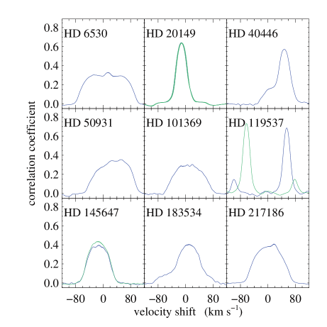
Figure 2: Cross-correlation functions of suspected binary stars from their asymmetric profiles. When available, several observations are overplotted. The velocity axis takes the barycentric correction into account.

4 Atmospheric parameters

We use the revised version of the uvbybeta code written by Napiwotzki et al. (1993) in order to derive effective temperatures ($T_{\mathrm{eff}}$) and surface gravities ($\log g$). The uvbybetanew relies on the calibration of the Strömgren photometry indices $uvby\beta$ in terms of $T_{\mathrm{eff}}$ and $\log g$. The photometric data are taken from Hauck & Mermilliod (1998). The derived fundamental parameters are displayed in Table LABEL:tabstars. According to Napiwotzki et al. (1993), errors on effective temperature are of the order of 2% for $T_{\mathrm{eff}}<10000$ K. The accuracy of surface gravity ranges from $\approx 0.1$ dex for early A-type stars to $\approx 0.25$ dex for hot B stars. In our study we fix the errors on $T_{\mathrm{eff}}$ and $\log g$ to be $\pm$125 K and $\pm$0.2 dex respectively.

A consistency check on $T_{\mathrm{eff}}$ and $\log g$ is performed by comparing the luminosity derived from the radius calibration (Torres et al., 2010), and the luminosity derived from HIPPARCOS parallaxes. Torres et al. (2010) give a polynomial expression of the stellar radius as a function of $T_{\mathrm{eff}}$, $\log g$ and [Fe/H] values. The luminosity is then derived from the Stefan-Boltzmann law. Absolute magnitudes are derived from the HIPPARCOS parallaxes (van Leeuwen, 2007) and from bolometric corrections in the $V$-band, interpolated in the tables from Bessell et al. (1998). The adopted bolometric luminosity parameter $\log L/L_{\odot}$, given in Table LABEL:tabstars, is derived by adopting $M^{\mathrm{bol}}_{\odot}=4.75\,$ (Allen, 1973). Figure 3 compares the luminosity values. The uncertainty from the calibrated luminosity is dominated by the $\log g$ uncertainty. In most cases the two agree to within the uncertainties, but a few outliers are present. These eight stars are indicated in Fig. 3 and seven out of them are suspected binaries from the previous section. The new outlier is HD 39985 (see Appendix A). In this plot, HD 33654 is out of range; the low gravity ($\log g=2.9$) derived from the photometry indicates a giant star, which is confirmed by the luminosity derived from the HIPPARCOS data: $\log L/L_{\odot}=3.63{\scriptstyle\pm 0.84}$, far brighter than the main-sequence. It is misclassified as a class V luminosity star.

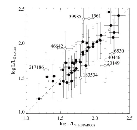
Figure 3: Consistency check using the luminosity derived from the Torres et al. (2010) calibration and the HIPPARCOS parallaxes. The dashed line is the one-to-one relation. The outliers are indicated by open symbols, together with their HD number.

At this point, the following stars are considered as SB2 with atmospheric parameters contaminated by their multiplicity (no abundances are derived): HD 1561, HD 6530, HD 20149, HD 39985, HD 40446, HD 46642, HD 50931, HD 101369, HD 119537, HD 145647, HD 183534, HD 217186. In addition, the following stars are considered as binaries without contamination of their atmospheric parameters: HD 72660, HD 156653, HD 174567, HD 176984, HD 196724. HD 199095. HD 33654 is also discarded from the sample as we focus on main-sequence stars.

Figure 4 shows the non-SB2 stars of the sample in the H-R diagram. Luminosities are derived from the trigonometric parallaxes.

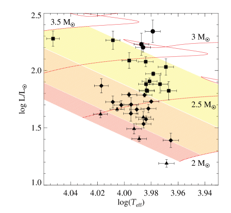
Figure 4: H-R diagram of the sample. Stars are plotted with different symbols according to their $\log g$, and the same limits are used to define regions from the model gravity: triangles for $4.2\leq\log g$ (red), diamonds for $3.95\leq\log g<4.2$ (orange), squares for $3.65\leq\log g<3.95$ (yellow) and circles for $\log g<3.65$. Evolutionary tracks from BaSTI (Pietrinferni et al., 2006), for $Z=0.0198$, with overshooting, are overplotted for the indicated stellar masses.

Evolutionary tracks from BaSTI (Pietrinferni et al., 2006) are computed with overshooting and for a solar metallicity of $Z=0.0198$. Considering the end of the main-sequence as its reddest point, just before the hook of the evolutionary track when the overall contraction starts, we chose three limits in $\log g$ plotted in Fig. 4. The first two limits in $\log g$ correspond to about one third and two thirds of lifetime on the main sequence for our mass range, according to BaSTI models. At the end of the main sequence the gravity given by BaSTI models is about $\log g=3.5$ for our mass range, and the last limit, $\log g=3.65$, corresponds to about 99% of the lifetime on the main sequence and defines a region that does not overlap with the hook in terms of gravity and position in the H-R diagram.

These fundamental parameters are used to calculate LTE model atmospheres using ATLAS9 (Kurucz, 1993). The ATLAS9 code assumes a plane-parallel geometry, a gas in hydrostatic and radiative equilibrium, and LTE. As explained in Gebran et al. (2008), ATLAS9 model atmospheres are calculated assuming Grevesse & Sauval (1998) solar abundances and using the prescriptions given by Smalley (2004) for convection.

5 Rotational velocities

The $v\sin i$ values used for the selection of this sample are taken from Royer et al. (2002b) who combine determinations from Fourier analysis with the catalog published by Abt & Morrell (1995). Although these values are statistically corrected from the shift between both scales, this dataset gives the opportunity to derive new and homogeneous projected rotational velocities.

5.1 Determination of $v\sin i$

The spectral synthesis described in Sect. 6 provides determinations of $v\sin i$. The same Fourier analysis as in Royer et al. (2002a, b) is also applied to provide an independent determination of $v\sin i$, from the position of the first zero in the Fourier transform (hereafter FT) of individual lines.

Díaz et al. (2011) point out the fact that Royer et al. (2002a, b) consider a fixed value of the linear limb-darkening coefficient, $\epsilon=0.6$, to derive $v\sin i$, neglecting the variation of this coefficient with $T_{\mathrm{eff}}$, $\log g$ and wavelength. The expected variation of the limb-darkening coefficient in our sample stars can be estimated using the values of $\epsilon$ tabulated by Claret (2000). In the Johnson $B$ band, $\epsilon$ varies from 0.64 to 0.56 when the effective temperature increases from 9000 to 11000 K.

In order to improve the determination of $v\sin i$, $\epsilon$ is taken into account by comparing the position of the first zero with a theoretical rotational profile computed with the linear limb-darkening coefficient derived from the atmospheric parameters of the stars, interpolated in the tabulated values given in Claret (2000), for the $B$ band. The derived value of $\epsilon$ is given in Table LABEL:tabstars.

The line candidates for $v\sin i$ determination are chosen among the list of 23 lines given by Royer et al. (2002b), lying in the spectral range 4215–4577 Å. They are retained using criteria based on their shapes in the wavelength domain and in the frequency domain. Error on the $v\sin i$ is taken as the standard deviation of single line determinations. The results are given in Table LABEL:tabstars.

5.2 Rotational velocity scale

Figure 5a compares the $v\sin i$ derived using FT profiles in the previous paragraph and the ones resulting from the spectral synthesis (described in Sect. 6), from the same data. In this comparison, the suspected SB2 have been discarded. The agreement is very good and the linear relation between both scales is given by:

$$v\sin i_{\mathrm{FT}}=(1.08\pm 0.01)\,v\sin i_{\mathrm{SYNTH}}-1.8\pm 0.3.$$ (2)

The linear fit is overplotted on the data. The slope of the fit shows that above $\sim 30\,\mbox{km}\,\mbox{s}^{-1}$, $v\sin i$ derived from FT are slightly higher than the result of the spectral synthesis. This is due to the fact that the FT method uses individual line profiles and is therefore more sensitive to blends than spectral synthesis. As mentioned by Royer et al. (2002b), effects of blends are noticeable on the individual $v\sin i$ when compared with the value derived from Mg ii triplet at 4481 Å. Two stars in Fig. 5a (and Table LABEL:tabstars) show significant differences in $v\sin i$: HD 47863 and HD 223855.

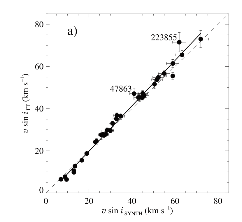
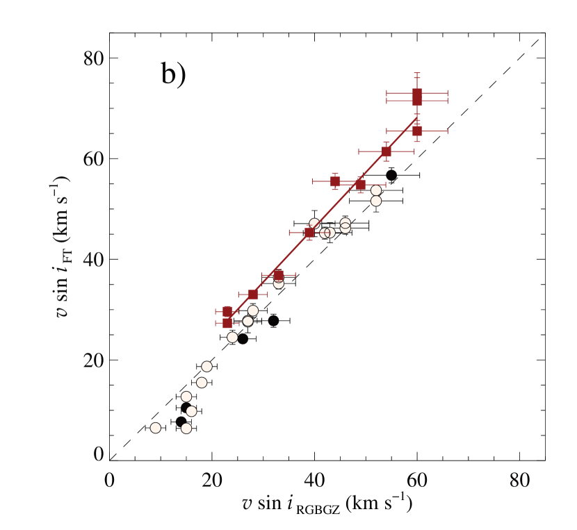
Figure 5: Comparison of the different $v\sin i$ determinations given in Table LABEL:tabstars, excluding SB2 stars. (a) The $v\sin i$ derived from the first zero of the FT is compared to the one derived from the spectral synthesis (SYNTH). The linear fit is shown by the thick solid line. The two stars with the largest differences are labeled. (b) The $v\sin i$ derived from the first zero of the FT is compared to the homogenized merged catalog from Royer et al. (2002b, RGBGZ). The different symbols stand from the source of the data in the latter: filled squares were from Abt & Morrell (1995, AM), filled circles were derived by RGBGZ using Fourier analysis, open circles are a combination of both sources. The linear fit on the subsample with data from AM is represented by the thick solid line. In both panels, the one-to-one relation is represented by the dashed line.

Figure 5b compares the new determinations to the homogenized values given by Royer et al. (2002b, RGBGZ). These latter determinations result from the merging of data from Abt & Morrell (1995, AM) and values derived from FT. The different symbols in the plot correspond to the combined source: AM only, FT only, or combination of both. The systematic overestimation at low $v\sin i$ in the determination from Royer et al. (2002b) results from the lower spectral resolution of ÉLODIE compared to SOPHIE in this work. A significant shift is noticed with the scaled values from AM, whereas no systematic effect is observed when comparing to values derived from FT. The linear relation between both scales (displayed in Fig. 5b) is given by:

$$v\sin i_{\mathrm{FT}}=(1.09\pm 0.03)\,v\sin i_{\mathrm{RGBGZ}}+2.8\pm 1.2.$$ (3)

The scaling relation between AM and the FT results is derived by Royer et al. (2002b) using spectral types from B8 to F2. This relation could slightly vary with the spectral type, as the comparison restricted to A0–A1-type stars suggests. The statistical correction applied by Royer et al. (2002b) is $v\sin i=1.05\,v\sin i_{\mathrm{AM}}+7.5$ and the resulting values for A0–A1 stars may be undercorrected.

6 Abundance analysis

For the rotational velocity range in our sample ($v\sin i\leq 65$ $\mbox{km}\,\mbox{s}^{-1}$), the most appropriate method to derive individual chemical abundances is the use of spectrum synthesis technique. Specifically, we iteratively adjust LTE synthetic spectra to the observed ones by minimizing the $\chi^{2}$ of the models to the observations using Takeda’s (1995) iterative procedure (see Gebran et al., 2008, for a detailed discussion).

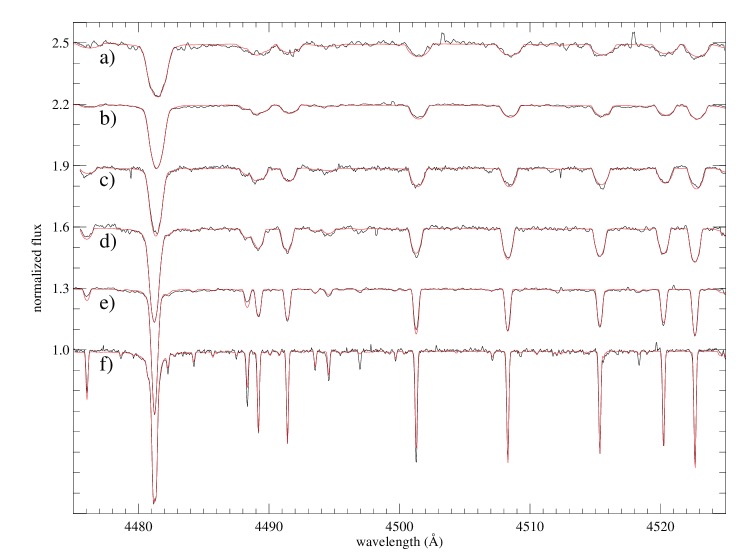
Figure 6: Selected observed spectra for six A-type stars with different values of $v\sin i$ (in black) shifted in flux by steps of 0.3 for clarity reasons. In red lines are the respective synthetic spectra in a region rich in Fe ii, Ti ii, and Mg ii lines. The spectra are sorted from top to bottom by decreasing $v\sin i$. The stars are (a) HD~101369, (b) HD~133962, (c) HD~107655, (d) HD~65900, (e) HD~58142 and (f) HD~72660. Spectra are shifted to rest wavelengths.

6.1 Spectrum synthesis

Table 4: Abundances for the 34 main-sequence targets not identified as contaminated. Ellipsis dots (…) stand for abundances that could not be determined for the corresponding object.

HD	[C/H]	[O/H]	[Mg/H]	[Si/H]	[Ca/H]	[Sc/H]	[Ti/H]	[Cr/H]	[Fe/H]	[Ni/H]	[Sr/H]	[Y/H]	[Zr/H]	[Ba/H]
1439	…	$0.018\pm 0.018$	$0.220\pm 0.140$	$0.231\pm 0.061$	$-0.232\pm 0.118$	$-0.098\pm 0.125$	$-0.023\pm 0.048$	$0.265\pm 0.135$	$0.072\pm 0.050$	…	$0.630\pm 0.150$	$0.685\pm 0.215$	$0.575\pm 0.004$	…
21050	$-0.360\pm 0.080$	$0.023\pm 0.041$	$0.170\pm 0.190$	$0.175\pm 0.010$	$-0.133\pm 0.138$	$-0.130\pm 0.237$	$-0.166\pm 0.056$	$0.278\pm 0.160$	$-0.075\pm 0.190$	…	$-0.350\pm 0.150$	…	$0.200\pm 0.185$	…
25175	$-0.365\pm 0.105$	$-0.010\pm 0.030$	$0.025\pm 0.145$	$0.180\pm 0.103$	$-0.115\pm 0.035$	$0.119\pm 0.104$	$-0.151\pm 0.092$	$0.118\pm 0.058$	$-0.160\pm 0.181$	$0.021\pm 0.311$	$-0.050\pm 0.150$	$0.046\pm 0.150$	$0.733\pm 0.077$	$0.817\pm 0.150$
28780	$-0.528\pm 0.047$	$-0.235\pm 0.065$	$-0.070\pm 0.190$	$-0.105\pm 0.175$	$-0.007\pm 0.234$	$-0.083\pm 0.068$	$0.013\pm 0.058$	$0.063\pm 0.098$	$-0.050\pm 0.088$	$0.280\pm 0.143$	$0.310\pm 0.150$	$0.225\pm 0.045$	$0.670\pm 0.116$	$0.744\pm 0.069$
30085	$-0.518\pm 0.061$	$-0.165\pm 0.015$	$-0.295\pm 0.092$	$0.056\pm 0.033$	$0.003\pm 0.053$	$-0.193\pm 0.179$	$0.163\pm 0.171$	$0.816\pm 0.357$	$-0.067\pm 0.155$	…	$1.118\pm 0.150$	$2.096\pm 0.024$	$2.062\pm 0.082$	$1.175\pm 0.035$
47863	$-0.185\pm 0.025$	$0.112\pm 0.150$	$0.153\pm 0.127$	$0.200\pm 0.000$	$0.310\pm 0.021$	$-0.057\pm 0.187$	$-0.432\pm 0.209$	$-0.014\pm 0.099$	$-0.270\pm 0.519$	$-0.039\pm 0.041$	$-0.758\pm 0.150$	$-0.128\pm 0.150$	$0.466\pm 0.024$	$0.830\pm 0.150$
58142	$-0.452\pm 0.056$	$-0.246\pm 0.056$	$-0.065\pm 0.175$	$0.269\pm 0.221$	$-0.057\pm 0.417$	$-0.466\pm 0.118$	$-0.165\pm 0.085$	$0.055\pm 0.078$	$-0.004\pm 0.124$	$0.287\pm 0.136$	$0.410\pm 0.150$	$0.313\pm 0.105$	$0.550\pm 0.097$	$0.912\pm 0.168$
65900	$-0.564\pm 0.379$	$-0.425\pm 0.058$	$0.073\pm 0.103$	$0.421\pm 0.223$	$0.063\pm 0.243$	$-0.298\pm 0.216$	$-0.029\pm 0.093$	$0.378\pm 0.076$	$0.247\pm 0.121$	$0.674\pm 0.093$	$0.805\pm 0.160$	$0.837\pm 0.097$	$1.123\pm 0.166$	$1.433\pm 0.150$
67959	$-0.403\pm 0.026$	$-0.270\pm 0.047$	$0.025\pm 0.245$	…	$-0.079\pm 0.015$	$-0.225\pm 0.167$	$0.153\pm 0.088$	$0.238\pm 0.068$	$0.190\pm 0.075$	$0.494\pm 0.115$	$0.786\pm 0.150$	…	…	…
72660	$-0.610\pm 0.082$	$-0.506\pm 0.066$	$0.094\pm 0.127$	$0.295\pm 0.025$	$0.053\pm 0.110$	$-0.245\pm 0.344$	$0.459\pm 0.114$	$0.800\pm 0.306$	$0.456\pm 0.061$	$0.696\pm 0.105$	$1.220\pm 0.150$	$0.835\pm 0.092$	$1.018\pm 0.051$	…
73316	$-0.308\pm 0.056$	$0.054\pm 0.050$	$0.056\pm 0.146$	$0.068\pm 0.034$	$0.036\pm 0.200$	$-0.374\pm 0.352$	$-0.072\pm 0.109$	$0.085\pm 0.082$	$-0.210\pm 0.132$	…	$-0.434\pm 0.150$	…	$0.430\pm 0.150$	$-0.096\pm 0.082$
83373	…	$-0.235\pm 0.005$	$0.095\pm 0.165$	$0.407\pm 0.055$	$-0.065\pm 0.025$	$0.073\pm 0.232$	$-0.166\pm 0.067$	$0.464\pm 0.168$	$0.099\pm 0.170$	…	$0.341\pm 0.150$	$0.886\pm 0.150$	$0.640\pm 0.120$	$1.110\pm 0.150$
85504	$0.251\pm 0.146$	$0.240\pm 0.076$	$0.412\pm 0.252$	$0.867\pm 0.351$	$0.129\pm 0.119$	$0.358\pm 0.234$	$-0.037\pm 0.088$	$0.382\pm 0.167$	$0.033\pm 0.111$	$0.260\pm 0.270$	$-0.238\pm 0.150$	$0.532\pm 0.172$	$0.613\pm 0.448$	…
89774	$-0.363\pm 0.027$	$0.167\pm 0.096$	$0.030\pm 0.204$	$0.149\pm 0.111$	$-0.097\pm 0.187$	$-0.269\pm 0.228$	$-0.115\pm 0.069$	$0.165\pm 0.073$	$-0.038\pm 0.149$	$0.057\pm 0.094$	$-0.099\pm 0.150$	$0.474\pm 0.013$	$0.919\pm 0.019$	$1.255\pm 0.385$
95418	$-0.510\pm 0.010$	$-0.327\pm 0.024$	$0.052\pm 0.128$	$0.438\pm 0.273$	$0.203\pm 0.195$	$-0.115\pm 0.107$	$-0.017\pm 0.041$	$0.318\pm 0.095$	$0.249\pm 0.110$	$0.400\pm 0.081$	$0.839\pm 0.156$	$0.750\pm 0.115$	$1.057\pm 0.143$	…
104181	$-0.040\pm 0.150$	$0.028\pm 0.007$	$0.090\pm 0.150$	$0.346\pm 0.317$	$-0.020\pm 0.150$	$0.200\pm 0.150$	$0.035\pm 0.175$	$-0.008\pm 0.102$	$-0.207\pm 0.025$	$-0.062\pm 0.399$	$-0.336\pm 0.150$	…	$0.750\pm 0.261$	…
107655	$-0.750\pm 0.150$	$-0.582\pm 0.150$	$-0.117\pm 0.150$	$0.039\pm 0.073$	…	$0.178\pm 0.066$	$-0.035\pm 0.116$	$0.559\pm 0.089$	$0.076\pm 0.055$	$0.771\pm 0.230$	$0.197\pm 0.150$	$0.798\pm 0.149$	$0.815\pm 0.176$	$0.715\pm 0.150$
127304	$-0.667\pm 0.029$	$-0.414\pm 0.050$	$0.013\pm 0.147$	$0.605\pm 0.316$	$-0.237\pm 0.161$	$-0.014\pm 0.150$	$0.070\pm 0.027$	$0.547\pm 0.174$	$0.233\pm 0.061$	$0.655\pm 0.166$	$0.780\pm 0.150$	…	$0.807\pm 0.081$	…
132145	$-0.180\pm 0.088$	$-0.145\pm 0.083$	$0.107\pm 0.183$	$0.271\pm 0.221$	$-0.068\pm 0.041$	$-0.130\pm 0.164$	$-0.076\pm 0.048$	$0.123\pm 0.049$	$-0.097\pm 0.126$	$-0.045\pm 0.174$	$-0.490\pm 0.150$	…	$0.254\pm 0.224$	…
133962	$-0.165\pm 0.033$	$-0.011\pm 0.020$	$0.005\pm 0.205$	$-0.115\pm 0.150$	$0.043\pm 0.037$	$0.000\pm 0.220$	$0.009\pm 0.079$	$0.112\pm 0.069$	$0.019\pm 0.185$	$0.422\pm 0.127$	$0.230\pm 0.150$	…	$0.520\pm 0.270$	…
145788	$-0.312\pm 0.165$	$0.048\pm 0.080$	$0.230\pm 0.140$	$0.265\pm 0.055$	$-0.165\pm 0.059$	$-0.310\pm 0.070$	$-0.145\pm 0.015$	$0.142\pm 0.082$	$-0.137\pm 0.149$	$0.120\pm 0.213$	$-0.430\pm 0.150$	$0.034\pm 0.085$	$0.180\pm 0.150$	…
154228	$-0.333\pm 0.385$	$-0.240\pm 0.150$	$0.060\pm 0.172$	$0.280\pm 0.030$	$-0.037\pm 0.504$	$-0.387\pm 0.128$	$-0.006\pm 0.060$	$0.433\pm 0.134$	$0.191\pm 0.074$	$0.440\pm 0.177$	$0.460\pm 0.150$	…	$0.763\pm 0.214$	…
156653	$-0.850\pm 0.110$	$-0.292\pm 0.030$	$-0.050\pm 0.280$	$0.008\pm 0.230$	$-0.175\pm 0.558$	$0.082\pm 0.072$	$-0.190\pm 0.057$	$0.133\pm 0.121$	$0.006\pm 0.102$	$0.037\pm 0.203$	$0.245\pm 0.150$	…	…	$0.803\pm 0.163$
158716	$-0.437\pm 0.136$	$-0.427\pm 0.101$	$0.055\pm 0.115$	$0.311\pm 0.007$	$-0.251\pm 0.387$	$-1.114\pm 0.150$	$0.192\pm 0.025$	$0.198\pm 0.013$	$0.235\pm 0.060$	$0.350\pm 0.113$	$0.490\pm 0.150$	$0.775\pm 0.035$	$0.755\pm 0.125$	…
172167	$-0.210\pm 0.154$	$-0.056\pm 0.115$	$-0.266\pm 0.176$	$-0.313\pm 0.184$	$-0.315\pm 0.548$	$-0.291\pm 0.199$	$-0.225\pm 0.297$	$-0.345\pm 0.144$	$-0.410\pm 0.096$	$0.047\pm 0.216$	$-0.845\pm 0.150$	…	$0.160\pm 0.170$	…
174567	$-0.450\pm 0.150$	$-0.085\pm 0.131$	$0.170\pm 0.250$	$0.195\pm 0.045$	$0.026\pm 0.217$	$-0.210\pm 0.150$	$-0.205\pm 0.055$	$0.190\pm 0.190$	$-0.036\pm 0.085$	$0.130\pm 0.150$	$-0.212\pm 0.150$	$0.218\pm 0.162$	$0.525\pm 0.065$	…
176984	$-0.133\pm 0.210$	$-0.205\pm 0.095$	$0.260\pm 0.230$	$0.140\pm 0.150$	$0.199\pm 0.226$	$-0.110\pm 0.150$	$-0.117\pm 0.043$	$0.263\pm 0.118$	$-0.276\pm 0.090$	$0.140\pm 0.450$	$0.240\pm 0.150$	$0.145\pm 0.205$	$0.043\pm 0.065$	…
196724	…	$-0.328\pm 0.087$	$0.080\pm 0.150$	$-0.030\pm 0.100$	$-0.186\pm 0.017$	$-0.214\pm 0.150$	$-0.314\pm 0.100$	$0.340\pm 0.224$	$0.008\pm 0.077$	$0.138\pm 0.150$	$0.198\pm 0.150$	$0.418\pm 0.174$	$0.585\pm 0.167$	…
198552	$-0.198\pm 0.082$	$-0.372\pm 0.032$	$-0.120\pm 0.139$	$0.095\pm 0.277$	$0.578\pm 0.392$	$-0.470\pm 0.214$	$-0.280\pm 0.035$	$0.039\pm 0.118$	$-0.069\pm 0.110$	$0.425\pm 0.122$	$-0.120\pm 0.150$	$0.150\pm 0.083$	$0.426\pm 0.092$	…
199095	$-0.177\pm 0.108$	$0.010\pm 0.073$	$-0.070\pm 0.314$	$0.105\pm 0.162$	$-0.043\pm 0.107$	$-0.185\pm 0.176$	$0.193\pm 0.160$	$0.089\pm 0.116$	$0.029\pm 0.078$	$0.330\pm 0.344$	$-0.040\pm 0.150$	…	$0.500\pm 0.040$	…
219290	$0.160\pm 0.150$	$-0.080\pm 0.057$	$0.100\pm 0.130$	$0.106\pm 0.032$	$-0.160\pm 0.151$	$-0.017\pm 0.048$	$-0.025\pm 0.070$	$0.278\pm 0.104$	$0.015\pm 0.038$	$0.640\pm 0.150$	$0.540\pm 0.150$	…	$0.503\pm 0.150$	…
219485	$-0.220\pm 0.150$	$-0.130\pm 0.021$	$0.140\pm 0.150$	$0.242\pm 0.352$	$-0.183\pm 0.050$	$-0.393\pm 0.111$	$-0.035\pm 0.045$	$0.232\pm 0.242$	$0.034\pm 0.099$	…	$0.550\pm 0.150$	$0.260\pm 0.113$	$0.500\pm 0.150$	…
223386	…	$-0.174\pm 0.081$	$0.126\pm 0.150$	$0.052\pm 0.126$	…	$-0.623\pm 0.257$	$-0.315\pm 0.065$	$0.130\pm 0.099$	$-0.227\pm 0.061$	…	$-0.300\pm 0.150$	$0.049\pm 0.051$	$-0.020\pm 0.150$	…
223855	$-0.163\pm 0.097$	$0.013\pm 0.090$	$0.270\pm 0.150$	$0.323\pm 0.386$	…	$-0.115\pm 0.085$	$-0.213\pm 0.042$	$0.022\pm 0.079$	$-0.036\pm 0.224$	…	$-0.730\pm 0.150$	$0.145\pm 0.105$	$0.340\pm 0.150$	…

Takeda’s procedure is divided in two parts. The first part is a modified version of Kurucz (1992) Width9 code and computes the opacity data. The second part of the routine computes the synthetic spectrum and minimizes the dispersion between the normalized synthetic spectrum and the observed one.

The line list used for spectral synthesis is the one used in Gebran et al. (2008, 2010). All transitions between 3000 and 7000 Å from Kurucz’s gfall.dat line list are selected for the calculation of the synthetic spectra. The abundance determination relies mainly on unblended transitions for about 14 chemical elements (C, O, Mg, Si, Ca, Sc, Ti, Cr, Fe, Ni, Sr, Y, Zr, and Ba). Most of these lines are weak because they are formed deep in the atmosphere. They are well suited to abundance determinations as LTE should prevail in the deeper layers of the atmospheres.

The accuracy of the atomic parameters (wavelengths, lower excitation potential, oscillator strength and damping constants) is checked against more accurate and/or more recent laboratory determinations, using the VALD (Kupka et al., 1999) and the NIST databases. The adopted atomic data for each elements are collected in Table 9, where for each element, the wavelength, the oscillator strength, and the reference are given.

A byproduct of this procedure is the derivation of the rotational ($v\sin i$) and the microturbulent ($\xi_{\mathrm{t}}$) velocities. We first derive the rotational and microturbulent velocities using several weak and moderately strong unblended Fe ii lines located between 4491.405 Å and 4522.634 Å and the Mg ii triplet around 4481 Å by allowing small variations around solar abundances of Mg and Fe as explained in Sect. 3.2.1 of Gebran et al. (2008). The weak iron lines are very sensitive to rotational velocity but not to microturbulent velocity while the moderately strong Fe ii lines are affected mostly by changes of microturbulent velocity. The Mg ii triplet is sensitive to both $\xi_{\mathrm{t}}$ and $v\sin i$. The derived rotational and microturbulent velocities are displayed in Table LABEL:tabstars. The error on $\xi_{\mathrm{t}}$ is $\pm 0.5$ $\mbox{km}\,\mbox{s}^{-1}$ (Gebran et al., 2010). By testing the effect of the variation of the $v\sin i$  on the abundance derived from the Mg ii triplet, we are able to determine $\Delta(v\sin i)$ that causes a variation of the abundance of about the error level ($\Delta[\mathrm{Mg/H}]\sim\sigma_{\mathrm{Mg}}$). On average we find that the rotational velocities have a precision estimated as 5% of the nominal $v\sin i$ and are in good agreement with those derived using the Fourier transforms (Sect. 5).

Once the rotational and microturbulent velocities are fixed, we then derive the abundance that minimized the $\chi^{2}$ for each transition of a given chemical element. Figure 6 displays the observed spectra of six A stars, for different $v\sin i$, with their respective best fit synthetic spectra.

6.2 Resulting abundances

The derived abundances are mean values and given in solar scale in Table 4, available online. For a given chemical element X, the abundance $\left[\mathrm{X/H}\right]$ is equal to the difference between the absolute abundance in the star $\log\left(\mathrm{X/H}\right)_{\star}$ and the abundance in the Sun $\log\left(\mathrm{X/H}\right)_{\odot}$ derived from Grevesse & Sauval (1998). As done in Gebran et al. (2008), errors on the elemental abundances are estimated by the standard deviation, assuming a Gaussian distribution of the abundances derived from each line. When only one line is measured, we adopted an average error on abundances derived from the results of Gebran et al. (2008, 2010) and Gebran & Monier (2008) for stars with $v\sin i$ $<$ 70 $\mbox{km}\,\mbox{s}^{-1}$. This error is found to be $\approx$ 0.15 dex.

7 Cluster analysis and classification

A quick look on the abundances listed in Table 4 and how these data are distributed in the Sr–Sc plane (Fig. 7b) suggests that several stars present CP characteristics. The size of our sample allows the use of statistical tools to disentangle the CP and normal stars and perform this classification in an automatic way, from the full abundance data set.

7.1 Classification criteria

In our temperature domain, the expected CP stars are the metallic Am stars (CP1) and the magnetic Ap stars (CP2). The classical definition of CP1 stars relies on Ca, Sc, iron-peak elements and heavy elements (Conti, 1970; Preston, 1974), and for the CP2 stars it is based on Si, Cr, Sr and Eu (Preston, 1974). Among the 14 species studied in this work, 10 species correspond to these classical definitions, i.e Si, Ca, Sc, Cr, Fe, Ni, Sr, Y, Zr and Ba.

7.2 Hierarchical cluster analysis

Hierarchical cluster analysis, applied to chemical abundances by Cowley & Bord (2004), is a bottom-up classification which consists in grouping data by proximity in a given space, producing a classification tree from single elements to the entire sample. It identifies clusters as a function of distance between elements. This method is applied to our data and clusters are searched for in the multi-dimensional space defined by the abundances from Table 4. Abundances are normalized so that the variation of a given elemental abundance over the full sample lies in the interval [$0,1$], ensuring that the different elements are equally weighted. Proximity is based on the Euclidean distance in the multi-dimensional normalized space. In the resulting classification tree (Fig. 7a), two main groups appear. They are identified as CP and normal stars, based on the median [Sr/H] abundance: this element being very discriminant (Fig. 7b), the group showing the highest median [Sr/H] abundance is associated with CP stars, and the other one with normal stars.

The construction of the classification tree does not take errors into account. In order to test the effect of the errors on the resulting memberships, new abundances are randomly simulated by adding Gaussian noise to the measured abundances, using the related standard deviation. Over 5000 simulations, targets are allocated to one group or the other, and the proportion of allocation to one group is taken as the final membership probability. This defines a new classification, taking the abundance errors into account.

This multivariate statistical analysis is performed using R (R Development Core Team, 2011).

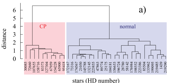
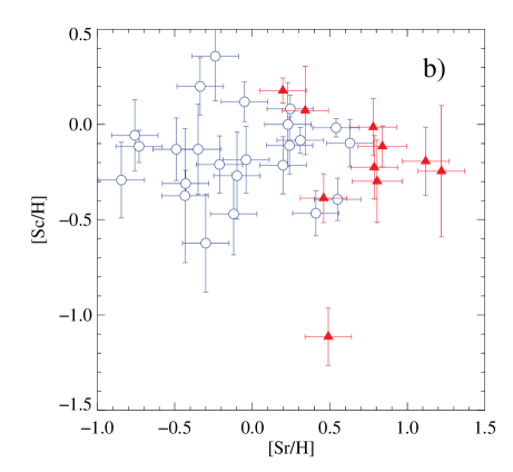
Figure 7: (a) Dendogram plot of the hierarchical tree resulting from the cluster analysis of the 14-species chemical abundances of the sample without errors. The x-axis gives the HD numbers of the stars and the y-axis represents the Euclidean distance, in the normalized abundance space, between subgroups. The two main groups are identified by the labeled boxes. (b) Scandium abundances as a function of strontium. The two main groups identified above are projected with different symbol: filled triangle stand for CP stars, open circles represent normal stars.

7.3 Resulting classification and comparison with literature data

Hierarchical cluster analysis is applied to the 14 species and produces the membership flag $f_{14}$ (1 for CP, 0 for normal) from the direct classification, for each star. The simulations taking errors into account give the membership probability $p_{14}$. Respectively, $f_{10}$ and $p_{10}$ are produced when applying hierarchical cluster analysis to the 10 “classical” species. Figure 8 displays these four criteria, also listed in Table 5 (available online).

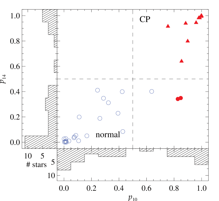
Figure 8: Membership to the CP group from the four criteria: probabilities using 10 and 14 species (respectively $p_{10}$ and $p_{14}$), direct classifications using 10 species (filled symbol for CP stars, open symbol for normal stars), and using 14 species (triangle for CP stars, circle for normal stars). Lower and left panels are the projected distributions of $p_{10}$ and $p_{14}$ respectively.

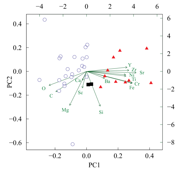
Figure 9: Observed sample and species projected on the first and second principal components (see text). The CP and normal stars are indicated by filled triangles and open circles respectively, according to the results from the cluster analysis. Filled squares represent the two uncertain objects and the open square stands for the probable normal star. The directions of the arrows show the relative loadings of the species on the first and second principal components.

The four criteria give rather consistent results. The distribution of $p_{14}$ shows slightly more separated and peaked groups than $p_{10}$, as a result of the additional discriminant species. A few objects show discrepant classifications: HD 219485 is classified as probably normal in Table 5 because the classification based on $p_{10}$ points it as a CP star whereas the other criteria indicate it is normal; two objects are classified as uncertain (HD 1439 and HD 219290) because the classification based on 10 species and the one based on 14 species produce contradictory results.

Table 5: Probabilities to be CP given by the four different criteria. Classification is deduced from the combination of four probabilities.

HD	$p_{10}$	$f_{10}$	$p_{14}$	$f_{14}$	Classification
1439	0.827	1	0.342	0	uncertain
21050	0.107	0	0.012	0	normal
25175	0.073	0	0.035	0	normal
28780	0.287	0	0.348	0	normal
30085	0.986	1	0.983	1	CP
47863	0.004	0	0.001	0	normal
58142	0.423	0	0.400	0	normal
65900	0.999	1	0.994	1	CP
67959	0.960	1	0.945	1	CP
72660	0.999	1	1.000	1	CP
73316	0.014	0	0.010	0	normal
83373	0.854	1	0.640	1	CP
85504	0.428	0	0.085	0	normal
89774	0.166	0	0.051	0	normal
95418	0.980	1	0.983	1	CP
104181	0.036	0	0.010	0	normal
107655	0.884	1	0.940	1	CP
127304	0.997	1	0.999	1	CP
132145	0.008	0	0.005	0	normal
133962	0.393	0	0.229	0	normal
145788	0.012	0	0.001	0	normal
154228	0.899	1	0.799	1	CP
156653	0.244	0	0.411	0	normal
158716	0.756	1	0.916	1	CP
172167	0.001	0	0.027	0	normal
174567	0.076	0	0.042	0	normal
176984	0.087	0	0.054	0	normal
196724	0.323	0	0.312	0	normal
198552	0.111	0	0.199	0	normal
199095	0.261	0	0.189	0	normal
219290	0.849	1	0.349	0	uncertain
219485	0.637	0	0.402	0	probably normal
223386	0.014	0	0.028	0	normal
223855	0.018	0	0.001	0	normal

In order to check how separated are the two groups in the chemical abundance space, we perform a principal component analysis to display the data in fewer dimensions. Principal component analysis is a statistical method that expresses a set of variables, possibly correlated, as a set of linearly uncorrelated variables called principal components. The principal components are linear combinations of the original variables and are defined in such a way that they have the largest possible variance. We apply this method to our data and derive the first two principal components from the 14-species abundances. The determined elemental abundances are projected onto these two new axes in Fig. 9, as well as the 14 axes corresponding to the different species. The first principal component (PC1) derived from the data explains 38.8% of the total variation and the second one (PC2) explains 15.4% of the variance in the 14-species abundances. Figure 9 shows that species from titanium to zirconium have strong positive loadings on PC1, whereas oxygen and carbon have strong negative loadings. On the other hand, PC2 has strong loadings from magnesium and silicium. The original data for the 34 stars are expressed in the first two components and overplotted in Fig. 9. They are represented according to the classification resulting from the cluster analysis. The dichotomy is very clear along the first principal component, and the objects identified as “uncertain” in Table 5 lie between the two groups.

Back in 2007, RZG used the release of the General Catalog of Ap and Am stars from Renson et al. (1991) to identify the chemically peculiar stars. This release is now outdated by Renson & Manfroid (2009). The 47 targets of our sample are not present in the previous version of the catalog, and the classification results can be compared with the content of the new release. Among these objects, nine are present in the catalog from Renson & Manfroid (2009), and are listed in Table 10. For two thirds of the common stars, both classifications are in agreement.

Table 6: Comparison of the classification with the General Catalog of Ap and Am stars (Renson & Manfroid, 2009).

HD	Renson & Manfroid (2009)		This work
58142		A0-A2	normal
72660		A1-	CP
83373	?	A1 Si	CP
85504		A1 Mn	normal
95418		A0- Ba Y	CP
107655	?	A1-	CP
127304	?	B9 Si	CP
145788	?	A1 Si	normal
154228	?	A1 Si	CP

On the other hand, four stars are classified as peculiar but are absent from the catalog built by Renson & Manfroid (2009): HD 30085, HD 65900, HD 67959, HD 158716. More details can be found in Appendix A.

8 Discussion

8.1 Abundance patterns

Figure 10 displays the median abundance patterns for the normal and peculiar stars resulting from our classification. Only fully agreeing classifications (all four criteria) are used to derive the median abundances, i.e. 21 normal stars and 10 CP stars. The dispersions are represented by the 16th and 84th percentiles, which in the Gaussian case correspond to the $\pm 1$-$\sigma$ standard deviation.

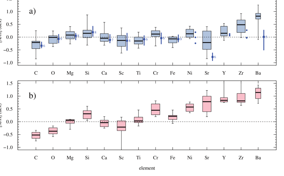
Figure 10: Abundance patterns are displayed as box and whisker plots for (a) the normal stars and (b) the CP stars. Boxes correspond to the 16th and 84th percentiles of the abundance distribution for each element, thick horizontal lines represent the median value, and the whiskers span from the minimum to the maximum values. The width of the boxes is proportional to the square root of the number of values. The horizontal dashed line stands for the solar values. In the top panel, median values and 16th and 84th percentiles derived from the comparison stars are plotted on the right side of the boxes, as filled squares and thick vertical lines. The number of abundance determinations is indicated when five or more abundances are available, and all individual determinations are displayed when the number is less than five (see Sect. 8.1).

The abundance pattern for the normal stars is compared with data from the Pleiades (Gebran & Monier, 2008) and from the Ursa Major moving group (Monier, 2005). We select nine normal A-type stars corresponding to our observed effective temperature range ($T_{\mathrm{eff}}>8900$ K): six stars are members of the Pleiades (HD 23763, HD 23948, HD 23629, HD 23632, HD 23489, HD 23387) and three belong to Ursa Major (HD 1404, HD 12471, HD 209515). They are analyzed by the latter authors using the same method and the code from Takeda (1995), ensuring a comparison with homogeneous data. Their median abundance pattern and the corresponding percentiles are overplotted in Fig. 10a. It should be noted that this comparison sample is small and does not fully cover all the species. The number of available determinations for each species in the comparison sample is indicated in the plot. The agreement between both patterns is very good but we notice discrepancies for strontium and the heavier elements. The comparison stars have on average a larger rotational broadening: seven of them have $100\leq v\sin i\leq 200$ $\mbox{km}\,\mbox{s}^{-1}$.

As far as the abundance pattern for the CP stars is concerned, no object shows a significant underabundance in calcium and the Ca abundance is very similar between CP and normal stars. This tendency is possibly due to the fact that previously known CP stars are not part of our sample. We find that carbon and oxygen are underabundant, in agreement with Roby & Lambert (1990). The iron-peak elements and heavy elements are overabundant, compared to the normal stars.

By construction, the $v\sin i$ range is limited in our sample. No clear trend of abundances versus $v\sin i$ is detected in our data, neither on the whole dataset nor considering both groups separately.

8.2 Rotational velocity distribution

Sections 3, 4 and 7 show that our sample is still contaminated by CP stars and binary stars. These new identifications allow the analysis of the rotational velocity distribution of normal stars with a much cleaner sample. It can be noticed that in our sample, no CP stars were found with $v\sin i\gtrsim 45$ $\mbox{km}\,\mbox{s}^{-1}$. The contamination by binary stars remains larger than by CP stars.

As defined in Sect. 2.4, our sample of 47 stars is the low $v\sin i$ part of a larger sample of 151 normal A0–A1 stars representing an 80%-complete, magnitude-limited volume. The distribution of rotational velocities of normal A0–A1 can be analyzed with this larger sample. The gray histogram in Fig. 11 represents the distribution of their observed $v\sin i$. By removing the 30 stars identified as peculiar and/or binaries in the previous sections, a cleaned subsample of 121 stars is selected, and its distribution of $v\sin i$ is showed by the hatched histogram (Fig. 11). The smoothed distributions of $v\sin i$ is obtained by applying the method described in Bowman & Azzalini (1997) and ported to R (R Development Core Team, 2011), and are shown by the dashed lines in Fig. 11. These distributions are then rectified from the projection effect to recover the distributions of equatorial velocities, assuming the rotation axes are randomly oriented (see RZG for details).

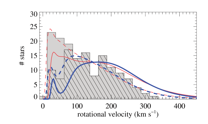
Figure 11: Distributions of rotational velocities: histograms are the observed $v\sin i$ (hatched histogram corresponds to the cleaned sample); dashed lines stand for the smoothed distribution of projected rotational velocities; solid lines are the distributions of equatorial velocities. Thick lines correspond to the newly cleaned sample of 121 stars whereas thin lines represent the full sample of 151 stars.

The high probability density for slow velocities disappears from the distribution in the cleaned sample, but a significant proportion (about 14%) of the normal stars rotates slowly at $v\leq 100$ $\mbox{km}\,\mbox{s}^{-1}$. These results considerably reduce the presence of slowly rotating normal A0–A1 stars. The overdensity at $v\leq 50\,\mbox{km}\,\mbox{s}^{-1}$ represents 4% of the distribution, i.e. five stars.

In the sample, the normal star with the lowest $v\sin i$ is HD 145788 ($v\sin i=9.8$ $\mbox{km}\,\mbox{s}^{-1}$ as measured from the ÉLODIE spectrum). In the rectified distribution, there is no star rotating more slowly than $v=20$ $\mbox{km}\,\mbox{s}^{-1}$.

9 Summary and conclusion

This work provides the spectroscopic study of a sample of 47 A0–A1 stars, initially selected from Royer et al. (2002b, 2007) to be main-sequence, low $v\sin i$, normal stars. The analysis of the cross-correlation profiles, and the variation of radial velocities allow the identification of suspected spectroscopic binaries. The spectral synthesis and the determination of chemical abundances are used to identify chemically peculiar stars using a hierarchical classification. The results reveal that two thirds of the sample is composed of spectroscopic binaries and chemically peculiar stars, and only 17 stars turn out to be normal, showing no sign of multiplicity nor peculiarity. The final composition of the sample is given by the pie chart in Fig. 12.

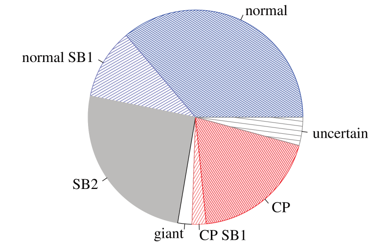
Figure 12: Resulting content of the sample of 47 A0–A1 stars.

In the framework of a nearly complete, magnitude limited sample of 121 A0–A1-type normal stars, this implies that the distribution of equatorial velocities, under the assumption of randomly oriented rotation axes, is no longer dominated by a large fraction of slowly rotating stars. Only 14% of the A0–A1 normal stars are rotating at $v\leq 100$ $\mbox{km}\,\mbox{s}^{-1}$, which correspond to about 16 objects, and 21% are rotating at $v\leq 120$ $\mbox{km}\,\mbox{s}^{-1}$. This is to be compared with the corresponding proportions in the non-cleaned sample: 31% and 37% respectively (Fig. 11). The distribution is not bimodal as previously claimed by RZG, but the overlap with the distribution of equatorial velocity of CP stars seems real, contrary to the conclusion of Abt & Morrell (1995) and Abt (2000).

Table 7: List of HD identifiers for the single normal stars. The ones written in boldface are suspected to be doubtful candidates from the comparison with literature data (see Appendix A).

21050	25175	28780	47863	58142	73316	85504
89774	104181	132145	133962	145788	172167	198552
219485	223386	223855

The 17 normal stars, spectroscopically identified in this paper, are listed in Table 7. The objects were not extensively monitored in terms of radial velocity and spectroscopic binarity may still remain undetected in this sample. Possibly doubtful candidates are indicated in Table 7, which could be either spectroscopic binaries or marginal CP stars (see Appendix A). The 17 normal stars will be more deeply investigated in a forthcoming paper to check whether signatures of gravity darkening due to fast rotation seen pole-on are present in the spectra. If rotation axes are randomly oriented, the probability to observe a star with $i\leq 10\degr$ is about 1.5%, which would produce just two stars among the 121 normal A0–A1 stars.

Appendix A Comments on individual stars

All our targets are part of the sample studied by Dworetsky (1974), and 25 of them are analyzed by Ramella et al. (1989). In their paper, Ramella et al. (1989) derive $v\sin i$ from Fourier profile analysis and flag the stars according to the agreement between the observed profile and a theoretical rotation profile (‘1’ when agreeing, ‘0’ when disagreeing, in their Table 3). Stars labeled as ‘0’ by Ramella et al. are checked out with our data, and the Fourier profiles are plotted in Fig. 15.

Gontcharov (2006) published a compilation of radial velocities and our individual measurements are compared with literature data. The 44 stars in common are plotted in Fig. 13. The Gaussian fit of the histogram of radial velocity differences gives a standard deviation $\sigma=2\,\mbox{km}\,\mbox{s}^{-1}$. Ten stars show differences larger than $3\,\sigma$. They are indicated in Fig. 13. The three stars of our sample (HD 40446, HD 119537 and HD 176984), that are not present in Gontcharov (2006), are already detected as binaries in our data.

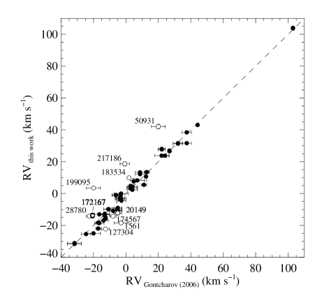
Figure 13: Comparison of radial velocities between individual values from Table LABEL:indivspectra and the compilation from Gontcharov (2006). The error bars are the internal errors and the dashed line is the one-to-one relation. The outliers are indicated by open symbols, together with their HD number.

HD~1439

could not be undoubtedly classified as a normal nor CP star, the derived memberships based on 10 and 14 elements giving contradictory results (Table 5). It moreover lies in the “uncertain” zone in Fig. 9. The derived abundances in oxygen and magnesium are high enough to make it classified as a normal star using all 14 elements whereas the remaining pattern (Si, Ca, Sc, Cr, Fe, Sr, Y and Zr) is rather similar to a CP star. Its radial velocity observed 18 months apart does not show significant variation.

HD~1561

is variable in radial velocity, from our two observations as well as compared with Gontcharov (2006) who gives a radial velocity of $-3\,\mbox{km}\,\mbox{s}^{-1}$ (Fig. 13).

HD~6530

is detected as a spectroscopic binary from its CCF (Fig. 2). The large difference in the $v\sin i$ measured using the spectral synthesis and the FT (Table LABEL:tabstars) is due to the composite spectrum. It has already been observed by Grenier et al. (1999) who derive the radial velocity and their spectrum is also used by Royer et al. (2002a) to derive the $v\sin i$. The CCF from this spectrum is overplotted in Fig.14 (black solid line) to emphasize the binary nature of the star.

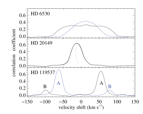
Figure 14: Cross-correlation functions for three suspected binary stars. Top panel: the CCF of the observed spectrum is overplotted to the one observed by Grenier et al. (1999). Middle panel: the bisector of the CCF is displayed (dotted line) with a velocity scale enhanced by a factor 3, for the sake of clarity. Bottom panel: The two components in the composite CCF are labeled as ‘A’ and ‘B’.

HD~20149

is flagged as a suspected binary due to the asymmetry of the CCF. The bisector is displayed in Fig.14. The star is labeled as variable in radial velocity in Gontcharov (2006), and the published value ($-5\,\mbox{km}\,\mbox{s}^{-1}$) is also significantly different from our determinations (Fig. 13).

HD~21050

is found to have a large projected rotational velocity by Dworetsky (1974) ($v\sin i=60\,\mbox{km}\,\mbox{s}^{-1}$) but all other determinations are very similar to our result (Palmer et al., 1968; Abt & Morrell, 1995; Royer et al., 2002b). Moreover, no spectral variation is detected in our high signal-to-noise observations, collected three years apart.

HD~25175

is suspected by Ramella et al. (1989) to be a spectroscopic binary due to the large broadening and the disagreement the observed profile and a theoretical rotational profile. Their determination of $v\sin i$, in good agreement with ours, is much higher than the value derived by Dworetsky (1974) ($\leq 40\,\mbox{km}\,\mbox{s}^{-1}$). Our Fourier profiles are plotted in Fig. 15a and the agreement with the rotational profile is very good, suggesting that the broadening is dominated by rotation. Also both our spectra, observed one year apart, do not show any sign of radial velocity variation.

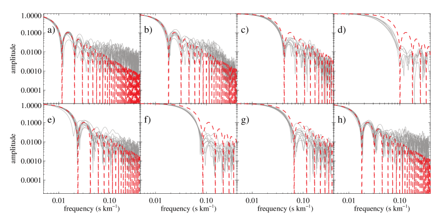
Figure 15: Individual line FT (solid lines) and theoretical rotation profile corresponding to the average $v\sin i$ (thick dashed line) for the stars flagged as ‘0’ by Ramella et al. (1989): (a) HD 25175, (b) HD 65900, (c) HD 67959, (d) HD 72660, (e) HD 85504, (f) HD 127304, (g) HD 145788, (h) HD 223386.

HD~28780

has a $v\sin i$ significantly different from what Ramella et al. (1989) find (41.3 $\mbox{km}\,\mbox{s}^{-1}$). The radial velocity is moreover significantly different from the value published by Gontcharov (2006): $-22.6\,\mbox{km}\,\mbox{s}^{-1}$ (Fig. 13). Although no evidence of binarity is detected in our single observation, these differences suggest that this object could be a spectroscopic binary.

HD~30085

is discarded from $v\sin i$ measurement by Ramella et al. (1989) because of asymmetric line profiles. In our classification, it falls in the CP group and is newly detected as chemically peculiar.

HD~33654

is identified as a giant star from both its surface gravity and its luminosity (Table LABEL:tabstars), which disagrees with its luminosity class: A0V. It was previously classified as a B9III star (Palmer et al., 1968). It is indicated as an Ap Si star in Renson & Manfroid (2009).

HD~39985

is an outlier in our luminosity comparison (Fig. 3) and therefore suspected to be a binary star.

HD~40446

is flagged as a spectroscopic binary by Dworetsky (1974). It is part of the sample studied by Royer et al. (2002b) who determined an uncertain $v\sin i$ with a high external error ($v\sin i=27\mbox{:}\pm 5\,\mbox{km}\,\mbox{s}^{-1}$) due to a large dispersion in the values derived from individual lines. Its binary nature is confirmed by the shape of its CCF in Fig. 2.

HD~46642

is suspected to be a photometric variable star (Kukarkin et al., 1981). Our radial velocity measurements reveal a variation hence this star is suspected to be a binary.

HD~47863

shows a significant difference between our measurements of $v\sin i$, using spectral synthesis and Fourier profile. This object is however used as a reference star in speckle observations by Aristidi et al. (1997), suggesting that it is a single star.

HD~50931

is detected as a spectroscopic binary from the distorted shape of its CCF. The radial velocity from Gontcharov (2006) is moreover very different from our result: 20 $\mbox{km}\,\mbox{s}^{-1}$ (Fig. 13). The large difference in the $v\sin i$ measured using the spectral synthesis and the FT (respectively 75 and 84 $\mbox{km}\,\mbox{s}^{-1}$ in Table LABEL:tabstars) is due to the composite spectrum.

HD~58142

is found to be a hot Am star by Adelman (1994), which disagrees with our classification. This object lies in the tail of the distribution of memberships (Table 5 and Fig. 8) and could have been wrongly assigned to the “normal” group.

HD~65900

is suspected by Ramella et al. (1989) to be a spectroscopic binary due to the large broadening and the disagreement between the observed profile and a theoretical rotational profile. This disagreement is not seen in our data (Fig. 15b). In our classification, it falls in the CP group and is newly detected as chemically peculiar.

HD~67959

is found to disagree with a rotation profile by Ramella et al. (1989), but this is very probably due to its low $v\sin i$ and the fact that instrumental broadening is not negligible. In our data (Fig. 15c), the main lobe of the FT in observed profiles is well fitted by the theoretical rotation profile. In our classification, it falls in the CP group and is newly detected as chemically peculiar.

HD~72660

is a hot Am star (Varenne, 1999), which is consistent with our classification. Its low $v\sin i$ makes the Fourier profiles dominated by the instrumental profile, both in Ramella et al. (1989) and in Fig. 15d. It is listed in Table 3 as variable in radial velocity, but the variation remains very small. Landstreet (1998) detects an asymmetry in the spectral lines that is attributed to a depth-dependent velocity field.

HD~85504

is flagged by Ramella et al. (1989) as showing a profile disagreeing with a rotational broadening. In our data however (Fig. 15e), the agreement with the theoretical rotational profile is good. This object is flagged in Renson & Manfroid (2009) as an Ap Mn star, and manganese is not part of our analyzed chemical species. In Adelman & Pintado (1997), it only appears slightly metal rich compared to other superficially normal stars with similar effective temperature. This object is moreover known as high spacial velocity (Martinet, 1970; Altmann & de Boer, 2000) which may be a runaway star. It is a suspected variable star (Kukarkin et al., 1981).

HD~95418

is an Am star (Adelman et al., 2011; Hill, 1995) and our classification agrees with these results.

HD~101369

is suspected to be a spectroscopic binary from the shape of its CCF (Fig. 2).

HD~107655

belongs to the open cluster Coma Ber. Gebran et al. (2008) derived abundances, using the same method, and their values are in good agreement with our determinations, with larger differences for Sc and Sr. The dispersion in the Sc and Sr abundances derived by Gebran et al. (2008) is high; they include more lines than in this study, especially lines located in the wings of Balmer lines. When restricting the comparison to lines in common, the agreement is much better (Table 8).

Table 8: Comparison of Sc and Sr abundances of HD~107655 with Gebran et al. (2008). The mean abundances, relative to the Sun, are given, as well as the absolute abundances for each spectral line. Ellipsis dots (…) indicate when a spectral line has not been used.

Element / line	this study	Gebran et al. (2008)
[Sc/H]	$0.178\pm 0.066$	$-0.2\pm 0.11$
4314.083 Å	…	2.55
4320.732 Å	…	3.02
4324.996 Å	…	2.81
4374.457 Å	3.374	3.14
5657.896 Å	3.243	3.13
[Sr/H]	$0.197\pm 0.150$	$-0.23\pm 0.20$
4077.709 Å	…	2.29
4215.520 Å	3.127	3.08

HD~119537

is detected as a spectroscopic binary by Dworetsky (1974). The SB2 nature is clearly visible in our CCFs and they are plotted for both observations in Fig.14 together with the labels of the components (‘A’ being the component with the highest correlation peak). The radial velocities given in Table LABEL:indivspectra are the one corresponding to component A and the difference in radial velocity (A$-$B) is $153.4\,\mbox{km}\,\mbox{s}^{-1}$ in the first observation (2006-06-02) and $-140.9\,\mbox{km}\,\mbox{s}^{-1}$ on the second (2012-02-14).

HD~127304

is suspected by Ramella et al. (1989) to be a SB2. Our derived radial velocity is moreover significantly different from the value published by Gontcharov (2006), $-12.6\,\mbox{km}\,\mbox{s}^{-1}$ (Fig. 13).

HD~132145

is suspected by Ramella et al. (1989) to be a spectroscopic binary. The observed variation in radial velocity in our data is not significant taking the instrumental offset between both spectrographs into account.

HD~133962

is suspected to be a photometric variable star (Kukarkin et al., 1981).

HD~145647

is suspected to be a binary star from the shape of the CCF (Fig. 2).

HD~145788

is studied by Fossati et al. (2009) who do not detect clear signatures of chemical peculiarity and believe this object is a normal star whose abundance pattern reflects the composition of its progenitor cloud. It is flagged by Ramella et al. (1989) as showing a profile disagreeing with a rotational broadening, probably due to the small rotational broadening. In Fig. 15g, the shape of the main lobes of the observed profiles agree with the theoretical rotation profile. This star was only observed with ÉLODIE and in our classification, it falls in the normal group. In the sample, it is the normal star with the smallest $v\sin i$.

HD~156653

is indicated as a spectroscopic binary by Dworetsky (1974). Our radial velocity measurements show a ratio of the external error over the internal error just above the threshold used to identify variations in Table 3.

HD~158716

is suspected by Ramella et al. (1989) to be a spectroscopic binary. In our classification, it falls in the CP group and is newly detected as chemically peculiar.

HD~172167

is, strangely enough, an outlier in Fig. 13, where Gontcharov (2006) gives a radial velocity of $-20.6\,\mbox{km}\,\mbox{s}^{-1}$. Vega is not known to have a variable radial velocity on such a scale.

HD~174567

is suspected by Ramella et al. (1989) to be a variable CP star (strong Si and variable Sr). It is classified as a normal star according to our measurements but we detect a variation in radial velocity, strengthened by the comparison with Gontcharov (2006) in Fig. 13.

HD~176984

is suspected to be a spectroscopic binary from the variability of its radial velocity (Table 3).

HD~183534

is detected as a spectroscopic binary from the shape of its CCF (Fig. 2) and the difference in radial velocity with Gontcharov (2006) in Fig. 13.

HD~196724

is suspected to be a spectroscopic binary from the variability of its radial velocity (Table 3).

HD~199095

is detected as a spectroscopic binary by Dworetsky (1974). Our measurements show a variation in radial velocity, confirmed when comparing with data from Gontcharov (2006) in Fig. 13.

HD~217186

is considered to be a possible magnetic field candidate by Schröder et al. (2008) after being associated with a ROSAT X-ray source (Schröder & Schmitt, 2007) as a bona fide single star. This object is however suspected to be a binary from the shape of its CCF (Fig. 2). We have only one spectrum for this object, but the comparison with Gontcharov (2006), in Fig. 13, suggests a variation in radial velocity.

HD~219290

is listed as “uncertain” in Table 5 and lies in the “uncertain” zone in Fig. 9. The high abundances in carbon and oxygen produce contradictory classifications when 10 and 14 are used. The remaining pattern (Si, Ca, Sc, Cr, Fe, Ni, Sr and Zr) is rather similar to a CP star.

HD~219485

is listed as “probably normal” in Table 5. It is marginally classified as a CP star based on the 10 “classical” elements. The abundances in Ni and Sr are however significantly higher than the median values in the normal star pattern displayed in Fig. 10.

HD~223386

is flagged as disagreeing from a rotation profile by Ramella et al. (1989), but the agreement is very good in our data (Fig. 15h).

HD~223855

is indicated as a spectroscopic binary by Dworetsky (1974). It shows a significant difference between the measurements of $v\sin i$ using spectral synthesis and Fourier profiles, and both values are significantly higher than the one derived by Dworetsky (1974): $45\,\mbox{km}\,\mbox{s}^{-1}$.

Appendix B Linelist

The analyzed spectral lines are listed in Table 9, sorted by chemical element and central wavelength, together with the adopted oscillator strength.

Table 9: Atomic data and their reference for the lines used in our abundances determination.

Element	$\lambda$ (Å)	$\log gf$	Ref.	Element	$\lambda$ (Å)	$\log gf$	Ref.	Element	$\lambda$ (Å)	$\log gf$	Ref.
C i	4932.049	$-1.658$	1	Sc ii	4246.822	$0.242$	1	Ni i	4470.472	$-0.310$	3
C i	5052.167	$-1.303$	1	Sc ii	4374.457	$-0.418$	1	Ni i	4480.561	$-1.491$	3
C i	5380.337	$-1.616$	1	Sc ii	4670.407	$-0.576$	1	Ni i	4490.049	$-2.108$	3
C i	5793.120	$-2.063$	1	Sc ii	5031.021	$-0.400$	1	Ni i	4490.525	$-2.324$	3
C i	5800.602	$-2.337$	1	Sc ii	5239.813	$-0.765$	1	Ni i	4604.982	$-0.250$	3
O i	5330.726	$-2.416$	1	Sc ii	5526.790	$0.020$	1	Ni i	4648.646	$-0.100$	3
O i	5330.735	$-1.570$	1	Sc ii	5657.896	$-0.603$	1	Ni i	5080.528	$0.330$	3
O i	5330.741	$-0.983$	1	Ti ii	4163.644	$-0.130$	4	Ni i	5099.927	$-0.100$	3
O i	6155.961	$-1.363$	1	Ti ii	4287.873	$-1.790$	4	Ni i	5476.904	$-0.890$	1
O i	6155.961	$-1.363$	1	Ti ii	4417.714	$-1.190$	4	Sr ii	4215.520	$-0.169$	1
O i	6155.971	$-1.011$	1	Ti ii	4443.801	$-0.720$	4	Y ii	4883.684	$0.070$	3
O i	6155.989	$-1.120$	1	Ti ii	4468.492	$-0.600$	5	Y ii	4900.120	$-0.090$	3
O i	6156.737	$-1.487$	1	Ti ii	4501.270	$-0.770$	4	Y ii	5087.416	$-0.170$	3
O i	6156.755	$-0.898$	1	Cr ii	4592.049	$-1.217$	5	Y ii	5200.406	$-0.570$	3
O i	6156.778	$-0.694$	1	Cr ii	4616.629	$-1.291$	6	Zr ii	4156.240	$-0.776$	3
O i	6158.149	$-1.841$	1	Cr ii	4634.070	$-0.990$	3	Zr ii	4161.210	$-0.720$	3
O i	6158.172	$-0.995$	1	Cr ii	4812.337	$-1.995$	3	Zr ii	4208.980	$-0.460$	3
O i	6158.187	$-0.409$	1	Cr ii	5237.329	$-1.160$	5	Zr ii	4496.960	$-0.810$	7
Mg ii	4427.994	$-1.201$	1	Cr ii	5308.440	$-1.810$	5	Ba ii	4554.029	$0.163$	3
Mg ii	4481.126	$0.730$	2	Cr ii	5313.590	$-1.650$	5	Ba ii	4934.076	$-0.156$	8
Mg ii	4481.150	$-0.570$	2	Fe ii	4273.326	$-3.258$	5	Ba ii	6141.713	$-0.810$	1
Mg ii	4481.325	$0.575$	2	Fe ii	4296.572	$-3.010$	5
Si ii	5041.024	$0.174$	1	Fe ii	4416.830	$-2.600$	5
Si ii	5055.984	$0.441$	1	Fe ii	4491.405	$-2.690$	5
Si ii	5056.317	$-0.535$	1	Fe ii	4508.288	$-2.210$	5
Si ii	5466.432	$-0.190$	3	Fe ii	4515.339	$-2.490$	5
Si ii	5688.817	$0.106$	1	Fe ii	4520.224	$-2.600$	5
Si ii	5978.930	$-0.061$	1	Fe ii	4522.634	$-2.030$	5
Ca ii	4489.179	$-0.726$	3	Fe ii	4541.524	$-3.050$	5
Ca ii	4489.179	$-2.157$	3	Fe ii	4555.890	$-2.290$	5
Ca ii	4489.179	$-0.613$	3	Fe ii	4582.835	$-3.100$	5
Ca ii	5001.479	$-0.517$	1	Fe ii	4656.981	$-3.630$	5
Ca ii	5019.971	$-0.257$	1	Fe ii	4666.758	$-3.330$	5
Ca ii	5021.138	$-1.217$	1	Fe ii	4923.927	$-1.320$	5
Ca ii	5285.266	$-1.153$	1	Fe ii	5197.577	$-2.100$	5
Ca ii	5307.224	$-0.853$	1	Fe ii	5276.002	$-1.940$	5
				Fe ii	5316.615	$-1.850$	5

(1) NIST; (2) Biermann & Lübeck (1948); (3) Kurucz (http://kurucz.harvard.edu/LINELISTS/GFALL); (4) Pickering et al. (2002); (5) Fuhr et al. (1988); (6) Sigut & Landstreet (1990); (7) Biemont et al. (1981); (8) Miles & Wiese (1969).