Large-$n$ conditional facedness $m_{n}$
of 3D Poisson-Voronoi cells

Abstract

We consider the three-dimensional Poisson-Voronoi tessellation and study the average facedness $m_{n}$ of a cell known to neighbor an $n$-faced cell. Whereas Aboav’s law states that $m_{n}=A+Bn^{-1}$, theoretical arguments indicate an asymptotic expansion $m_{n}=8+k_{1}n^{-1/6}+\ldots$. Recent new Monte Carlo data due to Lazar et al., based on a very large data set, now clearly rule out Aboav’s law. In this work we determine the numerical value of $k_{1}$ and compare the expansion to the Monte Carlo data. The calculation of $k_{1}$ involves an auxiliary planar cellular structure composed of circular arcs, that we will call the Poisson-Möbius diagram. It is a special case of more general Möbius diagrams (or multiplicatively weighted power diagrams) and is of interest for its own sake. We obtain exact results for the total edge length per unit area, which is a prerequisite for the coefficient $k_{1}$, and a few other quantities in this diagram.

Keywords: Poisson-Voronoi diagram, Aboav’s law, Möbius diagram, large-$n$ behavior

LPT-Orsay-14-01

1 Introduction

C ellular structures, or spatial tessellations, are of interest because of their very wide applicability. The perhaps simplest model of a cellular structure is the Poisson-Voronoi tessellation (or ‘diagram’), obtained by constructing the Voronoi cells around pointlike ‘seeds’ distributed randomly and uniformly in space. Whereas two- and three-dimensional Poisson-Voronoi diagrams are relevant for real-life cellular structures, the higher-dimensional case appears in data analyses of various kinds. An excellent overview of the many applications is given in the monograph by Okabe et al. [1].

Beginning with the early work of Meijering [2], much theoretical effort has been spent on finding exact analytic expressions for the basic statistical properties of the Voronoi tessellation, in particular in spatial dimensions $d=2$ and $d=3$, but also in higher dimensions.

Of interest is first of all is the probability $p_{n}(d)$ that a cell have exactly $n$ sides (in dimension $d=2$) or $n$ faces (in dimension $d=3$). Next comes the conditional sidedness (or facedness), usually denoted $m_{n}(d)$, i.e. the average number of sides (or faces) of a cell known to neighbor an $n$-sided (or $n$-faced) cell. There has been considerable theoretical interest in the dependence of $p_{n}(d)$ and $m_{n}(d)$ on $n$, but only very few analytic results exist. In this work we will be interested in $m_{n}(2)$ and $m_{n}(3)$.

In two dimensions experimental data are fairly numerous but usually cover a limited range of $n$ values, not beyond $n\approx 10$. The data are most often plotted as $nm_{n}$ versus  $n$. In the experimental range it has often been possible to fit them by what is known as Aboav’s ‘linear’ law [3], which says that $nm_{n}=An+B$, where $A$ and $B$ are adjustable parameters. On the basis of Monte Carlo simulations [4] it has been known since a long time, however, that two-dimensional Poisson-Voronoi cells violate Aboav’s law, the graph of $nm_{n}$ being slightly but definitely curved.

In earlier work [5, 6, 7] we have been interested in Voronoi cells with a very large number $n$ of sides (or faces). We determined the exact asymptotic behavior of $p_{n}(2)$ in the large $n$ limit and deduced [8] from it, under very plausible hypotheses, the asymptotic behavior of $m_{n}$,

$$m_{n}(2)=4+3(\pi/n)^{\frac{1}{2}}+\ldots,\qquad n\to\infty,$$ (1.1)

which rules out Aboav’s law. When truncated after the second term, Eq. (1.1) is in quite reasonable agreement with the Monte Carlo data. An extension [9] of these arguments to higher dimensions, under plausible but unproven assumptions, led to

$$m_{n}(3)=8+k_{1}n^{-\frac{1}{6}}+\ldots,\qquad n\to\infty.$$ (1.2)

Apart from the precise structure of this formula, its most important prediction is that Aboav’s linear law is violated also by three-dimensional Poisson-Voronoi cells. At the time, however, the existing $d=3$ Monte Carlo data were insufficiently precise to confirm this. Indeed, three-dimensional Monte Carlo results due to Kumar et al. [10] covering the range $10\leq n\leq 22$ were interpreted by Fortes [11] in terms of Aboav’s law.

The situation has changed recently due to an impressive large scale Monte Carlo simulation by Lazar et al. [12], which provides a rich trove of information about the three-dimensional Poisson-Voronoi tessellation. Amidst a wealth of other data the authors determine the values $m_{n}(3)$ based on a data set of 250 million Voronoi cells. Their results clearly show the nonlinearity of $nm_{n}(3)$. Given these new data it therefore becomes of interest to consider again the asymptotic expansion (1.2) and to try and determine the numerical value of the coefficient $k_{1}$. We do so in this paper and compare the result to the Monte Carlo data of Lazar et al. A juxtaposition of the two- and the three-dimensional $m_{n}$ is also illuminating.

In section 2 we recall how the question of calculating the three-dimensional $m_{n}$ in the large-$n$ limit leads to the problem of a special (non-Voronoi) tessellation on a spherical surface of radius $\sim n^{1/3}$, i.e. essentially a two-dimensional problem. This tessellation, whose edges are circular arcs, is of interest in its own right. It is closely related to the multiplicatively weighted (or: Möbius) diagrams reviewed in Ref. [1], which is why we call it the Poisson-Möbius  diagram.

Section 3 deals with this auxiliary problem and may be read independently of the rest of the paper. We derive the exact expression for a prerequisite for finding $k_{1}$, viz. the average edge length per unit area in the Poisson-Möbius diagram.

In section 4 we briefly describe some Monte Carlo work that we did on this tessellation.

In section 5 we the return to the three-dimensional $m_{n}(3)$ and provide extensions of Eq. (1.2).

2 The many-faced 3D Poisson-Voronoi cell

We consider a three-dimensional Poisson-Voronoi diagram of seed density $\rho$. This density may be scaled to unity but we will keep it as a check on dimensional consistency. Let the cell of a central seed have $n$ faces. It was argued in Ref. [9] that in the limit of large $n$ certain cell properties become deterministic, in analogy to what happens in a statistical system in the thermodynamic limit. In particular, in the limit of large $n$ the $n$ first-neighbor seeds $\mathbf{F}_{j}$ lie in a spherical shell of radius $R_{n}\simeq(3n/4\pi\rho)^{1/3}$ (this radius was called $2R_{*}$ in Ref. [9]) and of effective width $\sim n^{-2/3}$. For the present purpose this width may be set to zero and for $n\to\infty$ the shell may be approximated locally by a flat plane ${\cal F}$ as shown in Fig. 1.

Also in that limit, the Voronoi cells of the first neighbors $\mathbf{F}_{j}$ approach prisms that intersect ${\cal F}$ according to the two-dimensional Voronoi diagram of the set of seeds $\{\mathbf{F}_{j}\}$. There is no reason for these seeds to be Poisson distributed, but their average sidedness is necessarily exactly six, which is therefore also the average number of lateral faces of a prism. Each prism furthermore has at its lower end a face in common with the central Voronoi cell, not shown in the figure. At their upper ends the prisms have faces in common with the second-neighbor cells constructed around the seeds $\mathbf{S}_{1},\mathbf{S}_{2},\ldots$. A key observation is that for $n\to\infty$ the first-neighbor seeds become infinitely dense in ${\cal F}$, and that in that limit the surface (to be called $\Gamma$) separating the second-neighbor cells from the first-neighbor ones becomes piecewise paraboloidal, the piece ${\cal P}_{j}$ (see Fig. 1) lying on the paraboloid of revolution equidistant from $\mathbf{S}_{j}$ and from ${\cal F}$. The second-neighbor seeds have an $n$ independent spacing $\sim\rho^{-1/3}$ between themselves, whereas the typical diameter of a prism vanishes as $\sim n^{-1/6}$.

Fig. 1 shows to the left the generic case where a first-neighbor cell around a seed $\mathbf{F}_{0}$ has a single face at its upper end. This happens with a probability, to be called $f_{8}$, that tends to unity when $n\to\infty$. The same figure shows to the right the exceptional case where the upper end of a first-neighbor cell around a seed $\mathbf{F}_{1}$ has two faces in common with the second-neighbor cells. We denote the probability for this to happen by $f_{9}$. This event occurs only when the upper end of the prism intersects the joint between two paraboloidal surface segments. In the figure to the right, the arc $AB$ is such a joint, itself located in the plane ${\cal Q}$ that perpendicularly bisects the vector $\mathbf{S}_{1}-\mathbf{S}_{2}$. In Ref. [9] it was argued that $f_{8}=1-{\cal O}(n^{-1/6})$ and that $f_{9}=k_{1}n^{-1/6}+\ldots$, whereas the analogously defined probabilities $f_{10}$ and beyond are proportional to higher powers of $n^{-1/6}$. As a consequence a first-neigbor cell will be, upon averaging over the number of lateral faces, eight-faced with a probability $f_{8}$ and nine-faced with a probability $f_{9}$. From the relation $m_{n}(3)=\sum_{s}sf_{s}$ it then follows that $k_{1}$ is also the coefficient appearing in Eq. (1.2). A tacit and plausible, but unproven hypothesis, is that cells other than those that are $8-$ and $9-$faced contribute only to higher orede in the $n^{-1/6}$ expansion that we are about to set up. Our task then is to calculate $f_{9}$ to leading order in $n^{-1/6}$.

We now observe that the projection onto the plane ${\cal F}$ of the set of joints between the ${\cal P}_{i}$ yields a diagram (that we will denote by ${\cal G}$ and for reasons to be explained call the Poisson-Möbius  diagram), and that the question above amounts to asking which fraction of the Voronoi cells in ${\cal F}$ is intersected by the edges of ${\cal G}$.

In section 3 we will mathematically formulate the problem of determining the properties of the projected graph ${\cal G}$. We will focus on finding the total edge length per unit area, $\lambda$, of ${\cal G}$ and obtain an exact expression for this quantity. In section 4 we verify our analytic result by a Monte Carlo simulation. Having determined $\lambda$ we will then in section 5 use it to find a numerical value of $k_{1}$.

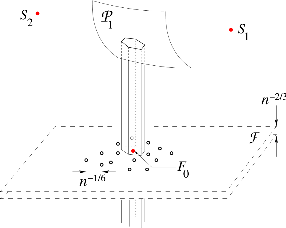
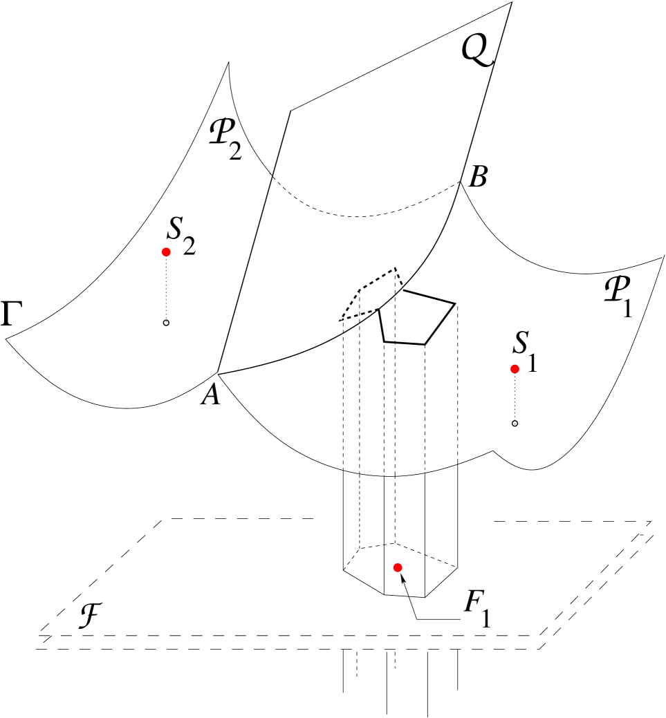
Figure 1: Both figures show the plane ${\cal F}$ containing the $n\gg 1$ neighbors of a many-faced central cell in a 3D Poisson-Voronoi diagram. The central seed itself is located at a distance $R_{n}\sim n^{1/3}$ below the plane and is not shown. The second-neighbor seeds, of which $\mathbf{S}_{1}$ and $\mathbf{S}_{2}$ are examples, have a density $\rho$. Left: The typical prism shaped first-neighbor Voronoi cell of seed $\mathbf{F}_{0}$ has its upper end face in contact with a single second neigbor cell. It is therefore eight-faced. Right: The exceptional first-neighbor Voronoi cell of seed $\mathbf{F}_{1}$ has its upper end in contact with two  second-neighbor cells, so that it is nine-faced. Figures taken from Ref. [9].

3 The Poisson-Möbius diagram ${\cal G}$

3.1 Definition of ${\cal G}$

We begin by considering a rectangular box $[-L,L]^{2}\times[0,L]$ whose volume we denote by $V=4L^{3}$. Let the seeds in this box be located at $\mathbf{S}_{1},\mathbf{S}_{2},\ldots,\mathbf{S}_{N}$ with $N$ such that $N/V=\rho$. We will at some convenient point let $L\to\infty$ at fixed $\rho$, so that the box becomes $\mathbb{R}^{3}_{+}$ and the $\mathbf{S}_{i}$ become Poisson distributed. We set $\mathbf{S}_{i}=(x_{i},y_{i},z_{i})$.

The surface $z=P_{i}(x,y)$ given by

$$P_{i}(x,y)=\frac{z_{i}}{2}\left(1+\frac{(x-x_{i})^{2}+(y-y_{i})^{2}}{z_{i}^{2}}\right)$$ (3.1)

is a paraboloid of revolution of focus $\mathbf{S}_{i}$ and axis perpendicular to the $xy$ plane. It separates $\mathbb{R}^{3}_{+}$ into a region containing all points closer to the $xy$ plane than to seed $\mathbf{S}_{i}$, and its complement.

Let $z=\Gamma(x,y)$ be the surface that separates the upper half-space $\mathbb{R}^{3}_{+}$ into a region of points closer to the $xy$ plane than to any  of the seeds, and its complement. Then $\Gamma(x,y)$ is built up out of piecewise paraboloidal surface elements ${\cal P}_{i}$ lying on the $P_{i}$. Only paraboloids $P_{i}$ associated with seeds $\mathbf{S}_{i}$ sufficiently close to the $xy$ plane will contribute surface elements. The arcs along which the surface elements of $\Gamma$ join will be referred to as ‘joints’.

The intersection of two arbitrary paraboloids $P_{1}$ and $P_{2}$ is an ellipse located in the plane that perpendicularly bisects the vector $\mathbf{S}_{1}-\mathbf{S}_{2}$ connecting the two foci. It is a remarkable but easily shown property that the projection of this ellipse onto the $xy$ plane is a circle. It follows that the joints are arcs of ellipses and that their projections onto the $xy$ plane constitute a planar diagram, to be called ${\cal G}$, whose edges are circular arcs. The diagram ${\cal G}$ divides the plane into cells $j$ each of which is associated with a specific seed $\mathbf{S}_{j}$. A snapshot of such a diagram is shown in Fig. 2. All vertices are trivalent, but not all edges end in vertices: some form full circles. Cells may not be convex; they may not be simply connected and may even be disconnected. The projection $\mathbf{s}_{j}=(x_{j},y_{j})$ of $\mathbf{S}_{j}$ may or may not be in cell $j$.

Diagrams whose edges are circular arcs (and their higher dimensional generalizations) have been called Möbius  diagrams by Boissonnat et al. [13], since they constitute an ensemble that is invariant under Möbius transformations. In the present case where the seeds are Poisson distributed, it seems appropriate to call ${\cal G}$ a Poisson-Möbius  diagram. This diagram is a random object and, since the seed density $\rho$ may be scaled away, it does not depend on any parameter. There are many interesting questions that one may ask about it.

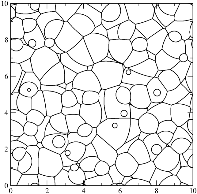
Figure 2: Poisson-Möbius diagram ${\cal G}$ obtained by projecting the surface elements ${\cal P}_{j}$ that constitute the surface $\Gamma$ [see section 3.1] onto the $xy$ plane.

3.2 Connection to weighted Voronoi diagrams

For a given point $\mathbf{r}=(x,y)$ in the $xy$ plane one may ask to which cell $j$ it belongs. This is obviously the cell of seed $\mathbf{S}_{j_{\rm min}}$ whose paraboloid is lower than all the others at $\mathbf{r}$, that is,

$$j_{\rm min}={\rm arg\,min}_{j}\,P_{j}(\mathbf{r}).$$ (3.2)

We may rephrase this as a two-dimensional problem in the following way. We refer to the projection $\mathbf{s}_{i}=(x_{i},y_{i})$ of seed $\mathbf{S}_{i}$ as a two-dimensional seed. Then $\mathbf{r}$ is in the cell of the seed $\mathbf{s}_{j_{\rm min}}$ to which it is closest according to the modified distance function given by

$${\rm dist}(\mathbf{r},\mathbf{s}_{i})=z_{i}^{-1}|\mathbf{r}-\mathbf{s}_{i}|^{2}+z_{i}\,,$$ (3.3)

in which the $z_{i}$ are now interpreted a ‘weights’ that render the two-dimensional seed $\mathbf{s}_{i}$ inequivalent. The diagram ${\cal G}$ hence appears as an ordinary two-dimensional Voronoi diagram but with the Euclidean distance replaced by the modified expression (3.3) that weights the seeds.

Weighted Voronoi diagrams with a variety of distance functions have been considered since many decades, often motivated by practical applications (see e.g. Ref. [14]). Okabe et al. [1] discuss the state of the art of weighted Voronoi diagrams up to the year 2000. Shortly after that, Boissonnat and Karavelas [15] introduced the distance function

$${\rm dist}(\mathbf{r},\mathbf{s}_{i})=\lambda_{i}|\mathbf{r}_{i}-\mathbf{s}_{i}|^{2}-\mu_{i}\,,$$ (3.4)

where $\lambda_{i}$ and $\mu_{i}$ are weights. With this distance definition (3.4) it is easily shown that the edge separating the Voronoi cells of two seeds at $\mathbf{s}_{i}$ and $\mathbf{s}_{j}$ is an arc of a circle. The distance function of this paper, Eq. (3.3), is the special case of Eq. (3.4) with $\lambda_{i}=z_{i}^{-1}$ and $\mu_{i}=-z_{i}$.

The literature that deals with weighted Voronoi diagrams is often concerned either with fairly abstract mathematical properties; or with questions about the computational complexity of algorithms that construct a diagram from a given set of $N$ seeds and their weights. Here we address the subject from a statistical point of view, the diagram ${\cal G}$ defined above being stochastic. Various of its properties may be calculated. Below we will focus directly on the particular property that we need, viz. the total edge length $\lambda$ per unit area.

3.3 Edge length per unit area in ${\cal G}$

The question of interest to us here is: what is the total length $\lambda$ of the edges of ${\cal G}$ per unit area? For the two-dimensional Poisson-Voronoi  diagram of seed density $\rho_{2}$ the value $\lambda=2\rho_{2}^{1/2}$ is part of a long list of exactly established results. This quantity has the dimension of a length per area, that is, of an inverse length. Hence in the present case we should have $\lambda=c\rho^{1/3}$ and the nontrivial part of the problem is to calculate the dimensionless coefficient $c$.

Let us consider the infinitesimal line segment connecting $(0,0)$ to $(\Delta x,0)$. We ask for the probability, to be called $p(\theta)\Delta x\Delta\theta$, that this line segment be intersected by an edge of ${\cal G}$ that has an orientation (by which we will mean an angle with the $y$ axis) in $[\theta,\theta+\Delta\theta]$ (see Fig. 3). If we take the line segment to be the side of a parallelogram of height $\Delta w$ in the $xy$ plane, we see that the edge length of ${\cal G}$ inside this parallelogram equals $\Delta\ell(\theta)=\Delta w/\cos\theta$. Therefore the expected edge length crossing a surface area $\Delta A=\Delta x\Delta w$ at an angle $\theta$ is

$$\langle\Delta\ell(\theta)\rangle = p(\theta)\Delta\theta\Delta x\cdot\frac{\Delta w}{\cos\theta}$$ (3.5)

$$= \frac{p(\theta)}{\cos\theta}\,\Delta\theta\Delta A.$$

The total expected edge length $\lambda\Delta A$ crossing a surface element $\Delta A$ is equal to the integral of (3.5) on $\theta$, whence

$$\lambda=\int_{-\pi/2}^{\pi/2}{\rm d}\theta\,\frac{p(\theta)}{\cos\theta}\,.$$ (3.6)

We will now calculate $p(\theta)$.

Figure 3: An element (heavy line) of an edge of the diagram ${\cal G}$ of circular arcs intersecting a line segment of length $\Delta x$ on the $x$ axis. It contributes a length $\Delta\ell=\Delta w/cos\theta$ to the parallelogrammatic area $\Delta A=\Delta x\Delta w$.

The probability for two arbitrary paraboloids $P_{j}$ and $P_{k}$ to contribute to the surface $\Gamma$ a joint whose projection crosses the above infinitesimal line segment is also the probability that the joint between $P_{j}$ and $P_{k}$ crosses the strip of zero thickness and infinitesimal width defined by $0<x<\Delta x$, $y=0$, and $z>0$, which in turn is $\binom{N}{2}$ times the probability that the joint between the paraboloids $P_{1}$ and $P_{2}$ does so. Let the joint intersect the $xz$ plane in $(x_{12},0,z_{12})$ and let its projection onto the $xy$ plane intersect the $x$ axis at an orientation $\theta_{12}$. Hence, averaging over all seed configurations, we have

$$p(\theta)\Delta\theta\Delta x= \frac{N(N-1)}{2V^{N}}\int_{-L}^{L}{\rm d}x_{1}{\rm d}x_{2}{\rm d}y_{1}{\rm d}y_{2}\int_{0}^{L}{\rm d}z_{1}{\rm d}z_{2}\,\,\chi_{12}(x_{12},\theta_{12})$$ (3.7)

$$\times\int_{-L}^{L}\prod_{i=3}^{N}{\rm d}x_{i}{\rm d}y_{i}\int_{0}^{L}\prod_{i=3}^{N}{\rm d}z_{i}\prod_{i=3}^{N}\Theta_{i}(z_{12}),$$

in which $z_{12}$ is the common value of $P_{1}$ and $P_{2}$ at the point of intersection, that is $z_{12}=P_{j}(x_{12},0)$ for $j=1,2$; the Heaviside function $\Theta_{i}$ imposes that the $i$th paraboloid does not intersect the strip in a point lower than $z_{12}$, that is

$$\Theta_{i}(z_{12})=\left\{\begin{array}[]{ll}1&\mbox{if }P_{i}(x_{jk},0)>z_{jk}\,,\\[5.69054pt] 0&\mbox{otherwise};\end{array}\right.$$ (3.8)

and

$$\chi_{12}(x_{12},\theta_{12})=\left\{\begin{array}[]{ll}1&\mbox{if }0<x_{12}<\Delta x\mbox{ and }\theta<\theta_{12}<\theta+\Delta\theta,\\[5.69054pt] 0&\mbox{otherwise}.\end{array}\right.$$ (3.9)

The $N-2$ triple integrals on $(x_{i},y_{i},z_{i})$ for $i=3,\ldots,N$ may be carried out independently for each $i$. The factor $\Theta_{i}$ imposes that the integrand vanishes if $(x_{i},y_{i},z_{i})$ is inside the sphere of radius $z_{12}$ around $(x_{12},0,z_{12})$. Hence the result of these integrations is $(V-\tfrac{4}{3}\pi z_{12}^{3})^{N-2}$ which in the limit $L\to\infty$ becomes $V^{N-2}\exp(-\tfrac{4}{3}\pi z_{12}^{3}\rho)$. Upon taking the limit $L\to\infty$ in (3.7) we get

$$p(\theta)\Delta\theta\Delta x=\frac{\rho^{2}}{2}\int_{-\infty}^{\infty}{\rm d}x_{1}{\rm d}x_{2}{\rm d}y_{1}{\rm d}y_{2}\int_{0}^{\infty}{\rm d}z_{1}{\rm d}z_{2}\,\,\chi_{12}(x_{12},\theta_{12})\exp(-\tfrac{4}{3}\pi z_{12}^{3}\rho).$$ (3.10)

Near the origin of the $xy$ plane the paraboloids $P_{j}(x,y)$ with $j=1,2$ may be linearized according to

$$P_{j}(x,y)=r_{j}+s_{j}x+t_{j}y+{\cal O}(x^{2},y^{2})$$ (3.11)

where

$$r_{j}=\frac{z_{j}}{2}\Big{(}1+\frac{x_{j}^{2}+y_{j}^{2}}{z_{j}^{2}}\Big{)},\qquad s_{j}=-\frac{x_{j}}{z_{j}},\qquad t_{j}=-\frac{y_{j}}{z_{j}}\,.$$ (3.12)

We now transform from $(x_{j},y_{j},z_{j})$ to new variables of integration $(r_{j},s_{j},t_{j})$, where $j=1,2$. The Jacobian is

$$\frac{\partial(r_{j},s_{j},t_{j})}{\partial(x_{j},y_{j},z_{j})}=\frac{(1+s_{j}^{2}+t_{j}^{2})^{3}}{8r_{j}^{2}}\,.$$ (3.13)

With this transformation Eq. (3.10) becomes

$$p(\theta)\Delta\theta\Delta x = 32\rho^{2}\int_{-\infty}^{\infty}\frac{{\rm d}s_{1}{\rm d}s_{2}{\rm d}t_{1}{\rm d}t_{2}}{(1+s_{1}^{2}+t_{1}^{2})^{3}(1+s_{2}^{2}+t_{2}^{2})^{3}}$$ (3.14)

$$\times\int_{0}^{\infty}{\rm d}r_{1}{\rm d}r_{2}\,r_{1}^{2}r_{2}^{2}\,\chi_{12}(x_{12},\theta_{12})\exp(-\tfrac{4}{3}\pi z_{12}^{3}\rho)$$

in which $\chi_{12}$ couples the variables with indices $1$ and $2$. The coordinate $x_{12}$ of the point of intersection is the solution of $P_{1}(x_{12},0)=P_{2}(x_{12},0)$ which upon linearization gives

$$x_{12}=-\frac{r_{2}-r_{1}}{s_{2}-s_{1}}\,.$$ (3.15)

Using (3.15) we can rewrite the condition $0<x_{12}<\Delta x$ as

$$r_{1}-\Delta x(s_{2}-s_{1})<r_{2}<r_{1}\,,\qquad s_{2}>s_{1}\,,$$

$$r_{1}<r_{2}<r_{1}+\Delta x(s_{1}-s_{2}),\qquad s_{1}>s_{2}\,.$$ (3.16)

In both cases $r_{2}$ is integrated on an infinitesimal interval of length $|s_{1}-s_{2}|\Delta x$ located at $r_{1}$. This takes account of the condition on $x_{12}$ implied by $\chi_{12}(\Delta x,\Delta\theta)$ and shows furthermore that $z_{12}=r_{1}+{\cal O}(\Delta x)=r_{2}+{\cal O}(\Delta x)$. Hence Eq. (3.14) becomes, after we divide it by $\Delta x$ and scale $\rho$ out of the integrand,

$$p(\theta)\Delta\theta = 32I_{0}\rho^{\frac{1}{3}}\int_{-\infty}^{\infty}{\rm d}s_{1}{\rm d}s_{2}{\rm d}t_{1}{\rm d}t_{2}\,\frac{|s_{1}-s_{2}|}{(1+s_{1}^{2}+t_{1}^{2})^{3}(1+s_{2}^{2}+t_{2}^{2})^{3}}\,\chi_{12}^{\rm ang}(\theta_{12})$$

in which

$$I_{0}=\int_{0}^{\infty}{\rm d}r\,r^{4}\,\exp(-\tfrac{4}{3}\pi r^{3})=\tfrac{2}{9}(\tfrac{4}{3}\pi)^{-\frac{5}{3}}\Gamma(\tfrac{2}{3})$$ (3.18)

and where $\chi_{12}^{\rm ang}(\theta_{12})$ imposes the remaining condition $\theta<\theta_{12}<\theta+\Delta\theta$. The point of intersection $(x_{12},0,z_{12})$ being known, we now look for the line of intersection by setting $x=x_{12}+\delta x$ and $y=\delta y$. Substituting in (3.11) and eliminating $r_{1}=r_{2}$ we find that $s_{1}\delta x+t_{1}\delta y=s_{2}\delta x+t_{2}\delta y$, whence

$$\tan\theta_{12}=\frac{\delta x}{\delta y}=-\frac{t_{2}-t_{1}}{s_{2}-s_{1}}\,.$$ (3.19)

We will now perform the integration on $t_{1}$ in (LABEL:xptheta4). Reasoning in the same way as for the integration on $r_{2}$ we find from (3.19) and the condition imposed by $\chi_{12}^{\rm ang}$ that this integration has nonvanishing contributions only for $t_{1}$ in an infinitesimal interval located at $t_{2}+(s_{2}-s_{1})\tan\theta\equiv t_{1}(\theta)$ and having a length $|s_{1}-s_{2}|\Delta\theta/\cos^{2}\theta=\mbox{sgn}(s_{2}-s_{1})\frac{{\rm d}t_{1}}{{\rm d}\theta}\Delta\theta$. This observation allows us to write Eq. (LABEL:xptheta4), after dividing by $\Delta\theta$, as

$$p(\theta)=32I_{0}\rho^{\frac{1}{3}}\int_{-\infty}^{\infty}{\rm d}s_{1}{\rm d}s_{2}\frac{{\rm d}t_{1}}{{\rm d}\theta}\,{\rm d}t_{2}\,\frac{s_{2}-s_{1}}{(1+s_{1}^{2}+t_{1}^{2}(\theta))^{3}(1+s_{2}^{2}+t_{2}^{2})^{3}}\,.$$ (3.20)

We substitute Eq. (3.20) in Eq. (3.6). The integral on $\theta$ in the resulting expression is easily reconverted into one on $t_{1}$ by means of the relation

$$\int_{-\pi/2}^{\pi/2}{\rm d}\theta\,\frac{{\rm d}t_{1}}{{\rm d}\theta}=\int_{-\infty}^{\infty}{\rm d}t_{1}\,\mbox{sgn}(s_{2}-s_{1}).$$ (3.21)

We use furthermore that $|s_{2}-s_{1}|/\cos\theta$ is the distance between the points $(s_{1},t_{1})$ and $(s_{2},t_{2})$ and find for $\lambda$ the expression

$$\lambda=32\,I_{0}\rho^{\frac{1}{3}}\int_{-\infty}^{\infty}{\rm d}s_{1}{\rm d}s_{2}{\rm d}t_{1}{\rm d}t_{2}\,\frac{|s_{2}-s_{1}|}{(1+s_{1}^{2}+t_{1}^{2})^{3}(1+s_{2}^{2}+t_{2}^{2})^{3}}\,.$$ (3.22)

We may cast this integral into a more elegant form by passing to the polar coordinates

$$(s_{j},t_{j})=\rho_{j}(\cos\phi_{j},\sin\phi_{j}),\qquad j=1,2.$$ (3.23)

The integrand appears to depend only on the $\rho_{j}$ and on the angle difference $\phi\equiv\phi_{1}-\phi_{2}$. Regrouping factors we may write the final result as

$$\lambda=\left(\tfrac{4}{3}\pi\right)^{\frac{1}{3}}\Gamma\left(\tfrac{2}{3}\right)I_{1}\,\rho^{\frac{1}{3}}$$ (3.24)

in which

$$I_{1}=\int_{0}^{\infty}\frac{4\rho_{1}\,{\rm d}\rho_{1}}{(1+\rho_{1}^{2})^{3}}\int_{0}^{\infty}\frac{4\rho_{2}\,{\rm d}\rho_{2}}{(1+\rho_{2}^{2})^{3}}\int_{0}^{\pi}\frac{{\rm d}\phi}{\pi}\sqrt{\rho_{1}^{2}+\rho_{2}^{2}-2\rho_{1}\rho_{2}\cos\phi}.$$ (3.25)

It is, as it should, independent of the orientation of the initially chosen line segment. In terms of the variables of integration $q=\phi/\pi$ and $u_{j}=r_{j}^{2}/(1+r_{j}^{2})^{2}$ (where $j=1,2$) Eq. (3.25) becomes an integral on the unit cube $[0,1]^{3}$. Numerical evaluation gives $I_{1}=1.1566$. Putting in the other numbers we find from Eq. (3.24) that

$$\lambda=c\,\rho^{\frac{1}{3}},\qquad c=2.525,$$ (3.26)

which is the final answer for $\lambda$.

4 Monte Carlo simulation of ${\cal G}$

To check the result (3.26) we performed a Monte Carlo simulation using a poor man’s algorithm sufficient for the present purpose. We considered a volume $[0,L]^{2}\times[0,M]$, took periodic boundary conditions in the $x$ and $y$ directions, and chose $1000\times 1000$ grid points $(\tilde{x},\tilde{y})$ in the $xy$ plane. Initially all grid points get assigned a hight value $g(\tilde{x},\tilde{y})=M/2$ and an integer index $n(\tilde{x},\tilde{y})=0$. For $i=1,2,3,\ldots$ we generated seeds $(x_{i},y_{i},z_{i})$ with a scaled density $\rho=1$ such that $z_{1}<z_{2}<z_{3}<\ldots$. After the generation of each seed $i$ we reassigned to every grid point $(\tilde{x},\tilde{y})$ the value $g(\tilde{x},\tilde{y})=P_{i}(\tilde{x},\tilde{y})$ as long as this value was less than the current value of $g(\tilde{x},\tilde{y})$; and in that case replaced the current index $n(\tilde{x},\tilde{y})=0$ by $i$ (indicating that $(\tilde{x},\tilde{y})$ is provisionnaly in the cell of seed $i$). It is easily verified that this reassignment requires considering only the grid points within a radius $M(z_{i}-M)$ around $(x_{i},y_{i})$. As $i$ increases, a value $z_{i}>M$ will be reached. Then, provided that at that moment the condition $g(\tilde{x},\tilde{y})<M/2$ is fulfilled for all $(\tilde{x},\tilde{y})$, seeds with higher $z_{i}$ cannot any further modify the function $g(\tilde{x},\tilde{y})$; the construction process ends and $g(\tilde{x},\tilde{y})$ is equal to the surface $\Gamma(\tilde{x},\tilde{y})$. The value of $M$ should be chosen large enough so that this latter condition is satisfied with overwhelming probability.

The cell boundaries may be determined by comparing the final $n$ values of each pair of neighboring grid points, which gives rise to structures as shown in Fig. 2. To determine the total length of the cell boundaries, we determined the total length of their projections onto the $x$ and $y$ axes and, knowing that statistically all angles of the line segments have the same probability, multiplied the total projected length by $\pi/4$. We obtained $\lambda=2.512\pm 0.003$ as the result of an average over 3000 samples with $L=10$ and $M=4$. We consider this agreement as quite satisfactory given the resolution of the grid and the possibility of finite size effects.

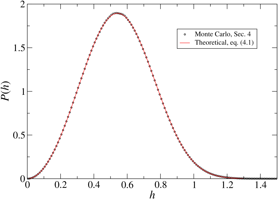
Figure 4: Height distribution $P(h)$ of the surface $\Gamma$ above the $xy$ plane. Black circles are our Monte Carlo data, the red solid curve is our theoretical prediction.

As a further check we considered the distribution $P(h)$ of the height $h$ of surface $\Gamma$ above the $xy$ plane. This distribution is easily calculated by the methods of section 3, but there is a simpler argument: $P(h)\Delta h$ it is the probability that a sphere of diameter $h$ tangent to the $xy$ plane be empty and that there be a seed in the shell of width $\Delta h$ that envelopes it. Hence

$$P(h)=4\pi h^{2}\,{\rm e}^{-\frac{4}{3}\pi h^{3}}.$$ (4.1)

In Fig. 4 we show our Monte Carlo data for $P(h)$. The agreement is perfect. It follows that the average surface height is given by $\langle h\rangle=\int_{0}^{\infty}{\rm d}h\,hP(h)=0.553\,96$. Several other surface properties may be calculated exactly, but we will leave this for future work.

5 Application to $m_{n}(3)$

5.1 The coefficient $k_{1}$

We will now use the result of section 3.3 to determine the conditional facedness $m_{n}(3)$ of the three-dimensional Voronoi cell in the limit of large $n$. As explained in section 2 we should consider the superposition in the $xy$ plane (i.e. plane ${\cal F}$ in Fig. 1) of the Poisson-Möbius diagram ${\cal G}$ with two-dimensional system of Voronoi cells generated by the first-neighbor seeds. This system is very fine-mazed, the typical linear size of a cell being $\sim n^{-1/6}$. We will refer to them as ‘small cells’ in order to distinguish them from the superposed Poisson-Möbius cells. The fraction of small cells intersected by the edges of ${\cal G}$ was called $f_{9}=k_{1}n^{-1/6}+\ldots$ in section 2, and we are now in a position to estimate the coefficient $k_{1}$. For large $n$ the only property of ${\cal G}$ that matters is its total length $\lambda$ per unit surface that we have just calculated; at the scale of the small maze the circular nature of the edges of ${\cal G}$ plays no role.

The $n$ first neighbor seeds are located on a spherical surface of radius $R_{n}$ determined by $n=\frac{4}{3}\pi R_{n}^{3}\rho$. The average area $a$ of a small cell therefore is

$$a=(4\pi R_{n}^{2})/(\tfrac{4}{3}\pi R_{n}^{3}\rho)=4\pi(\tfrac{4}{3}\pi\rho)^{-\frac{2}{3}}n^{-\frac{1}{3}}.$$ (5.1)

The small cells, although not Poisson, are nevertheless convex and in the limit $n\to\infty$ a convex cell $\ell$ of perimeter $p_{\ell}$ has a probability $(\lambda/\pi)p_{\ell}$ to be intersected by a line of ${\cal G}$. The total number $n_{\rm int}$ of small intersected cells will therefore be $n_{\rm int}=(\lambda/\pi)\sum_{\ell}p_{\ell}$. We will write $p_{\ell}=a^{\frac{1}{2}}\bar{p}_{\ell}$ in which $\bar{p}_{\ell}$ is the dimensionless perimeter of cell $\ell$ when the average cell area is scaled up to unity. Hence we get for $f_{9}=n_{\rm int}/n=(\lambda/\pi)\sum_{\ell}\bar{p}_{\ell}$ the expression

$$f_{9}=\frac{\lambda}{\pi}\,a^{\frac{1}{2}}\bar{p}$$ (5.2)

in which $\bar{p}$ denotes the average dimensionless perimeter of a scaled cell. With the aid of (3.26) for $\lambda$ and (5.1) for $a$ this yields a numerical constant

$$k_{1}=\lim_{n\to\infty}n^{\frac{1}{6}}f_{9}=\frac{c}{\pi}\,(36\pi)^{\frac{1}{6}}\,\bar{p}.$$ (5.3)

The seeds $\mathbf{F}_{j}$ of the small cells are not Poisson distributed (there is strong indication that in fact they repel each other [9]), but we ignore their exact statistics and in particular their average cell perimeter. We will therefore use at this point the best possible estimate for $\bar{p}$, which varies only moderately between different cellular structures. Noting that a two-dimensional Poisson-Voronoi diagram has $\bar{p}=4$ and a regular hexagonal lattice has $\bar{p}=2^{\frac{3}{2}}3^{\frac{1}{4}}=3.722$, we may quite reasonably estimate that in our case $\bar{p}=3.85\pm 0.15$. Substituting in (5.3) also the numerical value of $c$ from (3.26) we obtain $k_{1}=6.8\pm 0.3$, which is our final result for $k_{1}$. Upon combining it with Eq. (1.2) we find that the series for $m_{n}$ when truncated after its second term takes the form

$$m_{n}(3)=8+6.8\,n^{-\frac{1}{6}}.$$ (5.4)

We consider this expression as ‘semi-exact’, a qualification to be understood in the context of the preceding discussion and to be commented upon in our conclusion.

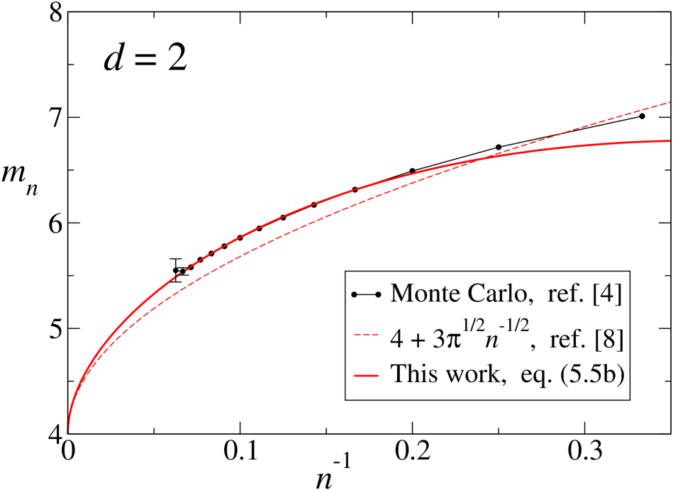
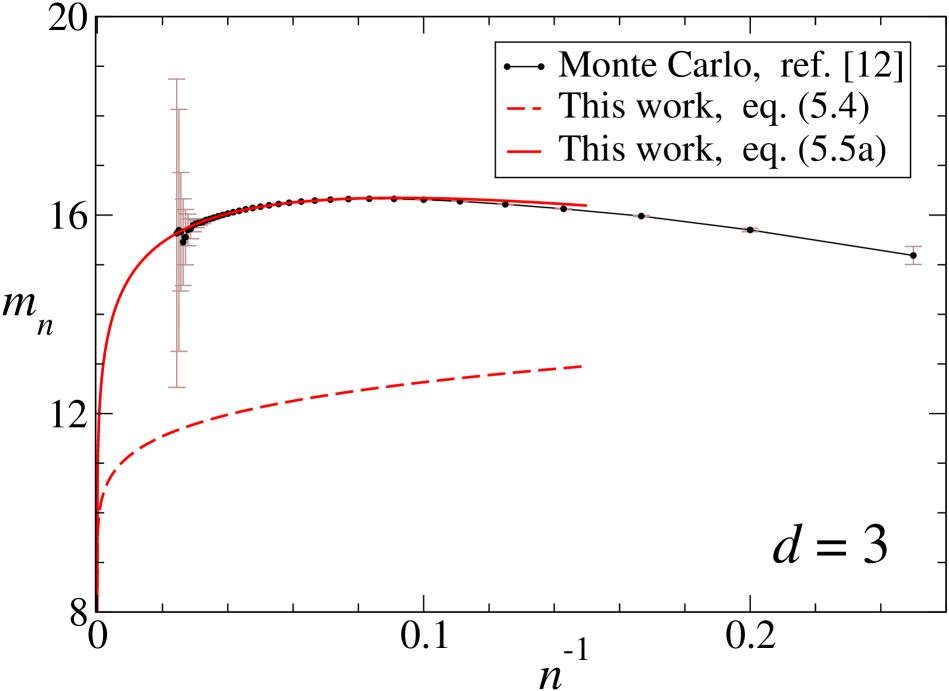
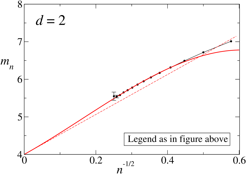
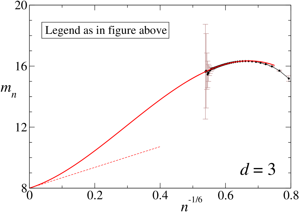
Figure 5: Conditional sidedness $m_{n}$ in dimensions $d=2$ (left column) and $d=3$ (right column). The top row shows the curves as a function of $n^{-1}$; they would be linear if Aboav’s law held. The bottom row shows them as a function of $n^{-1/2}$ and $n^{-1/6}$, respectively; according to our theory, they are asymptotically linear in these variables. See text for further comments.

5.2 Comparison

We now compare Eq. (5.4) to the data obtained by Lazar et et al. [12]. In Fig. 5 we present in the top right figure the new three-dimensional $m_{n}$ simulation data due to Lazar et et al. [12] as a function of $n^{-1}$ (black dots with error bars in brown). In the top left corner we show for comparison the two-dimensional data of Ref. [4]. The three-dimensional data cover the range $4\leq n\leq 41$, the statistical uncertainty increasing strongly for the higher values of $n$.

Sidetracking a little we point out that one of the discoveries of Ref. [12] was that the 3D curve has a maximum, contrary to the one in 2D, namely at $n=12$; we think that an intuition about why there is such a maximum would be welcome, but do not have any at present. It is furthermore striking that all 3D data points are in the range $15.1<m_{n}<16.4$, that is, their absolute range of variation is smaller than that of the 2D data. Put concisely, “in dimension $d=3$ a neighbor cell resembles the central cell more than in $d=2$.” It is also clear, finally, that there is still a big gap between the $m_{n}$ data at the highest $n$ values (which are around $\approx 15.5$) and the asymptotic value predicted by us [9] to be $m_{\infty}=8$.

We now compare these Monte Carlo data to our theory. The dashed red curve in the $d=3$ figure represents Eq. (1.2) obtained above, the one in $d=2$ the first two terms of Eq. (1.1) taken from Ref. [8]. In both dimensions the asymptotic expansions truncated after two terms stay below the numerical data, however in the three-dimensional case much more so than in two dimensions.

The same curves are shown in the two bottom figures of Fig. 5 as a functions of $n^{-1/2}$ and of $n^{-1/6}$ in dimensions $d=2$ and $d=3$, respectively, and should in this representation be linear in the origin, that is, near the points $(4,0)$ and $(8,0)$, respectively. Qualitative similarities between the two-and three-dimensional situations may indeed be observed; e.g., in both cases the predicted asymptotic slope (dashed red lime) is too small and the Monte Carlo data, if they are going to join the asymptotic slope, must do so through a slight upward curvature. However, whereas asymptotic linear behavior is certainly suggested in $d=2$, it again appears that in $d=3$ the gap between the the simulation regime and the asymptotic limit is still considerable.

5.3 Fits

It has become a habit in this field to exhibit data fits, of which Aboav’s law (with two free parameters) has been only the simplest one. Yielding to this tradition we fit the data of Ref. [12] under the constraint of the asymptotic behavior derived above. That is, we will suppose for $m_{n}(3)$ an expansion in powers of $n^{-\frac{1}{6}}$ and analogously for $m_{n}(2)$ one in powers of $n^{-\frac{1}{2}}$ and extend the known series, (5.4) and (1.1), respectively, each with two more terms whose coefficients we will adjust. We optimize the value and the derivative of the fit in a small range where $n$ is as large as possible while (in the bottom row of Fig. 5) the Monte Carlo data are linear and the error bars are still small. In practice this was the range $0.57\lesssim n^{-\frac{1}{6}}\lesssim 0.59$ for $d=3$ and $0.27\lesssim n^{-\frac{1}{2}}\lesssim 0.32$ for $d=2$. We are led to

$$m_{n}(3)=8+6.8\,n^{-\frac{1}{6}}+35.23\,n^{-\frac{1}{3}}-39.98\,n^{-\frac{1}{2}},\\$$ (5.5a)

$$m_{n}(2)=4+3\pi^{\frac{1}{2}}n^{-\frac{1}{2}}+5.1\,n^{-1}-10.4\,n^{-\frac{3}{2}}.$$ (5.5b)

In both $d=3$ and $d=2$ the coefficient of the third term is positive and the one of the fourth term negative. In Fig. 5 we have represented Eqs. (5.5) by the solid red curves. These provide an excellent fit for large $n$ but, by construction, deviate from the data at low values of $n$.

In Ref. [8] a series similar to (5.5b) was constructed on the basis of fitting the two-dimensional data over the full range; this fit leads to a third and fourth coefficient different from those obtained here. A similar full-range fit of the three-dimensional data carried out in Ref. [12] and using $k_{1}$, $k_{2}$ and $k_{3}$ as free parameters led to a series similar to (5.5a) but again with different coefficients.

We of course do not imply that these fitted coefficients have a relation to those, unknown, of the asymptotic series; the latter are certainly very hard to calculate beyond the term $k_{1}$ we found in this paper and beyond the coefficient $3\pi^{\frac{1}{2}}$ found for $d=2$ in Ref. [8]. There is moreover no guarantee that the true higher order terms in the asymptotic expansion would improve the agreement with the Monte Carlo data: the expansion may well be divergent. Therefore these fitted curves are, if anything, our best guesses of what $m_{n}$ looks like for higher values of $n$. Simulations to test these curves would require more computer time or cleverer algorithms.

6 Conclusion

Prompted by the recent high precision simulation data of Lazar et al. on three-dimensional Poisson-Voronoi cells we have determined the coefficient $k_{1}$ in the asymptotic expansion of the conditional sidedness, $m_{n}(3)=8+k_{1}n^{-1/6}+\ldots$, for $n\to\infty$.

As a problem within the problem, the calculation requires the study of an auxiliary two-dimensional diagram that we have termed Poisson-Möbius diagram; it is part of a class of circular arc diagrams studied in the literature and is of interest for its own sake. For this diagram we have performed a fully exact calculation of the the edge length $\lambda$ per unit surface, which is a prerequisite for the coefficient $k_{1}$.

The calculation of $k_{1}$ itself rests on the hypotheses of Ref. [9], which amount to assuming that various effects that are being neglected, are of higher order in the expansion variable $n^{-1/6}$. Finally, error bars appear due to our ignorance of the arrangement of the first order neighbor cells on their surface.

We have compared our asymptotic expansion for $m_{n}(3)$ to the Monte Carlo data and concluded that in dimension $d=3$ the regime where simulation is possible is still far from the asymptotic limit. We have presented fits subject to the asymptotic constraint, which must be considered as our best guesses for the large $n$ behavior given the knowledge we have today.

References

- [1] A. Okabe, B. Boots, K. Sugihara, and S.N. Chiu, Spatial tessellations: concepts and applications of Voronoi diagrams, second edition (John Wiley & Sons Ltd., Chichester, 2000).
- [2] J.L. Meijering, Philips Research Reports 8, 270 (1953).
- [3] D.A. Aboav, Metallography 3, 383 (1970).
-
[4]
K.A. Brakke, unpublished. Available on
http://www.susqu.edu/brakke/papers/voronoi.htm - [5] H.J. Hilhorst, J. Stat. Mech. L02003 (2005).
- [6] H.J. Hilhorst, J. Stat. Mech. P09005 (2005).
- [7] H.J. Hilhorst, J. Phys. A 40, 2615 (2007).
- [8] H.J. Hilhorst, J. Phys. A 39, 7227 (2006).
- [9] H.J. Hilhorst, J. Stat. Mech. P08003 (2009).
- [10] S. Kumar, S.K. Kurtz, J.R. Banavar, and M.G. Sharma, J. Stat. Phys. 67, 523 (1992).
- [11] M.A. Fortes, Phil. Mag. Lett. 68, 69 (1993).
- [12] E.A. Lazar, J.K. Mason, R.D. MacPherson, D.J. Srolovitz, Phys. Rev. E 88, 063309 (2013).
- [13] J.-D. Boissonnat, C. Wormser, and M. Yvinec, in: Effective Computational Geometry for Curves and Surfaces, J.-D. Boissonnat and M. Teillaud, Monique (Eds.), Springer (Berlin, 2006), p. 67-116.
- [14] F. Aurenhammer and H. Edelsbrunner, Pattern Recognition 17, 251 (1984).
- [15] J.-D. Boissonnat and M.I. Karavelas, SODA ’03: Proceedings of the Fourteenth Annual ACM-SIAM Symposium on Discrete Algorithms, (2003), p. 305-312.