Macroscopic optomechanics from displaced single-photon entanglement
Résumé
Displaced single-photon entanglement is a simple form of optical entanglement, obtained by sending a photon on a beamsplitter and subsequently applying a displacement operation. We show that it can generate, through a momentum transfer in the pulsed regime, an optomechanical entangled state involving macroscopically distinct mechanical components, even if the optomechanical system operates in the single-photon weak coupling regime. We discuss the experimental feasibility of this approach and show that it might open up a way for testing unconventional decoherence models.
pacs:
03.67.BgIntroduction
Can a macroscopic massive object be in a superposition of two well distinguishable positions? It has been argued that such superpositions undergo intrinsic decoherence, e.g. due to a non-linear stochastic classical field GRW86 ; Pearle90 ; Gisin89 or caused by superposition’s perturbation of spacetime Diosi89 ; Penrose96 . These decoherence mechanisms are different from conventional decoherence that occurs through entanglement with the environment Zurek03 and that has been nicely demonstrated in Brune96 ; Turchette00 ; Hackermueller04 ; Deleglise08 ; Myatt00 . In contrast, testing for unconventional decoherence models requires a combination of large masses and superpositions of states corresponding to well separated positions. Matter-wave interferometry with large clusters Nimmrichter11 or with submicron particles Romero-Isart11 is one possible route. Another approach is to manipulate states of motion of massive mechanical resonators, a fast moving field of research that has now succeeded in entering the quantum regime Oconnell10 ; Teufel11 ; Chan11 . In the framework of optically controlled mechanical devices Aspelmeyer13 , the proposals Bose97 ; Bose99 have the potential to create a superposition of mechanical states with a distance of the order of the mechanical zero-point fluctuation where the effects of unconventional decoherences might be observable Marshall03 ; Kleckner08 . However, this requires (i) to work in the single-photon strong coupling regime, (ii) a coupling rate at least of the order of the mechanical frequency so that the displacement induced by a single photon is larger than the mechanical zero point spread, (iii) to work in the resolved sideband regime where the mechanical frequency is larger than the cavity decay rate to allow ground state cooling. While (i) and (ii) can be relaxed, e.g. using nested interferometry Pepper12prl and (iii) can be circumvented by cooling e.g. via pulsed optomechanical interactions Vanner11 , the distance between the superposed states remains small, of the order of the mechanical ground state extension.
Here, we show how to create macroscopic optomechanical entanglement with relatively simple ingredients. Our proposal starts with an optical entangled state of the type involving two spatial modes and Concretely, this state is obtained by sending a single photon into a beamsplitter (with output modes and ) and by subsequently applying a phase-space displacement on . The displaced photons in then interact with a mechanical system through radiation pressure. If the interaction between and falls within the pulsed regime Cerrillo11 ; Vanner11 ; Wang11 where the pulse duration is much smaller than the mechanical period, the optical and mechanical modes entangle, Because and are well distinguishable in photon number, the mechanical components tr are well distinct in the phase space even in the weak coupling regime and if the coupling rate is smaller than the mechanical frequency. This relaxes the constraints on the initial cooling of the mechanical oscillator and makes our proposal well suited to test unconventional decoherence processes, as we show below.
Optomechanical entanglement

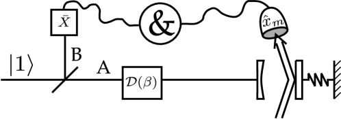
Consider an optomechanical cavity described by where is the angular frequency of the center of mass motion of the mechanical system, are the bosonic operators for the phononic (photonic) modes and for a Fabry-Perot cavity with a mechanically moving end mirror ( is the optical angular frequency, is the cavity length and M is the effective mass of the mechanical mode). The form of the optomechanical interaction, proportional to (where is the position operator, being the mechanical zero-point fluctuation amplitude) tells us that starting with a superposition of photonic components that are well distinguishable in photon number space, we can create a superposition of mechanical states corresponding to well distinct momenta. Displaced single-photon entanglement exhibits such a property Sekatski12 ; Sekatski13 and has the advantage of being easily prepared, see Fig. 1. It can be written as
| (1) |
where being the vacuum, the single photon Fock state foonotesinglet . stands for the displacement operator and can be implemented using an unbalanced beamsplitter and a coherent state Paris96 . Although the photon number distributions for and partially overlap (their variance is given by ), their mean photon numbers are separated by 2 Sekatski12 . (Here is considered real, as all along the paper). In other words, their distance in the photon number space is of the order of the square root of their size. This makes the state (1) macroscopic in the sense that its components can be distinguished without a microscopic resolution Sekatski13 .
Consider first the case where photons interact with the mechanical mode initially prepared in its motional ground state According to Bose97 , they induce a coherent displacement of the mechanical state whose amplitude varies periodically in time The first exponential term corresponds to the variation of the cavity length and is quadratic in the photon number because the mean position of the mechanical oscillator depends on the photon number. To avoid this non-linear behavior, we consider the pulsed regime where the interaction time is much smaller than the mechanical period (, c.f. below for the detailed conditions). Right after this interaction, the propagator has the simple form
and after a free evolution of duration the overall propagator can be written as
An initial state now evolves towards
where is a coherent state with a fixed amplitude and a periodic phase In other words, the photons kick the mechanical mode that gets an additional momentum at time ( is the initial mechanical momentum spread). The mechanical state then starts to rotate in phase space. It reaches a minimal position after then gets a momentum after and so on.
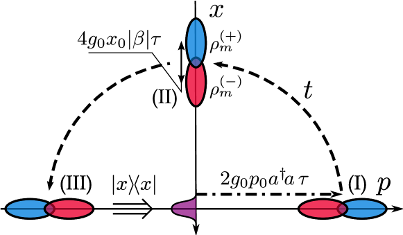
Let us now come back to the initial state (1). The pulse in enters the optomechnical cavity, the mechanical mode being in , as before. A time after the interaction, the state of the system is
| (2) | |||||
where are the probability amplitudes for having photons in
Since the mechanical mode entangles with the optical modes. Specifically, after the state (2) involves two mechanical states each having a variance in space and for which the mean position is separated by (see fig. 2). These two mechanical states can thus be distinguished with a detector having a resolution see below. For such a detector cannot resolve two phononic Fock states with and excitations (no microscopic resolution) and the entangled state (2) can fairly be defined as being macroscopic.
Macroscopic correlations
We now show how to demonstrate that the mechanical mode involves macroscopically distinct states .
More precisely, we show that and are correlated, i.e. when the state of B is projected into (), the mechanical mode is found in () a quarter of a mechanical period after the interaction, (c.f. Fig. 3) and that these correlations can be revealed without the need for a microscopic resolution. This is done by tracing out and by measuring the quadrature of and the mirror position. The latter can be realized following Vanner11 , by observing through a quadrature measurement the phase acquired by a strong, short light pulse reflected by the mechanical oscillator. We attribute the value () to a positive (negative) result of the quadrature measurement on and if the mirror is found to be shifted more to the left (right) with respect to its mean position . For an uncertainty on the measurement of the mirror position, the probability for having the same results is given by (for ) while the probability for having different results Therefore, the correlations between the outcomes (the probability for having correlated results minus the probability for having anti-correlated results) are given by
In the regime of interest even a coarse grained measurement with the resolution leads to substantial correlations This is a consequence of the macroscopic characteristic of the optomechanical state (2).
Testing unconventional decoherence models
Fig. 4 shows how to probe the effect of mirror decoherence. First, the mechanical position is measured at any time that is a multiple of half a mechanical period where no information is obtained about the state of Finding the mirror at the position projects the overall state into
| (3) | |||||
Actively controlling the relative length of paths and to get rid of the undesired phase term and subsequently applying leaves
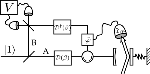
the optomechanical state in The modes and can then be combined on a beamsplitter and varying their relative phase leads to interference fringes, ideally with a unit visibility (Note here that from the values of the probabilities of detecting photons in A and in B, a lower bound on the negativity between and can be obtained through the approach presented in Chou05 .) Decoherence of the mirror operates as a weak measurement of the photon number on (see SM). Therefore, if the measurement of the mechanical position is delayed, more and more ”which path” information is revealed which decreases the visibility as the delay time increases. Importantly, different types of decoherence give rise to different behaviors of the visibility as the delay time increases. As particular examples, we compare conventional (environmental induced) decoherence with unconventional decoherence proposed by gravitationally induced collapse Diosi89 ; Penrose96 and by quantum gravity Ellis84 (see SM). For sufficiently large i.e. macroscopic entanglement, and small thermal dissipation we find an experimentally feasible parameter regime, in which the unconventional decoherence rates surpass the conventional ones, hence opening up the possibility for experimental tests (see below). Finally, note that the observed visibility is degraded if the mirror position is not accurately measured. A small imprecision would indeed introduce an additional phase on that prevents its re-displacement to the single photon level and degrades the quality of the interference between and Sekatski12 ; footnote_phase_dis . Quantitatively,
| (4) |
where
A high accuracy is thus required to observe high visibility and to see the effect of mirror decoherence.
Witnessing optomechanical entanglement
We can prove that the mirror is entangled with the optical modes from an entanglement witness which uses the values of and only (see SM). The witness is based on the following intuitive argument: since is a qubit, the only way for to be correlated to and for to be entangled with the joint system is that is entangled with Concretely, we can conclude about optomechanical entanglement if We emphasize that in contrast to the correlation measurement, the detection of entanglement requires a measurement of the mirror position with a very high accuracy (through ). We are retrieving what seems to be the essence of macro entangled states: although they involve components that can easily be distinguished without microscopic resolution, one needs detectors with a very high precision to reveal their quantum nature Sekatski13 .
Experimental feasibility
We now address the question of the experimental feasibility in detail. First, we require which allows one to observe significant correlations between and
To further guarantee a high visibility of the interference between and the system needs to operate in the linear regime. For a pulsed optomechanical interaction the non-linear response of the optomechanical system degrades the visibility of the interference pattern according to where footnote_phase . This undesired effect is thus negligible if The requirement of observing a high interference visibility also imposes the mirror position to be accurately estimated, c.f. eq. (4). It has been established in Vanner11 that the maximum accuracy is obtained by choosing an input drive with a duration The achievable precision then depends on its number of photons via and is thus high if The primary limitation for is the power that can be homodyned before photodetection begins to saturate. Assuming a saturation power of 10 mW results in To build up a proposal as simple as possible, we consider the case where a single local oscillator with a controllable amplitude is used both for implementing the displacement and for measuring the mirror position (). Using eq. (4), this results in the reduced visibility where
The mechanical device also needs to be prepared in its ground state. More precisely, if the mechanical oscillator is initially in a thermal state with a mean occupation the interference visibility is unchanged but the observed correlations decrease according to High correlations can thus be observed if i.e. the constraint on the initial cooling is relaxed for macroscopically distinct mechanical states. Cooling in the pulsed regime can be obtained through various schemes Vanner11 ; Cerrillo11 . For example, Refs. Vanner11 ; Vanner13 show that two subsequent pulses (identical to the pulses used for the measurement of the mechanical position) that are separated by allow to cool the mechanical mode to an effective thermal occupation of For this results in i.e. ground state cooling.
For concreteness, we consider a mechanical mirror with resonance frequency s-1 ( s) and an effective mass M ng in a cm long cavity (). We require correlations larger than 0.5 () and an error on the overall visibility of This imposes a cavity finesse of ( s ns). For comparison, the highest reported finesse in an optical Perot-Fabry cavity with micromirrors is Muller10 .
The photons in need to be stored on the timescale of the decoherence being probed. A simple fiber loop allows one to reach delay times up to 100 s without significant loss at telecom wavelength. Much longer delays can be obtained with such a technique if one is willing to use postselections footnotepostselection .
The surrounding temperature must also be low enough so that the effect of conventional (environmentally induced) decoherence Zurek03 is negligible on the timescale of the decoherence being probed. This requires for mechanical periods. In other words, for a base temperature of mK and a mechanical quality factor of conventional decoherence operates on a timescale of 1 s, which is long enough to observe optomechanical entanglement. Lower temperatures and/or higher are required for testing unconventional decoherence models. For example, for quantum gravity induced collapse Ellis84 , we find a timescale s following Pepper12 , which would be testable with the proposed device with and mK where conventional decoherence operates on s. Gravitationally induced decoherence Diosi89 ; Penrose96 provides another example, despite the known ambiguity with respect to the mass distributions. Under the assumption where the mass is distributed over spheres corresponding to the size of atomic nuclei, we find a timescale of s following Kleckner08 . This is testable with the proposed device for mK and where conventional decoherence operates on s. Note that in addition to absolute decoherence rates, the scaling behavior with respect mechanical parameters e.g. the mass, provides an independent assessment of the nature of the observed decoherence (see SM).
Conclusion
We have proposed a way for creating and detecting macroscopic optomechanical entanglement which combines displaced single-photon entanglement and pulsed optomechanical interaction. Our proposal can be implemented in a wide variety of systems. The optomechanical photonic crystal cavity device introduces in Ref. Safavi13 could exhibit correlations of 0.6 and an interference visibility of 0.95 at a temperature of a few kelvins, while more massive systems, like the one proposed before, open up a way to measure unconventional decoherence models.
Note added
During the completion of this work, we became aware of a related work by Ghobadi and co-workers. Our results have been jointly submitted to Physical Review Letters in August, the 30th 2013.
Acknowledgements
We thank N. Gisin, K. Hammerer, S. Hofer, N. Timoney, and P. Treutlein for discussions. This work was supported by the Swiss NCCR QSIT, by the Austrian Science Fund FWF (SFB FoQuS), the Vienna Science and Thechnology Fund WWTF, the European Research Council ERC (StG QOM) and the European Commission (IP SIQS, ITN cQOM).
Supplemental Materials
Witnessing optomechnical entanglement
We here show rigorously that the measurement of correlations between B and M and the lower bound on the negativity between A and B suffice to witness optomecanical entanglement, i.e. to prove that the state of the global system is not separable with respect to the partition ABM.
Let us start by assuming the opposite, i.e. The correlations between AB and M being classical, they can be unlimitedly broadcasted. In particular, one can write
| (5) |
with and thus (with . In other words, the environment has the same information about the state of the optical system AB than the mirror M.
Now, let us focus on the entanglement remaining between the qubit B and AM once the environment is traced out Here is an arbitrary convex entanglement metric. For any POVM operating on the environment
| (6) |
The entanglement (between B and AM) in every state is bounded by the fact that the measurement outcome provides some knowledge on the partial state of the qubit B. In particular, if the states of E and B are perfectly correlated, the states are separable with respect to the partition BAM. More concretely, let us consider the decomposition of each state as a statistical mixture of pure state i.e. with We have
Furthermore, any pure state can be written as (because B is a qubit). Further consider a particular convex measure, the negativity We have and from the Cauchy-Schwarz inequality
where and are the marginal probabilities for B. Therefore the negativity of the state is upper bounded by
| (7) |
where
is the probability to simultaneously find the qubit in the state and to get the outcome when applying the POVM on the mirror (notice that the POVM now acts on the mirror).
Consider the POVM composed with two elements et where is the mean mirror position. In this case, the probabilities correspond exactly to the probabilities introduced in the main text that have been used to show that B and M are correlated even if the measurement of the mirror position does not have a microsocpic resolution. In summarize, if the optomechanical state is separable with respect to the partition ABM, the following inequality is fulfilled
| (8) |
We have shown in the main text how to access the negativity between A and B once the mirror position is measured. The idea consists in (i) measuring the mirror position (ii) using a feedback loop to compensate the relative phase between A and B depending on the result of the mirror position and (iii) undoing the displacement of the mode . This results in an entangled state between the optical modes only, each being filled with a small number of photons. We can then measure the quantity of entanglement between A and B using the tomographic approach based on single photon detections presented in Chou05 and successfully applied in Laurat07 ; Choi08 ; Usmani12 ; Bruno13 . This approach reveals the entanglement in the subspace where there is at most one photon in each mode. More precisely, the modes A and B are combined on a balanced beam-splitter and varying their relative phase leads to interference fringes with the visibility V. From the values of probabilities of detecting photons in A and in B, a lower bound on the negativity between A and B is obtained through
Chou05 ; Laurat07 ; Choi08 ; Usmani12 ; Bruno13 . Since the steps (i)-(iii) operate locally on AM, the measured negativity provides a lover bound on the negativity between and i.e.
Therefore, if the results of measurements are such that
| (9) |
one runs into contradiction with the bound derives previously (8). The separability assumption is untenable and one concludes that the mirror is entangled with the optical modes.
For the proposed device, the distance between the superposed mechanical position and the surrounding temperature are such that The collective coupling is large with respect to the mechanical frequency and the position of the mirror is accurately estimated so that is very closed to unity and is very close to zero. This should allow to detect optomechanical entanglement via the witness (9).
Note that the value of is limited by its asymptotic value of reached for . However it is possible to build up a witness less constraining by performing a more detailed experimental analysis of correlations between and . In principle it is clear that finding the mirror at position prepares the state of the qubit in a mixture of pure states weighted by
| (10) |
So a projective measurement on the eingenstates and of leads to very hight correlations, and thus a very low bound (valid for .) Here and is the probability to find the mirror at position . In this case, one can conclude about the presence of optomechanical entanglement as soon as
| (11) |
(although accessing this bound experimentally requires an unbounded number of measurements). There is thus a tradeoff between the value of the bound and the effort invested to quantify the correlations. (The bound goes from for and to for continuous measurement and .)
Effect of decoherence models
The decoherence models that we study (both conventional and unconventional), operate as spatial localization, i.e. they lead to a decay of spatial coherences
| (12) |
describing the strength of localization (e.g. proportional to the mass) and is a function giving the characteristic length of the localization. Here we show first, that in our scenario, any localization process of this form results in a phase noise on the mode A once the position of the mirror is measured. Since any phase noise is equivalent to a weak measurement of the photon number Sekatski13 , this allows us to conclude that (i) any decoherence models (conventional or not) corresponding to a localization process (12) can be seen as operating as a weak measurement on A. (ii) Displaced single-photon entangled state is well suited to detect their effect (even if they are weak) as it involves two components that are easily distinguishable by photon number measurements. We then quantify the effect of such a spatial localization (12) directly on the visibility of the interference between the two modes A and B. Specifically, we show that the sensitivity of the visibility measurement increases quadratically with the size of the optical initial state (displaced single-photon entangled state). We then apply the formula that we derive to various decoherence processes, namely conventional (environmentally induced) decoherence, and two unconventional decoherence models, quantum gravity and gravitationally induced decoherence. We conclude that from the combination of small temperature (small ), small mechanical dissipation (large ) and macroscopic entanglement (large ), our proposal opens a way for testing unconventional decoherence.
Mirror decoherence as a weak measurement of the photon number in A.
We start with a general description of the dynamics under decoherence effects. Incorporating the localization process (12) into the dynamics of the system results in an additional term in the von Neumann equation
| (13) |
where is the Fourrier transform of and is the Dirac delta-function. In the rotating frame one gets rid of the free evolution term
| (14) |
with . This allows one to deduce the evolution of during the infinitesimal time interval
| (15) |
with The final state after a time can then be found by dividing the time interval in discrete times separated by
| (16) |
For a mechanical oscillator of frequency , the free evolution is a rotation in phase space leading to , where is the dimensionless operator and its canonical conjugate. From (16), we obtain
| (17) | ||||
where and stand for and .
We now use the previous formula to see the effect of localization processes on the optical modes A and B. In our scenario, the initial state is prepared by the interaction between the displaced mode and the mirror
| (18) |
where is the displaced single photon entangled state (eq. (1) in the main text) and is the initial state of the mechanical oscillator. The system evolves freely for half a period and then at the position of the mirror is measured in order to erase the information the mirror carries about the number of photons in the mode A (after half a period this information is encoded in the momentum of the mirror). The measurement of the mirror position prepares the optical modes in the state
| (19) |
(the position of the mirror gets inverted after half a period). Plugging into (Acknowledgements) to obtain yields an non normalized outcome state
| (20) |
with and . Note that the phase factor proportional to the measurement result is removed using a feedback loop acting on the mode A (see Figure 4 in the main text). The overall final state (once we include the effect of the feedback loop and sum over all possible measurement outcomes ) reads
| (21) |
where we rescaled the integration variable . This previous formula has a direct interpretation: The entangling interaction between the mirror and the optical mode A followed by a localization process operating on the mirror and the subsequent measurement of its position after half a period has an effect on A similar to a phase noise
| (22) |
where the phase fluctuation is governed by . The exact form of can be determined in the following way. The equation (Acknowledgements) implies
| (23) |
Using the delta function representation gives
| (24) |
where is half the mechanical period and
| (25) |
stands for the mean value when spans . Note that the constant appearing in the previous equations make the bridge between the dimension canonical operator and the position in the real space that governs the localization scale. The correspondence between the phase noise and the weak measurement of the photon number established in Sekatski13 implies that (22) equivalently stands for a weak measurement of by a pointer with a spatial distribution i.e.
| (26) |
i.e.
| (27) |
where This analogy holds for all decoherence models, conventional or not, that operate as a localization process in the form (12). It invites us to conclude that in our scenario as in the proposals of Refs. Marshall03 ; Kleckner08 ; Pepper12prl ; Pepper12 , unconventional decoherence models (such as the ones reported in Refs. Ellis84 ; Ellis89 ; Ellis92 ; GRW86 ; Pearle90 ; Diosi89 ; Penrose96 ) operate in a similar way that conventional decoherence Zurek03 although their origins are deeply different. This makes them difficult to test at least at first sight. In fact, it is possible to find experimentally plausible parameters allowing one to maximize the effect of unconventional decoherence and at the same time to keep the effect of environmental standard decoherence small. This is achieved by a combination of large macroscopic distinction of the superposed mechanical center of mass states (i.e. by a large ) and small thermal decoherence (i.e. () small), as we show below.
Effect of mirror decoherence on the visibility of the interference between A and B.
We now quantify the effect of localization processes directly on the visibility of the interference between A and B. These two modes are initally prepared in the displaced single-photon entangled state given in Eq. (1) in the main text. Once the position of the mirror is measured, the mode A is displaced back to the single photon level through . This leads to
At the leading order, the measured visibility is given by After straightforward algebra, we obtain
| (28) |
We restrict ourself to the detection of weak localization effects. In this regime, the phase noise distribution is very narrow and the above expression can be expanded to the second order
| (29) |
which leads to
| (30) |
where stands for the second order derivative of estimated in The expression (30) clearly demonstrates that the displacement amplifies the effect of the localization by a factor proportional to . Small localization effects can thus be measured on short timescales if we use displaced single-photon entangled states with macroscopically distinct components, c.f. below.
In the following, we use the formula (30) to quantify precisely the effect of various localization processes on the observed visibility.
Conventional (environmentally induced) decoherence
The mechanical device is coupled to a finite temperature bath which can get information about its position and ultimately, disentangle it to the optical modes. To find the timescale of this decoherence mechanism, the mechanical system can be modeled as being coupled to an infinite bath of harmonic oscillators Zurek03 . In the limit , the environment can be averaged out and we end up with a master equation for the density matrix of the mechanical device which involves three terms (See for example Kleckner08 Eq. (15)). The first term represents the unitary evolution of the system, while the second term represents a damping (with the damping coefficient ) and the last term a diffusion (with the diffusion coefficient ). Following Zurek Zurek03 , this master equation is dominated by the diffusion term in the macroscopic regime (highest order in ). By evaluating this diffusion in the position basis, we find that the localization is governed by Marshall03 ; Kleckner08 ; Pepper12
| (31) |
In the main text, we estimate the timescale of environmentally induced decoherence for various values of and by taking the distance between the superposed mechanical positions averaged over a period The formula (30) allows one to get the full evolution of the visibility as a function of the delay with which the mirror position is measured. From (27) and (31), we indeed obtain
| (32) |
where is the evolution time, which is an integer multiple of half the mechanical period . Using (30), we get the reduction of the visibility due to conventional (environmentally induced) decoherence
| (33) |
Quantum gravity
Quantum gravity Ellis84 ; Ellis89 ; Ellis92 is a position-localized decoherence mechanism due to coupling of the system with the spacetime. It is phenomenologically equivalent to Continuous Spontaneous Localization GRW86 ; Pearle90 and the corresponding master equation Pepper12 is such that
| (34) |
Here is the Planck mass and is the nucleon mass. The timescale of quantum gravity is estimated in the main text from By comparing the timescale of conventional decoherence (31) and quantum gravity (34) obtained by replacing , we see that it is possible to maximize the effect of quantum gravity by choosing large macroscopic distinction of the superposed mechanical center of mass states (i.e. large ) and at the same time to keep the effect of environmental decoherence small by choosing small and large
Note another important feature, namely that the rate of standard decoherence scales linearly with mass, while quantum gravity scales quadratically with mass. Therefore, in addition to absolute decoherence rates, the scaling behavior provides an independent assessment of the nature of the observed decoherence.
Note that in addition to the timescale over which quantum gravity operates, the formula (30) allows one to get the full evolution of the visibility expected from quantum gravity. This is obtained from
| (35) |
which leads to
| (36) |
being the number of half mechanical periods separating the optomechanical interaction and the measurement of the mirror position. Comparing the formulas (33) and (36), we conclude once more that it is the combination of small temperature (small ), small mechanical dissipation (large ) and macroscopic entanglement (large ) that allows for testing unconventional decoherence (here quantum gravity).
Gravitationally induced collapse
This model which has been proposed independently by Diosi Diosi89 and Penrose Penrose96 suggests that a superposition of a massive system results in a superposition of two space-times. The failure to identify a single time structure when a local description is required may force the superposition state to collapse. To give an estimate of the corresponding decoherence time, Diosi and Penrose proposed similar formulas which use the mass distributions of the two superposed states. Although it is not clear what form of mass distributions should be taken when attempting to apply this formula, we here consider that the mass is distributed over a number of spheres corresponding to atomic nuclei (mass kg (the atomic number Z is taken as the one of tantalum) and radius m). In this case, the localization is governed by Kleckner08 ; Pepper12
| (37) |
The estimation of the timescale of gravitationally induced collapse which is given in the main text is obtained by taking (which is larger than .) It shows that for the proposed device, gravitationally induced collapse has a dramatic effect on the visibility as it operates in a time scale shorter than the mechanical period. The corresponding phase noise distribution is not narrow and the development that we used to get (30) is not valid for the proposed parameter. More concretely, for much smaller distances (and thus narrow phase noise distribution), we would obtain
| (38) |
so that the effect on visibility is directly given by
| (39) |
In other words, even for ten times smaller than what we proposed in the main text, gravitationally induced collapse might be testable with our approach. More generally, comparing the formulas (33) and (39), we conclude again that it is the combination of small temperature (small ), small mechanical dissipation (large ) and macroscopic entanglement (large ) that allows for testing unconventional decoherence (here gravitationally induced collapse). Note also that while the rate of standard decoherence scales linearly with mass, gravitationally induced collapse scales with (mass the atomic number Z). Once again, in addition to absolute decoherence rates, which might be tedious to determine in an actual experiment, the scaling behavior provides an independent assessment of the nature of the observed decoherence.
Références
- (1) G.C. Ghirardi, A. Rimini, and T. Weber, Phys. Rev. D 34, 470 (1986).
- (2) G.C. Ghirardi, P. Pearle, and A. Rimini, Phys. Rev. A 42, 78 (1990).
- (3) N. Gisin, Helvetica Physica Acta 62, 363 (1989).
- (4) L. Diosi, Phys. Rev. A 40, 1165 (1989).
- (5) R. Penrose, Gen. Relativ. Gravit. 28, 581 (1996).
- (6) W.H. Zurek, Rev. Mod. Phys. 75, 715 (2003).
- (7) M. Brune, E. Hagley, J. Dreyer, X. Maître, A. Maali, C. Wunderlich, J. M. Raimond, and S. Haroche, Phys. Rev. Lett. 77, 4887 (1996).
- (8) Q. A. Turchette, C. J. Myatt, B. E. King, C. A. Sackett, D. Kielpinski, W. M. Itano, C. Monroe, and D. J. Wineland, Phys. Rev. A 62, 053807 (2000).
- (9) C.J. Myatt, B.E. King, Q.A. Turchette, C.A. Sackett, D. Kielpinski, W. M. Itano, C. Monroe, and D. J. Wineland, Nature 403 269 (2000).
- (10) L. Hackermueller, K. Hornberger, B. Brezger, A. Zeilinger, and M. Arndt, Nature 427, 711 (2004).
- (11) S. Deleglise, I. Dorsenko, C. Sayrin, J. Bernu, M. Brune, J.-M. Raimond, S. Haroche, Nature 455, 510 (2008).
- (12) S. Nimmrichter, P. Haslinger, K. Hornberger, and M. Arndt, New J. Phys. 13, 075002 (2011).
- (13) O. Romero-Isart, A.C. Pflanzer, F. Blaser, R. Kaltenbaek, N. Kiesel, M. Aspelmeyer, and J.I. Cirac, Phys. Rev. Lett. 107, 020405 (2011).
- (14) A.D. O’Connell et al., Nature 464, 697 (2010).
- (15) J.D. Teufel, T. Donner, D. Li, J.W. Harlow, M.S. Aliman, K. CIcak, A.J. Sirols, J.D. Whittakker, K.W. Lehnert, and R.W. Simmonds, Nature 475, 359 (2011).
- (16) J. Chan, T.P.M. Alegre, A.H. Safavi-Naeini, J.T. Hill, A. Krause, S. Groblacher, M. Aspelmeyer, and O. Painter, Nature 478, 89 (2011).
- (17) See M. Aspelmeyer, T.J. Kippenberg, and F. Marquardt, arXiv:1303.0733 and references therein.
- (18) S. Bose, K. Jacobs, and P.L. Knight, Phys. Rev. A 56, 4175 (1997).
- (19) S. Bose, K. Jacobs, and P.L. Knight, Phys. Rev. A 59, 3204 (1999).
- (20) W. Marshall, C. Simon, R. Penrose, and D. Bouwmeester, Phys. Rev. Lett. 91, 130401 (2003).
- (21) D. Kleckner, I. Pikovski, E. Jeffrey, L. Ament, E. Eliel, J. van den Brink, and D. Bouwmeester, New J. Phys. 10, 095020 (2008).
- (22) B. Pepper, R. Ghobadi, E. Jeffrey, C. Simon and D. Bouwmeester, Phys. Rev. Lett. 109, 023601 (2012).
- (23) M.R. Vanner, I. Pikovski, G.D. Cole, M.S. Kim, C. Brukner, K. Hammerer, G.J. Milburn, and M. Aspelmeyer, Proc. Natl. Acad. Sci. U.S.A 108, 16182 (2011).
- (24) S. Machnes, J. Cerrillo, M. Aspelmeyer, W. Wieczorek, M.B. Plenio, A. Retzker, Phys. Rev. Lett. 108, 153601 (2012).
- (25) X. Wang, S. Vinjanampathy, F.W. Strauch, and K. Jacobs, Phys. Rev. Lett. 107, 177204 (2011).
- (26) P. Sekatski, N. Sangouard, M. Stobinska, F. Bussieres, M. Afzelius, and N. Gisin, Phys. Rev. A 86, 060301 (2012).
- (27) P. Sekatski, N. Sangouard, and N. Gisin, arXiv:1306.0843
- (28) The singlet state can equivalently be written as and as
- (29) M.G.A. Paris, Phys. Lett. A 217, 78 (1996).
- (30) C.W. Chou, H. de Riedmatten, D. Felinto, S.V. Polyakov, S.J. van Enk, and H.J. Kimble, Nature 438, 828 (2005)
- (31) J. Ellis, J.S. Hagelin, D.V. Nanopoulos, and M. Srednicki, Nucl. Phys. B 241, 381 (1984).
- (32) Note that the same constraint also applies to the phase of the local oscillator used to displace back to the single-photon level (see Sekatski12 ).
- (33) To obtain this result, the unitary needs to be applied on between the interaction with the mechanics and the re-displacement.
- (34) M.R. Vanner, J. Hofer, G.D. Cole, and M. Aspelmeyer, Nature Communications 4, 2295 (2013).
- (35) A. Muller, E.B. Flagg, J.R. Lawall, and G.S. Solomon, Opt. Lett. 35, 2293 (2010).
- (36) Considering that the detectors need to be opened for approximately and assuming detector dark count rate of about 1 Hz, delays up to 500 s could be obtained by degrading the observed visibility by less than only.
- (37) B. Pepper, E. Jeffrey, R. Ghobadi, C. Simon, and D. Bouwmeester, New J. Phys. 14, 115025 (2012).
- (38) A. H. Safavi-Naeini, S. Groeblacher, J. T. Hill, J. Chan, M. Aspelmeyer, and O. Painter, Nature 500, 185 (2013).
- (39) J. Laurat et al. Phys. Rev. Lett. 99, 180504 (2007).
- (40) K.S. Choi et al. Nature 67 (2008).
- (41) I. Usmani et al. Nat. Photonics 6, 234 (2012).
- (42) N. Bruno et al. Nat. Phys. 9, 545 (2013).
- (43) J. Ellis, S. Mohanty, and D.V. Nanopoulos, Phys. Lett. B 221, 113 (1989).
- (44) J. Ellis, N.E. Mavromatos, and D.V. Nanopoulos, Phys. Lett. B 293, 37 (1992).