Gas Kinematics and Excitation in the Filamentary IRDC G035.39-00.33

Abstract

Some theories of dense molecular cloud formation involve dynamical environments driven by converging atomic flows or collisions between preexisting molecular clouds. The determination of the dynamics and physical conditions of the gas in clouds at the early stages of their evolution is essential to establish the dynamical imprints of such collisions, and to infer the processes involved in their formation. We present multi-transition ¹³CO and C¹⁸O maps toward the IRDC G035.39-00.33, believed to be at the earliest stages of evolution. The ¹³CO and C¹⁸O gas is distributed in three filaments (Filaments 1, 2 and 3), where the most massive cores are preferentially found at the intersecting regions between them. The filaments have a similar kinematic structure with smooth velocity gradients of $\sim$0.4-0.8 km s^-1 pc^-1. Several scenarios are proposed to explain these gradients, including cloud rotation, gas accretion along the filaments, global gravitational collapse, and unresolved sub-filament structures. These results are complemented by HCO⁺, HNC, H¹³CO⁺ and HN¹³C single-pointing data to search for gas infall signatures. The ¹³CO and C¹⁸O gas motions are supersonic across G035.39-00.33, with the emission showing broader linewidths toward the edges of the IRDC. This could be due to energy dissipation at the densest regions in the cloud. The average H₂ densities are $\sim$5000-7000 cm^-3, with Filaments 2 and 3 being denser and more massive than Filament 1. The C¹⁸O data unveils three regions with high CO depletion factors ($f_{D}$$\sim$5-12), similar to those found in massive starless cores.

1 Introduction

In order to explain the global properties and evolution of Giant Molecular Clouds (GMCs) and the star formation processes within these clouds, several scenarios of molecular cloud formation have been proposed. In models of flow-driven (e.g. Hennebelle & Pérault, 1999; Ballesteros-Paredes et al., 1999; Heitsch et al., 2009) and shock-induced GMC formation (Koyama & Inutsuka, 2000, 2002; van Loo et al., 2007), molecular clouds are born in a highly dynamical environment characterized by the collision of large-scale, warm atomic flows that give rise to thermal and dynamical instabilities yielding filamentary molecular structures. Alternatively, Tan (2000) and Tasker & Tan (2009) have proposed that dense molecular clumps and filaments are expected to be formed during GMC-GMC collisions, i.e. of already mostly molecular gas, induced by shear in galactic disks.

Observationally, the Herschel Space Telescope has recently revealed that the dusty interstellar medium (ISM) across the Galaxy is highly structured and organized in filaments (Molinari et al., 2010). Among these structures, Infrared Dark Clouds (IRDCs), first detected in extinction by the Infrared Space Observatory (ISO) and by the Midcourse Space Experiment (MSX) (Pérault et al., 1996; Egan et al., 1998), are believed to represent the initial conditions of massive star and star cluster formation. Indeed, IRDCs are cold (T$\leq$25 K; Pillai et al., 2007) and massive (masses from some 100 M_⊙ to 10⁵ M_⊙, depending on the scale of the region considered; Rathborne et al., 2006; Kainulainen & Tan, 2013), and their clumps and cores show a range of densities (from 10⁴ cm^-3 to even up to 10⁶ cm^-3; see e.g. Peretto & Fuller, 2010; Rathborne et al., 2010; Butler & Tan, 2012) similar to regions known to be forming massive stars and star clusters.

Although the general properties of IRDCs (and of their cores and clumps) have been characterized thanks to the analysis of dust extinction in the mid-IR and of dust emission at millimeter wavelengths (see e.g. Rathborne et al., 2006; Butler & Tan, 2012; Peretto & Fuller, 2010), few studies have been devoted to analyze the dynamical properties of the molecular gas associated with IRDCs (Hernandez & Tan 2011; Hernandez et al. 2012; Kainulainen & Tan, 2013; Peretto et al., 2013). In this context, we have recently carried out a comprehensive study of the molecular line emission and chemical composition of the gas toward the very filamentary IRDC G035.39-00.33 (distance of 2.9 kpc; Rathborne et al., 2006), in order to obtain a global understanding of the dynamics, history, and physical properties of the molecular gas at the initial conditions of molecular cloud formation.

The first results obtained from this study were presented by Jiménez-Serra et al. (2010, Paper I), who reported the detection of faint and widespread SiO emission over parsec-scales across this IRDC. In Paper I, widespread SiO in G035.39-00.33 was interpreted as a fossil record of the large-scale shock interaction induced by a flow-flow collision that may have been involved in the formation of the IRDC. An alternative scenario considers a widespread and deeply-embedded population of low-mass stars driving molecular outflows in G035.39-00.33. This scenario cannot be ruled out at present due to the limited angular resolution of the SiO single-dish observations (Paper I).

It is likely, however, that G035.39-00.33 is at an early stage of evolution and that its current star formation rate is relatively low. This is supported by the detection of widespread CO depletion (by up to a factor of $\sim$5) across the cloud (see Hernandez et al. 2011; Paper II, ), suggesting that the molecular gas in G035.39-00.33 has been affected very little by stellar feedback. The Herschel satellite has recently mapped this IRDC at 70, 160, 250, 350 and 500 $\mu$m, revealing 13 massive dense cores (masses $\geq$20 M_⊙ and H₂ densities $\geq$2$\times$10⁵ cm^-3) inside the cloud (Nguyen Luong et al., 2011). Some of these cores are indeed quiescent (i.e. they contain no 24 $\mu$m sources or H₂ shock-excited emission; Chambers et al., 2009), and therefore are at pre-stellar/pre-cluster phase (Rathborne et al., 2006; Butler & Tan, 2012).

By using combined near-IR and mid-IR extinction maps, Kainulainen & Tan (2013) have recently obtained more accurate measurements of the total mass of G035.39-00.33. These maps have shown that the central parsec-wide region of the IRDC is close to virial equilibrium (Hernandez et al. 2012; Paper III, ). The global kinematics of the molecular gas associated with this cloud are, however, rather complex, and reveals the presence of several secondary molecular filaments that could be interacting (Henshaw et al. 2013a, Paper IV). This interaction may have started $\sim$1 Myr ago (Paper IV, ), implying that the gas in the IRDC would have had enough time to reach virial equilibrium with the surrounding environment (Paper III, ).

In Paper IV , we concentrated on the large-scale dynamics and physical properties of the dense gas in the IRDC G035.39-00.33. In this paper (Paper V of this series), we present a multi-transition analysis of the low-density gas associated with this cloud and traced by ¹³CO and C¹⁸O. These data are complemented by single-pointing spectra of typical gas infall tracers such as HCO⁺ and HNC, and of their ¹³C isotopologues (H¹³CO⁺ and HN¹³C) toward one of the most massive cores in the region (Core H6), to try to find evidence of gas infall toward this core. The observations of the ¹³CO and C¹⁸O $J$=1$\rightarrow$0, $J$=2$\rightarrow$1, and $J$=3$\rightarrow$2 lines toward G035.39-0.33 are described in Section 2. In Section 3, we present the detailed analysis of the large-scale kinematics of the ¹³CO and C¹⁸O emission toward the three filaments detected in the cloud (Filaments 1, 2 and 3). In section 3.5, we report the spectra of HCO⁺, HNC, H¹³CO⁺ and HN¹³C measured toward core H6 to find evidence of molecular gas infall in the core. The physical conditions of the ¹³CO and C¹⁸O gas (e.g. H₂ number density, ¹³CO/C¹⁸O column density, excitation temperature and optical depth) are presented in Section 4. The results are discussed in Section 5, and in Section 6 we summarize our conclusions.

2 Observations

2.1 ¹³CO and C¹⁸O line observations.

The $J$=1$\rightarrow$0 and $J$=2$\rightarrow$1 rotational transitions of ¹³CO and C¹⁸O were mapped toward the IRDC G035.39-00.33 in August and December 2008 over an area of 2^′$\times$4^′ (1.7 pc$\times$3.4 pc at a distance of 2.9 kpc), with the Instituto de Radioastronomía Milimétrica (IRAM) 30m telescope at Pico Veleta (Spain). We imaged this emission using the On-The-Fly (OTF) mode. The central coordinates of the map were $\alpha$(J2000)=18^h57^m08^s, $\delta$(J2000)=02^∘10^′30^′′ (l=35.517^∘, b=-0.274^∘), and the off-position was set at offset (1830^′′, 658^′′) with respect to the map central coordinates. While the $J$=1$\rightarrow$0 lines of ¹³CO and C¹⁸O were observed with the old SIS ABCD receivers, the $J$=2$\rightarrow$1 line emission was imaged with the HERA multi-beam receiver. The receivers were tuned to single sideband (SSB) with rejections $\geq$10 dB. The beam sizes were 22^′′ for the $J$=1$\rightarrow$0 lines at $\sim$110 GHz, and 11^′′ for the $J$=2$\rightarrow$1 transitions at $\sim$220 GHz. The VESPA spectrometer provided spectral resolutions of 20 and 80 kHz, which correspond to velocity resolutions of $\sim$0.05 and 0.1 km s^-1 at 110 and 220 GHz, respectively. All maps were smoothed in velocity to channel widths of $\sim$0.1 km s^-1. Typical system temperatures were 150-220 K. Intensities were calibrated in units of antenna temperature, T${}_{A}^{*}$, and converted into units of main beam temperature, T_mb, by using beam efficiencies of 0.64 for the ¹³CO and C¹⁸O $J$=1$\rightarrow$0 data, and of 0.52 for the $J$=2$\rightarrow$1 lines.

The $J$=3$\rightarrow$2 rotational lines of ¹³CO and C¹⁸O were simultaneously observed in August 2008 at the James Clerk Maxwell Telescope (JCMT) with the 16-pixel array receiver HARP-B toward the same 2^′$\times$4^′ area as that mapped by the IRAM 30m telescope. We imaged this emission by using the jiggle-map observing mode. Since this mode only covers a field area of 2^′$\times$2^′, we placed two adjacent fields centered at $\alpha_{1}$(J2000)=18^h57^m08^s, $\delta_{1}$(J2000)=02^∘11^′30^′′ and $\alpha_{2}$(J2000)=18^h57^m08^s, $\delta_{2}$(J2000)=02^∘09^′30^′′. The selected off-position was $\alpha$(J2000)=19^h02^m41.5^s and $\delta$(J2000)=02^∘57^′38.1^′′ (i.e. l=36.85^∘ and b=-1.15^∘ in Galactic coordinates). The beam size of the JCMT telescope was 14^′′ at 330 GHz. The spectral resolution provided by the ACSIS spectrometer was 60 kHz, which corresponds to a velocity resolution of $\sim$0.05 km s^-1. In order to compare these data with the ¹³CO and C¹⁸O $J$=1$\rightarrow$0 and $J$=2$\rightarrow$1 maps, we smoothed the $J$=3$\rightarrow$2 line spectra to a velocity resolution of $\sim$0.1 km s^-1. The system temperatures ranged from 340 to 410 K. Intensities were calibrated in units of T${}_{A}^{*}$, and converted into T_mb by using a beam efficiency of 0.63. A summary of the observed line frequencies, telescopes, receivers, beam sizes and beam efficiencies of the ¹³CO and C¹⁸O observations, is shown in Table LABEL:tab1.

The reduction of the ¹³CO and C¹⁸O $J$=1$\rightarrow$0 and $J$=2$\rightarrow$1 IRAM 30m data was carried out with the package reduction software GILDAS. The final molecular line data cubes were also generated with this software. The map size, pixel size, angular resolution, spectral resolution and RMS noise level (per channel and pixel) of these images are shown in Table LABEL:tab2. For the ¹³CO and C¹⁸O $J$=3$\rightarrow$2 emission lines, the observed JCMT data cubes were merged and converted into fits format within the Starlink package software. These data were then reduced and used to generate the final ¹³CO and C¹⁸O $J$=3$\rightarrow$2 images within GILDAS. Their data cube parameters are also reported in Table LABEL:tab2.

2.2 Observations of gas infall tracers.

The molecular species HCO⁺ and HNC are known to be good probes of infalling gas in molecular cloud cores (Myers, 1996; Kirk et al., 2013). The infall signatures are characterized by blue-shifted asymmetries in the molecular line profiles caused by the large optical depths of the HCO⁺ and HNC emission (see e.g. Myers, 1996). In order to determine the presence of infall signatures, comparison with optically thin tracers such as H¹³CO⁺ and HN¹³C, are needed.

The $J$=1$\rightarrow$0 line emission of HCO⁺, H¹³CO⁺ and HN¹³C, and the $J$=3$\rightarrow$2 line transition of HCO⁺, were OTF mapped with the IRAM 30m telescope toward the IRDC G035.39-00.33 in August 2008 and February 2009. The HNC $J$=1$\rightarrow$0 line emission was observed toward this cloud with the IRAM 30m in September 2013. For the HCO⁺, H¹³CO⁺ and HN¹³C line observations, we used the old SIS ABCD receivers (SSB rejections $\geq$10 dB) while the HNC $J$=1$\rightarrow$0 transition was observed with the new EMIR receivers. The VESPA spectrometer provided spectral resolutions of 40 kHz for the $J$=1$\rightarrow$0 lines of HCO⁺, HNC, H¹³CO⁺ and HN¹³C (velocity resolution of $\sim$0.12-0.14 km s^-1), and of 80 kHz for the HCO⁺ $J$=3$\rightarrow$2 line (i.e. $\sim$0.09 km s^-1). Typical system temperatures ranged from $\sim$100-140 K at 90 GHz, and $\sim$340-480 K at 270 GHz. The beam efficiencies used to convert the intensities from units of T${}^{*}_{A}$ into T_mb are shown in Table LABEL:tab1.

Table 1: Molecular transitions, line frequencies, telescopes, receivers, beam sizes and beam efficiencies of our observations.

Transition	$\nu$(MHz)	Telescope	Receiver	$\theta_{b}$(”)	Beff
C18O $J$=1$\rightarrow$0	109782.17	IRAM	ABCD	22	0.64
13CO $J$=1$\rightarrow$0	110201.35	IRAM	ABCD	22	0.64
C18O $J$=2$\rightarrow$1	219560.36	IRAM	HERA	11	0.52
13CO $J$=2$\rightarrow$1	220398.68	IRAM	HERA	11	0.52
C18O $J$=3$\rightarrow$2	329330.54	JCMT	HARP-B	14	0.63
13CO $J$=3$\rightarrow$2	330587.96	JCMT	HARP-B	14	0.63
H13CO+ $J$=1$\rightarrow$0	86754.29	IRAM	ABCD	29	0.78
HN13C $J$=1$\rightarrow$0	87090.85	IRAM	ABCD	29	0.78
HCO+ $J$=1$\rightarrow$0	89188.52	IRAM	ABCD	28	0.78
HNC $J$=1$\rightarrow$0	90663.59	IRAM	EMIR	27	0.81
HCO+ $J$=3$\rightarrow$2	267557.53	IRAM	ABCD	9	0.53

Table 2: Map size, pixel size, angular resolution, spectral resolution, and RMS noise level of the ¹³CO and C¹⁸O images.

Transition	Map Size	Pixel Size	$\theta_{b}$	$\delta v$	RMS
	($"\times"$)	($"$)	($"$)	(km s-1)	(K)
13CO (1$\rightarrow$0)	190$\times$310	11	22	0.11	0.25
(2$\rightarrow$1)	260$\times$380	5.5	11	0.11	0.20
(3$\rightarrow$2)	130$\times$245	7	14	0.11	0.15
C18O (1$\rightarrow$0)	165$\times$265	11	22	0.11	0.20
(2$\rightarrow$1)	260$\times$375	5.5	11	0.11	0.20
(3$\rightarrow$2)	130$\times$245	7	14	0.11	0.15

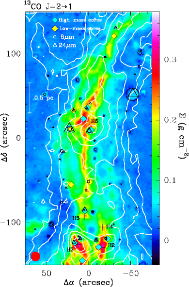
Figure 1: Integrated intensity image of the ¹³CO $J$=2$\rightarrow$1 line emission observed toward G035.39-00.33 with the IRAM 30m telescope for the velocity range from 40 to 50 km s^-1 (white contours). This image appears superimposed on the mass surface density map of the cloud (in colour; angular resolution of 2$"$; Kainulainen & Tan, 2013). For the ¹³CO $J$=2$\rightarrow$1 emission, the contour levels correspond to 33, 40, 50, 60, 70, 80 and 90% the peak integrated intensity of this image (40 K km s^-1). The linear intensity scale of the mass surface density map (in units of g cm^-2) is shown on the right side of the panel. Crosses indicate the location of the high-mass cores reported by Butler & Tan (2012). Black open circles and black open triangles show the 8 $\mu$m and 24 $\mu$m sources detected with Spitzer toward G035.39-00.33, respectively (Paper I, ). As in Paper I , the marker sizes have been scaled by the source flux. Yellow and light-blue filled diamonds show, respectively, the low-mass cores and the IR-quiet high-mass cores found by Nguyen Luong et al. (2011) with Herschel. The beam size of the ¹³CO $J$=2$\rightarrow$1 observations ($\sim$11$"$) is shown in the lower left corner of the panel.

In this paper, we report only the single-pointing spectra measured toward the most massive core in the mapped region, core H6 (Butler & Tan, 2012, and below), in an attempt to detect gas infall signatures in the line emission of HCO⁺ and HNC toward this core.

3 Results

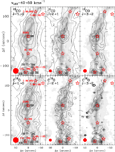
Figure 2: Integrated intensity images of the ¹³CO and C¹⁸O $J$=1$\rightarrow$0, $J$=2$\rightarrow$1 and $J$=3$\rightarrow$2 transitions for the velocity range from 40 to 50 km s^-1 (black contours), superimposed on the mass surface density map of Kainulainen & Tan (2013, in gray scale). The contour levels of the mass surface density map are 0.043, 0.074, 0.12, 0.16, 0.2, 0.25, and 0.29 g cm^-2, with the first contour corresponding to an extinction of $A_{v}$=10 mag. For the ¹³CO and C¹⁸O images, the contour levels are 35, 45, 60, 70, 80 and 90% the peak integrated intensity measured in every image, except for C¹⁸O $J$=3$\rightarrow$2 whose contour levels correspond to 45, 60, 70, 80 and 90% its measured peak integrated intensity. The peak integrated intensities for every image are 34.6 K km s^-1 for ¹³CO $J$=1$\rightarrow$0, 40.0 K km s^-1 for ¹³CO $J$=2$\rightarrow$1, 18.2 K km s^-1 for ¹³CO $J$=3$\rightarrow$2, 6.4 K km s^-1 for C¹⁸O $J$=1$\rightarrow$0, 9.0 K km s^-1 for C¹⁸O $J$=2$\rightarrow$1, and 3.3 K km s^-1 for C¹⁸O $J$=3$\rightarrow$2. Stars show the positions selected to extract the ¹³CO and C¹⁸O single-beam line spectra (Section 3.1 and Figure 3), and crosses indicate the location of the H cores reported by Butler & Tan (2012). The beam sizes of the IRAM 30m and JCMT observations are shown in the lower left corner of each panel.

In Figure 1, we present the integrated intensity map of the ¹³CO $J$=2$\rightarrow$1 line emission from $v_{\rm LSR}$=40 to 50 km s^-1 (white contours) observed with the IRAM 30m telescope toward the IRDC G035.39-00.33. This image has been superimposed on the mass surface density map of the cloud (in colour scale) derived by Kainulainen & Tan (2013) by combining a NIR extinction map with the MIR map of Butler & Tan (2012). In Figure 1, we also show the locations of the massive cores reported by Butler & Tan (2012) toward this cloud. The low-mass and the IR-quiet massive cores found by Nguyen Luong et al. (2011, see yellow and light-blue filled diamonds, respectively) from Herschel PACS and Spire data, are also shown. All these cores show emission at 70$\mu$m in the Herschel data. We note that the massive dense cores (filled light-blue diamonds) tend to cluster around the northern core H6 and the southern cores H2 and H3.

From Figure 1, we find that the observed ¹³CO $J$=2$\rightarrow$1 emission toward G035.39-00.33 mainly follows the filamentary structure of the IRDC seen in extinction. However, besides the main filament, two other molecular structures are detected toward the north-east and north-west of the cloud with faint counterparts seen in the mass surface density map.

The ¹³CO $J$=2$\rightarrow$1 main emission peaks are associated with the regions with highest extinction (i.e. densest) in the cloud at offsets (-4,10) and (10,-130). These are the regions where most of the IR-quiet massive cores are found (black crosses and light-blue diamonds; Rathborne et al., 2006; Butler & Tan, 2012; Nguyen Luong et al., 2011). While the ¹³CO $J$=2$\rightarrow$1 emission toward cores H3, H2 and H4 in the south of G035.39-00.33 traces the peaks of the mass surface density map, this emission is offset with respect to the densest peak in core H6. This is consistent with the significant CO depletion measured toward this core (depletion factor $f_{D}$$\sim$5 (Paper II, ; Paper III, ).

In Figure 2, we compare the morphology of the ¹³CO $J$=2$\rightarrow$1 emission with that from the ¹³CO $J$=1$\rightarrow$0 and $J$=3$\rightarrow$2 transitions, and from the C¹⁸O $J$=1$\rightarrow$0, $J$=2$\rightarrow$1 and $J$=3$\rightarrow$2 lines. The integrated intensity emission from 40 to 50 km s^-1 for all these lines is shown superimposed on the mass surface density map of Kainulainen & Tan (2013). Like for ¹³CO $J$=2$\rightarrow$1, the other ¹³CO and C¹⁸O transitions follow the filamentary structure seen in extinction. The ¹³CO $J$=1$\rightarrow$0 and $J$=2$\rightarrow$1 lines and the C¹⁸O $J$=1$\rightarrow$0 transition show the molecular extensions toward the north-east and north-west of G035.39-00.33. However, the higher-J ¹³CO $J$=3$\rightarrow$2 and C¹⁸O $J$=2$\rightarrow$1 and $J$=3$\rightarrow$2 lines probe denser (and therefore deeper) regions into the cloud as expected from their higher critical densities ($n_{\rm crit}$$\sim$3$\times$10⁴ cm^-2, i.e. a factor of $\geq$10 higher than those of the low-J lines, $n_{\rm crit}$$\sim$2$\times$10³ cm^-2). The high-J transitions of ¹³CO and C¹⁸O, therefore, suffer less from contamination from the diffuse molecular envelope of the IRDC.

3.1 Single-beam ¹³CO and C¹⁸O line spectra

Figure 3: Sample of ¹³CO and C¹⁸O $J$=1$\rightarrow$0, $J$=2$\rightarrow$1 and $J$=3$\rightarrow$2 line spectra observed toward six positions across G035.39-00.33 (see stars in Figure 2). The data have been smoothed to the 22$"$-beam of the IRAM 30m telescope at 110 GHz. Vertical dotted lines show the average of the central radial velocities measured in ¹³CO and C¹⁸O for every velocity component toward every position.

In Figure 3, we show a sample of the ¹³CO and C¹⁸O spectra observed at different positions across the IRDC. The spectra have been smoothed to the largest beam in the dataset (of 22$"$), corresponding to the $J$=1$\rightarrow$0 transition data. The positions are selected across the IRDC and are representative of cores H3 and H6 [offsets (10,-125) and (0,20)], of a position at half-distance between cores H2 and H4 [offset (-25,-115)], and of the more quiescent regions in the cloud [offsets (0,-50) and (-30,120)]. We have also selected a position off the main filament toward the northwest of the cloud [see offset (-60,110)].

From Figure 3, we find that the ¹³CO and C¹⁸O lines show complex molecular line profiles that change significantly across the IRDC. Consistent with the results from Paper IV , three different velocity components are detected from the ¹³CO and C¹⁸O emission. These velocity components are particularly clear toward (0,20), where the C¹⁸O lines show three emission peaks. In Table LABEL:tab3, we report the central radial velocities ($v_{\rm LSR}$), linewidths ($\Delta v$), and peak intensities (T_mb) of every velocity component derived by fitting the lines with three-component Gaussian profiles. The errors in $v_{\rm LSR}$ and $\Delta v$ are given by the uncertainties in the Gaussian fits, while the errors in T_mb correspond to the measured 1$\sigma$ rms level in the spectra. For the non-detections, the upper limits correspond to the 3$\sigma$ level in the ¹³CO and C¹⁸O spectra.

Table LABEL:tab3 shows that the observed velocity components are centered, approximately, at radial velocities $v_{\rm LSR}$$\sim$43, 45 and 46 km s^-1. However, a systematic trend is found for these velocities to become red-shifted (by $\sim$1.5 km s^-1) when one moves from the south to the north of G035.39-00.33 (note the systematic shift of the vertical dotted lines in Figure 3 from left to right). For instance, for the 43 km s^-1-component, the radial central velocity of ¹³CO $J$=1$\rightarrow$0 shifts from $v_{\rm LSR}$$\sim$42.9 km s^-1 toward (10,-125) in the south to $v_{\rm LSR}$$\sim$44.5 km s^-1 toward (-60,110) in the north. The same applies to the other two velocity components. As shown in Section 3.3, this velocity gradient in the CO isotopologue emission is confirmed by large-scale $v_{\rm LSR}$ maps across G035.39-00.33 (velocity gradient of $\sim$0.4-0.8 km s^-1 pc^-1; see Section 3.3).

The linewidths of the ¹³CO and C¹⁸O lines typically range from $\sim$1 to 2 km s^-1 (see Section 3.4 for the distribution of the ¹³CO and C¹⁸O linewidths), and the brightest ¹³CO and C¹⁸O emission arises from the velocity component at $\sim$45 km s^-1. This component, which contains the bulk of the molecular gas, is associated with the filamentary IRDC seen in extinction (Section 3.2). In the following, we describe in detail the morphology and kinematics of the different velocity components detected in ¹³CO and C¹⁸O toward G035.39-00.33.

Table 3: Observed parameters of the single-beam ¹³CO and C¹⁸O line spectra measured toward the selected positions shown in Figure 2.

	(10,-125)			(-25,-115)			(0,-50)
Transition	$v_{\rm LSR}$	$\Delta v$	Tmb	$v_{\rm LSR}$	$\Delta v$	Tmb	$v_{\rm LSR}$	$\Delta v$	Tmb
	(km s-1)	(km s-1)	(K)	(km s-1)	(km s-1)	(K)	(km s-1)	(km s-1)	(K)
13CO (1$\rightarrow$0)	42.93(0.11)	1.91(0.11)	5.9(0.5)	43.23(0.11)	2.31(0.11)	4.6(0.3)	42.49(0.05)	1.21(0.11)	1.4(0.2)
	44.65(0.11)	1.52(0.11)	6.4(0.5)	44.92(0.11)	1.19(0.11)	6.2(0.3)	44.87(0.14)	1.9(0.2)	6.3(0.2)
	45.88(0.11)	1.49(0.11)	5.8(0.5)	45.97(0.11)	1.10(0.11)	4.6(0.3)	46.21(0.10)	1.5(0.10)	5.2(0.2)
13CO (2$\rightarrow$1)	42.61(0.10)	1.69(0.12)	4.7(0.3)	43.17(0.11)	1.89(0.11)	4.2(0.3)	42.48(0.09)	1.2(0.2)	0.87(0.19)
	43.9(0.3)	1.93(0.11)	5.0(0.3)	44.58(0.11)	1.12(0.11)	5.3(0.3)	44.73(0.11)	1.85(0.17)	5.39(0.19)
	45.60(0.18)	2.3(0.2)	5.3(0.3)	45.81(0.11)	1.47(0.11)	4.5(0.3)	46.18(0.10)	1.57(0.11)	4.47(0.19)
13CO (3$\rightarrow$2)	42.83(0.11)	1.41(0.11)	2.03(0.16)	43.48(0.08)	1.82(0.14)	1.44(0.10)	$\ldots$	$\ldots$	$\leq$0.21
	44.31(0.11)	1.83(0.11)	2.77(0.16)	44.65(0.03)	0.86(0.07)	2.00(0.10)	45.02(0.10)	2.06(0.14)	2.09(0.07)
	45.86(0.11)	1.83(0.11)	1.93(0.16)	45.56(0.12)	1.6(0.2)	1.79(0.10)	46.27(0.05)	1.24(0.10)	1.22(0.07)
C18O (1$\rightarrow$0)	42.95(0.09)	1.87(0.19)	0.97(0.16)	42.98(0.10)	1.7(0.2)	0.65(0.15)	$\ldots$	$\ldots$	$\leq$0.36
	45.14(0.04)	1.59(0.11)	1.76(0.16)	45.07(0.03)	1.45(0.08)	1.84(0.15)	45.44(0.02)	1.91(0.04)	1.96(0.12)
	$\ldots$	$\ldots$	$\leq$0.48	$\ldots$	$\ldots$	$\leq$0.45	$\ldots$	$\ldots$	$\leq$0.36
C18O (2$\rightarrow$1)	42.98(0.11)	1.76(0.11)	1.54(0.08)	43.08(0.02)	1.08(0.07)	0.82(0.07)	$\ldots$	$\ldots$	$\leq$0.18
	45.24(0.11)	1.83(0.11)	1.73(0.08)	45.13(0.01)	1.53(0.03)	2.04(0.07)	45.54(0.09)	1.73(0.02)	1.97(0.06)
	$\ldots$	$\ldots$	$\leq$0.24	$\ldots$	$\ldots$	$\leq$0.21	$\ldots$	$\ldots$	$\leq$0.18
C18O (3$\rightarrow$2)	$\ldots$	$\ldots$	$\leq$0.36	$\ldots$	$\ldots$	$\leq$0.36	$\ldots$	$\ldots$	$\leq$0.27
	45.00(0.11)	2.2(0.2)	0.70(0.12)	45.06(0.04)	1.15(0.10)	0.83(0.12)	45.79(0.07)	1.99(0.16)	0.44(0.09)
	$\ldots$	$\ldots$	$\leq$0.36	$\ldots$	$\ldots$	$\leq$0.36	$\ldots$	$\ldots$	$\leq$0.27
	(0,20)			(-30,120)			(-60,110)
13CO (1$\rightarrow$0)	43.67(0.03)	2.05(0.05)	4.23(0.15)	44.36(0.11)	1.96(0.11)	3.6(0.5)	44.49(0.11)	1.20(0.11)	4.0(0.4)
	45.37(0.02)	1.378(0.019)	7.82(0.15)	46.00(0.11)	1.60(0.11)	6.8(0.5)	45.95(0.11)	1.04(0.11)	5.7(0.4)
	46.83(0.03)	1.683(0.05)	5.49(0.15)	47.11(0.11)	1.17(0.11)	3.4(0.5)	46.88(0.11)	1.25(0.11)	4.9(0.4)
13CO (2$\rightarrow$1)	43.32(0.11)	1.89(0.11)	2.49(0.15)	44.42(0.11)	2.15(0.11)	2.7(0.3)	44.72(0.07)	1.78(0.16)	2.6(0.2)
	45.25(0.11)	1.86(0.11)	6.88(0.15)	45.91(0.11)	1.52(0.11)	5.3(0.3)	46.01(0.03)	0.84(0.04)	4.2(0.2)
	46.90(0.11)	2.28(0.11)	3.57(0.15)	47.07(0.11)	1.18(0.11)	3.6(0.3)	46.88(0.02)	1.28(0.06)	3.7(0.2)
13CO (3$\rightarrow$2)	43.95(0.11)	2.20(0.11)	0.89(0.05)	44.4(0.13)	1.3(0.2)	0.64(0.11)	44.57(0.11)	0.48(0.11)	0.52(0.15)
	45.33(0.11)	1.68(0.11)	3.19(0.05)	46.05(0.03)	1.35(0.12)	3.02(0.11)	46.03(0.11)	0.94(0.11)	2.43(0.15)
	46.79(0.11)	2.05(0.11)	1.73(0.05)	47.19(0.04)	0.86(0.08)	1.39(0.11)	47.05(0.11)	1.41(0.11)	0.86(0.15)
C18O (1$\rightarrow$0)	43.59(0.04)	1.27(0.09)	0.95(0.10)	$\ldots$	$\ldots$	$\leq$0.55	$\ldots$	$\ldots$	$\leq$0.42
	45.29(0.02)	1.12(0.06)	2.14(0.10)	45.81(0.05)	1.14(0.14)	1.83(0.19)	46.19(0.05)	1.53(0.11)	1.00(0.14)
	46.74(0.03)	1.19(0.07)	1.45(0.10)	46.94(0.06)	0.66(0.12)	0.93(0.19)	$\ldots$	$\ldots$	$\leq$0.42
C18O (2$\rightarrow$1)	44.2(0.4)	2.7(0.5)	0.53(0.06)	44.9(0.3)	2.3(0.3)	0.41(0.07)	44.42(0.07)	0.86(0.11)	0.29(0.08)
	45.39(0.01)	1.07(0.05)	2.39(0.06)	45.82(0.02)	0.87(0.05)	1.38(0.07)	46.33(0.03)	1.74(0.07)	0.96(0.08)
	46.80(0.02)	1.22(0.04)	1.51(0.06)	46.73(0.02)	1.37(0.06)	0.91(0.07)	$\ldots$	$\ldots$	$\leq$0.24
C18O (3$\rightarrow$2)	44.06(0.11)	1.0(0.3)	0.19(0.06)	$\ldots$	$\ldots$	$\leq$0.24	$\ldots$	$\ldots$	$\leq$0.42
	45.28(0.03)	0.94(0.07)	1.01(0.06)	45.94(0.11)	0.96(0.11)	0.62(0.08)	$\ldots$	$\ldots$	$\leq$0.42
	46.68(0.06)	1.54(0.15)	0.57(0.06)	46.96(0.11)	0.90(0.11)	0.29(0.08)	$\ldots$	$\ldots$	$\leq$0.42

3.2 Channel maps of the ¹³CO and C¹⁸O emission

In Figures 4 and 5, we show the channel maps of the ¹³CO and C¹⁸O $J$=2$\rightarrow$1 line emission measured toward G035.39-00.33 between 41 and 49 km s^-1 in velocity increments of 0.5 km s^-1. We use the ¹³CO and C¹⁸O $J$=2$\rightarrow$1 line data cubes because they have the highest angular resolution available (beam of $\sim$11$"$) within our CO isotopologue molecular line dataset.

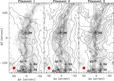
Figure 6: Integrated intensity images of the molecular Filaments 1, 2 and 3 seen in ¹³CO $J$=2$\rightarrow$1 toward G035.39-00.33. The velocity ranges of the maps are 42.5-44.5 km s^-1 for Filament 1, 44.5-46.0 km s^-1 for Filament 2, and 46.0-48.0 km s^-1 for Filament 3. The mass surface density map of Kainulainen & Tan (2013) is shown in gray scale (same as in Figure 2). The contour levels of the CO $J$=2$\rightarrow$1 emission are at 25, 35, 45, 60, 70, 80, and 90% the peak integrated intensity in every map (i.e. 20.5 K km s^-1, 12.6 K km s^-1, and 11.4 K km s^-1 for Filaments 1, 2 and 3 respectively). Crosses indicate the locations of the massive cores reported by Butler & Tan (2012). The beam size of the IRAM 30m observations ($\sim$11$"$) is shown in the lower left corner in every panel.

As noted in Paper IV , the general kinematics of the CO emission are characterized by the presence of several molecular filaments associated with the IRDC (Figure 4). The CO gas concentrates along, at least, two clear elongated/filamentary structures extending over $\sim$300$"$ (i.e. $\sim$4.4 pc) along the north-south direction. The first filament is seen at the velocity component at $v_{\rm LSR}$=43 km s^-1 (Filament 1). This filament runs from the north-east to the south-east, curving to the west towards the centre of the filament and showing a completely different morphology to that seen for the IRDC in extinction (the IRDC in extinction curves toward the east; see Figure 1). At more red-shifted velocities ($v_{\rm LSR}$$\sim$44.0-45.0 km s^-1), the CO molecular gas evolves from this filamentary morphology into a more complex structure. The dominant feature at these velocities has the same morphology as the IRDC seen in extinction and therefore it is associated with the densest part of the cloud (Filament 2; see Paper IV, ). Core H6 is approximately located at the intersecting region between Filaments 1 and 2 (Figure 4). For velocities $v_{\rm LSR}$$\geq$46 km s^-1 (Filament 3), the main filament develops two secondary extensions/arms toward the north-west and south-west of core H6. Although this new structure largely overlaps with Filament 2, it likely represents an additional feature different from Filaments 1 and 2 since it appears as an independent structure in velocity space with respect to the other two filaments (Paper IV, ). Figure 6 shows the integrated intensity images of the three individual molecular filaments (Filaments 1, 2 and 3) identified in G035.39-00.33 from the ¹³CO $J$=2$\rightarrow$1 emission.

From Figures 4 and 5, it is clear that the IR-quiet massive dense cores detected toward G035.39-00.33 tend to be found toward the regions where the filaments intersect, and where most of the molecular gas is concentrated. In particular, the chain of cores found toward the south follows the merged ¹³CO structure for Filaments 1 and 2 (see Figure 4 for the velocity range 44.5-45.0 km s^-1), suggesting that these structures are physically connected and likely interacting. The detection of broader ¹³CO and C¹⁸O line profiles toward these regions [offsets (10,-125) and (0,20) in Figure 3], could be due to the merging of the filaments, although on-going star-formation could also be responsible for the broadening of the lines. As reported in Paper I , broad SiO emission has been detected toward core H6 (SiO condensation named N) and toward core H4 (condensation S).

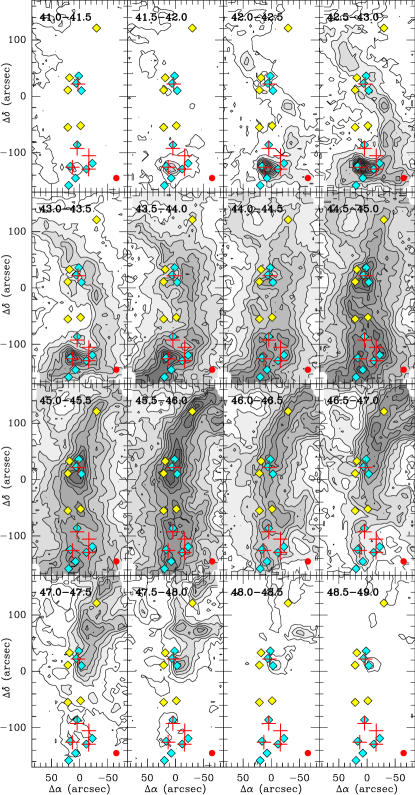
Figure 4: Channel maps of the ¹³CO $J$=2$\rightarrow$1 line emission toward G035.39-00.33 measured between 41 km s^-1 and 49 km s^-1 in velocity increments of 0.5 km s^-1. The velocity range of every map is shown at the upper left corner of every panel. The first contour and step levels are 0.50 (5$\sigma$) and 0.5 K km s^-1, respectively. Red crosses indicate the position of the dense cores reported by Butler & Tan (2012), and yellow filled diamonds and light-blue filled diamonds show the location of the low-mass and massive dense cores detected with Herschel (Nguyen Luong et al., 2011). The beam size of the ¹³CO $J$=2$\rightarrow$1 observations ($\sim$11^′′) is shown at the lower right corner in every panel.

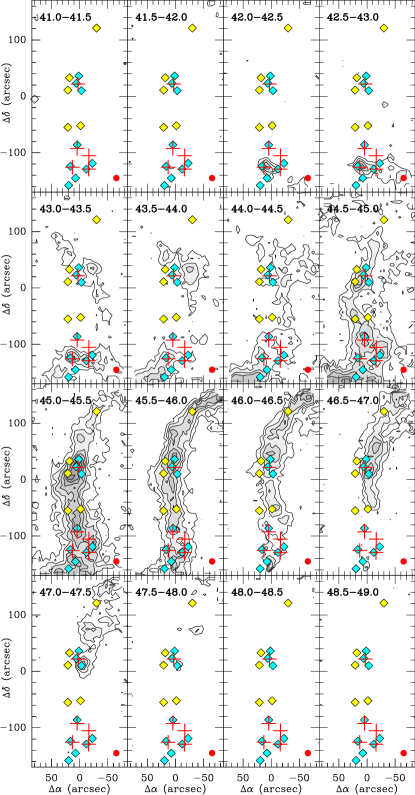
Figure 5: As in Figure 4 but for the C¹⁸O $J$=2$\rightarrow$1 line emission. The first contour and step levels are 0.40 (4$\sigma$) and 0.3 K km s^-1, respectively. Crosses and symbols are as in Figure 4.

3.3 Distribution of v_LSR across the CO filaments

By using the single-dish spectra of ¹³CO and C¹⁸O measured across G035.39-00.33, we can derive the distribution of the central radial velocity, $v_{\rm LSR}$, and linewidth, $\Delta v$, of the molecular gas for every position in this IRDC. We use the $J$=2$\rightarrow$1 and $J$=3$\rightarrow$2 transitions of ¹³CO and C¹⁸O because they probe denser gas than the $J$=1$\rightarrow$0 lines, and their maps have a higher angular resolution (beam of $\sim$11$"$-14$"$; Table LABEL:tab1). In this Section, we will report the results from the $v_{\rm LSR}$ maps, while the distribution of $\Delta v$ for the ¹³CO and C¹⁸O lines will be presented in Section 3.4.

To calculate the $v_{\rm LSR}$ and $\Delta v$ maps across G035.39-00.33, we have smoothed the ¹³CO and C¹⁸O single-dish $J$=2$\rightarrow$1 and $J$=3$\rightarrow$2 data to the same angular resolution of 14$"$ (i.e. to the largest beam of the JCMT maps), so that the $J$=2$\rightarrow$1 and $J$=3$\rightarrow$2 spectra can be compared directly. The individual spectra are simultaneously fitted with three-component Gaussian line profiles as described in Appendix A. In our analysis of the ¹³CO lines, we have considered line spectra with peak intensities $\geq$9$\sigma$ only (with $\sigma$ the rms in every spectrum). This criterion was first used in Paper IV and takes into account that the typical detection threshold for Gaussian line profiles is 3$\sigma$ and that the ¹³CO emission toward G035.39-00.33 has three overlapping velocity components. For C¹⁸O, the applied detection threshold is $\geq$5$\sigma$ since the C¹⁸O lines are weaker (Appendix A). The derived values of $v_{\rm LSR}$ and $\Delta v$ are then used to generate the $v_{\rm LSR}$ and $\Delta v$ maps. This Gaussian decomposition allows to study not only the individual kinematic structure of every filament, but also the excitation conditions of the CO gas within them (see Section 4).

In Figure 7, we show the distribution of $v_{\rm LSR}$ derived from the ¹³CO $J$=2$\rightarrow$1 data for Filaments 1, 2 and 3. The intensity-weighted average of $v_{\rm LSR}$ for every filament is shown in the upper part of every panel, and is calculated as described in Appendix B. The intensity-weighted average of $v_{\rm LSR}$ is 43.61 km s^-1 for Filament 1, 45.16 km s^-1 for Filament 2, and 46.47 km s^-1 for Filament 3 (Table LABEL:tab4). In agreement with the results reported in Paper IV , the filaments are separated in velocity space by $\sim$3 km s^-1. We note that these values change by $<$0.2% if data with peak intensities $\geq$5$\sigma$, instead of $\geq$9$\sigma$, are considered in our analysis.

For all three filaments, our data reveal a velocity gradient in the north-south direction with the red-shifted gas peaking toward the north-northwest of G035.39-00.33, and with the blue-shifted emission toward the south of this cloud. While the most red- and blue-shifted velocities are measured at distances further away from core H6, the ¹³CO gas motions in the vicinity of this core show radial velocities close to the average values (i.e. the gas radial velocities get more red- or blue-shifted with increasing distance to core H6; see Figure 7). Although the velocity gradient is relatively smooth for Filament 2, we note that the kinematics of the ¹³CO gas in the vicinity of this core for Filaments 1 and 3 are more complex. This could be due either to feedback from local star formation (broad SiO emission is detected toward this position; see Paper I, ) or to smaller-scale structures unresolved in our single-dish observations (see Section 5.4 and Henshaw et al. 2013b).

The derived values for the velocity gradient are $\sim$0.4-0.8 km s^-1 pc^-1 from the northern part of G035.39-00.33 to core H6, and $\sim$0.6-0.8 km s^-1 pc^-1 from the southern region to this core. This velocity gradient is consistent with that previously reported in Paper IV (of $\sim$1 km s^-1 pc^-1) for Filament 2. Similar velocity gradients have also been reported toward the Orion molecular cloud ($\sim$0.7 km s^-1 pc^-1; Bally et al., 1987), the DR21 filament ($\sim$0.8-2.3 km s^-1 pc^-1; Schneider et al., 2010), or even toward the low-mass Serpens South cluster-forming region ($\sim$1.4 km s^-1 pc^-1; Kirk et al., 2013). This smooth velocity gradient in G035.39-00.33 has become apparent thanks to the new ¹³CO and C¹⁸O data, and contrasts with the sharp velocity transition found in Paper IV . This is likely due to the lower-angular resolution of the N₂H⁺ and C¹⁸O $J$=1$\rightarrow$0 data compared to our ¹³CO $J$=2$\rightarrow$1 line data ($\sim$26$"$ vs. 14$"$, respectively). We also stress that the smooth velocity gradient reported for every filament cannot be attributed to an artifact of our three-component Gaussian fit method, since the close inspection of the single-pointing spectra (Section 3.1) already revealed a systematic trend for the radial velocities of the filaments to shift from blue- to red-shifted velocities as one moves from the southern to the northern regions in the IRDC.

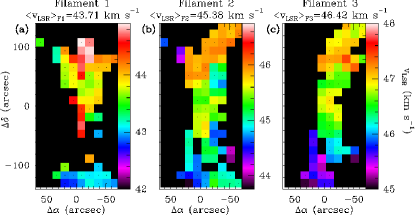
Figure 14: As in Figure 7, but obtained from the C¹⁸O $J$=2$\rightarrow$1 line data. We have only plotted the positions where the derived peak intensity of the C¹⁸O $J$=2$\rightarrow$1 emission is brighter than 5$\sigma$, with $\sigma$ the rms level in each spectrum.

Besides ¹³CO $J$=2$\rightarrow$1, the analysis of the ¹³CO $J$=3$\rightarrow$2 and C¹⁸O $J$=2$\rightarrow$1 data also reveals a similar behavior for the individual motions of the gas within every filament (see Figures 13 and 14). This demonstrates that our analysis of the kinematics of the molecular gas toward G035.39-00.33 does not depend on the transition used, and provides robust results against the multi-Gaussian profile fitting method described in Appendix A. Indeed, the average $v_{\rm LSR}$ derived for every filament is very similar in all transitions and CO isotopologues (see Table LABEL:tab4), except for Filament 2 where the C¹⁸O $J$=2$\rightarrow$1 emission appears globally red-shifted (by $\sim$0.2 km s^-1) compared to the lower-density ¹³CO $J$=2$\rightarrow$1 line. This behavior is similar to that reported between C¹⁸O $J$=1$\rightarrow$0 and N₂H⁺ $J$=1$\rightarrow$0, and has been interpreted as a signature of the ongoing interaction between Filaments 1 and 2 (Paper IV, ). This velocity shift cannot be attributed to large optical depth effects since ¹³CO and C¹⁸O are moderately optically thick and optically thin, respectively (see Sections 4.1 and 4.2).

The emission from the C¹⁸O $J$=3$\rightarrow$2 is very faint throughout the map except for few positions (see Figure 2). This has prevented us from generating the individual motions of the three filaments from this transition.

3.4 Distribution of $\Delta v$ in the CO filaments

Table 4: Intensity-weighted average of $v_{\rm LSR}$, $\Delta v$, and $\sigma_{\rm NT}$ for Filaments 1, 2 and 3.

	$<v_{\rm LSR}>$			$<\Delta v>_{\rm F_{k}}$			$\sigma_{\rm NT}$
	(km s-1)			(km s-1)			(km s-1)
Transition	F1	F2	F3	F1	F2	F3	F1	F2	F3
13CO (2$\rightarrow$1)	43.61	45.16	46.47	1.78	1.75	1.59	0.71	0.70	0.62
13CO (3$\rightarrow$2)	43.72	45.24	46.54	1.47	1.48	1.40	0.57	0.57	0.54
C18O (2$\rightarrow$1)	43.71	45.38	46.42	1.30	1.21	1.15	0.49	0.44	0.42

Note.- $<v_{\rm LSR}>$, $<\Delta v>$, and $\sigma_{\rm NT}$ are calculated for positions where the peak intensities are $\geq$9$\sigma$ for ¹³CO $J$=2$\rightarrow$1 and $J$=3$\rightarrow$2, and $\geq$5$\sigma$ for C¹⁸O $J$=2$\rightarrow$1.

We have generated maps of the average linewidth of the ¹³CO and C¹⁸O lines, $<\Delta v>_{\rm Tot}$, by using the linewidths measured for every velocity component (or filament) and position in the map (see Appendix B for the method to calculate this average). By doing this, we can infer the global level of turbulence across the cloud, and look for any systematic changes in the molecular linewidths between the densest regions in the IRDC and its lower-density envelope.

In Figure 8, we report the maps of $<\Delta v>_{\rm Tot}$ derived for ¹³CO $J$=2$\rightarrow$1, ¹³CO $J$=3$\rightarrow$2, and C¹⁸O $J$=2$\rightarrow$1 toward G035.39-00.33. From Figure 8, we find that the general distribution of $<\Delta v>_{\rm Tot}$ for ¹³CO $J$=2$\rightarrow$1 is not uniform and shows broader line emission along the outer edges of the IRDC. This behaviour was already noted in Paper II, and resembles that reported by Pineda et al. (2010) toward the B5 low-mass star forming core. Since we only consider the positions in the ¹³CO $J$=2$\rightarrow$1 map with line detections $\geq$9$\sigma$, the line broadening toward the outer regions in G035.39-00.33 is not due to poorer quality of the Gaussian fits, but to a real increase in the velocity dispersion in the lower density gas. The spatial distribution of $<\Delta v>_{\rm Tot}$ for ¹³CO $J$=3$\rightarrow$2 and C¹⁸O $J$=2$\rightarrow$1 shows narrower linewidths toward the central regions of G035.39-00.33, supporting this idea. Indeed, the average linewidths $<\Delta v>_{\rm F_{k}}$ of the individual filaments in G035.39-00.33 (see Appendix B and Table LABEL:tab4) are significantly narrower for ¹³CO $J$=3$\rightarrow$2 and C¹⁸O $J$=2$\rightarrow$1 (i.e. $\sim$1.4-1.5 and 1.2-1.3 km s^-1, respectively) than for ¹³CO $J$=2$\rightarrow$1 ($\sim$1.6-1.8 km s^-1), which could be related to energy dissipation. The derived values of $<\Delta v>_{\rm F_{k}}$ are found to vary by $<$3% if data with peak intensities $\geq$5$\sigma$, instead of $\geq$9$\sigma$, are considered in our analysis.

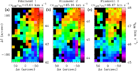
Figure 7: Spatial distribution of $v_{\rm LSR}$ derived from ¹³CO $J$=2$\rightarrow$1 for Filaments 1, 2 and 3 (panels (a), (b), and (c), respectively). Only data with intensities $\geq$9$\sigma$ are plotted. Color scale is shown on the right of every panel. Note that the velocity range varies from panel to panel. The intensity-weighted average of the radial velocity for every filament, $<v_{\rm LSR}>_{\rm F_{k}}$, is shown at the upper part of panels (a), (b), and (c) (Table LABEL:tab4). The kinematics of the molecular gas reveal a smooth north-south velocity gradient along the IRDC, consistent with gas accretion onto core H6 along the filaments (see Section 3.3).

The trend of increasing linewidth toward the low-density outer regions of the IRDC can also be seen from the distribution of the non-thermal (turbulent) velocity dispersion, $\sigma_{\rm NT}$, for the individual Filaments 1, 2 and 3. $\sigma_{\rm NT}$ can be determined from the observed linewidth, $\Delta v$, as follows (Myers, 1983):

$$\sigma_{\rm NT}=\sqrt{\frac{\Delta v^{2}}{8\,\,ln2}-\frac{k_{B}\,\,T_{\rm kin}}{m}},$$ (1)

where $k_{B}$ is the Boltzmann’s constant, $T_{\rm kin}$ the kinetic temperature of the molecular gas, and $m$ the mass of the molecular species (either 29 a.m.u. for ¹³CO or 30 a.m.u. for C¹⁸O). The thermal dispersion of the molecular gas, $\sigma_{T}$=$\sqrt{k_{B}T_{\rm kin}/m}$, is $\sim$0.07 km s^-1 assuming that the gas kinetic temperature is 15 K (Pillai et al., 2006; Ragan et al., 2011; Fontani et al., 2012). Table LABEL:tab4 reports the values of $\sigma_{\rm NT}$ derived for every filament.

In Figure 9, we show the non-thermal velocity dispersion, $\sigma_{\rm NT}$, derived from the ¹³CO and C¹⁸O data as a function of peak intensity, T_mb, for every filament. To our knowledge, this is the first attempt made to measure the non-thermal velocity dispersion across different filaments within the same IRDC. The peak intensity, T_mb, of these lines is used as a proxy of column density and, therefore, of the radial distance to the axis of the filaments. In order to better show the increasing trend of $\sigma_{\rm NT}$ for decreasing T_mb, we have carried out a power law fit to the data in the form $\sigma_{\rm NT}$=$a\times(T_{\rm mb})^{b}$ (see red lines in Figure 9). For the fits, we have binned the data in temperature ranges of 0.25 K. While the average $b$ parameter for ¹³CO $J$=2$\rightarrow$1 is $\sim$$-$0.24, for ¹³CO $J$=3$\rightarrow$2 this parameter is $b$$\sim$$-$0.09, indicating a weaker dependency of $\sigma_{\rm NT}$ with radial distance. As expected for a higher-density tracer, C¹⁸O $J$=2$\rightarrow$1 shows almost a flat distribution with an average $b$ value $\sim$$-$0.03.

From Figure 9, we find that the gas in the individual molecular filaments of G035.39-00.33 is supersonic, with an average non-thermal velocity dispersion $\sigma_{\rm NT}$ (see also Table LABEL:tab4) being factors $\sim$2-3 larger than the sound speed in the medium (i.e. sound Mach number $\sim$2-3 with the sound speed being $c_{s}$=0.25 km s^-1). This is in agreement with the results by Vasyunina et al. (2011) and Ragan et al. (2012) toward two samples of IRDCs, and contrasts with the gas motions toward the molecular filaments in the L1517 and the L1495/B213 low-mass star forming regions, where these motions are, respectively, subsonic and mildly transonic toward both the high-density cores (seen in N₂H⁺) and the lower-density envelope of the filaments probed by C¹⁸O (see Hacar & Tafalla, 2011; Hacar et al., 2013).

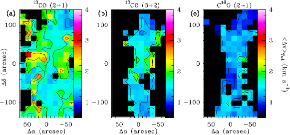
Figure 8: Maps of the intensity-weighted average of the linewidth (in km s^-1) obtained across the IRDC G035.39-00.33, $<\Delta v>_{\rm Tot}$ (in colour) for the ¹³CO $J$=2$\rightarrow$1 (panel (a)), ¹³CO $J$=3$\rightarrow$2 (panel (b)), and C¹⁸O $J$=2$\rightarrow$1 lines (panel (c)). Colour scale is shown on the right in every panel. Contours are 1.25, 1.75, and 2.25 km s^-1 for ¹³CO $J$=2$\rightarrow$1 and ¹³CO $J$=3$\rightarrow$2, with the narrower linewidths found toward the central regions of the IRDC. For C¹⁸O $J$=2$\rightarrow$1, contours are 1.0, 1.5, and 2.0 km s^-1, showing a flatter linewidth distribution.

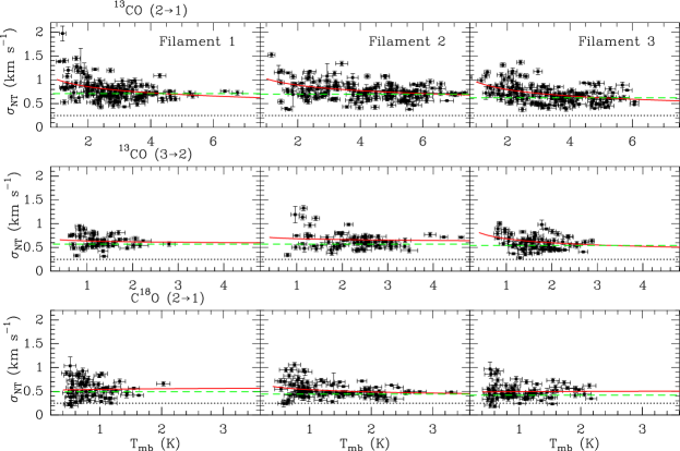
Figure 9: Non-thermal velocity dispersion derived from ¹³CO $J$=2$\rightarrow$1 and $J$=3$\rightarrow$2, and from C¹⁸O $J$=2$\rightarrow$1, toward every position in Filaments 1, 2 and 3, and represented as a function of peak intensity (in units of T_mb). For ¹³CO $J$=2$\rightarrow$1 and $J$=3$\rightarrow$2, we only consider data points with T_mb$\geq$9$\sigma$, while for C¹⁸O $J$=2$\rightarrow$1, we impose that T_mb$\geq$5$\sigma$. Horizontal dotted lines show the value of the sound speed of the average particle ($\mu$=2.33) at T_kin=15 K ($c_{s}$=0.25 km s^-1). Green dashed lines show the average non-thermal dispersion of every filament and transition (Table LABEL:tab4). Red lines show the power law fit to the data in the form $\sigma_{\rm NT}$=$a\times(T_{\rm mb})^{b}$ (see text for a and b values).

3.5 Gas infall tracer lines toward core H6

In Section 3.3, we have reported the detection of a relatively smooth velocity gradient of $\sim$0.4-0.8 km s^-1 pc^-1 in the north-south direction, common to Filaments 1, 2 and 3. As discussed in Section 5.2, one scenario that could explain this velocity gradient is gas accretion flows along Filaments 1, 2 and 3 onto the massive core H6. We investigate whether typical gas infall tracers such as HCO⁺ and HNC indeed show blue-shifted asymmetries in their self-absorbed molecular line profiles as a result of gas accretion onto this core.

In Figure 10 we report the spectra of the $J$=1$\rightarrow$0 lines of HCO⁺, HNC, H¹³CO⁺ and HN¹³C, and of the $J$=3$\rightarrow$2 transition of HCO⁺, measured toward core H6, and smoothed to the same angular resolution of 29$"$ (the largest beam of the IRAM 30m observations). All species show similar line profiles. In particular, the emission from optically thick tracers, HCO⁺ and HNC, peaks at the same $v_{\rm LSR}$ ($\sim$45.4 km s^-1, i.e. the $v_{\rm LSR}$ derived for the dense C¹⁸O $J$=2$\rightarrow$1 gas; see Table LABEL:tab4) as their optically thin ¹³C isotopologues, H¹³CO⁺ and HN¹³C. This clearly contrasts with the behaviour seen for self-absorbed spectra toward contracting cloud cores, for which the optically thin species show their emission peaks red-shifted compared to the optically thick lines (see Myers, 1995; Kirk et al., 2013; Peretto et al., 2013). The asymmetry in the line profiles of HCO⁺ and HNC found toward core H6 are probably not due to gas infalling onto this core (at least at angular scales of $\geq$29$"$, or $\geq$0.4 pc), but to the intrinsic kinematic structure of the IRDC (Section 3.2). We note that infall motions are not likely to appear at the denser regions in this IRDC since the HCO⁺ $J$=3$\rightarrow$2 emission does not show any self-absorption toward core H6 either.

4 Excitation conditions of the CO gas in G035.39-00.33

We can now use the derived peak intensities and linewidths of the ¹³CO and C¹⁸O $J$=2$\rightarrow$1 and $J$=3$\rightarrow$2 lines, to estimate the physical conditions of the gas such as H₂ number density, n(H₂), ¹³CO/C¹⁸O column density, N(¹³CO) or N(C¹⁸O), excitation temperature, T_ex, and optical depth, $\tau$, in the three molecular filaments detected toward G035.39-00.33 (Sections 3.1 and 3.2). To do this, we have used the Large Velocity Gradient (LVG) approximation (Sobolev, 1947), for which we have considered the collisional coefficients of ¹³CO and C¹⁸O with H₂ calculated by Yang et al. (2010), and the first 18 rotational levels of these two molecules. We assume a kinetic temperature of the gas, T_kin, of $\sim$15 K, which is similar to those found in other IRDCs from NH₃ observations (Pillai et al., 2006; Ragan et al., 2011; Fontani et al., 2012), and which is in close equilibrium with the temperature of the dust measured toward G035.39-00.33 (T_d$\sim$16-17 K; see Nguyen Luong et al., 2011). In Section 4.3, we however evaluate the sensitivity of our LVG results to small changes in the kinetic temperature.

The average linewidth between the $J$=2$\rightarrow$1 and $J$=3$\rightarrow$2 lines of ¹³CO and C¹⁸O was used as an input parameter in the LVG code. The $J$=1$\rightarrow$0 line emission from ¹³CO and C¹⁸O was not employed in our calculations because 1) this transition probes lower-density gas in the IRDC (Paper II, ); and 2) all data would have to be smoothed to the poorer angular resolution of $\sim$22$"$ of the $J$=1$\rightarrow$0 observations (Table LABEL:tab1). In Section 4.4, we examine in what extent our LVG results are modified by the inclusion of the $J$=1$\rightarrow$0 data in the LVG analysis.

A grid of LVG models were run with H₂ number densities ranging from 900 cm^-3 to $\sim$10⁵ cm^-3, and with ¹³CO and C¹⁸O column densities ranging from 10¹⁰ cm^-2 to $\sim$10²⁰ cm^-2. For every grid position, the LVG code calculates the peak intensity of the rotational lines of a molecular species (i.e. ¹³CO or C¹⁸O in our case) with quantum numbers from $J_{\rm up}$=1 to $J_{\rm up}$=18. The LVG solution is then obtained by means of a minimization technique by comparing the predicted intensities of the $J$=2$\rightarrow$1 line and the predicted line intensity ratio T(3$\rightarrow$2)/T(2$\rightarrow$1), with those observed toward every position in the map. For ¹³CO, only those positions across the IRDC where both transitions were detected above the 9$\sigma$ level, were considered in the calculations (i.e. we use the same dataset as that reported in Sections 3.3 and 3.4). Note that this is important because it guarantees that the derived peak intensities and linewidths of the lines, key for the determination of the physical conditions of the gas, have been measured with good accuracy. The LVG results provide maps of n(H₂), N(¹³CO), T_ex and $\tau$ (see Section 4.1). However, in the case of C¹⁸O, the threshold of 5$\sigma$ for both transitions was exceeded only toward three positions across the IRDC (see Section 4.2), including 1) core H6; 2) the C¹⁸O emission peak toward the west of core H6; and 3) 10$"$ north the position where narrow SiO emission lines have been detected (Paper I, ).

4.1 LVG results for ¹³CO

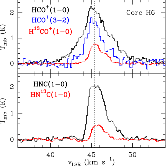
Figure 10: Spectra of the HCO⁺ $J$=1$\rightarrow$0, HCO⁺ $J$=3$\rightarrow$2, H¹³CO⁺ $J$=1$\rightarrow$0, HNC $J$=1$\rightarrow$0, and HN¹³C $J$=1$\rightarrow$0 lines measured toward core H6. The spectra have been smoothed to the largest beam of $\sim$29$"$ of the IRAM 30m data. The vertical dotted line indicates the $v_{\rm LSR}$ of the dense C¹⁸O $J$=2$\rightarrow$1 gas in Filament 2 ($v_{\rm LSR}$$\sim$45.4 km s^-1; see Table LABEL:tab4).

Table 5: Average physical properties of Filaments 1, 2 and 3 derived from ¹³CO for T_kin=13 K, 15 K and 17 K.

Filament	Tkin	n(H2)	N(13CO)	Tex(2$\rightarrow$1)	Tex(3$\rightarrow$2)	$\tau_{\rm 21}$	$\tau_{\rm 32}$	$\Sigma_{\rm{}^{13}CO}$	Mass
	(K)	(cm-3)	(cm-2)	(K)	(K)			(g cm-2)	(M⊙)
1	13	8000	1.1$\times$1016	9.7	7.9	2.2	1.4	0.014	5700
2	13	8600	2.4$\times$1016	10.4	8.5	4.5	3.3	0.030	27000
3	13	11500	1.2$\times$1016	10.2	8.4	2.7	1.8	0.015	13300
1	15	5100	9.4$\times$1015	9.7	7.8	2.0	1.3	0.012	4300
2	15	7500	1.4$\times$1016	11.0	8.9	2.7	2.0	0.020	15000
3	15	7300	9.6$\times$1015	10.7	8.6	2.2	1.5	0.012	10800
1	17	4000	8.2$\times$1015	9.9	7.9	1.8	1.1	0.010	3800
2	17	5600	1.3$\times$1016	11.3	9.0	2.5	2.0	0.016	14500
3	17	5500	8.9$\times$1015	10.9	8.7	2.0	1.4	0.011	9900

In Figure 11, we present the H₂ number density, n(H₂), ¹³CO column density, N(¹³CO), and excitation temperature of the gas for the $J$=2$\rightarrow$1 transition, T_ex(2$\rightarrow$1), obtained for Filament 1 (upper panels), Filament 2 (middle panels), and Filament 3 (lower panels) by using the LVG approximation. Table LABEL:tab5 also reports the average values of these parameters measured for every filament. From Figure 11, we find that the derived n(H₂) typically range between some 10³ cm^-3 to few 10⁴ cm^-3, as expected for a low-density tracer such as ¹³CO, and in agreement with those H₂ densities estimated toward low-mass molecular clouds such as Perseus (see e.g. Bensch, 2006; Pineda et al., 2008). The average H₂ density for Filament 1 is somewhat smaller ($\sim$5100 cm^-3) than those of Filaments 2 and 3 ($\sim$7300-7500 cm^-3; see Table LABEL:tab5), indicating that the former filament is less dense than the latter ones. This was already noted in Paper IV from the lack of N₂H⁺ $J$=1$\rightarrow$0 emission in Filament 1.

The derived ¹³CO column densities range from $\sim$2-3$\times$10¹⁵ cm^-2 to $\sim$2-3$\times$10¹⁶ cm^-2 in the three filaments. The average values of N(¹³CO) are very similar in the three filaments and are $\sim$10¹⁶ cm^-2 (Table LABEL:tab5). Assuming an isotopic ratio ¹²C/¹³C of 53 (Wilson & Rood, 1994), a CO abundance of $\chi$(CO)$\sim$2$\times$10^-4 (Lacy et al., 1994), and a mass per H nucleus of $\mu_{H}$=2.34$\times$10^-24 g, we can derive the average mass surface density for every filament as:

$$\Sigma_{\rm 13CO}=1.24\times 10^{-2}\times\left[\frac{N(\rm^{13}CO)}{10^{16}(\rm cm^{-2})}\right]\,\,\rm g\,\,\,cm^{-2}.$$ (2)

The average values of N(¹³CO) imply mass surface densities of $\sim$0.012 g cm^-2 for Filaments 1 and 3, and of $\sim$0.02 g cm^-2 for Filament 2 (Table LABEL:tab5). By adding up all these contributions, we obtain a total surface mass density $\sim$0.04 g cm^-2, which is consistent with the average value obtained in Paper II from their C¹⁸O data.

An estimate of the relative H₂ gas masses between the filaments can be derived from the values of N(¹³CO) shown in Figure 11. As shown in Table LABEL:tab5, the derived H₂ gas masses for Filaments 1, 2 and 3 are, respectively, 4300, 15000 and 10800 M_⊙. This implies that Filament 1 is a factor of $\sim$2-3 less massive than Filaments 2 and 3, while the latter two filaments have very similar gas masses. One may think that the lower mass for Filament 1 could be a consequence of the smaller number of data points considered in the calculation. However, by using a similar area than that covered by Filaments 2 and 3, and by assuming an average column density of N(¹³CO)=2$\times$10¹⁵ cm^-2, the estimated gas mass missing for Filament 1 is $\sim$300 M_⊙ (i.e. $\sim$7% its total gas mass). After including this gas mass correction, Filament 1 is still 2-3 times less massive than Filaments 2 and 3.

From Figure 11, we also find that the excitation temperature for the $J$=2$\rightarrow$1 transition, T_ex(2$\rightarrow$1), ranges from $\sim$7 K to $\sim$14 K in the three filaments. The average values of T_ex(2$\rightarrow$1) are 10-11 K (Table LABEL:tab5), showing that the ¹³CO gas is sub-thermally excited. These excitation temperatures are similar to those found toward low-mass dark clouds (Pineda et al., 2008). We note however that T_ex(2$\rightarrow$1) tends to increase to $\sim$13-14 K toward the eastern edge of the IRDC for Filaments 2 and 3, as a consequence of the higher H₂ densities found in these regions (Figure 11). This behaviour is similar to that found in Paper IV from N₂H⁺ data. The measured values of T_ex(3$\rightarrow$2) are typically $\sim$2 K below those reported for T_ex(2$\rightarrow$1).

The average optical depth obtained from our LVG results for the ¹³CO $J$=2$\rightarrow$1 and $J$=3$\rightarrow$2 lines is, respectively, $\tau_{\rm 21}$$\sim$2-3 and $\tau_{\rm 32}$$\sim$1-2 (see Table LABEL:tab5). This indicates that the ¹³CO emission is moderately optically thick.

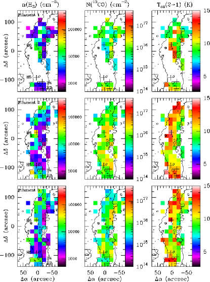
Figure 11: H₂ number density, n(H₂), ¹³CO column density, N(¹³CO), and excitation temperature, T_ex, derived from ¹³CO $J$=2$\rightarrow$1 and $J$=3$\rightarrow$2 for Filament 1 (upper panels), Filament 2 (middle panels) and Filament 3 (lower panels) using the LVG approximation. Overlapped onto these maps, we also show the mass surface density map derived by Kainulainen & Tan (2013) in silhouette. Colour scale is shown on the right side of every panel. Crosses indicate the location of the cores reported by Butler & Tan (2012).

4.2 LVG results for C¹⁸O

The C¹⁸O data toward G035.39-00.33 reveal only three positions in Filaments 2 and 3 where the $J$=2$\rightarrow$1 and $J$=3$\rightarrow$2 lines are both brighter than the 5$\sigma$ level in the C¹⁸O spectra. These positions are: 1) core H6; 2) a C¹⁸O emission peak toward the west of core H6 (the C¹⁸O West Peak at offset (-9,24); Figure 2); and 3) offset (-9,80) located 10$"$ north the region where narrow SiO has been detected (the Narrow SiO Peak; see Paper I, ). In Table LABEL:tab6, we report the H₂ density, C¹⁸O column density, and excitation temperature and optical depth for the $J$=2$\rightarrow$1 and $J$=3$\rightarrow$2 transitions, obtained with the LVG approximation and by using the C¹⁸O $J$=2$\rightarrow$1 and $J$=3$\rightarrow$2 spectra smoothed within a 14$"$-beam toward each position. From this Table, we find that core H6 is the densest of the three regions with a H₂ number density of $\sim$10⁴ cm^-3. The H₂ densities for the C¹⁸O West peak and the Narrow SiO Peak are of $\sim$2-4$\times$10³ cm^-3. The C¹⁸O column densities are however very similar toward the three positions, with values within a factor of 1.5. The derived excitation temperatures are similar to those measured for ¹³CO, and the optical depths are $\leq$1, indicating that the emission from the C¹⁸O lines is optically thin. This is consistent with the results of Paper II .

From C¹⁸O $J$=1$\rightarrow$0 and $J$=2$\rightarrow$1 observations, in Paper II we found that G035.39-00.33 shows widespread CO depletion with depletion factors, $f_{D}$, as high as $\sim$5. Since the $J$=3$\rightarrow$2 line emission has a higher critical density ($n_{\rm crit}$$\sim$5$\times$10⁴ cm^-3) than the $J$=1$\rightarrow$0 and $J$=2$\rightarrow$1 lines ($n_{\rm crit}$$\sim$2$\times$10³ cm^-3 and $\sim$8$\times$10³ cm^-3, respectively), our LVG results obtained using the C¹⁸O $J$=3$\rightarrow$2 data have the potential to provide the depletion factor toward even denser regions with a higher degree of CO depletion. Following the notation used in Paper II , we can calculate the depletion factor, $f_{D}$, as:

$$f_{D}=\frac{\Sigma_{\rm SMF}}{\Sigma_{\rm C18O}},$$ (3)

where $\Sigma_{\rm SMF}$ denotes the mass surface density derived from near- and mid-IR images (Kainulainen & Tan, 2013), and $\Sigma_{\rm C18O}$ is the mass surface density obtained from the observed C¹⁸O column density toward Filaments 2 and 3. To calculate $\Sigma_{\rm C18O}$, we have used Eq. 5 from Paper II , and assumed an ¹⁶O/¹⁸O isotopic ratio of 327 (Wilson & Rood, 1994), and a CO fractional abundance of 2$\times$10^-4 (Lacy et al., 1994).

In Table LABEL:tab6, we report the $\Sigma_{\rm SMF}$, the $\Sigma_{\rm C18O}$ and the CO depletion factor measured toward core H6, the C¹⁸O West Peak, and the Narrow SiO Peak. The derived CO depletion factor is $f_{D}$$\sim$5-12. In particular, toward core H6, this value is a factor of $\geq$2 higher than those reported in Paper II . The CO depletion factors measured toward G035.39-00.33 are thus similar to those derived toward low-mass pre-stellar cores (e.g. Crapsi et al., 2005), and consistent with those recently estimated toward a sample of IRDCs (Fontani et al., 2012). This is expected to largely affect the deuterium chemistry, as found toward massive starless cores where the deuterium fractionation, D_frac, is increased by a factor of 10 with respect to more evolved high-mass protostellar objects (see Fontani et al., 2011).

4.3 Sensitivity of the LVG results to T_kin

In Sections 4.1 and 4.2, we have assumed that the kinetic temperature of the gas in G035.39-00.33 is T_kin=15 K. However, as measured from NH₃ observations toward other IRDCs (see e.g. Pillai et al., 2006; Ragan et al., 2011), T_kin could range from $\sim$11 K to 18 K. We evaluate the effects of T_kin on our LVG study by considering a kinetic temperature of $\pm$2 K with respect to T_kin=15 K. In Table LABEL:tab5, we compare the LVG results obtained for T_kin=13 K, 15 K and 17 K. The largest discrepancies between LVG runs are found for the H₂ densities, which are higher by up to $\sim$50% for the case with T_kin=13 K and lower by up to 25% for T_kin=17 K. The derived ¹³CO column densities differ by $\sim$4-20%, while the excitation temperatures vary by less than 5%. The optical depths only show large discrepancies (by up to a factor of 1.8) for Filament 2 and T_kin=13 K due to the larger ¹³CO column density derived for this filament. In average, the gas mass of the filaments lie within 30% those calculated for T_kin=15 K, except for Filament 2 and T_kin=13 K for which the derived gas mass is a factor of $\sim$2 higher.

4.4 Effects of including the $J$=1$\rightarrow$0 data in the LVG analysis

In this Section, we analyze in what extent our results from Section 4.1 may change by considering the low-excitation $J$=1$\rightarrow$0 line data in the LVG analysis. As examples, we have used the ¹³CO line spectra shown in Figure 3, which have been spatially smoothed to the angular resolution of 22$"$ of the $J$=1$\rightarrow$0 data (the Gaussian fits to the lines are reported in Table LABEL:tab3). We select the offsets (0,20) and (10,-125) as representative of the high-density cores H6 and H3 (Figure 2), and positions (-25,-115) and (0,-50) characteristic of the lower-density regions in the IRDC (hereafter, the lower-density positions). As before, we assume T_kin=15 K.

For the lower-density positions, our LVG calculations show that the H₂ densities and ¹³CO column densities derived by using the three ¹³CO line transitions are within factors of 2 those obtained in Section 4.1. However, we find larger discrepancies for the positions toward cores H6 and H3 because the derived H₂ densities are factors $\sim$5-20 lower than those estimated from the $J$=2$\rightarrow$1 and $J$=3$\rightarrow$2 lines only. This is expected since the $J$=1$\rightarrow$0 emission probes lower-density gas (with a critical density $n_{\rm crit}$$\sim$2$\times$10³ cm^-3) than the $J$=2$\rightarrow$1 ($n_{\rm crit}$$\sim$10⁴ cm^-3) and $J$=3$\rightarrow$2 transitions ($n_{\rm crit}$$\sim$3$\times$10⁴ cm^-3), and therefore arises mainly from the outskirts of the IRDC. The derived ¹³CO column densities are larger by up to a factor of $\sim$5 because the amount of material probed by the $J$=1$\rightarrow$0 transition in the direction of the line-of sight is also larger. Therefore, the addition of the $J$=1$\rightarrow$0 line data to the LVG analysis provides good estimates toward regions with relatively low densities of few 10³ cm^-3. However, it largely underestimates the H₂ densities toward the high-density cores (with actual H₂ densities $\geq$10⁴ cm^-3), as well as it overestimates the total column density of the molecular gas.

Table 6: LVG results from C¹⁸O and CO depletion.

	n(H2)	N(C18O)	Tex(2$\rightarrow$1)	Tex(3$\rightarrow$2)	$\tau_{\rm 21}$	$\tau_{\rm 32}$	$\Sigma_{\rm C18O}$	$\Sigma_{\rm SMF}$	$f_{D}$
	(cm-3)	(cm-2)	(K)	(K)			(g cm-2)	(g cm-2)
Core H6	1.3$\times$104	3.2$\times$1015	11.7	9.8	0.4	0.3	0.025	0.30	$\sim$12
C18O West Peak	2.4$\times$103	5.0$\times$1015	7.6	6.5	0.9	0.4	0.04	0.17	$\sim$5
Narrow SiO Peak	3.7$\times$103	3.0$\times$1015	8.2	7.1	0.7	0.3	0.023	0.18	$\sim$8

Note.- $\Sigma_{\rm C18O}$ has been calculated assuming an isotopic ratio ¹⁶O/¹⁸O of 327 (Wilson & Rood, 1994), and a CO fractional abundance of 2$\times$10^-4 (Lacy et al., 1994).

5 Discussion

Since IRDCs represent the initial conditions of massive star and star cluster formation, observations of IRDCs allow testing of different theoretical models for (dense) molecular cloud formation. In one scenario of molecular cloud formation, rapid colliding flows of atomic warm gas lead to the formation of cold and filamentary molecular structures due to thermal and dynamical instabilities in the shock front (Vázquez-Semadeni et al., 2003; van Loo et al., 2007; Hennebelle et al., 2008; Heitsch et al., 2009). However, another possible scenario is that IRDCs form via GMC-GMC collisions, i.e. of gas that is already mostly molecular (Tan, 2000; Tasker & Tan, 2009).

From the present data, it is difficult to discriminate between these two scenarios. However, we can provide some constraints on the initial physical conditions and dynamics of the gas in extremely filamentary IRDCs. Our detailed excitation analysis of the ¹³CO emission in Section 4.1 shows that the average H₂ densities in the filaments of G035.39-00.33 range from $\sim$5000-7000 cm^-3, where Filaments 2 and 3 are more dense and more massive than Filament 1. The non-thermal velocity dispersion of the ¹³CO and C¹⁸O gas in G035.39-00.33 is supersonic (Section 3.4), similar to what has been found in other IRDCs (Ragan et al., 2011; Vasyunina et al., 2011). This is the observed behaviour in massive molecular clouds and the predicted outcome in both flow-driven (e.g. Heitsch et al., 2008; Carroll-Nellenback et al., 2013) and more quiescent models of molecular cloud and massive star/cluster formation (e.g. Tan et al., 2006). The trend observed for the ¹³CO $J$=2$\rightarrow$1 linewidths to get broader toward the outskirts of all filaments in the IRDC reveals dissipation of turbulence and energy at the densest regions in the cloud (Section 3.4).

One interesting result from the analysis of the individual motions of Filaments 1, 2 and 3 (Section 3.3), is the detection of a relatively smooth velocity gradient of $\sim$0.4-0.8 km s^-1 pc^-1 in the north-south direction, common to the three molecular filaments (Figure 7). In the following Sections, we discuss several scenarios that could explain the presence of this velocity gradient in Filaments 1, 2 and 3.

5.1 Rotation in IRDCs.

Pillai et al. (2006) and Ragan et al. (2012) have also reported the presence of velocity gradients with similar magnitudes toward two samples of IRDCs. For IRDCs with clear signs of active star formation, it is likely that the kinematics of the gas is largely affected by stellar feedback, especially if probed with high-angular resolution interferometric observations (see Ragan et al., 2012). However, this cannot be applied to very filamentary and quiescent IRDCs such as G035.39-00.33 with little star formation. In this Section we explore whether the detected velocity gradient in Filaments 1, 2 and 3 could be produced by the rotation of the cloud.

The ratio of rotational to gravitational energy, $\beta$, for an elongated cylindrical cloud such as G035.39-00.33 can be estimated as:

$$\beta=\frac{E_{\rm rot}}{E_{\rm grav}}\sim\frac{\Omega^{2}\,L^{3}}{36GM},$$ (4)

where $E_{\rm grav}$ is the cloud’s gravitational energy that can be estimated as $E_{\rm grav}$$\sim$$\frac{3}{2}\frac{GM^{2}}{L}$ (Bastien, 1983; Bonnell et al., 1992), with $M$ the mass of the cloud, $L$ the length of the filament, and $G$ the gravitational constant. $E_{\rm rot}$ is the kinetic energy due to the cloud’s rotation defined as $E_{\rm rot}$=$\frac{1}{2}I\Omega^{2}$, with $I$ the moment of inertia and $\Omega$ the angular speed of the cloud. For the case of G035.39-00.33, the cloud would rotate around one of the minor axis perpendicular to the main filamentary axis and therefore the moment of inertia of the cylinder is calculated as $I$$\sim$$\frac{ML^{2}}{12}$ (Bonnell et al., 1992).

The velocity gradient measured toward G035.39-00.33 ($\sim$0.4-0.8 km s^-1 pc^-1; Section 3.3) corresponds to angular speeds of $\Omega_{\rm obs}$$\sim$1-3$\times$10^-14 s^-1. By using this value of $\Omega_{\rm obs}$, and from the IRDC’s mass of $M$$\sim$2$\times$10⁴ M_⊙ (Section 4.1 and Kainulainen & Tan, 2013) and the filament’s length of $L$$\sim$4.2 pc (Figure 1), we estimate that $\beta$$\sim$0.01. This small value of $\beta$ is consistent with the findings by Ragan et al. (2012), and indicates that rotation does not dominate the energetics of the IRDC. However, this does not rule out that a small rotation could exist in the IRDC causing the relatively smooth velocity gradient seen in G035.39-00.33, while keeping the cloud in virial equilibrium (Paper III, ). This quiescent scenario of cloud rotation however does not explain the global velocity shift of $\sim$0.2 km s^-1 measured across G035.39-00.33 between the densest gas in the IRDC and its lower-density envelope (Section 3.3 and Paper IV, ).

5.2 Gas accretion flows in G035.39-00.33.

An alternative scenario to explain the smooth velocity gradient detected toward G035.39-00.33 would involve global gas accretion along the molecular filaments onto one of the most massive cores in the IRDC, core H6. Core H6 indeed seems to be located at the converging point between Filaments 1, 2 and 3 (Section 3.3), and it is likely at an early stage of evolution as revealed by the high CO depletion factor measured toward this core ($f_{D}$$\sim$12; Section 4.2).

In this scenario, the IRDC would be seen with the northern part of the filament situated towards the observer (c.f. Kirk et al., 2013) and with an inclination angle of 45^∘$<$i$<$90^∘ with respect to the line-of-sight. In this configuration, the gas being accreted from the north of core H6 would appear as red-shifted material while the gas toward the south of this core would be blue-shifted. This range of inclination angles is reasonable since the IRDC shows a very filamentary morphology and its inclination must thus be close to the plane of the sky. Gas accretion flows have been reported toward high-mass (Bally et al., 1987; Schneider et al., 2010; Liu et al., 2012; Peretto et al., 2013) and low-mass star forming regions (Kirk et al., 2013) with velocity gradients comparable to those measured in G035.39-00.33 (Section 3.3).

In the hypothetical scenario that the observed velocity gradient in Filaments 1, 2 and 3 is due to gas accretion along the filaments, an estimate of the gas accretion rate onto core H6 can be provided by using Equation 4 of Kirk et al. (2013). Considering a gas mass of $\sim$7500 M_⊙ (we consider the mass contained within either the northern or the southern part of Filament 2, i.e. 1/2 the mass of this filament, accreting onto core H6; see Table LABEL:tab5), an average velocity gradient of $\sim$0.6 km s^-1 pc^-1, and an inclination angle $i$$\sim$45^∘, the derived accretion rate onto core H6 is $\sim$4700 M_⊙ Myr^-1 (or $\sim$5$\times$10^-3 M_⊙ yr^-1). This accretion rate is of the same order of magnitude as those found in more evolved, high-mass cluster-forming regions (e.g. G20.08-0.14 N or DR21; see Galván-Madrid et al., 2009; Schneider et al., 2010), although they have been measured at spatial scales $\leq$1 pc.

We note however that our data do not show evidence for self-absorption in moderately optically thick lines of high-density tracers such as HCO⁺ or HNC (Section 3.5), similar to that found by Kirk et al. (2013) toward Serpens South or by Peretto et al. (2013) toward the IRDC SDC335.579-0.272. In addition, the derived mass of core H6 ($\sim$80 M_⊙; Rathborne et al., 2006; Butler & Tan, 2012) represents a small fraction of the total mass of the cloud ($\sim$2$\times$10⁴ M_⊙; Section 4.1 and Kainulainen & Tan, 2013), making it unlikely that core H6 governs the global kinematics of the cloud at parsec-scales. In addition, in the global gravitational collapse scenario one would expect to detect a sharper velocity transition closer to core H6 than what is observed, although this may be due to a dilution effect produced by the large beam of our single-dish observations.

5.3 Global gravitational collapse: Convergence of Filaments 1, 2 and 3.

A third scenario that could explain the presence of the smooth velocity gradient in G035.39-00.33, would involve the initial formation of sub-structures inside the turbulent molecular cloud (i.e. Filaments 1, 2 and 3), which subsequently converge one onto another as the cloud undergoes global gravitational collapse. This would be in agreement with the scenario proposed in Paper IV where the global velocity red-shift of 0.2 km s^-1 measured for the dense molecular gas in this IRDC would be produced by the convergence of Filaments 1 and 3, where Filament 3 is more massive than Filament 1 (Section 4.1) and thus, it would be more efficient at sweeping-up material in the filament-filament interaction. This interaction would be relatively gentle and the representative velocity of the filament-filament interaction would be the free-fall velocity, $v_{ff}$, defined as:

$$v_{\rm ff}=1.3\left[m_{\rm l,100}\,\,ln(\frac{r_{0}}{r})\right]^{\frac{1}{2}}\sim 2\,\rm km\,s^{-1},$$ (5)

where $r_{0}$ and $r$ are the initial and final radius of the collapsing cloud and m_l,100 is the mass per unit length in units of 100 M_⊙ pc^-1. For G035.39-00.33, we have considered that m_l,100$\sim$3 (the mass per unit length is $\sim$300 M_⊙ pc^-1; Paper III, ) and $r_{0}/r$$\sim$2 (i.e. the cloud has experienced contraction so that its size is a factor of 2 smaller at its final condition). Since $v_{\rm ff}$ is comparable to the relative velocities measured between Filaments 1 and 3 ($\sim$2.7-2.9 km s^-1; see Table LABEL:tab4), we conclude that these velocities are consistent with the global gravitational collapse of the cloud. This scenario would also explain why Filaments 1, 2 and 3 show a velocity gradient in the same direction and of similar magnitude (Section 3.3), since it would be a reminiscence of the initial, undisturbed kinematic structure of the cloud.

5.4 Unresolved sub-filament structures in IRDCs

Filamentary structures even smaller than Filaments 1, 2 and 3 may also be present within G035.39-00.33. These structures would resemble the fiber-like morphology recently reported by Hacar et al. (2013) toward the L1495/B213 Taurus region, where the sub-filaments, or fibers, are separated in velocity space by $\sim$0.5-1.0 km s^-1 and have typical lengths of $\sim$0.4 pc. These structures, unresolved in our single-dish observations toward G035.39-00.33, could mimic a velocity gradient similar to that reported from ¹³CO and C¹⁸O (Section 3.3). This possibility will be addressed by Henshaw et al. (2013b) by using high angular resolution interferometric observations of the dense gas toward G035.39-00.33.

6 Conclusions

We have carried out a multi-transition analysis of the ¹³CO and C¹⁸O emission toward the very filamentary IRDC G035.39-00.33. We have complemented these data with single-pointing observations of gas infall tracers such as HCO⁺ and HNC to search for infall signatures toward one of the most massive cores in the cloud. The conclusions of our study are:

i) In agreement with the results from Paper I and Paper IV , the ¹³CO and C¹⁸O molecular gas in G035.39-00.33 is distributed in three dynamically de-coupled filaments: Filament 1 ($v_{\rm LSR}$$\sim$43.7 km s^-1), Filament 2 ($v_{\rm LSR}$$\sim$45.2 km s^-1), and Filament 3 ($v_{\rm LSR}$$\sim$46.5 km s^-1).

ii) The massive dense cores reported toward this IRDC (Rathborne et al., 2006; Butler & Tan, 2012; Nguyen Luong et al., 2011) are preferentially found toward the intersecting positions between Filaments 1 and 3, which suggests that these filaments may be interacting.

iii) A global, relatively smooth velocity gradient of $\sim$0.4-0.8 km s^-1 pc^-1 is measured from north to south in this IRDC. Several possible scenarios, including rotation, global gas accretion along the filaments, global gravitational collapse, and unresolved sub-filamentary structures, are proposed to explain this velocity gradient.

iv) The linewidths of the molecular gas in the three filaments clearly exceed the thermal contribution, indicating that the gas motions are supersonic ($\sim$2-3 in sonic Mach number). The ¹³CO $J$=2$\rightarrow$1 linewidths get broader in the outer regions of the IRDC. This behaviour is similar to that reported toward the low-mass star-forming B5 core (Pineda et al., 2010).

v) The average H₂ densities in the filaments are $\sim$5000-7000 cm^-3, with Filament 1 being less dense and less massive than Filaments 2 and 3. This would explain the systematic velocity red-shift observed for the high-density gas with respect to the low-density gas in the IRDC envelope reported in Paper IV .

vi) The CO depletion derived from the high-J C¹⁸O lines toward G035.39-00.33 are $f_{D}$$\sim$5-12, factors of 2-3 larger than those previously measured from lower-density C¹⁸O lines (Paper II, ).

Appendix A Multi-Gaussian profile fits to the ¹³CO and C¹⁸O lines.

The ¹³CO and C¹⁸O line emission toward IRDC G035.39-00.33 shows complex line profiles where three different velocity components are detected along the line-of-sight (Sections 3.1 and 3.2). The central radial velocities and linewidths of these components were determined by using a standard multi-Gaussian profile fitting method available within the CLASS software. The line fitting was done by fixing the number of Gaussian components to three, leaving as free parameters the centroid velocities and linewidths of the three Gaussian components. We initially excluded from our analysis the Gaussian fits where the individual velocity components have derived peak intensities with S/N$\leq$3. In order to avoid problems with the uniqueness of the multi-Gaussian fit, especially for the ¹³CO lines for which it is more difficult to distinguish between the three velocity components, we have used the following procedure. First, for every position in the map the Gaussian fits of the $J$=2$\rightarrow$1 and $J$=3$\rightarrow$2 spectra were visually inspected one-by-one, and compared one aside the other, to obtain consistent results. In some cases, the Gaussian fitting of the $J$=2$\rightarrow$1 line was aided by that of the $J$=3$\rightarrow$2 data toward the same position (see e.g. Figure 12). Second, after the fitting of the lines, we adopted a detection limit criteria of S/N$\geq$9 for the ¹³CO $J$=2$\rightarrow$1 and $J$=3$\rightarrow$2 line components similar to that used by Paper IV . This criteria excludes the data with poor Gaussian fits from our analysis. Note that for C¹⁸O $J$=2$\rightarrow$1 and $J$=3$\rightarrow$2, the adopted detection limit criteria is S/N$\geq$5 since the line emission is weaker. And third, we compared one-by-one the radial velocities derived from the $J$=2$\rightarrow$1 emission to those obtained from the $J$=3$\rightarrow$2 lines for every velocity component. The data with radial velocities showing discrepancies larger than 0.5 km s^-1 (i.e. $\sim$1$/$3 the average linewidth of the ¹³CO lines; see Table LABEL:tab4) were removed from the analysis. The fraction of data excluded at this stage is $\leq$8%.

The radial velocities derived for ¹³CO and C¹⁸O were found to fall within the ranges 42.5-44.5 km s^-1 for Filament 1, 44.5-46.5 km s^-1 for Filament 2, and 45.5-47.5 km s^-1 for Filament 3 (see also Table LABEL:tab3). These velocity ranges are consistent with those considered by Paper IV for the Guided Gaussian Fit Method (see their Appendix). The small differences between the velocity ranges in our method and in their method could be due to the higher angular resolution of our ¹³CO and C¹⁸O data (beam of $\sim$14$"$) compared to their 3 mm data (beam of $\sim$26$"$). We note that similar velocity gradients have been found along G035.39-00.33 for all three filaments by using either the ¹³CO or the C¹⁸O lines (Section 3.3), which indicates that our Gaussian-fitting method provides robust results.

Figure 12: Example of the multi-Gaussian profile fitting of the ¹³CO $J$=2$\rightarrow$1 and $J$=3$\rightarrow$2 lines. Dashed lines show the individual Gaussian fits of the velocity components associated with Filaments 1, 2 and 3. Thick line shows the total fit obtained by adding the individual Gaussian line profiles from every filament. Vertical dotted lines show the central radial velocity derived for every filament with our Gaussian-fitting method.

Appendix B Intensity-weighted average of $v_{\rm LSR}$ and $\Delta v$.

As shown in Section 3.3, the kinematics of the individual Filaments 1, 2 and 3 in G035.39-00.33 are rather complex with a clear velocity gradient of $\sim$0.4-0.8 km s^-1 pc^-1 in the north-south direction. Despite their complex kinematics, one can derive an average for the radial velocity of the gas in every filament to characterize their global motion. Assuming that the line emission is optically thin, we can then use an intensity-weighted average of $v_{\rm LSR}$ (i.e. $<v_{\rm LSR}>_{\rm F_{k}}$ with $\rm F_{k}$ being F₁ for Filament 1, F₂ for Filament 2, and F₃ for Filament 3) that is calculated as:

$$<v_{\rm LSR}>_{\rm F_{k}}=\frac{\Sigma_{\rm i,j}\,\,I_{k}^{\rm(i,j)}\,\,v_{k}^{\rm(i,j)}}{\Sigma_{\rm i,j}\,\,I_{k}^{\rm(i,j)}},$$ (6)

where $v_{k}^{\rm(i,j)}$ is the central radial velocity derived for Filament $\rm F_{k}$ toward position $\rm(i,j)$, and $I_{k}^{\rm(i,j)}$ is the peak intensity of the molecular emission for the same filament and position. By using the peak intensities of the lines as weights, we provide more weight to the values of $v_{\rm LSR}$ derived with a higher accuracy since they correspond to the brightest velocity components detected in the spectra. The average $<v_{\rm LSR}>_{\rm F_{k}}$ is calculated by considering only those positions where at least two of the velocity components are detected with S$/$N$\geq$9. The average $<v_{\rm LSR}>_{\rm F_{k}}$ derived for every filament and from every molecular line are shown in Table LABEL:tab4.

We note that our results for $<v_{\rm LSR}>_{\rm F_{k}}$ change by less than 0.15% with respect to those shown in Table LABEL:tab4 if, instead of the peak intensities of the lines, the integrated intensities of the lines (i.e. the areas under the individual Gaussian profiles) are used as weights in Equation 6.

Besides the average values of $v_{\rm LSR}$, we can also calculate the intensity-weighted average of the linewidth of the ¹³CO and C¹⁸O lines across G035.39-00.33, or $<\Delta v>_{\rm Tot}$ (see Figure 8 and Section 3.4), to have an idea of the global level of turbulence of the gas in the IRDC. The intensity-weighted average of the linewidth, $<\Delta v>_{\rm Tot}$, is determined as:

$$<\Delta v>_{\rm Tot}^{\rm(i,j)}=\frac{I_{1}^{\rm(i,j)}\,\,\Delta v_{1}^{\rm(i,j)}+I_{2}^{\rm(i,j)}\,\,\Delta v_{2}^{\rm(i,j)}+I_{3}^{\rm(i,j)}\,\,\Delta v_{3}^{\rm(i,j)}}{I_{1}^{\rm(i,j)}+I_{2}^{\rm(i,j)}+I_{3}^{\rm(i,j)}},$$ (7)

where $\Delta v_{1}^{\rm(i,j)}$, $\Delta v_{2}^{\rm(i,j)}$ and $\Delta v_{3}^{\rm(i,j)}$ are the measured individual linewidths for the emission from Filaments 1, 2 and 3 toward position $\rm(i,j)$ in the map. In addition, we can obtain an estimate of the individual average linewidth for Filaments 1, 2 and 3 by doing:

$$<\Delta v>_{\rm F_{k}}=\frac{\Sigma_{\rm i,j}\,\,I_{k}^{\rm(i,j)}\,\,\Delta v_{k}^{\rm(i,j)}}{\Sigma_{\rm i,j}\,\,I_{k}^{\rm(i,j)}},$$ (8)

with $\Delta v_{k}^{\rm(i,j)}$ the measured linewidth for Filament $k$ toward offset $\rm(i,j)$. The average linewidths derived for every filament from the ¹³CO and C¹⁸O data are given in Table LABEL:tab4. We note that if the integrated intensities (i.e. the areas under the Gaussian fits) are used in Equations 7 and 8 instead of the peak intensities of the lines, the derived average linewidths are $\sim$4-14% broader than those shown in Table LABEL:tab4.

Figure 13: As in Figure 7, but obtained from the ¹³CO $J$=3$\rightarrow$2 line data. We have only plotted the positions where the derived peak intensity of the ¹³CO $J$=3$\rightarrow$2 emission is $\geq$9$\sigma$, with $\sigma$ the rms level in each spectrum.

References

- Arquilla & Goldsmith (1986) Arquilla, R., & Goldsmith, P. F. 1986, ApJ, 303, 356
- Bastien (1983) Bastien, P. 1983, A&A, 119, 109
- Bensch (2006) Bensch, F., 2006, A&A, 448, 1043
- Ballesteros-Paredes et al. (1999) Ballesteros-Paredes, J., Vázquez-Semadeni, E., & Scalo, J. 1999, ApJ, 515, 286
- Bally et al. (1987) Bally, J., Lanber, W. D., Stark, A. A., & Wilson, R. W. 1987, ApJ, 312, L45
- Bonnell et al. (1992) Bonnell, I., Arcoragi, J.-P., Martel, H., & Bastien, P. 1992, ApJ, 400, 579
- Burkert & Bodenheimer (2000) Burkert, A., & Bodenheimer, P. 2000, ApJ, 543, 822
- Butler & Tan (2012) Butler, Michael J., & Tan, J. C. 2012, ApJ, 754, 5
- Carroll-Nellenback et al. (2013) Carroll-Nellenback, J., Frank, A., & Heitsch, F. 2013, ApJ, submitted, arXiv:1304.1367
- Caselli et al. (1997) Caselli, P., Hartquist, T. W., & Havnes, O. 1997, A&A, 322, 296
- Chambers et al. (2009) Chambers, E. T., Jackson, J. M., Rathborne, J. M., & Simon, R. 2009, ApJS, 181, 360
- Crapsi et al. (2005) Crapsi, A., Caselli, P., Walmsley, C. M., Myers, P. C., Tafalla, M., Lee, C. W., & Bourke, T. L. 2005, ApJ, 619, 379
- Egan et al. (1998) Egan, M. P., Shipman, R. F., Price, S. D., Carey, S. J., Clark, F. O., & Cohen, M. 1998, ApJ, 494, L199
- Fontani et al. (2011) Fontani, F., Palau, A., Caselli, P., Sánchez-Monge, Á., Butler, M. J., Tan, J. C., Jiménez-Serra, I., Busquet, G., Leurini, S., & Audard, M. 2011, A&A, 529, L7
- Fontani et al. (2012) Fontani, F., Giannetti, A., Beltrán, M. T., Dodson, R., Rioja, M., Brand, J., Caselli, P., & Cesaroni, R. 2012, MNRAS, 423, 2342
- Galván-Madrid et al. (2009) Galván-Madrid, R., Keto, E., Zhang, Q., Kurtz, S., Rodríguez, L. F., & Ho, P. T. P. 2009, ApJ, 706, 1036
- Goodman et al. (1993) Goodman, A. A., Benson, P. J., Fuller, G. A., & Myers, P. C. 1993, ApJ, 406, 528
- Hacar & Tafalla (2011) Hacar, A., & Tafalla, M. 2011, A&A, 533, 34
- Hacar et al. (2013) Hacar, A., Tafalla, M., Kauffmann, J., & Kovács, A. 2013, A&A, 554A, 55H
- Heitsch et al. (2008) Heitsch, F., Hartmann, L. W., Slyz, A. D., Devriendt, J. E. G., & Burkert, A. 2008, ApJ, 674, 316
- Heitsch et al. (2009) Heitsch, F., Stone, J. M., Hartmann, L. W. 2009, ApJ, 695, 248
- Hennebelle & Pérault (1999) Hennebelle, P., & Pŕault, M. 1999, A&A, 351, 309
- Hennebelle et al. (2008) Hennebelle, P., Banerjee, R., Vázquez-Semadeni, E., Klessen, R. S., & Audit, E. 2008, A&A, 486, L43
- (24) Henshaw, J. D., Caselli, P., Fontani, F., Jiménez-Serra, I., Tan, J. C., Hernandez, A., & Butler, M. J. 2013a, MNRAS, 428, 3425 (Paper IV)
- Henshaw et al. (2013b) Henshaw, J. D., Caselli, P., Fontani, F., Jiménez-Serra, I., & Tan, J. C. 2013b, MNRAS, submitted
- Hernandez & Tan (2011) Hernandez, A. K., & Tan, J. C. 2011, ApJ, 730, 44
- (27) Hernandez, A. K., Tan, J. C., Caselli, P., Butler, M. J., Jiménez-Serra, I., Fontani, F., & Barnes, P. 2011, ApJ, 738, 11 (Paper II)
- (28) Hernandez, A. K., Tan, J. C., Kainulainen, J., Caselli, P., Butler, M. J., Jiménez-Serra, I., & Fontani, F. 2012, ApJ, 756, L13 (Paper III)
- Jiménez-Serra et al. (2005) Jiménez-Serra, I., Martín-Pintado, J., Rodríguez-Franco, A., & Martín, S. 2005, ApJ, 627, L121
- Jiménez-Serra et al. (2008) Jiménez-Serra, I., Caselli, P., Martín-Pintado, J., & Hartquist, T. W. 2008, A&A, 482, 549
- (31) Jiménez-Serra, I., Caselli, P., Tan, J. C., Hernandez, A. K., Fontani, F., Butler, M. J. & van Loo, S. 2010, MNRAS, 406, 187 (Paper I)
- Kainulainen & Tan (2013) Kainulainen, J., & Tan, J. C. 2013, A&A, 549A, 53K
- Kirk et al. (2013) Kirk, H., Myers, P. C., Bourke, T. L., Gutermuth, R. A., Hedden, A., & Wilson, G. W. 2013, ApJ, in press, arXiv:1301.6792
- Koyama & Inutsuka (2000) Koyama H., Inutsuka S.-I., 2000, ApJ, 532, 980
- Koyama & Inutsuka (2002) Koyama H., Inutsuka S.-i., 2002, ApJ, 564, L97
- Lacy et al. (1994) Lacy, J. H., Knacke, R., Geballe, T. R., & Tokunaga, A. T. 1994, ApJ, 428, L69
- Liu et al. (2012) Liu, H. B., Jiménez-Serra, I., Ho, P. T.-P., Chen, H.-R., Zhang, Q., & Li, Z.-Y. 2012, ApJ, 756, 10
- Martín-Pintado et al. (1992) Martín-Pintado, J., Bachiller, R., & Fuente, A. 1992, A&A, 254, 315
- Miettinen (2012) Miettinen, O. 2012, A&A, 542, 101
- Molinari et al. (2010) Molinari et al. 2010, A&A, 518, L100
- Myers (1983) Myers, P. C. 1983, ApJ, 270, 105
- Myers (1995) Myers, P. C. et al. 1995, ApJ, 449, L65
- Myers (1996) Myers, P. C., Mardones, D., Tafalla, M., Williams, J. P., & Wilner, D. J. 1996, ApJ, 465, L133
- Nguyen Luong et al. (2011) Nguyen Luong, Q., Motte, F., Hennemann, M., et al. 2011, A&A, 535, 76
- Pérault et al. (1996) Pérault, M., et al. 1996, A&A, 315, L165
- Peretto & Fuller (2010) Peretto, N., & Fuller, G. A. 2010, ApJ, 723, 555
- Peretto et al. (2013) Peretto, N., et al. 2013, A&A, 555A, 112P
- Pillai et al. (2006) Pillai, T., Wyrowski, F., Carey, S. J., & Menten, K. M. 2006, A&A, 450, 569
- Pillai et al. (2007) Pillai, T., Wyrowski, F., Hatchell, J., Gibb, A. G., & Thompson, M. A. 2007, A&A, 467, 207
- Pineda et al. (2008) Pineda, J. E., Caselli, P., & Goodman, A. A. 2008, ApJ, 679, 481
- Pineda et al. (2010) Pineda, J. E., Goodman, A. A., Arce, H. G., Caselli, P., Foster, J. B., Myers, P. C., & Rosolowsky, E. W. 2010, ApJ, 712, L116
- Ragan et al. (2006) Ragan, S. E., Bergin, E. A., Plume, R., Gibson, D. L., Wilner, D. J., O’Brien, S., & Hails, E. 2006, ApJS, 166, 567
- Ragan et al. (2011) Ragan, S. E., Bergin, E. A., & Wilner, D. 2011, ApJ, 736, 163
- Ragan et al. (2012) Ragan, S. E., Heitsch, F., Bergin, E. A., & Wilner, D. 2012, ApJ, 746, 174
- Rathborne et al. (2006) Rathborne, J. M., Jackson, J. M., & Simon, R. 2006, ApJ, 641, 389
- Rathborne et al. (2010) Rathborne, J. M., Jackson, J. M., Chambers, E. T., Stojimirovic, I., Simon, R., Shipman, R., & Frieswijk, W. 2010, ApJ, 715, 310
- Schneider et al. (2010) Schneider, N., Csengeri, T., Bontemps, S., Motte, F., Simon, R., Hennebelle, P., Federrath, C., & Klessen, R. 2010, A&A, 520, 49
- Sobolev (1947) Sobolev, V. V. 1947, in Moving Envelopes of Stars (leningrad: Leningrad State Univ. [in Russian]); English transl. S. Gaposchkin (Cambridge: harvard Univ. Press, 1960)
- Tan (2000) Tan, J. C. 2000, ApJ, 536, 173T
- Tan et al. (2006) Tan, J. C., Krumholz, M. R., McKee, C. F. 2006, ApJ, 641, L121
- Tasker & Tan (2009) Tasker, E. J., & Tan, J. C. 2009, ApJ, 700, 358
- van Loo et al. (2007) van Loo S., Falle S. A. E. G., Hartquist T. W., Moore T. J. T., 2007, A&A, 471, 213
- Vasyunina et al. (2011) Vasyunina, T., Linz, H., Henning, Th., Zinchenko, I., Beuther, H., & Voronkov, M. 2011, A&A, 527, 88
- Vázquez-Semadeni et al. (2003) Vázquez-Semadeni, E., Ballesteros-Paredes, J., & Klessen, R. S. 2003, ApJ, 585, L131
- Wilson & Rood (1994) Wilson, T. L., & Rood, R. 1994, ARA&A, 32, 191
- Yang et al. (2010) Yang, B., Stancil, P. C., Balakrishnan, N., & Forrey, R. C. 2010, ApJ, 718, 1062