Exploiting multiple outcomes in Bayesian principal stratification analysis with application to the evaluation of a job training program

Abstract

The causal effect of a randomized job training program, the JOBS II study, on trainees’ depression is evaluated. Principal stratification is used to deal with noncompliance to the assigned treatment. Due to the latent nature of the principal strata, strong structural assumptions are often invoked to identify principal causal effects. Alternatively, distributional assumptions may be invoked using a model-based approach. These often lead to weakly identified models with substantial regions of flatness in the posterior distribution of the causal effects. Information on multiple outcomes is routinely collected in practice, but is rarely used to improve inference. This article develops a Bayesian approach to exploit multivariate outcomes to sharpen inferences in weakly identified principal stratification models. We show that inference for the causal effect on depression is significantly improved by using the re-employment status as a secondary outcome in the JOBS II study. Simulation studies are also performed to illustrate the potential gains in the estimation of principal causal effects from jointly modeling more than one outcome. This approach can also be used to assess plausibility of structural assumptions and sensitivity to deviations from these structural assumptions. Two model checking procedures via posterior predictive checks are also discussed.

Exploiting multiple outcomes in Bayesian principal stratification analysis with application to the evaluation of a job training program

, and t1Supported in part by the Futuro in Ricerca Grant RBFR12SHVV_003 (B11J12002670001) financed by the Italian Ministero dell’Istruzione, Università e Ricerca. t3Supported in part by NSF Grant SES-1155697.

Bayesian, causal inference, intermediate variables, job training program, mixture, multivariate outcomes, noncompliance, principal stratification

1 Introduction

The impact of job loss and unemployment on workers’ stress and mental health is a subject of much interest in psychology [see, e.g., Vinokur, Caplan and Williams (1987)]. The Job Search Intervention Study (JOBS II) [Vinokur, Price and Schul (1995)] is an influential randomized field experiment intended to study the prevention of poor mental health and the promotion of high-quality re-employment among unemployed workers. In JOBS II, participants were randomly assigned to attending job training seminars (treatment) or receiving a booklet on job-search tips (control). As in many open-label randomized intervention studies, substantial noncompliance to assigned treatment arose in JOBS II. The compliance status is a special case of intermediate variables, that is, variables, often confounded, that are potentially affected by the assignment and also affect the response. When the study goal, as in JOBS II, is to evaluate the causal effect of receiving the treatment rather than the effect of assignment, the confounded intermediate variables need to be adjusted for in the analysis. Another example where intermediate variables arise is mediation analysis in observational studies: researchers are interested in knowing not only if an exposure has an effect on the response, but also to what extent this effect is mediated by some variables on the causal pathway between exposure and outcome. Other forms of intermediate variables include surrogate endpoints, unintended missing outcome data, truncation of outcome by “death” and combinations of these variables.

Our discussion will frame causal inference with intermediate variables in the context of the Rubin Causal Model (RCM) using potential outcomes [Rubin (1974, 1978)]. Under the RCM, a causal effect is defined as the comparison between the potential outcomes under different treatments on a common set of units. As pointed out in Rosenbaum (1984), directly applying standard pretreatment variable adjustment methods, such as regression analysis, to intermediate variables generally results in estimates lacking causal interpretation. Angrist, Imbens and Rubin (1996) and Imbens and Rubin (1997) focused on noncompliance in randomized trials and made connections with econometric instrumental variable (IV) settings: they stratify units into latent subpopulations according to their joint potential compliance statuses under both treatment and control. This is a special case of the later developed principal stratification (PS) [Frangakis and Rubin (2002)], an increasingly popular framework for handling intermediate variables. A PS with respect to an intermediate variable is a cross-classification of units into latent classes defined by the joint potential values of that intermediate variable under each of the treatments being compared. A principal stratum consists of units having the same joint intermediate potential outcomes and so is not affected by treatment assignment. Therefore, comparisons of potential outcomes under different treatment levels within a principal stratum—the principal causal effects (PCEs)—are well-defined causal effects in the sense of Rubin (1978).

However, since at most one potential outcome is observed for any unit, we cannot, in general, observe the principal stratum to which a unit belongs, so that inference on PCEs is not straightforward. There are two streams of work in the existing literature regarding this: (1) deriving large-sample nonparametric bounds for the causal effects under minimal structural assumptions [e.g., Manski (1990), Zhang and Rubin (2003)], and (2) specifying additional structural (e.g., exclusion restriction or monotonicity) or modeling assumptions to infer PCEs, and conducting sensitivity analysis to check the consequences of violations of such assumptions [e.g., Ten Have et al. (2004), Small and Cheng (2009), Sjölander et al. (2009), Elliott, Raghunathan and Li (2010), Li, Taylor and Elliott (2010, 2011), Schwartz, Li and Reiter (2012)]. In this article we introduce an alternative approach to improve estimation of PCEs, which uses multiple outcomes in a model-based analysis. For example, in the JOBS II evaluation, we will jointly model the depression score, the outcome of primary interest, and the re-employment status, a secondary outcome, to sharpen the inference for the causal effect on depression.

Multivariate analysis is beneficial for two reasons. First, models used in PS are inherently mixture models; recent results on mixture models show that with correct model specification, multivariate analysis leads to smaller variances of the parameters’ estimators than those from a corresponding univariate analysis, resulting in more precise estimates [Mercatanti, Li and Mealli (2012)]. Second, some key substantive structural assumptions, such as exclusion restrictions, may be more plausible for secondary outcomes than for the primary one. For example, in JOBS II, due to the possible “placebo effect,” exclusion restriction might not be plausible for depression, but it may be more plausible for re-employment status. Another example is given in Section 2. Restrictions on secondary outcomes reduce the parameter space of the joint distribution of all outcomes and, in turn, the marginal distribution of the primary one [Mealli and Pacini (2013)].

However, the additional information provided by secondary outcomes is obtained at the cost of having to specify more complex multivariate models, which may increase the possibility of misspecification. For instance, in the analysis of JOBS II data, jointly modeling depression and re-employment status involves specifying a mixture of two underlying bivariate normal distributions, increasing the number of unknown parameters compared with a univariate analysis on depression. Therefore, model diagnostics are crucial in the multivariate analysis and we develop model checking procedures via posterior predictive checks in this article.

While the use of auxiliary information from covariates to improve inference on causal effects has been discussed, the importance of exploiting multiple outcomes is less acknowledged. For example, covariates generally improve inference on causal effects by enhancing the prediction of missing intermediate and final potential outcomes [e.g., Hirano et al. (2000), Gilbert and Hudgens (2008)]. However, information on multiple outcomes is routinely collected in randomized experiments and observational studies, but is rarely used in analysis unless the goal is to study the relationships between outcomes. One exception is Jo and Muthen (2001), who demonstrated, in the context of a randomized trial with noncompliance, that a joint analysis with two outcomes outperforms the two corresponding univariate analyses. Mealli and Pacini (2013) showed that using the joint distribution of a primary outcome and an auxiliary variable (a secondary outcome or a covariate) in randomized experiments with noncompliance can tighten large-sample nonparametric bounds for PCEs.

Our work is closely related to Mealli and Pacini (2013), but it proceeds from the parametric perspective under the Bayesian paradigm instead. As causal inference problems are essentially missing data problems under the RCM, Bayesian approaches appear to be particularly useful. From a Bayesian perspective, all unknown quantities, parameters as well as unobserved potential outcomes, are random variables with a joint posterior distribution, conditional on the observed data. Therefore, inferences are based on the posterior distribution of the causal estimands defined as functions of observed and unobserved potential outcomes, or sometimes as functions of model parameters. This leads to at least two inferential advantages. First, the Bayesian approach provides a refined map of identifiability, clarifying what can be learned when causal estimands are intrinsically not fully identified, but only weakly identified in the sense that their posterior distributions have substantial regions of flatness [Imbens and Rubin (1997)]. In particular, issues of identification are different from those in the frequentist paradigm because with proper prior distributions, posterior distributions are always proper. Weak identifiability is reflected in the flatness of the posterior distribution and can be quantitatively evaluated [Gustafson (2009)]. Second, in a Bayesian setting, the effect of relaxing or maintaining assumptions can be directly checked by examining how the posterior distributions for causal estimands change, therefore serving as a natural framework for sensitivity analysis. Moreover, the Bayesian framework allows one to quantify the impact on the causal estimates when there is a diversion from these assumptions.

The primary aim of the paper is to combine the benefits from using a multivariate analysis with the inferential advantages of the Bayesian approach for causal inference in the context of principal stratification. The rest of the article is organized as follows. Section 2 introduces the fundamentals of principal stratification and the intuition for the benefit from using a multivariate analysis. In Section 3 we propose Bayesian bivariate models for principal stratification analyses and describe the details of conducting posterior inferences for the causal effects. In Section 4 we reanalyze the JOBS II study using the proposed bivariate approach. Additional simulation studies to examine the benefits to use multivariate outcomes under various scenarios are carried out in Section 5. Two model checking procedures based on posterior predictive checks with application to the JOBS II data are discussed in Section 6. Section 7 concludes.

2 Fundamentals

2.1 Basic setup, definitions and assumptions

Consider a large population of units, each of which can potentially be assigned a treatment indicated by $z$, with $z=1$ for treatment and $z=0$ for control. A random sample of $n$ units from this population comprises the participants in a study, designed to evaluate the effect of $Z$ on all or a subset of $M$ outcomes $\mathbf{Y}=(Y_{1},\ldots,Y_{M})^{\prime}$. Without loss of generality, we will focus on the case of two outcomes ($M=2$). For each unit $i$, let $Z_{i}$ be the assignment indicator with $Z_{i}=1$ indicating the unit is assigned to the treatment and $Z_{i}=0$ to the control. After the assignment, but before the outcome is observed, an intermediate outcome $D_{i}$ is also observed. In the JOBS II evaluation, both $Z$ and $D$ are binary, with $Z_{i}=1$ and $0$ denoting random assignment to the job training seminars and to the booklet, respectively, and $D_{i}=1$ and $0$ denoting actually attending the seminars or not, respectively. Also, $Y_{1}$ denotes the depression score and $Y_{2}$ denotes the re-employment status.

Assuming the standard Stable Unit Treatment Value Assumption [SUTVA, Rubin (1980)], for each outcome $Y_{m}$, we can define for each unit $i$ two potential outcomes, $Y_{im}(0)$ and $Y_{im}(1)$, corresponding to each of the two possible treatment levels. Under the RCM, a causal effect of the treatment $Z$ on the outcome $Y_{m}$ is defined as a comparison of the potential outcomes $Y_{m}(1)$ and $Y_{m}(0)$ on a common set of units. However, only one potential outcome is observed for unit $i$, $Y_{im}^{\mathrm{obs}}=Y_{im}(Z_{i})$; the other potential outcome, $Y_{im}^{\mathrm{mis}}=Y_{im}(1-Z_{i})$, is missing. Therefore, causal inference problems under the RCM are inherently missing data problems.

Since an intermediate variable, $D$, is a post-treatment variable, we can also define two potential outcomes $D_{i}(0)$ and $D_{i}(1)$ for each unit, with one being observed, $D_{i}^{\mathrm{obs}}=D_{i}(Z_{i})$, and one missing, $D_{i}^{\mathrm{mis}}=D_{i}(1-Z_{i})$. Comparing outcomes from units with the same values of $D^{\mathrm{obs}}$ between treatments generally leads to estimates lacking causal interpretation, because then the sets $\{i\dvtx D_{i}^{\mathrm{obs}}=d,Z_{i}=1\}$ and $\{i\dvtx D_{i}^{\mathrm{obs}}=d,Z_{i}=0\}$ are generally not the same groups of units. This concern is known as the post-treatment selection bias.

A principal stratification with respect to the post-treatment variable $D$ is a partition of units, whose sets—principal strata—are defined by the joint potential values of $D$: $S_{i}=(D_{i}(0),D_{i}(1))$. By definition, the principal stratum membership $S_{i}$ is not affected by the assignment. Therefore, comparisons of $Y_{m}(1)$ and $Y_{m}(0)$ within a principal stratum, the principal causal effects (PCEs), have a causal interpretation because they compare quantities defined on a common set of units. However, since $D_{i}(0)$ and $D_{i}(1)$ are never jointly observed, principal stratum $S_{i}$, which a unit $i$ belongs to, is, in general, only partially observed.

To convey the main message of utilizing multiple outcomes, we focus on the simple case of a binary intermediate variable, as is the case in JOBS II; it is nevertheless straightforward to apply the method developed here to multi-valued or continuous intermediate variables following the approaches in Jin and Rubin (2008) and Schwartz, Li and Mealli (2011). In order to highlight the role of additional outcomes, with no loss of generality, our discussion does not include covariates, although covariates can be easily included in the analysis. With a binary treatment and a binary intermediate variable, there are at most four principal strata: $S_{i}\in\{(0,0),(0,1),(1,0),(1,1)\}$. When $D$ is the indicator of the treatment actually received, as in our JOBS II application, the four principal strata are, respectively, called never-takers ($S_{i}=n$), compliers ($S_{i}=c$), defiers ($S_{i}=d$) and always-takers ($S_{i}=a$). Though our approach applies to any binary intermediate variable settings (e.g., mediation, truncation by death), we use the familiar nomenclature of noncompliance to generically refer to $S_{i}$ hereafter for simplicity.

In randomized studies with noncompliance, the presence of defiers is usually ruled out assuming monotonicity of noncompliance: $D_{i}(1)\geq D_{i}(0)$ for all $i$, with inequality for at least one unit. Although often plausible in experimental studies with noncompliance, monotonicity is a substantive assumption that may not always be satisfied in other settings. An important advantage of Bayesian causal inference, in general, and our Bayesian analysis, in particular, is that the monotonicity assumption is not necessary and, consequently, violation to this assumption could be easily addressed [Imbens and Rubin (1997)].

In the JOBS II study the treatment is only accessible to the $Z_{i}=1$ group, so $D_{i}(0)=0$ for all $i$. Therefore, subjects who would have taken the treatment if assigned to control (defiers and always-takers) are denied to access the treatment if assigned to control and, thus, units are classified, in this experiment, only by the values of $D_{i}(1)$: $D_{i}(1)=1$ if unit $i$ is a complier, and $D_{i}(1)=0$ if unit $i$ is a never-taker. This is a typical case of one-sided noncompliance [e.g., Sommer and Zeger (1991), Mattei and Mealli (2007)].

The causal estimand of interest in this article is the population-average principal causal effect for the first outcome:

$$\tau_{s}=\mathbb{E}\bigl{(}Y_{i1}(1)-Y_{i1}(0)|S_{i}=s\bigr{)}$$ (1)

for $s=c,n$. In JOBS II, $\tau_{s}$ corresponds to the causal effect of being assigned to a job-search seminar on depression for compliers ($s=c$) and never-takers ($s=n$). By focusing on the population-average estimands, we can ignore the association between $Y_{i1}(0)$ and $Y_{i1}(1)$ in the analysis. Depending on the models for the potential outcomes, population estimands are usually functions of more than one model parameter.

Throughout the paper, we assume that the treatment is randomly assigned, as in JOBS II. Let $p(\cdot)$ and $p(\cdot|\cdot)$ denote probability or probability density and conditional probability or conditional probability density, respectively, depending on the context.

Assumption 1 ((Randomization of treatment assignment)).

$$p\bigl{(}Z_{i}|\mathbf{Y}_{i}(0),\mathbf{Y}_{i}(1),D_{i}(0),D_{i}(1)\bigr{)}=p(Z_{i}).$$

Randomization implies that the joint distribution of the five quantities associated with each sampled unit, $(Z_{i},\mathbf{Y}_{i}(0),\mathbf{Y}_{i}(1),D_{i}(0),D_{i}(1))$, can be decomposed into

$$p\bigl{(}\mathbf{Y}_{i}(0),\mathbf{Y}_{i}(1),D_{i}(0),D_{i}(1),Z_{i}\bigr{)}=p\bigl{(}\mathbf{Y}_{i}(0),\mathbf{Y}_{i}(1)|S_{i}\bigr{)}p(S_{i})p(Z_{i}).$$ (2)

Randomization allows us to ignore $p(Z_{i})$. This implies that likelihood or Bayesian model-based approaches to PS analysis usually involve two sets of models: (1) models for the distribution of potential outcomes conditional on the principal strata, and (2) models for the distribution of principal strata.

2.2 Intuition for sharping inference from multiple outcomes

The intuition for the benefit of jointly analyzing multiple outcomes in PS analysis is as follows.

Principal strata are inherently latent clusters. Intuitively, proper utilization of auxiliary variables provides extra dimensions to better predict the component membership and disentangle the mixtures. First, additional outcomes serve as additional predictors of principal strata membership from the outcome models. To see this, take, for example, the model for two potential outcomes under $z=0$. By the Bayes rule, $p(Y_{i1}(0),Y_{i2}(0)|S_{i})\propto p(S_{i}|Y_{i1}(0),Y_{i2}(0))$ $p(Y_{i2}(0),Y_{i1}(0))$. Comparing to the univariate model with $Y_{1}$, where $p(Y_{i1}(0)|S_{i})\propto p(S_{i}|Y_{i1}(0))p(Y_{i1}(0))$, it is clear to see the role of the second outcome $Y_{2}$ as an additional predictor of $S_{i}$.

As a second intuition, two (or more) distributions may be difficult to disentangle if they are similar, for example, if their means are very close; these same two means may instead be very far apart (and thus the mixture easier to disentangle) if considered in a two-dimensional space. In fact, recent theoretical results for mixture models [Mercatanti, Li and Mealli (2012)] show that, given correct model specification, the probability of correctly allocating the cluster membership of the units and the information number for the means of the primary outcome in a bivariate mixture model are generally larger than those in the corresponding marginal model. As a result, variances of the maximum likelihood estimators for the mixture means, estimated by the inverse of the observed information matrix, are generally smaller in a bivariate analysis than in a univariate one.

As a third intuition, some structural assumptions may be more plausible for the secondary outcome than the primary outcome. For example, stochastic exclusion restriction (ER) for never-takers is commonly assumed to point-identify PCEs:

Assumption 2 ((Stochastic exclusion restriction for never-takers)).

$$p\bigl{(}Y_{im}(0)|S_{i}=n\bigr{)}=p\bigl{(}Y_{im}(1)|S_{i}=n\bigr{)},\qquad m=1,2.$$

The ER implies that any effect of the assignment is mediated through the intermediate variable. Under Assumption 2 $\tau_{n}=0$ and $\mathbb{E}(Y_{i2}(1)-Y_{i2}(0)|S_{i}=n)=0$. But the ER is often questionable in practice. Consider a double-blinded randomized trial with the primary goal of studying the efficacy of a new drug on a health outcome, where side effects are also recorded as a secondary outcome. Due to the placebo effect, the ER may not always hold for the primary outcome. Since side effects are usually only caused by taking the drug rather than the placebo, ER appears to be more likely to hold for side effects than the primary outcome. Formally, we have the “partial exclusion restriction (PER)” assumption [Mealli and Pacini (2013)]:

Assumption 3 ((Stochastic partial exclusion restriction for never-takers)).

$$p\bigl{(}Y_{i2}(0)|S_{i}=n\bigr{)}=p\bigl{(}Y_{i2}(1)|S_{i}=n\bigr{)}.$$

Assumption 3 implies that $\mathbb{E}(Y_{i2}(1)-Y_{i2}(0)|S_{i}=n)=0$, but the average causal effect for never-takers on the primary outcome, $\tau_{n}$, may differ from zero. Restrictions on the secondary outcome, such as PER, will reduce the parameter space of the joint distribution of the outcomes and in turn the marginal distribution of the primary one. PER can be combined with other conditions on the association structure between outcomes to improve inference about the causal estimates [Mealli and Pacini (2013)].

3 Bayesian bivariate principal stratification analysis

The structure for Bayesian PS inference was first developed in Imbens and Rubin (1997) for the special case of noncompliance. As discussed before, two sets of models need to be specified, as well as the prior distribution for the parameters, $\bolds{\theta}$. Denote $\pi_{i,s}=p(S_{i}=s|\bolds{\theta})$ and $f_{i,sz}=p(\mathbf{Y}_{i}(z)|S_{i}=s,\bolds{\theta})$, for $s=c,n$ and $z=0,1$, and assume a prior distribution $p(\bolds{\theta})$ for the parameters $\bolds{\theta}$. The posterior distribution of $\bolds{\theta}$ can be shown to be

$$p\bigl{(}\bolds{\theta}|\mathbf{Y}^{\mathrm{obs}},\mathbf{D}^{\mathrm{obs}},\mathbf{Z},\mathbf{X}\bigr{)} \propto p(\bolds{\theta})\times\prod_{i:Z_{i}=1,D_{i}^{\mathrm{obs}}=1}\pi_{i,c}f_{i,c1}\times\prod_{i:Z_{i}=1,D_{i}^{\mathrm{obs}}=0}\pi_{i,n}f_{i,n1}$$

$${}\times\prod_{i:Z_{i}=0,D_{i}^{\mathrm{obs}}=0}[\pi_{i,n}f_{i,n0}+\pi_{i,c}f_{i,c0}],$$

where the sum in the likelihood is because the units with $(Z_{i}=0,D_{i}^{\mathrm{obs}}=0)$ are mixture of never-takers and compliers. Direct posterior inference of $\bolds{\theta}$ from (3) is made easier using data augmentation to impute the missing $D_{i}^{\mathrm{mis}}$. Specifically, we can first obtain the joint posterior distribution of $(\bolds{\theta},\mathbf{D}^{\mathrm{mis}})$ from a Gibbs sampler by iteratively sampling from $p(\bolds{\theta}|\mathbf{Y}^{\mathrm{obs}},\mathbf{D}^{\mathrm{obs}},\mathbf{D}^{\mathrm{mis}},\mathbf{Z})$ and $p(\mathbf{D}^{\mathrm{mis}}|\mathbf{Y}^{\mathrm{obs}},\mathbf{D}^{\mathrm{obs}},\mathbf{Z},\bolds{\theta})$, which in turn provides the marginal posterior distribution $p(\bolds{\theta}|\mathbf{Y}^{\mathrm{obs}},\mathbf{D}^{\mathrm{obs}},\mathbf{Z})$ and thus the posterior of the causal estimands $\tau_{s}$, $s=c,n$. The key to the posterior computation is the evaluation of the complete intermediate-data posterior distribution $p(\bolds{\theta}|\mathbf{Y}^{\mathrm{obs}},\mathbf{D}^{\mathrm{obs}},\mathbf{D}^{\mathrm{mis}},\mathbf{Z})$, which has the following simple form:

$$p\bigl{(}\bolds{\theta}|\mathbf{Y}^{\mathrm{obs}},\mathbf{D}^{\mathrm{obs}},\mathbf{D}^{\mathrm{mis}},\mathbf{X},\mathbf{Z}\bigr{)} = \pi(\bolds{\theta})\times\prod_{i:Z_{i}=1,S_{i}=c}\pi_{i,c}f_{i,c1}$$

$${}\times\prod_{i:Z_{i}=1,S_{i}=n}(1-\pi_{i,c})f_{i,n1}\times\prod_{i:Z_{i}=0,S_{i}=c}\pi_{i,c}f_{i,c0}$$

$${}\times\prod_{i:Z_{i}=0,S_{i}=n}(1-\pi_{i,c})f_{i,n0}.$$

Without additional assumptions, such as ER, inference on $\tau_{s}$, though possible and relatively straightforward from a Bayesian perspective, can be very imprecise, even in large samples. We argue that jointly modeling multiple outcomes may help to reduce uncertainty about $\tau_{s}$ in cases where such assumptions are questionable.

4 Application to the JOBS II study

In JOBS II, before randomization, participants were divided into two groups defined by values of a risk variable depending on financial strain, assertiveness and depression scores. Subjects who had a risk score greater than a prefixed threshold were classified in the high-risk category. Subsequently, the low- and the high-risk participants were randomly assigned to a control condition or an experimental condition. The intervention consisted of 5 half-day job-search skills seminars, aimed at teaching participants the most effective strategies to get a suitable position and at improving their job-search skills. The control condition consisted of a mailed booklet briefly describing job-search methods and tips.

Previous studies have found that the job search intervention program had its primary impact on the high-risk group [e.g., Vinokur, Price and Schul (1995), Little and Yau (1998), Jo and Muthen (2001)], hence, our focus is on high-risk subjects. The sample we use consists of $398$ high-risk individuals with nonmissing values on the relevant variables. We focus on the outcomes measured six months after the intervention assignment. The primary outcome of interest ($Y_{1}$) is depression, measured with a sub-scale of 11 items based on the Hopkins Symptom Checklist. As a secondary outcome ($Y_{2}$), we use re-employment, a binary variable taking on value 1 if a subject works for 20 hours or more per week.

Noncompliance arises in JOBS II because a substantial proportion ($46\%$) of individuals invited to participate in the job-search seminar did not show up to the intervention. As mentioned before, the treatment condition is only available to the individuals assigned to the intervention in JOBS II, thus, by the strong monotonicity assumption, there are neither defiers nor always-takers in the data. Some summary statistics for the sample of 398 high-risk unemployed workers classified by assignment $Z_{i}$ and treatment received $D_{i}^{\mathrm{obs}}$ are shown in Table 1.

Table 1: Summary statistics (means), JOBS II data

				$\bolds{Z_{i}=1}$
	All	$\bolds{Z_{i}=0}$	$\bolds{Z_{i}=1}$	$\bolds{D_{i}^{\mathrm{obs}}=0}$	$\bolds{D_{i}^{\mathrm{obs}}=1}$	$\bolds{D_{i}^{\mathrm{obs}}=0}$
Sample size	398	130	268	124	144	254
Assignment ($Z_{i}$)	0.67	$0$	$1$	$1$	$1$	$0.49$
Job-search seminar ($D_{i}^{\mathrm{obs}}$)	0.36	$0$	$0.54$	$0$	$1$	$0$
Depression ($Y_{i1}^{\mathrm{obs}}$)	2.06	$2.15$	$2.01$	$2.08$	$1.96$	$2.11$
Re-employment ($Y_{i2}^{\mathrm{obs}}$)	0.60	$0.55$	$0.63$	$0.59$	$0.66$	$0.57$

Comparisons of outcomes conditional on the actual treatment status do not generally lead to credible estimates of the effect of the job-search seminar attendance. However, randomization of the assignment implies that a standard intention-to-treat (ITT) analysis, which compares units by assignment and neglects noncompliance, leads to valid inference on the causal effect of assignment. Under monotonicity and ER for noncompliers (never-takers), the ITT effect is proportional to the PCE effect for the subpopulation of compliers $(\tau_{c})$. Therefore, the ITT effect can be interpreted as indicative of the effect of the treatment, although the attribution of the PCE for compliers to the causal effect of the treatment for compliers is an assumption.

In JOBS II, assuming ER for depression may be controversial. For example, never-takers randomized to the intervention might feel demoralized by the inability to take advantage of the opportunity, whereas they would be less demoralized when randomized to the control group because the intervention was never offered. Therefore, we relax ER for depression, using information on a secondary outcome—re-employment status—to improve the estimation of weakly identified causal effects on depression.

Models

We assume a bivariate normal outcome model for the logarithm of depression ($Y_{1}$) and a latent variable $Y_{i2}^{*}$ underlying the binary re-employment status: $Y_{i2}(z)=\mathbf{1}(Y_{i2}^{*}(z)>0)$. Specifically, for $s=c,n$ and $z=0,1$,

$$\pmatrix{Y_{i1}(z)\cr Y_{i2}^{*}(z)}\Big{|}S_{i}=s\sim\mathrm{N}\left(\bolds{\mu}^{s,z}=\pmatrix{\mu_{1}^{s,z}\cr\mu_{2}^{s,z}},\bolds{\Sigma}^{s,z}=\pmatrix{\sigma_{11}^{s,z}&\sigma_{12}^{s,z}\vspace*{2pt}\cr\sigma_{12}^{s,z}&\sigma_{22}^{s,z}}\right),$$ (4)

with $\sigma_{22}^{s,z}=1$. This formulation is equivalent to assuming a probit model for $Y_{2}$: $p(Y_{i2}(z)=1|S_{i}=s)=\Phi(\mu_{2}^{s,z})$. Note that under PER for re-employment, $\mu_{2}^{n,1}=\mu_{2}^{n,0}$. For principal strata, we assume a Bernoulli distribution

$$p(S_{i}=c)=\pi_{c}\quad\mbox{and}\quad p(S_{i}=n)=\pi_{n}=1-\pi_{c}.$$ (5)

The parameters are $\bolds{\theta}=\{\pi_{c},\bolds{\mu}^{s,z},\bolds{\Sigma}^{s,z}\}$.

Prior distributions for parameters

To simplify the notation, a priori distributions are specified omitting the superscript ${s,z}$. For the mean parameters, $\bolds{\mu}$, we assume the independent diffused normal priors, $\bolds{\mu}\sim\mathrm{N}(0,\underline{\bolds{\Sigma}}_{\bolds{\mu}})$, where the prior variance matrices are diagonal $\underline{\bolds{\Sigma}}_{\bolds{\mu}}=v_{a}\mathbf{I}_{p}$. For the covariance matrices $\bolds{\Sigma}$, due to the constraint of $\sigma_{22}=1$, there is no conjugate prior. Letting the covariance parameters $\bolds{\sigma}=(\sigma_{11},\sigma_{12})$, we need to ensure that the distribution of $\bolds{\sigma}$ is truncated to the region $\mathcal{A}\subset\mathbb{R}^{2}$ where $\bolds{\Sigma}$ is a positive definite matrix, that is, $\mathcal{A}=\{\bolds{\sigma}\dvtx\sigma_{11}>\sigma_{12}^{2}\}$. As in Chib and Hamilton (2000), we assume a truncated bivariate normal prior for $\bolds{\sigma}$, $\bolds{\sigma}\sim\mathrm{N}(\bolds{\sigma}_{0},\bolds{\Sigma}_{0})\mathbf{1}_{\mathcal{A}}(\bolds{\sigma})$, where $\bolds{\sigma}_{0}$ and $\bolds{\Sigma}_{0}$ are hyperparameters, and $\mathbf{1}_{\mathcal{A}}$ is the indicator function taking the value one if $\bolds{\sigma}$ is in $\mathcal{A}$ and the value zero otherwise.

Prior to posterior computation

The posterior distributions of the parameters were obtained from Markov chain Monte Carlo (MCMC) methods. The MCMC algorithm that we adopted uses a Gibbs sampler with data augmentation to impute at each step the missing compliance indicators $D_{i}^{\mathrm{mis}}$ and to exploit the complete compliance data posterior distribution to update the parameter distribution. Details of the MCMC are given in the supplementary material [Mattei, Li and Mealli (2013)].

Results

We estimated PCEs using four models: (1) a bivariate model that does not assume ER for either depression or re-employment; (2) a bivariate model that assumes PER for re-employment; (3) an univariate model for depression that does not assume ER; and (4) an univariate model for depression that assumes ER for never-takers. We do not present results from the bivariate model that assumes ER for both depression and re-employment because under ER (and monotonicity) the improvement from secondary outcomes is only marginal, as we can uniquely disentangle the mixtures of distributions associated with principal strata without invoking any additional distributional or behavioral assumption.

The posterior distributions were simulated running three chains from different starting values [see the supplementary material Mattei, Li and Mealli (2013), for further details on chains’ initial values]. Each chain was run for $10\mbox{,}000$ iterations after a burn-in stage of $5000$ iterations. The potential scale-reduction statistic [Gelman and Rubin (1992)] suggested good mixing of the chains for each estimand, providing no evidence against convergence. Inference is based on the remaining $30\mbox{,}000$ iterations, combining the three chains.

Table 2: Summary statistics: Posterior distributions of PCEs on depression for compliers and never-takers

	Median	2.5%	97.5%	Width of the 95% credible interval
PCEs for compliers $(\tau_{c})$
1. Bivariate	$-0.338$	$-0.594$	$-0.105$	$0.489$
2. Bivariate with PER	$-0.205$	$-0.758$	$0.285$	$1.043$
3. Univariate	$-0.206$	$-0.582$	$0.125$	$0.707$
4. Univariate with ER	$-0.260$	$-0.613$	$0.049$	$0.661$
PCEs for never-takers $(\tau_{n})$
1. Bivariate	$0.043$	$-0.193$	$0.263$	$0.456$
2. Bivariate with PER	$-0.056$	$-0.684$	$0.488$	$1.171$
3. Univariate	$-0.084$	$-0.527$	$0.287$	$0.813$

Table 2 presents the posterior median and 95% credible interval for the estimands of interest—the PCEs on depression for compliers, $\tau_{c}$, and never-takers, $\tau_{n}$—obtained from the four models. For $\tau_{n}$, both the univariate model without ER and the bivariate models with and without PER for re-employment lead to a small and negligible estimated effect, suggesting that never-takers’ depression status was little affected by the invitation to attend the job-search seminar. This is also evident from the posterior densities plotted in the bottom panel of Figure 1: the posterior distributions of $\tau_{n}$ are evenly spread around zero with a large span. These results imply that the ER assumption for depression in never-takers may be reasonable. Interestingly, the bivariate model that does not assume ER for any outcome still significantly improves inferences about PCEs, reducing the width of the credible interval for $\tau_{n}$ by 44% compared to that from a univariate analysis (rows 5 and 7). Conversely, the bivariate model with PER provides a large posterior credible interval for $\tau_{n}$ (see the discussion below).

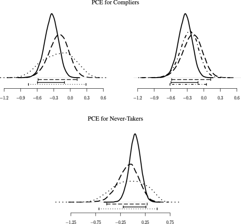
Figure 1: Posterior densities (derived using a kernel smoothing) and 95% posterior intervals of PCEs on depression for compliers ($\tau_{c}$) and never-takers ($\tau_{n}$) under the univariate approach with ER (dot-dashed lines), the univariate approach without ER (dashed lines), the bivariate approach (solid lines) and the bivariate approach with PER (dotted lines).

For the PCEs for compliers, $\tau_{c}$, a negative point estimate is obtained from all four models: $-0.338$ in the bivariate case, $-0.205$ in the bivariate case with PER, $-0.206$ in the univariate case, and $-0.260$ in the univariate case with ER. The posterior probability of this effect being negative is greater than 75% irrespective of the approach we consider. Therefore, all the approaches show some evidence that the invitation to attend the job-search seminars reduces depression among compliers. However, only the bivariate model leads to a 95% credible interval not covering 0, with a 99.8% posterior probability that $\tau_{c}$ is negative. In fact, the bivariate analysis without PER provides considerably more precise estimates for $\tau_{c}$ than both the bivariate analysis with PER and the univariate analyses with and without ER: the bivariate model without ER for any outcomes (row 1) reduces the width of the 95% credible interval for $\tau_{c}$ by $53\%$ compared to the bivariate model with PER (row 2), and by $31\%$ and $26\%$ compared to the univariate model without (row 3) and with (row 4) ER, respectively. This is further illustrated by the posterior densities plotted in the upper panel in Figure 1. The bivariate approach with PER performs worse than the univariate approaches, too: the 95% posterior credible intervals for the PCEs on depression from the bivariate approach with PER are more than 30% wider than those derived from the univariate approaches. Somewhat surprisingly, the posterior distributions of $\tau_{c}$ and $\tau_{n}$ from the model with PER have large variances. This highlights an interesting phenomenon about PER that will be further investigated through our simulations: PER helps to reduce posterior uncertainty only if it does (or approximately) hold and is imposed. However, when it is imposed but does not hold, PER may force the parameters to lie in a region of the natural parameter space that is far away from the truth and thus leads to larger posterior variances. This is what may have happened in the JOBS II analysis: even if there is large posterior uncertainty about the effect of assignment on re-employment for never-takers, imposing this effect to be exactly zero leads to ill-fitted models.

It is worth noting that the bivariate approach leads to posterior distributions of $\tau_{c}$ and $\tau_{n}$ centered at slightly different medians. In light of the simulation results, which show that jointly modeling two outcomes generally leads to posterior means and medians closer to the true values, these findings suggest the bivariate estimates are more reliable, while the univariate estimates may be far from the true values.

JOBS II is a randomized experiment, and so pre-treatment covariates do not enter the assignment mechanism. Nevertheless, covariates could be still used to improve precision of the causal estimates. Our analysis can also use covariates in addition to auxiliary outcomes. Indeed, we also estimated the models previously described conditional on several relevant covariates. Similar results were obtained, but the benefits of the bivariate approach, that we want to highlight here, are particularly evident when no covariates are used. Therefore, we relegate the details for the models with covariates to the supplementary material [Mattei, Li and Mealli (2013)].

5 Simulations

To better understand the results of the JOBS II application and, more importantly, to further shed light on the comparison between univariate and bivariate principal stratification analyses in general settings, we conduct an extensive simulation study. We consider a wide range of simulation scenarios that often occur in practice, accounting for different correlation structures between the outcomes for compliers and never-takers, various deviations from the PER for the secondary outcome, and different association levels between the auxiliary variable and the compliance status.

Table 3: True values of parameters of the seven simulation scenarios. The last two columns show the ratio of the between-groups variance and the total variance of the secondary outcome under the control and the active treatment arm, where the groups are defined by the compliance status (correlation ratio)

Scenario	$\bolds{\mu^{n,0}}$	$\bolds{\mu^{n,1}}$	$\bolds{\Sigma^{n,0}}$	$\bolds{\Sigma^{n,1}}$	$\bolds{\eta^{2}_{Y_{2}|S,Z=0}}$	$\bolds{\eta^{2}_{Y_{2}|S,Z=1}}$
I	$\left[\matrix{2.75\cr 12}\right]$	$\left[\matrix{4.25\cr 12}\right]$	$\left[\matrix{0.16&0.16\cr 0.16&4}\right]$	$\left[\matrix{0.04&0.08\cr 0.08&4}\right]$	$0.639$	$0.770$
II			$\left[\matrix{0.16&0.64\cr 0.64&4}\right]$	$\left[\matrix{0.04&0.32\cr 0.32&4}\right]$
	$\left[\matrix{2.75\cr 12}\right]$	$\left[\matrix{4.25\cr 13}\right]$			$0.639$	$0.824$
III			$\left[\matrix{0.16&0.16\cr 0.16&4}\right]$	$\left[\matrix{0.04&0.08\cr 0.08&4}\right]$
IV			$\left[\matrix{0.16&0.64\cr 0.64&4}\right]$	$\left[\matrix{0.04&0.48\cr 0.48&9}\right]$
	$\left[\matrix{2.75\cr 12}\right]$	$\left[\matrix{4.25\cr 24}\right]$			$0.639$	$0.950$
V			$\left[\matrix{0.16&0.16\cr 0.16&4}\right]$	$\left[\matrix{0.04&0.12\cr 0.12&9}\right]$
VI			$\left[\matrix{0.16&0.96\cr 0.96&9}\right]$	$\left[\matrix{0.04&0.80\cr 0.8&25}\right]$
	$\left[\matrix{2.75\cr 24}\right]$	$\left[\matrix{4.25\cr 36}\right]$			$0.941$	$0.957$
VII			$\left[\matrix{0.16&0.24\cr 0.24&9}\right]$	$\left[\matrix{0.04&0.20\cr 0.2&25}\right]$
In all the scenarios
${\bolds\mu}^{c,0}=\left[\matrix{2.5\cr 8}\right]$, ${\bolds\mu}^{c,1}=\left[\matrix{0.5\cr 6.5}\right]$, ${\bolds\Sigma}^{c,0}=\left[\matrix{0.09&0.24\cr 0.24&1}\right]$, ${\bolds\Sigma}^{c,1}=\left[\matrix{0.01&0.08\cr 0.08&1}\right]$

To simplify computation, we generate two continuous outcomes from a mixture of two bivariate normal distributions as model (4), and the stratum membership from a Bernoulli distribution as model (5). Although we only consider bivariate Normal distributions in our simulations, we can reasonably expect that our results are not tied to distributional assumptions: Mealli and Pacini (2013) show that secondary outcomes can also tighten large-sample nonparametric bounds for PCEs, and Mercatanti, Li and Mealli (2012) show that the use of an auxiliary variable may improve inference also in misspecified Gaussian mixture models. See also, for example, Gallop et al. (2009), Mealli and Pacini (2008), for further insights on the role of distributional assumptions in PS analysis. We assume that parameters are a priori independent and use conjugate diffuse prior distributions. The true simulation parameters are shown in Table 3. Mimicking the JOBS II data, all simulated data sets have $n=600$ units, generated using principal strata probabilities of $0.7$ for compliers and $0.3$ for never-takers. The simulated samples are randomly divided into two groups, half assigned to the treatment and half to the control. Three parallel MCMC chains of 15,000 iterations with different starting values were run for each of the seven simulated data sets, with the first 5000 as burn-in. Mixing of the chains was determined to be adequate and all chains led to similar posterior summary statistics.

Figure 2 shows the posterior densities and 95% posterior credible intervals of the PCEs for compliers and never-takers on the primary outcome, in both the univariate and bivariate cases. The results clearly demonstrate that simultaneous modeling of both outcomes significantly reduces posterior uncertainty for the causal estimates. In fact, the bivariate approach outperforms the univariate one in each of the scenarios considered, providing considerably more precise estimates of the PCEs for compliers and never-takers.

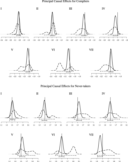
Figure 2: Posterior densities (derived using a kernel smoothing) and 95% posterior intervals of PCEs on the primary outcome for compliers ($\tau_{c}$) and never-takers ($\tau_{n}$) under the univariate approach (dashed lines), the bivariate approach (solid lines) and the bivariate approach with PER (dotted lines). The black vertical lines represent the true values. The Roman numbers denote the simulation scenarios described in Table 3.

The benefits of the bivariate approach especially arise when compliers and never-takers are characterized by different correlation structures (scenarios III and V) and when the association between the auxiliary outcome and the compliance status is stronger (scenarios VI and VII). In addition, plots (III), (V), (VI) and (VII) in the upper and lower panels of Figure 2 suggest that the posterior distributions of the PCEs are much more informative in the bivariate case. Specifically, plots (III) and (VII) show that the posterior distributions of the PCEs for compliers and never-takers are flat in the univariate approach, but become much tighter in the bivariate case. The improvement is even more dramatic in scenarios (V) and (VI), where the plots show that posterior distributions of the PCEs for compliers and never-takers are bimodal in the univariate case, but both become unimodal in the bivariate case. Also, in the above scenarios jointly modeling the two outcomes leads to posterior means of the PCEs for compliers and never-takers much closer to the true values. The bivariate approach outperforms the univariate one also in scenarios II and IV, where compliers and never-takers are characterized by similar correlation structures. In both scenarios the bivariate approach considerably increases the precision of the estimates.

In scenario I, where PER for the secondary outcome holds, we also derived the posterior distributions of the PCEs for compliers and never-takers by specifying a bivariate model that assumes PER. The bivariate models with and without PER lead to similar results, and both clearly outperform the univariate model, leading to much less variable and more informative posterior distributions of the causal effects of interest. Several other scenarios with additional structural assumptions were also examined: magnitude of the improvement varies, but the pattern is consistent with what is described here.

Additional bivariate analyses were conducted to investigate the role of PER, by fitting the bivariate model with PER also to the six data sets generated under scenarios II through VII, where PER does not hold. Results, shown in the supplementary material [Mattei, Li and Mealli (2013)], suggest that inference for the PCE for compliers is robust with respect to violation of PER: the corrected-specified bivariate model and the misspecified bivariate model with PER perform similarly, leading to posterior distributions for the PCE for compliers characterized by similar posterior variability and similar posterior means. On the other hand, inference on the PCE for never-takers appears to be rather sensitive to the PER assumption, especially when PER is strongly violated (scenarios V, VI and VII) and when compliers and never-taker are characterized by similar correlation structures (scenarios II and IV). In these scenarios, the posterior distributions from the misspecified bivariate models with PER are characterized by larger posterior uncertainty and are centered at posterior means much farther away from the true parameters than the posterior means from the corrected-specified bivariate models. Also, the posterior distributions of the PCE for never-takers derived from the misspecified bivariate models with PER provide 95% posterior credible intervals that do not even cover the true parameter in most of the scenarios.

These results shed light on two key complementary facts about PER. First, as already anticipated, PER may help to reduce posterior uncertainty when it does hold and is imposed, although the jointly modeling of two outcomes still improves inference increasing precision, even if no exclusion restriction on the secondary outcome is imposed. It is worth noting that this is a different result from the nonparametric large-sample case, where the secondary outcome does not help sharpening inference if no exclusion restriction is imposed on it [Mealli and Pacini (2013)]. Second, PER may actually increase the posterior variability of the causal estimates and lead to misleading results, when it is imposed but does not hold. Therefore, less precise inference under PER can be viewed as evidence of violation of PER, which is the case in the JOBS II application. This highlights the importance of carefully evaluating the plausibility of ER assumptions.

In order to evaluate the accuracy and robustness of the proposed approach, we also investigated its repeated sampling properties using Monte Carlo simulations, which were summarized by calculating standard frequentist measures, including average biases, percent biases, mean square errors (MSEs) and coverage of nominal 95% confidence intervals. Results [shown in the supplementary material Mattei, Li and Mealli (2013)] confirm, and generally magnify, the findings discussed here that the simultaneous modeling of two outcomes may improve estimation by reducing posterior uncertainty for causal estimands.

6 Posterior predictive model checking

The use of multiple outcomes may help in improving inference, although the additional information provided by secondary outcomes is obtained at the cost of having to specify more complex multivariate models, which may increase the possibility of misspecification. Therefore, model checking procedures to ensure sensible model specification are crucial.

Bayesian goodness-of-fit methods have been proposed in the literature, including Bayes factors and marginal likelihood [e.g., Chib (1995)] and posterior predictive checks [e.g., Rubin (1984), Gelman, Meng and Stern (1996)]. Here, we focus on posterior predictive checks, which are based on comparisons of the observed data to the posterior predictive distribution. A posterior predictive check generally involves the following: (a) choosing a discrepancy measure, $\Delta$; and (b) computing a Bayesian $p$-value.

The posterior predictive discrepancy measures that we use here were first proposed by Barnard et al. (2003) and can be defined as follows. Let ${\mathcal{D}}^{\mathrm{study}}_{s,z}=\{i\dvtx S^{\mathrm{study}}_{i}=s\mbox{ and }Z_{i}=z\}$ be the group of subjects of type $S^{\mathrm{study}}_{i}=s$ assigned to treatment $Z_{i}=z$, $s=c,n$, $z=0,1$, in the $\mathit{study}$ data, where $\mathrm{study}=\mathrm{obs}$ for the observed data and $\mathrm{study}=\mathrm{rep}$ for data from a replicated study, that is, outcome data and compliance status drawn from their joint posterior predictive distribution. Note that the assignment variable is fixed at its observed values. Let $N^{\mathrm{study}}_{s,z}$ be the number of units in the study data belonging to the ${\mathcal{D}}^{\mathrm{study}}_{s,z}$ group, and let $\overline{Y}_{m,s,z}^{\mathrm{study}}$ and $s_{m,s,z}^{2,\mathrm{study}}$ denote the mean and the variance of the outcome variable $Y_{m}^{\mathrm{study}}$, $m=1,2$, for this group of units. Then, the discrepancy measures we use are

$$\mathit{SI}_{m,s}^{\mathrm{study}}(\bolds{\theta}) = \bigl{|}\overline{Y}_{m,s,1}^{\mathrm{study}}-\overline{Y}_{m,s,0}^{\mathrm{study}}\bigr{|}\quad\mathrm{and}$$

$$\mathit{NO}_{m,s}^{\mathrm{study}}(\bolds{\theta}) = \sqrt{\frac{s_{m,s,0}^{2,study}}{N^{\mathrm{study}}_{s,0}}+\frac{s_{m,s,1}^{2,study}}{N^{\mathrm{study}}_{s,1}}}$$

and the ratio of $\mathit{SI}_{m,s}^{\mathrm{study}}(\bolds{\theta})$ to $\mathit{NO}_{m,s}^{\mathrm{study}}(\bolds{\theta})$: $SN_{m,s}^{\mathrm{study}}(\bolds{\theta})=\frac{\mathit{SI}_{m,s}^{\mathrm{study}}(\theta)}{\mathit{NO}_{m,s}^{\mathrm{study}}(\theta)}$, $m=1,2$, $s=c,n$. These measures aim at assessing whether the model, which includes the prior distribution as well as the likelihood, can preserve broad features of signal, $\mathit{SI}_{m,s}^{\mathrm{study}}(\bolds{\theta})$, noise, $\mathit{NO}_{m,s}^{\mathrm{study}}(\bolds{\theta})$, and signal to noise, $SN_{m,s}^{\mathrm{study}}(\bolds{\theta})$, in the outcome distributions for compliers and never-takers.

In order to assess the plausibility of the posited models as a whole, we also consider the $\chi^{2}$ discrepancy, defined as the sum of squares of standardized residuals of the data with respect to their expectations under the posited model [e.g., Gelman, Meng and Stern (1996)]; and for the continuous outcome (depression, $Y_{1}$), the Kolmogorov–Smirnov discrepancy, defined as the maximum difference between the empirical distribution function and the theoretical distribution implied by the posited model.

A widely-used Bayesian $p$-value is the posterior predictive $p$-value(PPPV)—the probability over the posterior predictive distribution of the compliance status and the parameters $\bolds{\theta}$ that a discrepancy measure in a replicated data drawn with the same $\bolds{\theta}$ as in the observed data, $\Delta^{\mathrm{rep}}(\mathbf{S}^{\mathrm{rep}},\bolds{\theta})$, would be as or more extreme than the realized value of that discrepancy measure in the observed study, $\Delta^{\mathrm{obs}}(\mathbf{S}^{\mathrm{obs}},\theta)$: $p(\Delta^{\mathrm{rep}}(\mathbf{S}^{\mathrm{rep}},\bolds{\theta})>\Delta^{\mathrm{obs}}(\mathbf{S}^{\mathrm{obs}},\bolds{\theta})|\break\mathbf{Y}^{\mathrm{obs}},\mathbf{D}^{\mathrm{obs}},\mathbf{Z}^{\mathrm{obs}},\mathbf{X})$ [Rubin (1984), Gelman, Meng and Stern (1996)].

PPPVs are Bayesian posterior probability statements about what might be expected in future replications, conditional on the observed data and the model. Therefore, extreme $p$-values, that is, $p$-values very close either to $0$ or $1$, can be interpreted as evidence that the model cannot capture some aspects of the data described by the corresponding discrepancy measures, and would indicate an undesirable influence of the model in estimation of the estimands of interest.

Although the PPPVs are Bayesian posterior probabilities, even within the Bayesian framework, it is desirable that they are, at least asymptotically, uniformly distributed over hypothetical observed data sets drawn from the true model. Unfortunately, PPPVs are not generally asymptotically uniform, but they tend to be conservative in the sense that the probability of extreme values might be lower than the nominal probabilities from the uniform distribution. This conservatism property implies that PPPVs may lack of power to detect model violations. Alternative posterior predictive checks have been proposed in the literature, including partial posterior predictive $p$-values and conditional predictive $p$-values [e.g., Bayarri and Berger (2000)], calibrated posterior $p$-values [Hjort, Dahl and Steinbakk (2006)] and sampled posterior $p$-values [Johnson (2004, 2007), Gosselin (2011)]. Here we focus on sampled posterior $p$-values (SPPVs), which have been shown to have at least asymptotically a uniform probability distribution [Gosselin (2011)].

The SPPV is defined as $p(\Delta^{\mathrm{rep}}(\mathbf{S}^{\mathrm{rep}},\bolds{\theta}^{(j*)})>\Delta^{\mathrm{obs}}(\mathbf{S}^{\mathrm{obs}},\bolds{\theta}^{(j*)})|\mathbf{Y}^{\mathrm{obs}},\mathbf{D}^{\mathrm{obs}},\break\mathbf{Z}^{\mathrm{obs}},\bolds{\theta}^{(j*)})$, where $\bolds{\theta}^{(j*)}$ is a unique value of $\bolds{\theta}$, randomly sampled from its posterior distribution. Following Gosselin (2011), we calculated the SPPV associated to the JOBS II study using the following two steps: (i) draw $K$ simulated replicated data sets from the sampling distribution conditional on $\bolds{\theta}^{(j*)}$; (ii) draw at random the $p$-value from a Beta distribution with parameters $a+1$ and $b+1$, where

$$a = \sum_{k=1}^{K}\mathbf{1}_{\{\Delta^{\mathrm{rep}_{k}}(\mathbf{S}^{\mathrm{rep}_{k}},\bolds{\theta}^{(j*)})>\Delta^{\mathrm{obs}}(\mathbf{S}^{\mathrm{obs}},\bolds{\theta}^{(j*)})\}}$$

$${}+\varepsilon\sum_{k=1}^{K}\mathbf{1}_{\{\Delta^{\mathrm{rep}_{k}}(\mathbf{S}^{\mathrm{rep}_{k}},\bolds{\theta}^{(j*)})=\Delta^{\mathrm{obs}}(\mathbf{S}^{\mathrm{obs}},\bolds{\theta}^{(j*)})\}},$$

$$b = \sum_{k=1}^{K}\mathbf{1}_{\{\Delta^{\mathrm{rep}_{k}}(\mathbf{S}^{\mathrm{rep}_{k}},\bolds{\theta}^{(j*)})<D^{\mathrm{obs}}(\mathbf{S}^{\mathrm{obs}},\theta^{(j*)})\}}$$

$${}+(1-\varepsilon)\sum_{k=1}^{K}\mathbf{1}_{\{\Delta^{\mathrm{rep}_{k}}(\mathbf{S}^{\mathrm{rep}_{k}},\bolds{\theta}^{(j*)})=\Delta^{\mathrm{obs}}(\mathbf{S}^{\mathrm{obs}},\bolds{\theta}^{(j*)})\}}$$

with $\varepsilon\sim U(0,1)$.

A potential drawback of SPPVs is that they might provide different random results on the same data and the same model, depending on the single value $\bolds{\theta}^{(j*)}$ of the parameter vector $\bolds{\theta}$ that is sampled. To avoid this issue, we also implemented the solution proposed by Gosselin (2011), which involves drawing more than a single value of the parameter vector $\bolds{\theta}$ from its posterior distribution. The steps are as follows: (a) a value $u$ from a uniform distribution on $(0,1)$ is drawn; (b) $J>1$ values of the parameter vector $\bolds{\theta}$, $\bolds{\theta}^{(1)},\ldots,\bolds{\theta}^{(J)}$, are drawn from its posterior distribution; (c) for each $j=1,\ldots,J$, the sample posterior $p$-value associated with $\bolds{\theta}^{(j)}$ is computed; (d) the SPPVs are combined using the empirical $u$-quantile of the latter distribution. We call the Bayesian $p$-value derived from this approach the modified-SPPV.

Table 4: Posterior predictive checks

Approach		Signal		Noise		Signal-to-Noise
	Outcome	$\bolds{c}$	$\bolds{n}$	$\bolds{c}$	$\bolds{n}$	$\bolds{c}$	$\bolds{n}$	$\bolds{\chi^{2}}$	Kolmogorov–Smirnov
		Posterior predictive $p$-values
Bivariate
	Depression	0.513	0.805	0.432	0.564	0.528	0.798	0.597	0.400
	Re-employment	0.497	0.502	0.670	0.242	0.416	0.582	0.475
Bivariate with PER
	Depression	0.573	0.574	0.522	0.573	0.562	0.552	0.563	0.389
	Re-employment	0.542	0.493	0.408	0.492	0.545	0.493	0.382
Univariate
	Depression	0.601	0.678	0.836	0.865	0.536	0.623	0.979	0.441
Univariate with ER
	Depression	0.555		0.802		0.484		0.939	0.373
		Sample posterior $p$-values
Bivariate
	Depression	0.545	0.798	0.697	0.619	0.473	0.783	0.866	0.816
	Re-employment	0.379	0.438	0.830	0.121	0.262	0.582	0.663
Bivariate with PER
	Depression	0.693	0.807	0.512	0.520	0.663	0.800	0.592	0.341
	Re-employment	0.856	0.818	0.527	0.341	0.863	0.761	0.416
Univariate
	Depression	0.170	0.731	0.747	0.320	0.154	0.757	0.699	0.410
Univariate with ER
	Depression	0.190		0.625		0.169		0.899	0.392
		Modified sample posterior $p$-values
Bivariate
	Depression	0.893	0.872	0.571	0.367	0.401	0.747	0.803	0.659
	Re-employment	0.228	0.115	0.705	0.618	0.122	0.690	0.433
Bivariate with PER
	Depression	0.117	0.605	0.631	0.542	0.329	0.329	0.546	0.627
	Re-employment	0.495	0.802	0.892	0.260	0.788	0.699	0.566
Univariate
	Depression	0.241	0.283	0.888	0.868	0.820	0.097	0.900	0.255
Univariate with ER
	Depression	0.200		0.811		0.724		0.692	0.172

Table 4 shows the results from the three Bayesian $p$-values we considered. The SPPVs are based on $K=500$ replicated data sets, and the modified-SPPVs were calculated by drawing at random $J=1000$ values of the parameter vector from its (simulated) posterior distribution and simulating $K=500$ replicated data sets for each $j=1,\ldots,J$.

As can be seen in Table 4, the estimated Bayesian $p$-values for the bivariate model that does not assume ER for any outcome range between 11.5% and 89.3%, suggesting that the bivariate model fits the data pretty well and successfully replicates the corresponding measure of location, dispersion and their relative magnitude. Unsurprisingly, similar results are obtained for the bivariate model with PER for re-employment. In fact, the analyses do not provide strong evidence against PER for re-employment, so it is reasonable that posterior predictive checks fail to detect the potential benefits of the bivariate model that does not assume PER over the bivariate model that does assume PER. However, the empirical results in Section 4 show that the bivariate model without PER considerably reduces posterior uncertainty for the causal estimands of interest. Therefore, also in light of the simulations, we expect that inferences drawn without assuming PER may be more reliable. On the other hand, the PPPVs and the modified-SPPVs show some evidence that the univariate models might not optimally fit the data according to the $\chi^{2}$ discrepancy. In addition, the modified-SPPVs suggest that the univariate model without ER might fail to replicate the signal-to-noise measure in the depression distribution for never-takers. These potential failures of the univariate models might be due to the underlying categorical nature of the depression variable. More flexible statistical models could be considered and compared, but the potential failures of the univariate models seem to be successfully fixed when the additional information provided by the secondary outcome is used, so we do not further drill down this issue in this paper, where focus is on investigating the benefits of jointly modeling multiple outcomes in causal inference with post-treatment variables.

7 Conclusion

Motivated by the evaluation of a job training program (JOBS II), we have demonstrated, within the framework of principal stratification, the benefits of jointly modeling more than one outcome in model-based causal analysis for studies with intermediate variables. Observed distributions in these studies are typically mixtures of distributions associated with latent subgroups (principal strata). Structural or behaviorial assumptions are often invoked to uniquely disentangle these mixtures. When such assumptions are not plausible, distributional assumptions are often invoked. But these usually lead to models that are weakly identified, weakly in the sense that the likelihood function has substantial regions of flatness. From a Bayesian perspective, even when the likelihood is rather flat, if the prior is proper, so will be the posterior. However, posterior uncertainty will still be rather large in these models, with posterior distributions of causal parameters often presenting more than a single mode, unless the prior is extremely informative.

We have shown how to sharpen inference in these weakly identified models: improvements are achieved without adding prior information or additional assumptions (such as ERs, weak monotonicity or stochastic dominance), but rather by using the additional information provided by the joint distribution of the outcome of interest with secondary outcomes. Indeed, in the JOBS II application, ERs are not particularly plausible. Nonetheless, by jointly modeling depression, the primary outcome, and re-employment status, a secondary outcome, we have found improved evidence for a positive effect of the job-training program on trainees’ depression compared to a univariate analysis on depression alone. Additional simulations further illustrate the benefits under more general scenarios.

JOBS II is a randomized study, but we stress that our framework can also serve as a template for the analysis of observational studies with intermediate variables. In observational studies, randomization (ignorability) of treatment assignment is usually assumed conditional on relevant pretreatment variables [Rosenbaum and Rubin (1983)], thereby conditioning on the covariates is not optional in observational studies but crucial for credible causal statements. However, once ignorability is assumed, the structure for Bayesian inference in observational studies with intermediate variables (e.g., mediation analysis) is the same as that in randomized experiments. The differences lie in the structural assumptions: for example, while in some experiments the design of the study can help in making the ER assumption plausible (blindness or double-blindness), the ER assumption for an instrument in observational studies is often questionable. As a consequence, improving inference of weakly identified models is even more relevant in observational studies.

References

- Angrist, Imbens and Rubin (1996) {barticle}[auto:STB—2013/10/14—10:36:11] \bauthor\bsnmAngrist, \bfnmJ. D.\binitsJ. D., \bauthor\bsnmImbens, \bfnmG. W.\binitsG. W. and \bauthor\bsnmRubin, \bfnmD. B.\binitsD. B. (\byear1996). \btitleIdentification of causal effects using instrumental variables. \bjournalJ. Amer. Statist. Assoc. \bvolume91 \bpages444–455. \bptokimsref \endbibitem
- Barnard et al. (2003) {barticle}[mr] \bauthor\bsnmBarnard, \bfnmJohn\binitsJ., \bauthor\bsnmFrangakis, \bfnmConstantine E.\binitsC. E., \bauthor\bsnmHill, \bfnmJennifer L.\binitsJ. L. and \bauthor\bsnmRubin, \bfnmDonald B.\binitsD. B. (\byear2003). \btitlePrincipal stratification approach to broken randomized experiments: A case study of school choice vouchers in New York City. \bjournalJ. Amer. Statist. Assoc. \bvolume98 \bpages299–323. \biddoi=10.1198/016214503000071, issn=0162-1459, mr=1995712 \bptnotecheck related\bptokimsref \endbibitem
- Bayarri and Berger (2000) {barticle}[mr] \bauthor\bsnmBayarri, \bfnmM. J.\binitsM. J. and \bauthor\bsnmBerger, \bfnmJames O.\binitsJ. O. (\byear2000). \btitle values for composite null models. \bjournalJ. Amer. Statist. Assoc. \bvolume95 \bpages1127–1142. \biddoi=10.2307/2669749, issn=0162-1459, mr=1804239 \bptnotecheck related\bptokimsref \endbibitem
- Chib (1995) {barticle}[mr] \bauthor\bsnmChib, \bfnmSiddhartha\binitsS. (\byear1995). \btitleMarginal likelihood from the Gibbs output. \bjournalJ. Amer. Statist. Assoc. \bvolume90 \bpages1313–1321. \bidissn=0162-1459, mr=1379473 \bptokimsref \endbibitem
- Chib and Hamilton (2000) {barticle}[auto:STB—2013/10/14—10:36:11] \bauthor\bsnmChib, \bfnmS.\binitsS. and \bauthor\bsnmHamilton, \bfnmB. H.\binitsB. H. (\byear2000). \btitleBayesian analysis of cross-section and clustered data treatment models. \bjournalJ. Econometrics \bvolume97 \bpages25–50. \bptokimsref \endbibitem
- Elliott, Raghunathan and Li (2010) {barticle}[pbm] \bauthor\bsnmElliott, \bfnmMichael R.\binitsM. R., \bauthor\bsnmRaghunathan, \bfnmTrivellore E.\binitsT. E. and \bauthor\bsnmLi, \bfnmYun\binitsY. (\byear2010). \btitleBayesian inference for causal mediation effects using principal stratification with dichotomous mediators and outcomes. \bjournalBiostatistics \bvolume11 \bpages353–372. \biddoi=10.1093/biostatistics/kxp060, issn=1468-4357, pii=kxp060, pmcid=2830580, pmid=20101045 \bptokimsref \endbibitem
- Frangakis and Rubin (2002) {barticle}[mr] \bauthor\bsnmFrangakis, \bfnmConstantine E.\binitsC. E. and \bauthor\bsnmRubin, \bfnmDonald B.\binitsD. B. (\byear2002). \btitlePrincipal stratification in causal inference. \bjournalBiometrics \bvolume58 \bpages21–29. \biddoi=10.1111/j.0006-341X.2002.00021.x, issn=0006-341X, mr=1891039 \bptokimsref \endbibitem
- Gallop et al. (2009) {barticle}[mr] \bauthor\bsnmGallop, \bfnmRobert\binitsR., \bauthor\bsnmSmall, \bfnmDylan S.\binitsD. S., \bauthor\bsnmLin, \bfnmJulia Y.\binitsJ. Y., \bauthor\bsnmElliott, \bfnmMichael R.\binitsM. R., \bauthor\bsnmJoffe, \bfnmMarshall\binitsM. and \bauthor\bsnmTen Have, \bfnmThomas R.\binitsT. R. (\byear2009). \btitleMediation analysis with principal stratification. \bjournalStat. Med. \bvolume28 \bpages1108–1130. \biddoi=10.1002/sim.3533, issn=0277-6715, mr=2662200 \bptokimsref \endbibitem
- Gelman, Meng and Stern (1996) {barticle}[mr] \bauthor\bsnmGelman, \bfnmAndrew\binitsA., \bauthor\bsnmMeng, \bfnmXiao-Li\binitsX.-L. and \bauthor\bsnmStern, \bfnmHal\binitsH. (\byear1996). \btitlePosterior predictive assessment of model fitness via realized discrepancies. \bjournalStatist. Sinica \bvolume6 \bpages733–807. \bidissn=1017-0405, mr=1422404 \bptnotecheck related\bptokimsref \endbibitem
- Gelman and Rubin (1992) {barticle}[auto:STB—2013/10/14—10:36:11] \bauthor\bsnmGelman, \bfnmA. E.\binitsA. E. and \bauthor\bsnmRubin, \bfnmD. B.\binitsD. B. (\byear1992). \btitleInference from iterative simulation using multiple sequences. \bjournalStatist. Sci. \bvolume7 \bpages457–472. \bptokimsref \endbibitem
- Gilbert and Hudgens (2008) {barticle}[mr] \bauthor\bsnmGilbert, \bfnmPeter B.\binitsP. B. and \bauthor\bsnmHudgens, \bfnmMichael G.\binitsM. G. (\byear2008). \btitleEvaluating candidate principal surrogate endpoints. \bjournalBiometrics \bvolume64 \bpages1146–1154. \biddoi=10.1111/j.1541-0420.2008.01014.x, issn=0006-341X, mr=2522262 \bptokimsref \endbibitem
- Gosselin (2011) {barticle}[auto:STB—2013/10/14—10:36:11] \bauthor\bsnmGosselin, \bfnmF.\binitsF. (\byear2011). \btitleA new calibrated Bayesian internal goodness-of-fit method: Sampled posterior -values as simple and general -values that allow double use of the data. \bjournalPLoS ONE \bvolume6 \bpages1–10. \bptokimsref \endbibitem
- Gustafson (2009) {barticle}[mr] \bauthor\bsnmGustafson, \bfnmPaul\binitsP. (\byear2009). \btitleWhat are the limits of posterior distributions arising from nonidentified models and why should we care? \bjournalJ. Amer. Statist. Assoc. \bvolume104 \bpages1682–1695. \biddoi=10.1198/jasa.2009.tm08603, issn=0162-1459, mr=2750585 \bptokimsref \endbibitem
- Hirano et al. (2000) {barticle}[auto:STB—2013/10/14—10:36:11] \bauthor\bsnmHirano, \bfnmK.\binitsK., \bauthor\bsnmImbens, \bfnmG. W.\binitsG. W., \bauthor\bsnmRubin, \bfnmD. B.\binitsD. B. and \bauthor\bsnmZhou, \bfnmX. H.\binitsX. H. (\byear2000). \btitleAssessing the effect of an influenza vaccine in an encouragement design. \bjournalBiostatistics \bvolume1 \bpages69–88. \bptokimsref \endbibitem
- Hjort, Dahl and Steinbakk (2006) {barticle}[mr] \bauthor\bsnmHjort, \bfnmNils Lid\binitsN. L., \bauthor\bsnmDahl, \bfnmFredrik A.\binitsF. A. and \bauthor\bsnmSteinbakk, \bfnmGunnhildur Högnadóttir\binitsG. H. (\byear2006). \btitlePost-processing posterior predictive -values. \bjournalJ. Amer. Statist. Assoc. \bvolume101 \bpages1157–1174. \biddoi=10.1198/016214505000001393, issn=0162-1459, mr=2324154 \bptokimsref \endbibitem
- Imbens and Rubin (1997) {barticle}[mr] \bauthor\bsnmImbens, \bfnmGuido W.\binitsG. W. and \bauthor\bsnmRubin, \bfnmDonald B.\binitsD. B. (\byear1997). \btitleBayesian inference for causal effects in randomized experiments with noncompliance. \bjournalAnn. Statist. \bvolume25 \bpages305–327. \biddoi=10.1214/aos/1034276631, issn=0090-5364, mr=1429927 \bptokimsref \endbibitem
- Jin and Rubin (2008) {barticle}[mr] \bauthor\bsnmJin, \bfnmHui\binitsH. and \bauthor\bsnmRubin, \bfnmDonald B.\binitsD. B. (\byear2008). \btitlePrincipal stratification for causal inference with extended partial compliance. \bjournalJ. Amer. Statist. Assoc. \bvolume103 \bpages101–111. \biddoi=10.1198/016214507000000347, issn=0162-1459, mr=2463484 \bptokimsref \endbibitem
- Jo and Muthen (2001) {bincollection}[auto:STB—2013/10/14—10:36:11] \bauthor\bsnmJo, \bfnmB.\binitsB. and \bauthor\bsnmMuthen, \bfnmB.\binitsB. (\byear2001). \btitleModeling of intervention effects with noncompliance: A latent variable approach for randomized trials. In \bbooktitleNew developments and techniques in structrual equation modeling (\beditor\binitsG. A.\bfnmG. A. \bsnmMarcoulides and \beditor\binitsR. E.\bfnmR. E. \bsnmSchumacker, eds.) \bpages57–87. \bpublisherErlbaum Associates, \baddressMahwah, NJ. \bptokimsref \endbibitem
- Johnson (2004) {barticle}[mr] \bauthor\bsnmJohnson, \bfnmValen E.\binitsV. E. (\byear2004). \btitleA Bayesian test for goodness-of-fit. \bjournalAnn. Statist. \bvolume32 \bpages2361–2384. \biddoi=10.1214/009053604000000616, issn=0090-5364, mr=2153988 \bptokimsref \endbibitem
- Johnson (2007) {barticle}[mr] \bauthor\bsnmJohnson, \bfnmValen E.\binitsV. E. (\byear2007). \btitleBayesian model assessment using pivotal quantities. \bjournalBayesian Anal. \bvolume2 \bpages719–733. \biddoi=10.1214/07-BA229, issn=1931-6690, mr=2361972 \bptokimsref \endbibitem
- Li, Taylor and Elliott (2010) {barticle}[mr] \bauthor\bsnmLi, \bfnmYun\binitsY., \bauthor\bsnmTaylor, \bfnmJeremy M. G.\binitsJ. M. G. and \bauthor\bsnmElliott, \bfnmMichael R.\binitsM. R. (\byear2010). \btitleA Bayesian approach to surrogacy assessment using principal stratification in clinical trials. \bjournalBiometrics \bvolume66 \bpages523–531. \biddoi=10.1111/j.1541-0420.2009.01303.x, issn=0006-341X, mr=2758832 \bptokimsref \endbibitem
- Li, Taylor and Elliott (2011) {barticle}[auto:STB—2013/10/14—10:36:11] \bauthor\bsnmLi, \bfnmY.\binitsY., \bauthor\bsnmTaylor, \bfnmJ. M. G.\binitsJ. M. G. and \bauthor\bsnmElliott, \bfnmM. R.\binitsM. R. (\byear2011). \btitleCausal assessment of surrogacy in a metanalysis of colorectal cancer trials. \bjournalBiostatistics \bvolume12 \bpages478–492. \bptokimsref \endbibitem
- Little and Yau (1998) {barticle}[auto:STB—2013/10/14—10:36:11] \bauthor\bsnmLittle, \bfnmR. J.\binitsR. J. and \bauthor\bsnmYau, \bfnmL. H. Y.\binitsL. H. Y. (\byear1998). \btitleStatistical techniques for analyzing data from prevention trials: Treatment of no-shows using Rubin’s causal model. \bjournalPsychological Methods \bvolume3 \bpages147–159. \bptokimsref \endbibitem
- Manski (1990) {barticle}[auto:STB—2013/10/14—10:36:11] \bauthor\bsnmManski, \bfnmC. F.\binitsC. F. (\byear1990). \btitleNonparametric bounds on treatment effects. \bjournalThe American Economic Review \bvolume80 \bpages319–323. \bptokimsref \endbibitem
- Mattei, Li and Mealli (2013) {bmisc}[auto:STB—2013/10/14—10:36:11] \bauthor\bsnmMattei, \bfnmA.\binitsA., \bauthor\bsnmLi, \bfnmF.\binitsF. and \bauthor\bsnmMealli, \bfnmF.\binitsF. (\byear2013). \bhowpublishedSupplement to “Exploiting multiple outcomes in Bayesian principal stratification analysis with application to the evaluation of a job training program.” DOI:\doiurl10.1214/13-AOAS674SUPP. \bptokimsref \endbibitem
- Mattei and Mealli (2007) {barticle}[mr] \bauthor\bsnmMattei, \bfnmA.\binitsA. and \bauthor\bsnmMealli, \bfnmF.\binitsF. (\byear2007). \btitleApplication of the principal stratification approach to the Faenza randomized experiment on breast self-examination. \bjournalBiometrics \bvolume63 \bpages437–446. \biddoi=10.1111/j.1541-0420.2006.00684.x, issn=0006-341X, mr=2370802 \bptokimsref \endbibitem
- Mealli and Pacini (2008) {barticle}[mr] \bauthor\bsnmMealli, \bfnmFabrizia\binitsF. and \bauthor\bsnmPacini, \bfnmBarbara\binitsB. (\byear2008). \btitleComparing principal stratification and selection models in parametric causal inference with nonignorable missingness. \bjournalComput. Statist. Data Anal. \bvolume53 \bpages507–516. \biddoi=10.1016/j.csda.2008.09.005, issn=0167-9473, mr=2649105 \bptnotecheck year\bptokimsref \endbibitem
- Mealli and Pacini (2013) {barticle}[auto:STB—2013/10/14—10:36:11] \bauthor\bsnmMealli, \bfnmF.\binitsF. and \bauthor\bsnmPacini, \bfnmB.\binitsB. (\byear2013). \btitleUsing secondary outcomes and covariates to sharpen inference in randomized experiments with noncompliance. \bjournalJ. Amer. Statist. Assoc. \bvolume108 \bpages1120–1131. \bptokimsref \endbibitem
- Mercatanti, Li and Mealli (2012) {bmisc}[auto:STB—2013/10/14—10:36:11] \bauthor\bsnmMercatanti, \bfnmA.\binitsA., \bauthor\bsnmLi, \bfnmF.\binitsF. and \bauthor\bsnmMealli, \bfnmF.\binitsF. (\byear2012). \bhowpublishedImproving inference of Gaussian mixtures using auxiliary variables. Discussion Paper 12–14. Dept. Statistical Science, Duke Univ., Durham, NC. \bptokimsref \endbibitem
- Rosenbaum (1984) {barticle}[auto:STB—2013/10/14—10:36:11] \bauthor\bsnmRosenbaum, \bfnmP. R.\binitsP. R. (\byear1984). \btitleThe consequences of adjustment for a concomitant variable that has been affected by the treatment. \bjournalJ. Roy. Statist. Soc. Ser. A \bvolume147 \bpages656–666. \bptokimsref \endbibitem
- Rosenbaum and Rubin (1983) {barticle}[mr] \bauthor\bsnmRosenbaum, \bfnmPaul R.\binitsP. R. and \bauthor\bsnmRubin, \bfnmDonald B.\binitsD. B. (\byear1983). \btitleThe central role of the propensity score in observational studies for causal effects. \bjournalBiometrika \bvolume70 \bpages41–55. \biddoi=10.1093/biomet/70.1.41, issn=0006-3444, mr=0742974 \bptokimsref \endbibitem
- Rubin (1974) {barticle}[auto:STB—2013/10/14—10:36:11] \bauthor\bsnmRubin, \bfnmD. B.\binitsD. B. (\byear1974). \btitleEstimating causal effects of treatments in randomized and nonrandomized studies. \bjournalJournal of Educational Psychology \bvolume66 \bpages688–701. \bptokimsref \endbibitem
- Rubin (1978) {barticle}[mr] \bauthor\bsnmRubin, \bfnmDonald B.\binitsD. B. (\byear1978). \btitleBayesian inference for causal effects: The role of randomization. \bjournalAnn. Statist. \bvolume6 \bpages34–58. \bidissn=0090-5364, mr=0472152 \bptokimsref \endbibitem
- Rubin (1980) {barticle}[mr] \bauthor\bsnmRubin, \bfnmD. B.\binitsD. B. (\byear1980). \btitleComment on “Randomization analysis of experimental data: The Fisher randomization test” by D. Basu. \bjournalJ. Amer. Statist. Assoc. \bvolume75 \bpages591–593. \bidissn=0003-1291, mr=0590687 \bptnotecheck related\bptokimsref \endbibitem
- Rubin (1984) {barticle}[mr] \bauthor\bsnmRubin, \bfnmDonald B.\binitsD. B. (\byear1984). \btitleBayesianly justifiable and relevant frequency calculations for the applied statistician. \bjournalAnn. Statist. \bvolume12 \bpages1151–1172. \biddoi=10.1214/aos/1176346785, issn=0090-5364, mr=0760681 \bptokimsref \endbibitem
- Schwartz, Li and Mealli (2011) {barticle}[mr] \bauthor\bsnmSchwartz, \bfnmScott L.\binitsS. L., \bauthor\bsnmLi, \bfnmFan\binitsF. and \bauthor\bsnmMealli, \bfnmFabrizia\binitsF. (\byear2011). \btitleA Bayesian semiparametric approach to intermediate variables in causal inference. \bjournalJ. Amer. Statist. Assoc. \bvolume106 \bpages1331–1344. \biddoi=10.1198/jasa.2011.ap10425, issn=0162-1459, mr=2896839 \bptokimsref \endbibitem
- Schwartz, Li and Reiter (2012) {barticle}[mr] \bauthor\bsnmSchwartz, \bfnmScott\binitsS., \bauthor\bsnmLi, \bfnmFan\binitsF. and \bauthor\bsnmReiter, \bfnmJerome P.\binitsJ. P. (\byear2012). \btitleSensitivity analysis for unmeasured confounding in principal stratification settings with binary variables. \bjournalStat. Med. \bvolume31 \bpages949–962. \biddoi=10.1002/sim.4472, issn=0277-6715, mr=2913871 \bptokimsref \endbibitem
- Sjölander et al. (2009) {barticle}[mr] \bauthor\bsnmSjölander, \bfnmArvid\binitsA., \bauthor\bsnmHumphreys, \bfnmKeith\binitsK., \bauthor\bsnmVansteelandt, \bfnmStijn\binitsS., \bauthor\bsnmBellocco, \bfnmRino\binitsR. and \bauthor\bsnmPalmgren, \bfnmJuni\binitsJ. (\byear2009). \btitleSensitivity analysis for principal stratum direct effects, with an application to a study of physical activity and coronary heart disease. \bjournalBiometrics \bvolume65 \bpages514–520. \biddoi=10.1111/j.1541-0420.2008.01108.x, issn=0006-341X, mr=2751475 \bptokimsref \endbibitem
- Small and Cheng (2009) {barticle}[mr] \bauthor\bsnmSmall, \bfnmDylan S.\binitsD. S. and \bauthor\bsnmCheng, \bfnmJing\binitsJ. (\byear2009). \btitleComment on “Identifiability and estimation of causal effects in randomized trials with noncompliance and completely nonignorable missing data.” \bjournalBiometrics \bvolume65 \bpages682–686. \biddoi=10.1111/j.1541-0420.2008.01121.x, issn=0006-341X, mr=2766612 \bptnotecheck related\bptokimsref \endbibitem
- Sommer and Zeger (1991) {barticle}[pbm] \bauthor\bsnmSommer, \bfnmA.\binitsA. and \bauthor\bsnmZeger, \bfnmS. L.\binitsS. L. (\byear1991). \btitleOn estimating efficacy from clinical trials. \bjournalStat. Med. \bvolume10 \bpages45–52. \bidissn=0277-6715, pmid=2006355 \bptokimsref \endbibitem
- Ten Have et al. (2004) {barticle}[auto:STB—2013/10/14—10:36:11] \bauthor\bsnmTen Have, \bfnmT. R.\binitsT. R., \bauthor\bsnmElliott, \bfnmM. R.\binitsM. R., \bauthor\bsnmJoffe, \bfnmM.\binitsM. and \bauthor\bsnmZanutto, \bfnmE.\binitsE. (\byear2004). \btitleCausal linear models for non-compliance under randomized treatment with univariate continuous response. \bjournalJ. Amer. Statist. Assoc. \bvolume99 \bpages16–25. \bptokimsref \endbibitem
- Vinokur, Caplan and Williams (1987) {barticle}[auto:STB—2013/10/14—10:36:11] \bauthor\bsnmVinokur, \bfnmA. D.\binitsA. D., \bauthor\bsnmCaplan, \bfnmR. D.\binitsR. D. and \bauthor\bsnmWilliams, \bfnmC. C.\binitsC. C. (\byear1987). \btitleEffects of recent and past stress on mental health: Coping with unemployment among Vietnam veterans and non-veterans. \bjournalJournal of Applied Social Psychology \bvolume17 \bpages710–730. \bptokimsref \endbibitem
- Vinokur, Price and Schul (1995) {barticle}[auto:STB—2013/10/14—10:36:11] \bauthor\bsnmVinokur, \bfnmA. D.\binitsA. D., \bauthor\bsnmPrice, \bfnmR. H.\binitsR. H. and \bauthor\bsnmSchul, \bfnmY.\binitsY. (\byear1995). \btitleImpact of the JOBS intervention on unemployed workers varying in risk for depression. \bjournalAmerican Journal of Community Psychology \bvolume23 \bpages39–74. \bptokimsref \endbibitem
- Zhang and Rubin (2003) {barticle}[auto:STB—2013/10/14—10:36:11] \bauthor\bsnmZhang, \bfnmJ. L.\binitsJ. L. and \bauthor\bsnmRubin, \bfnmD. B.\binitsD. B. (\byear2003). \btitleEstimation of causal effects via principal stratification when some outcomes are truncated by “death.” \bjournalJournal of Educational and Behavioral Statistics \bvolume28 \bpages353–368. \bptokimsref \endbibitem