Precession driven flows in non-axisymmetric ellipsoids

Abstract

We study the flow forced by precession in rigid non-axisymmetric ellipsoidal containers. To do so, we revisit the inviscid and viscous analytical models which have been previously developed for the spheroidal geometry by respectively Poincaré [͓Bull. Astron. 27, 321 (1910)] and Busse [J. Fluid Mech. 33, 739 (1968)], and, we report the first numerical simulations of flows in such a geometry. In strong contrast with axisymmetric spheroids where the forced flow is systematically stationary in the precessing frame, we show that the forced flow is unsteady and periodic. Comparisons of the numerical simulations with the proposed theoretical model show excellent agreement for both axisymmetric and non-axisymmetric containers. Finally, since the studied configuration corresponds to a tidally locked celestial body such as the Earth’s Moon, we use our model to investigate the challenging but planetary relevant limit of very small Ekman numbers and the particular case of our Moon.

1 Introduction

1.1 General context

A rotating solid object is said to precess when its rotation axis itself rotates about a secondary axis that is fixed in an inertial frame of reference. The case of a precessing fluid-filled container has been studied for over one century because of its multiple applications. These flows are indeed present in fluid-filled spinning tops Stewartson (1959), gyroscopes, Gans (1984) or tanks of spacecrafts Garg et al. (1986); Agrawal (1993), possibly affecting the spacecraft stability Bao & Pascal (1997). Precession driven flows are also present in planetary fluid layers, such as the liquid core of the Earth Greff-Lefftz & Legros (1999) or the Moon Meyer & Wisdom (2011), where they possibly participate in the dynamo mechanism generating their magnetic fields Bullard (1949); Bondi & Lyttleton (1953); Malkus (1968). These flows may also have an astrophysical relevance, for instance in neutron stars interiors where they can play a role in the observed precession of radio pulsars Glampedakis et al. (2009).

The first theoretical studies considered the case of an inviscid fluid in a spheroidal container Hough (1895); Sloudsky (1895); Poincaré (1910). Assuming a uniform vorticity, they obtained a solution, the so-called Poincaré flow, given by the sum of a solid body rotation and a potential flow. However, the Poincaré solution is modified by the apparition of boundary layers, and some strong internal shear layers are also created in the bulk of the flow Stewartson & Roberts (1963); Busse (1968). These viscous effects have been taken into account as a correction to the inviscid flow in a spheroid, by considering carefully the Ekman layer and its critical regions Busse (1968); Zhang et al. (2010). Beyond this correction approach, the complete viscous solution, including the fine description of all the flow viscous layers, has recently been obtained in the particular case of a spherical container with weak precession Kida (2011).

When the precession forcing is large enough compared to viscous effects, instabilities can occur and destabilize the Poincaré flow. First, the Ekman layers can be destabilized Lorenzani (2001) through standard Ekman layer instabilities Lingwood (1997); Faller (1991). In this case, the instability remains localized near the boundaries. Second, the whole Poincaré flow can be destabilized, leading to a volume turbulence: this is the precessional instability Malkus (1968). This small-scale intermittent flow confirm the possible relevance of precession for energy dissipation or magnetic field generation, and has thus motivated many studies. Early experimental attempts Vanyo (1991); Vanyo et al. (1995) to confirm the theory of Busse (1968) did not give very good results Pais & Le Mouël (2001). Simulations have thus been performed in spherical containers Tilgner (1999); Tilgner & Busse (2001), spheres Noir et al. (2001), and finally in spheroidal containers Lorenzani & Tilgner (2001, 2003), allowing a validation of the theory of Busse (1968). Experimental confirmation of the theory has then been obtained in spheroids Noir et al. (2003), a work followed by many experimental studies involving spheres Goto et al. (2007); Kida & Nakazawa (2010); Boisson et al. (2012), spherical containers Triana et al. (2012), but also cylinders Meunier et al. (2008); Lagrange et al. (2008, 2011).

Finally, the dynamo capability of precession driven flows has then been demonstrated in spheres Tilgner (2005, 2007), spheroids Wu & Roberts (2009) and cylinders Nore et al. (2011), allowing the possibility of a precession driven dynamo in the liquid core of the Earth Kerswell (1996) or the Moon Dwyer et al. (2011).

1.2 Motivations

All the previously cited works have considered axisymmetric geometries. However, in natural systems, both the planet rotation and the gravitational tides deform the celestial body into a triaxial ellipsoid, where the so-called elliptical (or tidal) instability may take place Lacaze et al. (2004); Le Bars et al. (2010); Cébron et al. (2010a). Generally speaking, the elliptical instability can be seen as the inherent local instability of elliptical streamlines Bayly (1986); Waleffe (1990); Le Dizès (2000), or as the parametric resonance between two free inertial waves (resp. modes) of the rotating unbounded (resp. bounded) fluid and an elliptical strain (of azimutal wavenumber $m=2$). Similarly, it has been suggested that the precession instability comes from the parametric resonance of two inertial waves with the forcing related to the precession of azimutal wavenumber $m=1$ in spheroids Kerswell (1993); Wu & Roberts (2009) and in cylinders Lagrange et al. (2008, 2011). However, the precession instability is also observed in spheres where there is no $m=1$ forcing from the container boundary. It has thus been suggested that the precession instability may be related to another mechanism Lorenzani & Tilgner (2001, 2003). Clearly, the precise origin of the precession instability is still under debate, and is beyond the point of the present work. But since tides and precession are simultaneously present in natural systems, it seems necessary to study their reciprocal influence, in presence or not of instabilities.

The full problem is thus rather complex, involving non-axisymmetric geometries and three different rotating frames: the precessing frame, with a period $T_{p}\approx 26\,000$ years for the Earth, the frame of the tidal bulge, with a period around $T_{d}\approx 27$ days for the Earth, and the container or ’mantle’ frame, with a period $T_{s}=23.9$ hours for the Earth. Working in a frame where the geometry is at rest is particularly suitable for theoretical and numerical studies, and this is only possible when two of the three problem timescales are equal. The case $T_{d}=T_{p}$ where the container is fixed in the precessing frame has already been considered Cébron et al. (2010b), with triaxial ellipsoidal (deformable) containers in order to study the interaction between the elliptical instability and the precession. In this work, we rather focus on the case $T_{d}=T_{s}$, which corresponds to rigid precessing containers. This model is thus relevant for fluid layers of terrestrial planets or moons locked in a synchronization state (i.e. $T_{d}=T_{s}$) such as the liquid core of the Moon.

The paper is organized as follows. In section 2, we define the problem and introduce the theoretical inviscid and viscous models considered in this work. Using non-linear viscous three-dimensional simulations, we then validate successfully in section 3 the proposed theoretical viscous model. The results obtained are then discussed (section 4) and applied to the liquid core of the Moon in the conclusion (section 5).

2 Mathematical description of the problem

We consider an incompressible fluid of density $\rho$ and kinematic viscosity $\nu$ enclosed in a triaxial ellipsoid of principal axes $(a,b,c)$. The cavity rotates along its principal axis of length $c$, and precesses along the unit vector $\hat{\boldsymbol{k}}_{p}$, as illustrated in figure 1a. We denote by ${\boldsymbol{\Omega}}_{m}$ the instantaneous total vector of rotation of the cavity in the frame of inertia, ${\boldsymbol{\Omega_{o}}}=\Omega_{o}\hat{\boldsymbol{k}}$ the rotation vector of the cavity in the precessing frame, and ${\boldsymbol{\Omega_{p}}}=\Omega_{p}\,\hat{{\boldsymbol{k}}}_{p}$ the precession vector in the frame of inertia, such that

$${\boldsymbol{\Omega}}_{m}={\boldsymbol{\Omega_{o}}}+{\boldsymbol{\Omega_{p}}}$$ (1)

2.1 Frames of reference

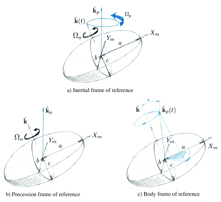
Figure 1: Schematic representation of the precessing ellipsoidal cavity. a) As seen from the frame of inertia, b) as seen from the frame of precession and c) as seen from the body frame

In figure 1, we represent the ellipsoidal cavity and the different vectors in the three frames of reference of interest for the present study. In the frame of inertia (fig. 1a), the precession vector is fixed, the cavity rotates around the time dependent vector $\hat{{\boldsymbol{k}}}(t)$, which describes a precessional motion around $\hat{{\boldsymbol{k}}}_{p}$. In the frame of precession (fig. 1b), both $\hat{{\boldsymbol{k}}}$ and $\hat{{\boldsymbol{k}}}_{p}$ are fixed and the cavity rotates around $\hat{{\boldsymbol{k}}}$ (the orientation of the principal axis of the cavity varies in time). In the body frame attached to the cavity (figure 1c), the orientation of the principal axes are fixed and the precession vector $\hat{{\boldsymbol{k}}}_{p}(t)$ exhibits a retrograde motion around $\hat{{\boldsymbol{k}}}$.

2.2 Coordinate systems

We define two systems of coordinates (figure 2): ($\hat{{\boldsymbol{X}}}_{m}$, $\hat{{\boldsymbol{Y}}}_{m}$, $\hat{{\boldsymbol{Z}}}_{m}$), attached to the ellipsoid and oriented along its principal axes $(a,b,c)$, and ($\hat{{\boldsymbol{X}}}_{p}$, $\hat{{\boldsymbol{Y}}}_{p}$, $\hat{{\boldsymbol{Z}}}_{p}$) that is attached to the precessing frame. In the rotating frame attached to the principal axes of the ellipsoid, the unit vectors $\hat{{\boldsymbol{X}}}_{p}$ and $\hat{{\boldsymbol{Y}}}_{p}$ rotate in a retrograde direction. We define the time origin such that at $t=0$, $\hat{{\boldsymbol{X}}}_{p}=\hat{{\boldsymbol{X}}}_{m}$, $\hat{{\boldsymbol{Y}}}_{p}=\hat{{\boldsymbol{Y}}}_{m}$. As shown on figure 2, $\hat{{\boldsymbol{Z}}}_{p}=\hat{{\boldsymbol{Z}}}_{m}$ at all times.

If we consider an arbitrary vector ${\boldsymbol{A}}$ of coordinates ($x_{p}$, $y_{p}$, $z_{p}$) in the coordinates system attached to the precessing frame, its coordinates in the system ($\hat{{\boldsymbol{X}}}_{m}$, $\hat{{\boldsymbol{Y}}}_{m}$, $\hat{{\boldsymbol{Z}}}_{m}$) are given by:

$$x_{m} = x_{p}\cdot\cos(\Omega_{o}t)+y_{p}\cdot\sin(\Omega_{o}t)$$

$$y_{m} = -x_{p}\cdot\sin(\Omega_{o}t)+y_{p}\cdot\cos(\Omega_{o}t)$$ (2)

$$z_{m} = z_{p}$$

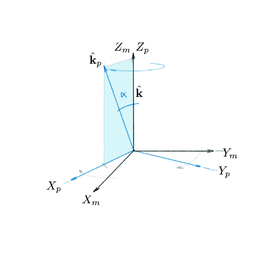
Figure 2: The coordinate systems: ($\hat{{\boldsymbol{X}}}_{m}$, $\hat{{\boldsymbol{Y}}}_{m}$, $\hat{{\boldsymbol{Z}}}_{m}$) is attached to the body and oriented along the principal axis (a,b,c) of the ellipsoid. In contrast, ($\hat{{\boldsymbol{X}}}_{p}$, $\hat{{\boldsymbol{Y}}}_{p}$, $\hat{{\boldsymbol{Z}}}_{p}$) is attached to the precessing frame.

In the frame of reference attached to the moving body, the equation of the triaxial ellipsoid boundary is given by:

$$\frac{x^{2}}{a^{2}}+\frac{y^{2}}{b^{2}}+\frac{z^{2}}{c^{2}}=1$$ (3)

In the present study, we will mostly consider two type of geometries, an axisymmetric spheroid ($a=b\neq c$), to which we refer as a spheroid, and a biaxial ellipsoid ($a\neq b=c$) to which we refer as the non axisymmetric ellipsoid. The true ellipsoidal geometry ($a\neq b\neq c$) will be referred to as the triaxial ellipsoid but will only be considered to derive the general inviscid equations, the fundamental dynamics due to a non axisymmetric equator being already captured when ($a\neq b=c$). The reduced tensor of inertia expressed in the coordinate system attached to the principal axes of the cavity reads

$$I=\frac{4\pi}{15}\left[\begin{array}[]{ccc}b^{2}+c^{2}&0&0\\ 0&a^{2}+c^{2}&0\\ 0&0&b^{2}+a^{2}\\ \end{array}\right].$$ (7)

2.3 Fluid equations of motion

Without further assumptions, the fluid motion inside the precessing ellipsoid is governed by the non-linear Navier-Stokes equation. Using $\Omega_{o}^{-1}$ as a time scale and $R=(abc)^{1/3}$ as a length scale, any velocity field ${\boldsymbol{u}}$ within the precessing ellipsoid is governed by the following equations, expressed in the body frame:

$$\frac{\partial{\boldsymbol{u}}}{\partial t}+2(\hat{\boldsymbol{k}}+Po\hat{{\boldsymbol{k}}}_{p})\times{\boldsymbol{u}}+{\boldsymbol{u}}\cdot\nabla{\boldsymbol{u}} = -\nabla p-Po(\hat{{\boldsymbol{k}}}_{p}\times\hat{{\boldsymbol{k}}})\times{\boldsymbol{r}}+E\,\Delta{\boldsymbol{u}},$$ (8)

$$\nabla\cdot{\boldsymbol{u}} = 0,$$ (9)

where $p$ is the reduced pressure which takes the centrifugal force into account, $Po=\Omega_{p}/\Omega_{o}$ is the so-called Poincaré number, and $E=\nu/(\Omega_{o}R^{2})$ is the Ekman number which represents the relative amplitude of the viscous and Coriolis forces.

If the fluid is viscous, the boundary condition is

$${\boldsymbol{u}}={\boldsymbol{0}},$$ (10)

which reduces to

$${\boldsymbol{u}}\cdot{\boldsymbol{n}}=0$$ (11)

for an inviscid fluid ($E=0$), with ${\boldsymbol{n}}$ the unit vector normal to the boundary surface.

Finally, we introduce the Rossby number that combines the rate of precession $Po$ and the angle of precession $\alpha$, it is a measure of the amplitude of the forcing:

$$Ro=Po||\hat{\boldsymbol{k}}_{p}\times\hat{\boldsymbol{k}}||=Po\sin\alpha$$ (12)

In former studies, the angle of precession $\alpha$ was fixed and the Poincaré number was varied, so does the Rossby number. In this study, we fix the Rossby number, $Ro=10^{-2}$, to ensure that the flow remains stable in our simulations, even at the largest values of $Po$. Consequently, the angle of precession varies as $\sin\alpha=Ro/Po$ as we scan in $Po$. It follows that there is a forbidden band $-10^{-2}<Po<10^{-2}$ for which no $\alpha$ can satisfy (12). The same study could be carried out at fixed $\alpha$ by varying the Poincar number the same conclusions would apply as long as no instability develop in the system. This means that there would be a forbidden zone depending on the critical values of Po, which we do not know. Note finally that to access the small Po region of the parameter space, one could simply reduce accordingly Ro.

2.4 Inviscid flows of uniform vorticity in triaxial precessing ellipsoids

Following the precursory work of Hough (1895), Sloudsky (1895) and Poincaré (1910) we assume the fluid to be inviscid and search for a solution of the velocity that is linear in the spatial coordinates $(x,y,z)$, i.e. a particular solution ${\boldsymbol{U}}$ of uniform vorticity

$${\boldsymbol{U}}={\boldsymbol{\omega}}\times{\boldsymbol{r}}+\nabla\psi,$$ (13)

where ${\boldsymbol{\omega}}$ is the mean rotation component of the flow and $\nabla\psi$ is the gradient flow needed to satisfy the non-penetration boundary condition. It is straightforward to show that such a solution does not generate any viscous force in the interior, which is consistent with our assumption.

Taking the curl of the Navier-Stokes equation (8) in the body frame, we obtain the vorticity equation for the particular flow (13):

$$\frac{\partial{\boldsymbol{\omega}}}{\partial t}=\left({\boldsymbol{\omega}}+Po\,\hat{{\boldsymbol{k}}}_{p}(t)+\hat{{\boldsymbol{k}}}\right)\cdot\nabla{\boldsymbol{U}}-Po\,\hat{{\boldsymbol{k}}}_{p}(t)\times\hat{{\boldsymbol{k}}},$$ (14)

An important step to establish the general equation for the mean vorticity is to express ${\boldsymbol{U}}$, or equivalently $\psi$, as a function of ($\omega,a,b,c,x,y,z$). This can be done by imposing the non-penetration condition on the velocity together with the condition of incompressibility, but this is rather lengthy. Instead, we propose to follow an approach similar to the original work of Poincaré (1910).

First, we introduce a geometrical transformation that applies in the body frame where the ellipsoid is fixed and that transforms the triaxial cavity $(a,b,c)$ into a sphere with a unit radius (fig. 3). Using a prime to denote quantities in the spherical domain and no prime for quantities in the true ellipsoid, we have:

$$x\rightarrow x^{\prime}=x/a,\,\,y\rightarrow y^{\prime}=y/b,\,\,z\rightarrow z^{\prime}=z/c.$$ (15)

The velocity is transformed following the same rules:

$$u_{x}\rightarrow u_{x}^{\prime}=u_{x}/a,\,\,u_{y}\rightarrow u_{y}^{\prime}=u_{y}/b,\,\,u_{z}\rightarrow u_{z}^{\prime}=u_{z}/c.$$ (16)

It is easy to show that the fluid in the spherical domain remains incompressible, of uniform vorticity, and does not penetrate the boundary. Note however, that it does not satisfy the ”no slip” nor the ”stress free” boundary conditions. Therefore it can only be a solution of the inviscid Euler equation (Tilgner, 1998). We now make use of this transformation and its reciprocal to easily obtain the analytical expression of the uniform vorticity flow in the body frame of the true ellipsoid.

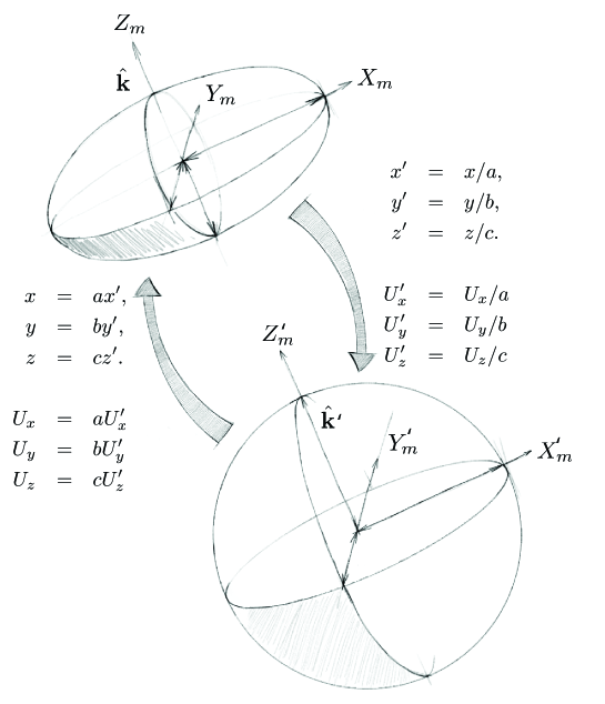
Figure 3: Schematic representation of the geometrical stretch that transforms a triaxial ellipsoid into a sphere of radius unity.

In the spherical domain, a flow of uniform vorticity simply takes the form of a solid body rotation:

$${\boldsymbol{U}}^{\prime}={\boldsymbol{\omega}}^{\prime}\times{\boldsymbol{r}}^{\prime}=(\omega^{\prime}_{y}z^{\prime}-\omega^{\prime}_{z}y^{\prime},\,\omega^{\prime}_{z}x^{\prime}-\omega^{\prime}_{x}z^{\prime},\,\omega^{\prime}_{x}y^{\prime}-\omega^{\prime}_{y}x^{\prime}).$$ (17)

Substituting (15-16) into (17) leads to

$${\boldsymbol{U}}=\left(\omega^{\prime}_{y}\frac{z}{c}-\omega^{\prime}_{z}\frac{y}{b},\,\omega^{\prime}_{z}\frac{x}{a}-\omega^{\prime}_{x}\frac{z}{c},\,\omega^{\prime}_{x}\frac{y}{b}-\omega^{\prime}_{y}\frac{x}{a}\right).$$ (18)

Since ${\boldsymbol{\omega}}^{\prime}$ is a uniform vector field, the mean vorticity in the ellipsoid is

$${\boldsymbol{\nabla}}\times{\boldsymbol{U}}=\left(\omega^{\prime}_{x}\left(\frac{c}{b}+\frac{b}{c}\right),\,\omega^{\prime}_{y}\left(\frac{a}{c}+\frac{c}{a}\right),\,\omega^{\prime}_{z}\left(\frac{b}{a}+\frac{a}{b}\right)\right)=2{\boldsymbol{\omega}}.$$ (19)

From (18) and (19), we finally obtain the analytical form of uniform vorticity inviscid flows in triaxial ellipsoids:

$$U_{x} = \omega_{y}\,\frac{2a^{2}}{a^{2}+c^{2}}\,z-\omega_{z}\,\frac{2a^{2}}{a^{2}+b^{2}}\,y,$$

$$U_{y} = \omega_{z}\,\frac{2b^{2}}{a^{2}+b^{2}}\,x-\omega_{x}\,\frac{2b^{2}}{c^{2}+b^{2}}\,z,$$ (20)

$$U_{z} = \omega_{x}\,\frac{2c^{2}}{b^{2}+c^{2}}\,y-\omega_{y}\,\frac{2c^{2}}{a^{2}+c^{2}}\,x.$$

Identifying the terms within (13), we obtain the expression for the potential field $\psi$:

$$\psi=\omega_{x}\,\frac{c^{2}-b^{2}}{c^{2}+b^{2}}\,yz+\omega_{y}\,\frac{a^{2}-c^{2}}{a^{2}+c^{2}}\,xz+\omega_{z}\,\frac{b^{2}-a^{2}}{b^{2}+a^{2}}\,xy.$$ (21)

Anticipating the rest of the paper we introduce, ${\boldsymbol{\Omega}}$, the space averaged rotation vector of the fluid in the precessing frame:

$${\boldsymbol{\Omega}}={\boldsymbol{\omega}}+\hat{{\boldsymbol{k}}}.$$ (22)

Using the coordinate system attached to the principal axes of the ellipsoid, we obtain from (2.2)

$$\omega_{x} = \Omega_{x}\cos(t)+\Omega_{y}\sin(t),$$

$$\omega_{y} = -\Omega_{x}\sin(t)+\Omega_{y}\cos(t),$$ (23)

$$\omega_{z} = \Omega_{z}-1.$$

Substituting the analytical expression of the velocity (2.4) in the vorticity equation (14), we obtain the general form of the equations that govern the inviscid solution of uniform vorticity in the body frame for a precessing triaxial ellipsoid:

$$\frac{\partial\omega_{x}}{\partial t}=2a^{2}\,\left[\frac{1}{a^{2}+c^{2}}-\frac{1}{a^{2}+b^{2}}\right]\omega_{z}\omega_{y}+P_{x}\sin(t)\frac{2a^{2}}{a^{2}+b^{2}}\omega_{z}$$ (24)

$$+\left(P_{z}+1\right)\frac{2a^{2}}{a^{2}+c^{2}}\omega_{y}+P_{x}\sin(t),$$ (25)

$$\frac{\partial\omega_{y}}{\partial t}=2b^{2}\,\left[\frac{1}{a^{2}+b^{2}}-\frac{1}{b^{2}+c^{2}}\right]\omega_{x}\omega_{z}+P_{x}\cos(t)\frac{2b^{2}}{a^{2}+b^{2}}\omega_{z}$$ (26)

$$-\left(P_{z}+1\right)\frac{2b^{2}}{b^{2}+c^{2}}\omega_{x}+P_{x}\cos(t),$$ (27)

$$\frac{\partial\omega_{z}}{\partial t}=2c^{2}\,\left[\frac{1}{b^{2}+c^{2}}-\frac{1}{a^{2}+c^{2}}\right]\omega_{x}\omega_{y}-P_{x}\cos(t)\frac{2c^{2}}{a^{2}+c^{2}}\omega_{y}$$ (28)

$$-P_{x}\sin(t)\frac{2c^{2}}{b^{2}+c^{2}}\omega_{x},$$ (29)

with $P_{x}=Po\sin\alpha=Ro$ and $P_{z}=Po\cos\alpha=Po\sqrt{Ro^{2}-Po^{2}}$. These equations are valid for any values of $(a,b,c)$, $Po$ and $\alpha$. In a spheroidal cavity there exist an infinite number of stationary solutions for the system (25-29) given by:

$${\boldsymbol{\omega}}+\hat{\boldsymbol{k}}=\xi\hat{\boldsymbol{k}}_{p},$$ (30)

where $\xi$ can be any real number. Among this class of inviscid solutions, only the solution $\xi=-Po$ remains stationary when $a\neq b$, for all $c$.

2.5 Reintroducing the viscosity

Without viscous damping, the inviscid solutions depend on the initial conditions and are somewhat of limited interest. Assuming the Ekman number to be small, we reintroduce the viscosity through the viscous torque due to the friction in the Ekman boundary layer.

In appendix A, we extend the approach of Noir et al. (2003) for a spheroid to the case of finite ellipticity. Without any loss of generality, the viscous equations (25-29) can be written as

$$\frac{\partial\omega_{x}}{\partial t}=\left[\frac{2a^{2}}{a^{2}+c^{2}}-\frac{2a^{2}}{a^{2}+b^{2}}\right]\omega_{z}\omega_{y}+P_{x}\sin(t)\frac{2a^{2}}{a^{2}+b^{2}}\omega_{z}$$ (31)

$$+\left(P_{z}+1\right)\frac{2a^{2}}{a^{2}+c^{2}}\omega_{y}+P_{x}\sin(t)+\left.\mathcal{L}{\boldsymbol{\Gamma}}_{\nu}\right|_{x},$$ (32)

$$\frac{\partial\omega_{y}}{\partial t}=\left[\frac{2b^{2}}{a^{2}+b^{2}}-\frac{2b^{2}}{b^{2}+c^{2}}\right]\omega_{x}\omega_{z}+P_{x}\cos(t)\frac{2b^{2}}{a^{2}+b^{2}}\omega_{z}$$ (33)

$$-\left(P_{z}+1\right)\frac{2b^{2}}{b^{2}+c^{2}}\omega_{x}+P_{x}\cos(t)+\left.\mathcal{L}{\boldsymbol{\Gamma}}_{\nu}\right|_{y},$$ (34)

$$\frac{\partial\omega_{z}}{\partial t}=\left[\frac{2c^{2}}{b^{2}+c^{2}}-\frac{2c^{2}}{a^{2}+c^{2}}\right]\omega_{x}\omega_{y}-P_{x}\cos(t)\frac{2c^{2}}{a^{2}+c^{2}}\omega_{y}$$ (35)

$$-P_{x}\sin(t)\frac{2c^{2}}{b^{2}+c^{2}}\omega_{x}+\left.\mathcal{L}{\boldsymbol{\Gamma}}_{\nu}\right|_{z}.$$ (36)

Using the linear asymptotic of spin-up and of the spin-over mode, we derive an analytical expression of the viscous term in the limit of small Ekman number.

$$\mathcal{L}{\boldsymbol{\Gamma}}_{\nu}=\sqrt{E\Omega}\left[\frac{\lambda^{r}_{so}}{\Omega^{2}}\left(\begin{array}[]{c}\Omega_{x}\Omega_{z}\\ \Omega_{y}\Omega_{z}\\ \Omega_{z}^{2}-\Omega^{2}\\ \end{array}\right)+\frac{\lambda^{i}_{so}}{\Omega}\left(\begin{array}[]{c}\Omega_{y}\\ -\Omega_{x}\\ 0\\ \end{array}\right)+\lambda_{sup}\frac{\Omega^{2}-\Omega_{z}}{\Omega^{2}}\left(\begin{array}[]{c}\Omega_{x}\\ \Omega_{y}\\ \Omega_{z}\\ \end{array}\right)\right],$$ (46)

where $\lambda_{so}^{r}$ and $\lambda_{so}^{i}$ represents the decay rate and viscous correction to the eigenfrequency of the spin-over mode, respectively. In the context of spheroids of finite ellipticity, we use the asymptotic values derived by Zhang et al. (2004). $\lambda_{sup}$ is an integrated value of the spin-up decay rate and is derived from the asymptotic theory of Greenspan (1968). We refer to this form of the viscous term as the generalized model in the rest of the paper

In the case of a non-axisymmetric container, no analytical solution for the inertial modes exists. In the lack of a proper theory for the viscous damping of inertial modes in a non axisymmetric container, we adopt the following reduced form for the viscous torque

$$\mathcal{L}{\boldsymbol{\Gamma}}_{\nu}=\lambda\sqrt{E}\left(\begin{array}[]{c}\Omega_{x}\\ \Omega_{y}\\ \Omega_{z}-1\\ \end{array}\right).$$ (50)

In appendix A.2, we show that, for an axisymmetric container, the viscous term (46) is well approximated by the reduced form (50) in the range of parameters considered in this study. Hence, $\lambda$ can be interpreted as an approximation of the decay rate $\lambda^{r}_{so}$ of the spin-over mode when the contribution from the terms proportional to $\lambda^{i}_{so}$ and $\lambda_{sup}$ are negligible. In the absence of model of the spin-over mode in a non-axisymmetric ellipsoid, $\lambda$ in our model remains an adjustable parameter and is determined so as to best fit the numerical results in each geometry. Herein, we refer to the viscous set of equation using (50) as the reduced model.

Anticipating the rest of the paper, we introduce the reduced viscous equations in the frame of precession for the particular class of ellipsoid ($a\neq b=c$). Substituting (2.2) into the inviscid set of equations (32-36) with $b=c$, we obtain:

$$\frac{\partial\Omega_{x}}{\partial t}=P_{z}\Omega_{y} + (1-\chi)\left[\cos(2t)\left(\frac{P_{z}+2}{2}\Omega_{y}-\frac{1}{2}\Omega_{y}\Omega_{z}\right)\right.$$ (51)

$$+ \sin(2t)\left(-\frac{P_{z}+2}{2}\Omega_{x}+P_{x}\Omega_{z}+\frac{1}{2}\Omega_{x}\Omega_{z}-P_{x}\right)$$

$$+ \left.\frac{P_{z}}{2}\Omega_{y}+\frac{1}{2}\Omega_{y}\Omega_{z}\right]+\lambda\sqrt{E}\Omega_{x},$$

$$\frac{\partial\Omega_{y}}{\partial t}=P_{x}\Omega_{z}-P_{z}\Omega_{x} + (1-\chi)\left[\cos(2t)\left(\frac{P_{z}+2}{2}\Omega_{x}-\frac{1}{2}\Omega_{x}\Omega_{z}-P_{x}\Omega_{z}+P_{x}\right)\right.$$ (52)

$$+ \sin(2t)\left(\frac{P_{z}+2}{2}\Omega_{y}-\frac{1}{2}\Omega_{y}\Omega_{z}\right)$$

$$- \left.\frac{P_{z}}{2}\Omega_{x}-\frac{1}{2}\Omega_{x}\Omega_{z}\right]+\lambda\sqrt{E}\Omega_{y},$$

$$\frac{\partial\Omega_{z}}{\partial t}=-P_{x}\Omega_{y} + (1-\chi)\left[\cos(2t)\left(\frac{P_{x}}{2}\Omega_{y}+\Omega_{x}\Omega_{y}\right)\right.$$ (53)

$$+ \sin(2t)\left(-\frac{P_{x}}{2}\Omega_{x}+\frac{1}{2}\left(\Omega_{y}^{2}-\Omega_{x}^{2}\right)\right)+\left.\frac{P_{x}}{2}\Omega_{y}\right]$$

$$+ \lambda\sqrt{E}(\Omega_{z}-1),$$

with the ratio $\chi$ of the two equatorial moments of inertia:

$$\chi=\frac{b^{2}+c^{2}}{a^{2}+b^{2}}=\frac{2b^{2}}{a^{2}+b^{2}}.$$ (54)

3 Comparison of the theoretical models with numerical simulations

To allow for an easy comparison with former studies we will focus our diagnostic on two quantities, the rotation vector of the fluid viewed from the frame of precession, $(\Omega_{x},\Omega_{y},\Omega_{z})$, and the amplitude of the differential angular velocity between the fluid and the surrounding container, $\|{\boldsymbol{\Omega}}-\hat{\boldsymbol{k}}\|$

3.1 Methods

The system of ordinary differential equations describing the time evolution of the uniform vorticity components of the flow, i.e. equations (32-36), is solved using the Dormand-Prince method, the standard version of the Runge-Kutta algorithm implemented in MATLAB. We have checked that the time evolution is not modified by the use of other time-stepping solvers.

The system of partial differential equations of the initial viscous problem, i.e the equations of motion (8-9) completed by the boundary condition (10) at the ellipsoid surface, is solved using a finite element method implemented in the commercial code COMSOL Multiphysics. The mesh element type used for the fluid variables is the standard Lagrange element $P1-P2$, which is linear for the pressure field and quadratic for the velocity field. For time-stepping, we use the Implicit Differential-Algebraic solver (IDA solver), based on variable-coefficient Backward Differencing Formulas or BDF (see Hindmarsh et al., 2005, for details on the IDA solver). The integration method in IDA is variable-order, the order ranging between 1 and 5. At each time step the system is solved with the sparse direct linear solver PARDISO (www.pardiso-project.org). All computations have been performed on a single workstation.

Since we are concerned with the effect of topography in our system, we have chosen to fix the Ekman number, $E=10^{-3}$, which allow us to use meshes with typically $30\,000$ degrees of freedom. Convergence tests in a spherical geometry have been performed to ensure that our simulations with this resolution capture correctly the viscous effects due the Ekman boundary layer. Figure 4 represents the norm of differential rotation between the fluid and the container in a spherical geometry, $\|{\boldsymbol{\Omega}}-\hat{\boldsymbol{k}}\|$. The red symbols represents the numerical simulations, the red dashed line represents the asymptotic solution of Busse (1968), the dashed blue line represents the generalized model (93- 95) and the green dashed line represents the reduced model. The best fit leads to $\lambda=-2.62$. We observe a quantitative agreement between all the models and the numerical simulations. A close look at the critical Po shows that the reduced model predicts a resonance at zero while the generalised model and Busse’s theory predicts a resonance at $Po\sim-0.01$. This difference is consistent with the fact that the reduced model does not account for the viscous correction of the eigenfrequency of the Poincar mode, which at these parameters is of order $0.01$.

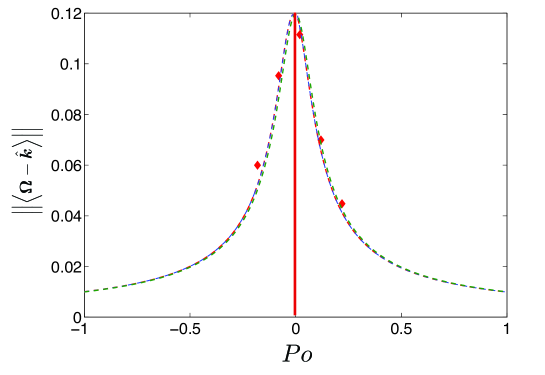
Figure 4: Equatorial component of the fluid mean rotation as a function of the Poincaré number in a spherical geometry. The numerical simulation are performed with $E=10^{-3}$ and $Ro=10^{-2}$. The red symbols represents the simulations, the red dashed line represents the asymptotic solution of Busse (1968), the blue dashed line represents the solution of generalized model (93-95) and the dashed green line represents the reduced model (32-36) with a derived value of $\lambda=-2.62$. The red vertical line symbolized the region of the parameter space $\left|Po\right|<10^{-2}$ where no $\alpha$ can satisfy $Ro=Po\sin(\alpha)$

In the present study we are concerned with the flow component of uniform vorticity. In the simulations, the uniform vorticity is obtained by averaging the fluid vorticity at each time step over a volume inside an ellipsoid:

$$\frac{x^{2}}{a^{2}}+\frac{y^{2}}{b^{2}}+\frac{z^{2}}{c^{2}}=d^{2},$$ (55)

with $d=1-5\sqrt{E}$ to exclude the Ekman boundary layer (see also Cébron et al., 2010b).

3.2 The axisymmetric spheroid, $a=b\neq c$

In this particular geometry, the reduced model systematically leads to a flow steady in the precessing frame.

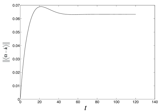
Figure 5: Time evolution of the amplitude of the equatorial component of rotation of the fluid in the frame of precession from the simulations. $a=b=1$, $c=0.5$, $E=10^{-3}$, $Ro=10^{-2}$ and $Po=-0.45$.

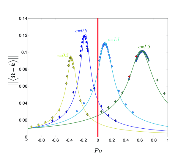
Figure 6: Amplitude of differential rotation, $\|{\boldsymbol{\Omega}}-\hat{\boldsymbol{k}}\|$, as a function of the Poincaré number. The symbols represent our numerical simulations simulations at $E=10^{-3}$ and $Ro=10^{-2}$, the solid lines represents the reduced model with the inverted values of $\lambda$ from table 1. Each value of the polar axis c is represented by a different color as indicated. The red vertical line signifies the region of the parameter space $\left|Po\right|<10^{-2}$ where no $\alpha$ can satisfy $Ro=Po\sin(\alpha)$. The red circles represent simulations with c=1.5 with a spatial resolution four times larger ($135000$ DoF).

Figure 5 represents the time evolution of the norm of the differential rotation, $\|{\boldsymbol{\Omega}}-\hat{\boldsymbol{k}}\|$ from the three-dimensional (3D) non linear simulations ($a=b=1$, $c=0.5$, $E=10^{-3}$, $Ro=10^{-2}$ and $Po=-0.45$). It shows that the uniform vorticity component becomes stationary after a typical period of $60$ rotations, which is comparable to the spin-up time $t\propto E^{-1/2}\sim 30$. This result is generic to all of our simulations in an axisymmetric spheroid. Hence, it validates the otherwise assumed stationarity of the uniform vorticity solution in the asymptotic theory of Busse (1968) and Noir et al. (2003).

Figure 6 shows the differential rotation, $\|{\boldsymbol{\Omega}}-\hat{\boldsymbol{k}}\|$ for $a=b=1$ and $c=0.5/0.8/1.1/1.5$ as we scan in Poincaré numbers from $-1$ to $+1$. For each geometry, we perform a least squares inversion using the reduced model to determine the value of $\lambda$ that best fits the numerical simulations. The results for each value of $c$ are presented in table 1. We choose to study each individual component in the precessing frame where the total vorticity remains time independent. Figure 7 shows the individual components of ${\boldsymbol{\Omega}}$ viewed from the precessing frame.

We retrieve the classical result that the amplitude of the differential rotation, $\|{\boldsymbol{\Omega}}-\hat{\boldsymbol{k}}\|$, exhibits resonant like peaks for a critical value of the Poincaré number, $Po_{c}$. Considering each individual component (Figure 7), the peaks correspond to a maximum of $\Omega_{y}$ and a (usually abrupt) change of sign of $\Omega_{x}$. As we shall see later at lower Ekman number, the term resonance may have a significance in the inviscid limit but for finite viscosity we prefer to use the term transition and define $Po_{c}$ as $\Omega_{x}(Po_{c})=0$, the transition thus corresponding to the abrupt change of direction of the mean rotation axis of the fluid. Physically, $Po_{c}$ is the Poincaré number for which the equatorial component of the fluid rotation is exactly aligned with the gyroscopic forcing $\hat{\boldsymbol{k}}_{p}\times\hat{\boldsymbol{k}}$, leading to a pseudo-resonance between the precessional forcing and the so-called Poincaré mode (see Noir et al. (2003) for more details). As expected from the asymptotic and inviscid theory, $Po_{c}<0$ for an oblate spheroid, $a>c$, and $Po_{c}>0$ for a prolate spheroid, $a<c$.

Figures 7 shows the components of ${\boldsymbol{\Omega}}$ (viewed from the frame of precession). We compare the three different models, Busse (1968), the generalized model and the reduced model to the numerical simulations. Comparing the relative amplitude of the different components, the differential motion is clearly dominated by the equatorial component, which thus governs the evolution of $\|{\boldsymbol{\Omega}}-\hat{\boldsymbol{k}}\|$ shown in figure 6. We observe a quantitative agreement between the reduced model and the numerical results for $\Omega_{x}$ and $\Omega_{y}$. The small departure of $\Omega_{z}$ from $1$ is less accurately captured by the model, owing to its weak influence on $\|{\boldsymbol{\Omega}}-\hat{\boldsymbol{k}}\|$ from which we invert for the unique adjustable parameter $\lambda$. Meanwhile, the generalized model, without any adjustable parameter, predicts correctly the resonance positions but tends to overestimate the amplitudes as $c$ is increased. One can however notice that the results of this predictive model are still acceptable for $c\in[0.5;1.1]$. In contrast, the usual Busse (1968) model does not predict correctly the flow components’ evolution, or even the resonance locations, as soon as the spheroid deformation becomes significant, which is expected given the domain of validity of this model.

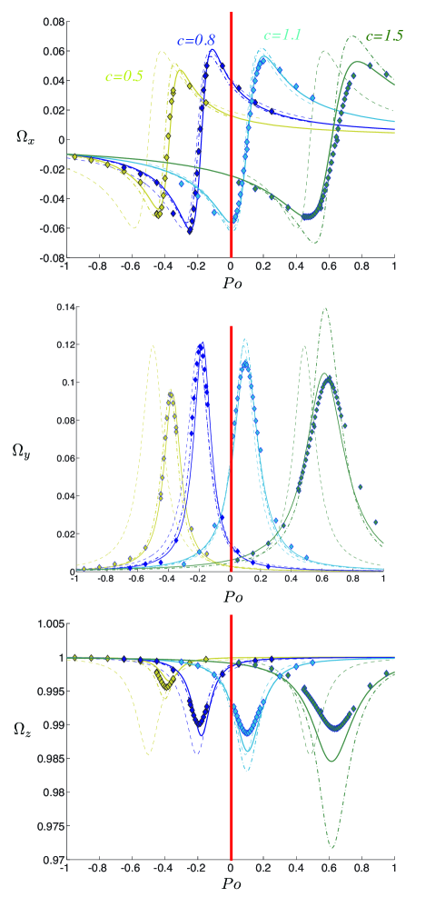
Figure 7: From top to bottom: X,Y and Z components of the fluid rotation vector in the frame of precession within an axisymmetric spheroid. We compare our simulations (symbols), the theory of Busse (1968), represented by the dashed lines, our generalization of this model (dot-dashed lines), and the proposed reduced model (solid lines) with the inverted values of $\lambda$ from table 1. Each value of the polar axis c is represented by a different color as indicated. The red vertical line symbolized the region of the parameter space $\left|Po\right|<10^{-2}$ where no $\alpha$ can satisfy $Ro=Po\sin(\alpha)$.

Table 1: Inverted viscous coefficient $\lambda$ for an axisymmetric spheroid

c	0.5	0.8	1.1	1.5
$\lambda$	-3.35	-2.57	-2.78	-2.97

3.2.1 The non-axisymmetric spheroid, $a\neq b=c=1$

Figure 8 represents the time evolution of the three components of the fluid rotation vector in the frame of precession from the 3D non linear numerical simulations with $a=0.5,\,b=c=1$. Comparison with figure 5 shows clearly an important difference: in non-axisymmetric ellipsoids, an unsteady and periodic flow can be forced by the precession contrary to the flow forced in a spheroid which is steady. The inset shows moreover that $\Omega_{x}$ and $\Omega_{y}$ oscillate in phase quadrature, with the same amplitude $\delta/2$ and the same period, which is half the container rotation period $T_{0}$ (dimensionless value of $T_{0}$ is $2\pi$).

Figure 9 represents the same data set as in Figure 8 plotted in three dimensions to illustrate the dynamics of the mean rotation vector. The fluid rotation vector performs a time periodic quasi circular motion (red dots) around its mean position (blue arrow). The semi-aperture angle of the cone is given by $\sqrt{\Omega_{x}^{2}+\Omega_{y}^{2}}$.

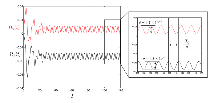
Figure 8: Time evolution of the three component of the fluid rotation vector in the frame of precession $\Omega_{x}(t)$, $\Omega_{y}(t)$ from the numerical simulations for $a=0.5,\,b=c=1$, $E=10^{-3}$, $Ro=10^{-2}$ and $Po=-0.45$.

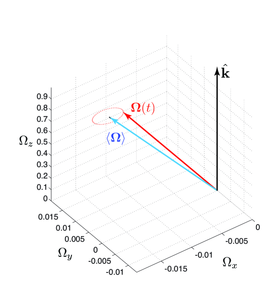
Figure 9: Time evolution of the fluid rotation vector ${\boldsymbol{\Omega}}$ viewed from the frame of precession (Same set of parameters as in Figure 8). The blue arrow represents the mean rotation vector $\left<{\boldsymbol{\Omega}}\right>$, the red arrow represents the instantaneous rotation vector at a particular time, the red dots show the trace of the instantaneous rotation vector for $60<t<120$ and the black arrow shows the container rotation vector.

We carry out a series of 3D numerical simulations for various geometries with $a\neq b=c$, in each case we perform the least squares inversion to determine $\lambda$ using only the time averaged differential rotation, $\|<{\boldsymbol{\Omega}}-\hat{\boldsymbol{k}}>\|$ (Figure 10). As in the case of an axisymmetric container, we observe peaks at critical values of the Poincaré number, identical in the mean and oscillatory components. We note that the critical $Po$ is retrograde for $a>1$ and prograde for $a<1$, which correlates with the results obtained in an axisymmetric spheroid. Indeed, in any meridional cross section of the non axisymmetric cavity, the trace of the boundary is an ellipse with a polar axis shorter than the mean equatorial axis for $a>1$, similarl to an oblate spheroid, and longer than the mean equatorial axis for $a<1$, similarl to a prolate spheroid. As the geometry tends toward the sphere $(a=1)$, the amplitude of the peak of the oscillatory component vanishes, while the peak of the time averaged component converges toward the solution for the sphere as illustrated in Figure 10.

We observe a quantitative agreement between our reduced model and the numerical simulations for both the mean and oscillatory components for all cases with $a>b=c$. For $a<b=c$, the reduced model captures correctly the dynamics of the time average equatorial rotation but exhibit significant discrepancy in the axial components.

Table 2: Inverted viscous coefficient $\lambda$ for an non axisymmetric spheroid

a	0.5	1.1	1.5	2
$\lambda$	$-4.5\pm 0.02$	$-2.54\pm 0.02$	$-2.29\pm 0.02$	$-2.03\pm 0.02$

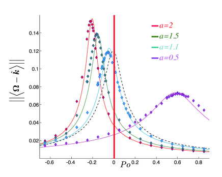
Figure 10: Amplitude of the mean differential rotation, $\|<{\boldsymbol{\Omega}}-\hat{\boldsymbol{k}}>\|$, as a function of the Poincaré number. The symbols represent numerical simulations at $E=10^{-3}$ and $Ro=10^{-2}$, the solid lines represent the inverted reduced model, the black-dashed line represents the solution for the sphere from Busse (1968). Each geometry, characterized by $a$, is represented with a different color as indicated. The red vertical line symbolized the region of the parameter space $\left|Po\right|<10^{-2}$ where no $\alpha$ can satisfy $Ro=Po\sin(\alpha)$.

Figure 11 shows the time averaged and oscillatory components, respectively, of ${\boldsymbol{\Omega}}$. The steady part of the uniform vorticity behaves as in an axisymmetric container, its axial component $\Omega_{z}$ departs only marginally from the vorticity of the container, hence, the differential motion between the fluid and the container is dominated by the equatorial component. Even though we invert for the unique adjustable parameter using the steady part only, we observe a very good agreement between the reduced model and the simulations. All three components exhibit a maximum amplitude at the critical $Po_{c}$ derived from the time average part. As suggested from the time evolution shown in Figure 8, the two equatorial components have the same amplitude, the axial component is only five times smaller. In addition, we note a significant discrepancy both on the peak location and amplitude between the reduced model and the numerical simulations for $a=0.5$, similarly to the case of a prolate axisymmetric spheroid.

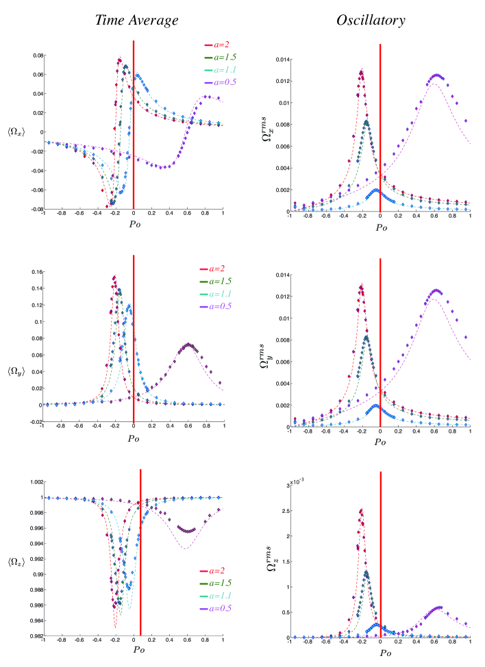
Figure 11: From top to bottom: X,Y,Z-component of rotation of the fluid in the frame of precession. The left row shows the time averaged components, the right row shows the time standard deviation of the components. We compare, for each geometry (i.e. $a$), our simulations (symbols) and the reduced model (dashed lines) with the inverted values of $\lambda$ from table 2. The red vertical line is the region of the parameter space $\left|Po\right|<10^{-2}$ where no $\alpha$ can satisfy $Ro=Po\sin(\alpha)$.

4 Discussion

In appendix A.2, we show that the location of the $Po_{c}$, within an axisymmetric container, is determined primarily by the inviscid part of the equations, while the typical amplitude is most constrained by the decay rate $\lambda_{so}^{r}$. We also note that the viscous correction to the spin-over eigenfrequency accounts for a small shift of $Po_{c}$ but does not modify the fundamental dynamics, even at the moderate Ekman numbers considered here. Finally, the effect of the non vanishing axial differential rotation in the frame rotating with the fluid remains negligible in all of our simulation. The systematic mismatch of the amplitude of the generalized model with our simulations is likely due to the moderate Ekman numbers accessible in our numerical simulations. Meanwhile, the observed shift in $Po_{c}$ in Figure 7 and Figure 11 shows the limitations of the one adjustable parameter reduced model that only account for part of the dissipation mechanism.

The simulations presented here show that the flow of uniform vorticity in a non axisymmetric ellipsoid is not purely stationary in the frame of precession as it would be for a spheroidal cavity. This is supported by the governing equations (51-53) from which one can anticipate that, if a stationary uniform vorticity component exists, it will necessarily drive a time dependent perturbation for $\chi\neq 1$, i.e. when the two equatorial moments of inertia are not equal.

Our results suggest that the simple form of the viscous term (50) captures well the fundamental dynamics of the uniform vorticity flow in a non axisymmetric precessing ellipsoid. Taking advantage of the computational efficiency of this reduced model, we perform a series of time integrations at lower Ekman numbers. Figure 12 shows the norm of the mean and oscillatory components of the differential ${\boldsymbol{\Omega}}-\hat{\boldsymbol{k}}$ as a function of the Poincaré number for decreasing Ekman numbers in the case $a=1.5,\,b=c=1$; we assume the decay rate $\lambda$ to be independent of the Ekman number and equal to the value inverted in this geometry at $E=10^{-3}$ (see table 2). As the Ekman number is reduced, both the stationary and the oscillatory part of the differential rotation tend toward an asymptotic limit already captured at $10^{-7}$.

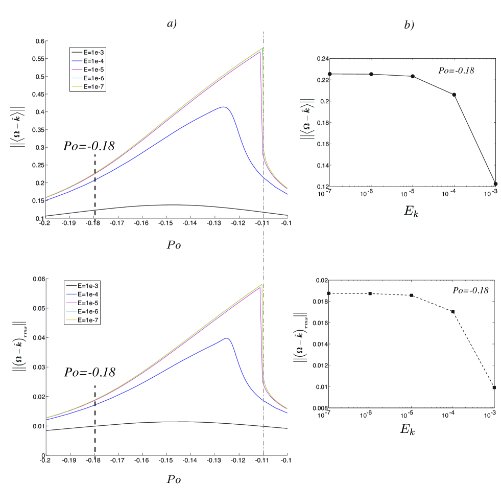
Figure 12: a) Upper panel: norm of the stationary component of the differential rotation ${\boldsymbol{\omega}}$ as function of the Ekman number. Lower panel: norm of the oscillatory component of the differential rotation ${\boldsymbol{\omega}}$ as function of the Ekman number. b) Norm of the stationary (upper) and oscillatory (lower) part of the differential rotation for a fixed $Po=-0.18$ as a function of the Ekman number. In all calculations we integrate in time the reduced model with $a=1.5,\,b=c=1$ and $\lambda=-2.3$.

Let us define the mean longitude $\phi$ and the mean latitude $\theta$ of the fluid rotation axis as follows:

$$\cos\phi = \frac{\left<\Omega_{x}\right>}{\sqrt{\left<\Omega_{x}\right>^{2}+\left<\Omega_{y}\right>^{2}}},$$ (56)

$$\tan\theta = \frac{\left<\Omega_{z}\right>}{\sqrt{\left<\Omega_{x}\right>^{2}+\left<\Omega_{y}\right>^{2}}}.$$ (57)

Figure 13 shows the evolution of the longitude and latitude for decreasing Ekman numbers. As for the amplitude, we observe that the direction of the stationary component of uniform vorticity tends toward an asymptotic value. We note that the asymptotic longitude is either $0^{\circ}$ or $180^{\circ}$, which corresponds to a fluid mean rotation vector lying in the plane $(\hat{\boldsymbol{k}},\hat{\boldsymbol{k}}_{p})$. Hence, similarly to the case of an axisymmetric spheroid, it is the viscosity that forces the mean rotation vector to leave the plane containing the axis of the container and the axis of precession. In that plane, at vanishing Ekman numbers, the rotation vector evolves from high latitudes (${\boldsymbol{\Omega}}$ almost aligned with $\hat{\boldsymbol{k}}$), far from the transition, to mid latitudes near the transition.

Our results suggest that at low enough Ekman number, the flow of uniform vorticity driven by the precession of the container becomes independent of $E$, or as a matter of fact, independent of the viscous term $\lambda\sqrt{E}$. Hence, outside of the transition region, the asymptotic solution for vanishing viscosity can be found using any arbitrary order $\mathcal{O}(1)$ value of the damping factor, providing that the Ekman number is small enough, typically when $E^{1/2}\lesssim(1-\chi)$.

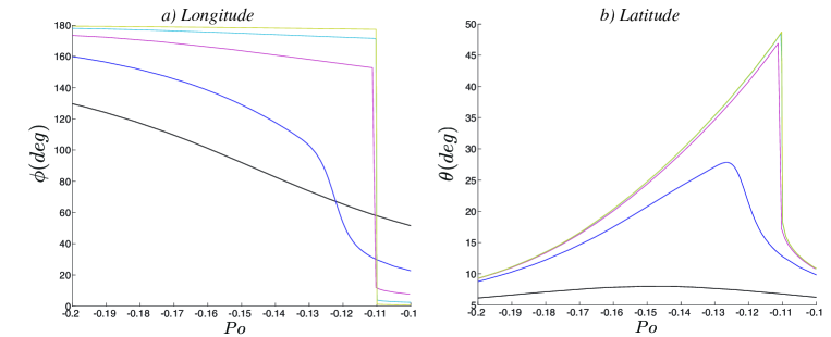
Figure 13: a) Longitude of the stationary part of the rotation vector. b) Latitude of the stationary part of the rotation vector. Color code: same as Figure 12.

5 Conclusion

In the present study, we investigate the flow of uniform vorticity driven by precession in a spheroid and a non axisymmetric ellipsoid. We report the first numerical simulations in a non axisymmetric ellipsoid showing that, in contrast to a spheroid, the flow of uniform vorticity viewed from the frame of precession is no longer stationary.

In addition, we develop a semi-analytical model by first deriving the inviscid equations and then by reintroducing the viscosity. We propose a generalized model in the case of a spheroid of arbitrary ellipticity following the torque approach introduced by Noir et al. (2003) and using the linear asymptotic theory of the spin-over mode as a proxy. For non axisymmetric ellipsoids an analoguous theory has yet to be established and the same approach is not possible. Nevertheless, we introduce a reduced model with one adjustable parameter that we compare successfully with 3D non-linear numerical simulation at a fixed Ekman number, $E=10^{-3}$ (using the commercial software Comsol).

Despite its simplicity, the reduced model with one adjustable parameter allows us to reproduce quantitatively the uniform vorticity flow obtained from numerical integrations of the full Navier-Stokes equations both in a spheroid and a non axisymmetric ellipsoid. Furthermore, the generalized model for a spheroid allow us to extend the classical asymptotic theory of Busse (1968); Noir et al. (2003) to finite ellipticity as it is usually the case in laboratory experiments. With our current limited number of geometrical configurations (4 different values of a) it is not possible to ascertain the functional relationship between the geometrical deformation and the damping factor.

Taking advantage of the computational efficiency of the reduced model compared to the full simulations of Navier-Stokes equations, we investigate the uniform vorticity flow in non axisymmetric ellipsoids as the Ekman number is decreased. We show that the uniform vorticity converges toward an asymptotic solution independent of the Ekman number and thus of the viscous term as a whole. At very low Ekman numbers, the time averaged component of the fluid rotation axis lies in the plane formed by the precession and container rotation vectors as in the case of a spheroid, meanwhile the time dependent component tends toward a finite amplitude.

Table 3: Dimensionless parameters for the Earth’s moon.

$1-\chi$	$2.5\times 10^{-5}$	Le Bars et al. (2011)
$E$	$\sim 10^{-12}$	Le Bars et al. (2011)
$Po$	$-3.9\times 10^{-3}$	Meyer & Wisdom (2011)
$\alpha$	$1.54$	Meyer & Wisdom (2011)

When looking at the dynamics in greater details we identify some limitations of our reduced model: first, there is a small shift of the critical value of the Poincaré number at which we observe a transition, and second the axial component of the fluid rotation exhibits a simpler dynamics in our reduced model than in the numerical simulations.

Due to the limited range of Ekman numbers accessible in the numerical simulations, we believe that an experimental survey is necessary to complement the results presented in this study. With an experimental setup using water as a working fluid, a typical length scale $\sqrt{abc}\sim 15$ cm and rotating at $\Omega_{0}\sim 240$ rpm, the achievable Ekman number will be of order $3\times 10^{-6}$. Aside from testing the validity of the reduced model, it would be suitable to investigate the stability of the flow.

Two recent publications have investigated possible mechanisms to drive Earth’s Moon early dynamo. One invokes a precession driven turbulence in the liquid core (Dwyer et al., 2011), whereas the other one proposes a meteoritic impact leading to a desynchronization of the Moon (Le Bars et al., 2011). Considering our current tidally-locked Moon, the core-mantle boundary (CMB) geometry is close to a non-axisymmetric ellipsoid rather than a axisymmetric spheroid (typically, its shape can be approximated by the well known relation $(b-c)/(a-c)=1/4$ assuming hydrostatic state and homogeneous material). We can thus compare our reduced model, assumed to be valid for our current Moon, and the model of Busse (1968), which is valid at planetary settings but assumes a spheroidal CMB. The parameters used for the simulation are given in table 3. The reduced model for a non axisymmetric ellipsoid and the model of Busse (1968) for a spheroid agree within $0.3\%$ leading to a mean differential rotation amplitude of order $3\%$ of the planet rotation rate and a core spin vector normal to the ecliptic plane in agreement with a former model by Goldreich (1967). Neither the viscous nor the pressure torques are large enough to force the lunar core to precess with the mantle. Nevertheless, in contrast with a spheroidal model, the reduced model predicts an unsteady component of uniform vorticity of order $2.3\times 10^{-6}\,\Omega_{o}$ oscillating with a period of $T\approx 13.5$ days. Although this amplitude is small, one may question what could happen if in the frame of precession there exists another source of gravitational perturbation at that frequency. Indeed, in that case, direct or parametric resonances may occur, leading to much larger amplitude flows, subsequent instabilities, and thus to enhanced dissipation.

Appendix A The viscous torque for a precessing spheroid of arbitrary ellipticity

A.1 The viscous torque

In the limit of small ellipticity, small Ekman number and small $Po\sin\alpha$, Busse (1968) and Noir et al. (2003) have derived the viscous equations for the stationary flow of uniform vorticity in a precessing axisymmetric spheroid. We herein refer to this model as Busse 1968, who was the first one to derive it in the limit of small ellipticity, small Ekman number and small $Po\sin(\alpha)$. In this appendix, we follow the same approach as Noir et al. (2003) to derive a more general model for finite ellipticity.

To reintroduce the viscosity, we assume a small Ekman number such that, at leading order, the uniform vorticity solution in the bulk remains essentially inviscid and the viscous forces are important only in the Ekman boundary layer. The Navier-Stokes equation for an arbitrary viscous flow ${\boldsymbol{u}}$ in the frame of precession leads to the following torque balance in the precessing frame (within the spheroid volume $V$):

$$\overbrace{\int_{V}\boldsymbol{r}\times\frac{\partial{\boldsymbol{u}}}{\partial t}\textrm{d}V}^{\boldsymbol{\Gamma_{t}}}+\overbrace{\int_{V}\boldsymbol{r}\times({\boldsymbol{u}}\cdot\nabla{\boldsymbol{u}})\textrm{d}V}^{\boldsymbol{\Gamma_{nl}}}+\overbrace{2\int_{V}\boldsymbol{r}\times(\boldsymbol{\Omega_{p}}\times{\boldsymbol{u}})\textrm{d}V}^{\boldsymbol{\Gamma_{i}}}=$$

$$\overbrace{-\int_{V}\boldsymbol{r}\times\nabla p\textrm{d}V}^{\boldsymbol{\Gamma_{p}}}+\overbrace{E\int_{V}\boldsymbol{r}\times\nabla^{2}{\boldsymbol{u}}\textrm{d}V}^{\boldsymbol{\Gamma_{v}}}.$$ (59)

The challenge is thus to obtain the viscous torque due to the Ekman layer.

As previously, we consider a uniform vorticity flow in a spheroid, which can be seen as a quasi solid body rotation along an axis tilted from the container rotation axis. Note that no further assumption is made on the stationarity in the frame of precession. For the particular flow ${\boldsymbol{U}}={\boldsymbol{\omega}}\times{\boldsymbol{r}}+{\boldsymbol{\nabla}}\phi$, the integration of ${\boldsymbol{\Gamma_{t}}}$, which is carried in the coordinates system attached to the ellipsoidal container, leads to:

$$\mathcal{L}{\boldsymbol{\Gamma}}_{t}=\frac{\partial{\boldsymbol{\omega}}}{\partial t},$$ (60)

where $\mathcal{L}$ is the matrix:

$$\mathcal{L}=\frac{15}{16\pi}\left[\begin{array}[]{ccc}\frac{b^{2}+c^{2}}{b^{2}c^{2}}&0&0\\ 0&\frac{a^{2}+c^{2}}{a^{2}c^{2}}&0\\ 0&0&\frac{b^{2}+a^{2}}{b^{2}a^{2}}\\ \end{array}\right].$$ (64)

The differential rotation between the fluid and the surrounding container in the frame can be decomposed into an axial and an equatorial component relative to the rotation axis of the fluid:

$${\boldsymbol{\delta\omega}}_{z} = \left(\frac{{\boldsymbol{\Omega}}-\hat{\boldsymbol{k}}}{\Omega^{2}}\cdot{\boldsymbol{\Omega}}\right){\boldsymbol{\Omega}},$$ (65)

$${\boldsymbol{\delta\omega}}_{eq} = {\boldsymbol{\Omega}}-\hat{\boldsymbol{k}}-{\boldsymbol{\delta\omega}}_{z}.$$ (66)

Without the viscous torque acting on the fluid, the equatorial component would tend to grow a spin-over mode, while the axial component would result in a spin-up or spin-down of the fluid. Thus, following the approach of Noir et al. (2003), the viscous torque can be derived from the linear decay rate of Greenspan for the spin-over and spin-up:

$$\mathcal{L}{\boldsymbol{\Gamma}}_{\nu}^{eq,z}=\left.\frac{\partial({\boldsymbol{\delta\omega}}_{eq,z})}{\partial t}\right|_{t=0}.$$ (67)

Since the linear calculation is only valid in the frame rotating with the fluid, we introduce a modified Ekman number $E_{f}=E/\Omega$ and a rescaled time $t_{f}=\Omega t$ associated to this frame of reference. According to Greenspan (1968), the time evolution of the spin-over mode in the non-rotating frame can be written as (Noir et al., 2003):

$${\boldsymbol{\delta\omega}}_{eq}(t)=\exp\left(\lambda^{r}_{so}E_{f}^{1/2}t_{f}\right) \left[{\boldsymbol{\delta\omega}}_{eq}(0)\,\cos\left(\lambda^{i}_{so}E_{f}^{1/2}t_{f}\right)\right.$$ (68)

$$-\left.{\boldsymbol{\Omega}}\times{\boldsymbol{\delta\omega}}_{eq}(0)\,\sin\left(\lambda^{i}_{so}E_{f}^{1/2}t_{f}\right)/\Omega\right].$$

It follows:

$$\mathcal{L}{\boldsymbol{\Gamma}}_{\nu}^{eq}=(E\Omega)^{1/2}\left[\frac{\lambda^{r}_{so}}{\Omega^{2}}\left(\begin{array}[]{ccc}\Omega_{x}\Omega_{z}\\ \Omega_{y}\Omega_{z}\\ \Omega_{z}^{2}-\Omega^{2}\\ \end{array}\right)+\frac{\lambda^{i}_{so}}{\Omega}\left(\begin{array}[]{ccc}\Omega_{y}\\ -\Omega_{x}\\ 0\\ \end{array}\right)\right].$$ (75)

In contrast with Noir et al. (2003), who use the $\lambda^{r}_{so},\,\,\lambda^{i}_{so}$ in the spherical approximation of Greenspan (1968), we propose to use the analytical prediction of $\lambda^{r}_{so},\,\,\lambda^{i}_{so}$ obtained from Zhang et al. (2004) in an oblate spheroid ($c<a$) of arbitrary ellipticity. Although the author does not claim that his derivation remains valid in a prolate spheroid ($c>a$), we have checked that the formula reproduces the results of Greenspan (1968) and are thus valid for prolate spheroids. It is important to note that the derivation of the spin-over decay rate are valid only for an axisymmetric container. Then, if the tilt of the fluid rotation axis and the ellipticity is not small enough, the viscous torque in the precessing cavity can no longer be inferred from the axisymmetric spin-over mode asymptotic theory introduced above.

The axial differential rotation can be treated similarly. Without the viscous torque the axial differential rotation would tend to spin-up or spin-down the fluid. From Greenspan (1968), the time evolution of an axial differential rotation can be written as

$${\boldsymbol{\delta\omega}}_{z}(s,t)={\boldsymbol{\delta\omega}}_{z}(0)\left(1-\exp(\lambda_{sup}^{*}(s)\,E_{f}t_{f})\right),$$ (76)

with a coefficient $\lambda_{sup}^{*}(s)$ which changes with the cylindrical radius $s$. An explicit analytical expression of $\lambda_{sup}^{*}(s)$ is given by Greenspan & Howard (1963) for axisymmetric containers, which can be written in the case of a spheroid as:

$$\lambda_{sup}^{*}(s)=-\frac{[1-s^{2}(1-c^{2})]^{1/4}}{c\,(1-r^{2})^{3/4}}.$$ (77)

Hence, the axial viscous torque can be estimated as:

$$\mathcal{L}{\boldsymbol{\Gamma}}_{\nu}^{z}=\lambda\sqrt{E}_{sup}\left(1-\frac{\Omega_{z}}{\Omega^{2}}\right)\left(\begin{array}[]{ccc}\Omega_{x}\\ \Omega_{y}\\ \Omega_{z}\\ \end{array}\right),$$ (81)

with

$$\lambda_{sup}=\int\lambda_{sup}^{*}(s)\,\textrm{d}s=-\frac{\sqrt{\pi^{3}/2}}{c\,\mathrm{\Gamma}(3/4)^{2}}\,\mathrm{F}\left([-1/4,1/2],[3/4],1-c^{2}\right),$$ (82)

where $\mathrm{\Gamma}$ is simply the gamma function and $\mathrm{F}(n,d,z)$ is the usual generalized hypergeometric function, also known as the Barnes extended hypergeometric function (see respectively chap. 6 and 15 of Abramowitz & Stegun, 1972). Note that when the tilt of the fluid mean rotation axis with the one of the mantle becomes large, i.e. when the container is no longer axisymmetric from the fluid point of view, we do not expect this derivation of the torque to apply either.

Finally, taking into account both the spin-up and spin-over contributions, it yields

$$\mathcal{L}{\boldsymbol{\Gamma}}_{\nu}=\sqrt{E\Omega}\left[\frac{\lambda^{r}_{so}}{\Omega^{2}}\left(\begin{array}[]{c}\Omega_{x}\Omega_{z}\\ \Omega_{y}\Omega_{z}\\ \Omega_{z}^{2}-\Omega^{2}\\ \end{array}\right)+\frac{\lambda^{i}_{so}}{\Omega}\left(\begin{array}[]{c}\Omega_{y}\\ -\Omega_{x}\\ 0\\ \end{array}\right)+\lambda_{sup}\frac{\Omega^{2}-\Omega_{z}}{\Omega^{2}}\left(\begin{array}[]{c}\Omega_{x}\\ \Omega_{y}\\ \Omega_{z}\\ \end{array}\right)\right].$$ (92)

Substituting (2.2) into the equations (32-36) with $a=b$, we obtain the viscous equations in the frame of precession:

$$\frac{\partial\Omega_{x}}{\partial t} = P_{z}\Omega_{y}-(1-\gamma)\left[P_{z}\Omega_{y}+\Omega_{y}\Omega_{z}\right]+\mathcal{L}{\boldsymbol{\Gamma}}_{\nu}\cdot\hat{\boldsymbol{e}}_{x},$$ (93)

$$\frac{\partial\Omega_{y}}{\partial t} = P_{x}\Omega_{z}-P_{z}\Omega_{x}+(1-\gamma)\left[P_{z}\Omega_{x}+\Omega_{x}\Omega_{z}\right]+\mathcal{L}{\boldsymbol{\Gamma}}_{\nu}\cdot\hat{\boldsymbol{e}}_{y},$$ (94)

$$\frac{\partial\Omega_{z}}{\partial t} = -P_{x}\Omega_{y}-(1-\gamma)P_{x}\Omega_{y}+\mathcal{L}{\boldsymbol{\Gamma}}_{\nu}\cdot\hat{\boldsymbol{e}}_{z},$$ (95)

where $\gamma=(2a^{2})/(a^{2}+c^{2})$ represents the ration of the polar to equatorial moment of inertia.

Taking (93)$\times\Omega_{x}+$ (94)$\times\Omega_{y}+$ (95)$\times\Omega_{z}$ yields,

$$({\boldsymbol{\Omega}}-\hat{\boldsymbol{k}})\cdot{\boldsymbol{\Omega}}=\frac{(1-\gamma)P_{x}\Omega_{y}\Omega_{z}}{\lambda_{sup}\sqrt{E}}.$$ (96)

Then, in the limit $(1-\gamma)P_{x}/\sqrt{E}\ll 1$, we recover the so called no spin-up condition introduced by Noir et al. (2003), also equivalent to the solvability condition of Busse (1968). This condition, also used by Cébron et al. (2010b), is thus not valid in general for a spheroid of arbitrary ellipticity.

A.2 Comparison between the different models in an axisymmetric spheroid.

Substituting (2.2) into the equations (32-36) with $a=b$, we obtain the viscous equations in the frame of precession. We thus have three different models for the axisymmetric spheroid: the asymptotic analysis of Busse (1968), our generalized model and our reduced model. The fundamental differences between all three models are twofold. First the model of Busse (1968); Noir et al. (2003) uses an approximate form of the inviscid part of the equations, valid only for small departure from the sphere ($1-\gamma\ll 1$) and for small $Po\ll 1$, while the generalized and reduced models uses an exact derivation for the inviscid part. Second all three models are based on a different derivation of the viscous torque: Busse (1968); Noir et al. (2003) are based on the asymptotic values of $\lambda_{so}^{i,r}$ of the sphere and on the no spin-up condition, the generalized model uses the asymptotic values of $\lambda_{so}^{i,r}$ for an oblate spheroid of arbitrary ellipticity from Zhang et al. (2004) and does not impose the no spin-up condition, and finally the reduced model neglects the terms proportional to $\lambda_{so}^{i}$ and $\lambda_{sup}$ and we thus have to close by fitting the best value of $\lambda_{so}^{r}$.

Figure 14(a) shows the contribution of the different terms of the viscous torque in the generalized model (75-81). We observe that throughout the entire range of $Po$ and for all geometries, the terms proportional to $\lambda_{sup}$ (due to the axial differential rotation) remains two to three orders of magnitude smaller than the term proportional to $\lambda^{r}_{so}$ and can therefore be neglected. The contribution from the term proportional to $\lambda^{i}_{so}$ remains four to twenty times smaller than the term proportional to $\lambda^{r}_{so}$. Although not negligible, this term is expected to have a limited effect on the dynamics of the uniform vorticity flow. In most of our simulations, the generalized model reduces thus to the reduced model. This is illustrated in Figure 14(b) which compares, for the axisymmetric spheroids considered in this study, the generalized and reduced models with the same value of $\lambda_{so}^{r}$. We observe a small shift in the peaks location which reflects the absence of the correction in $\lambda^{i}_{so}$ in the reduced model. In agreement with Figure 14(a), this shift is larger for $c=0.5$, where both the $\lambda_{so}^{r}$ and $\lambda_{so}^{i}$ contributions are of the same order.

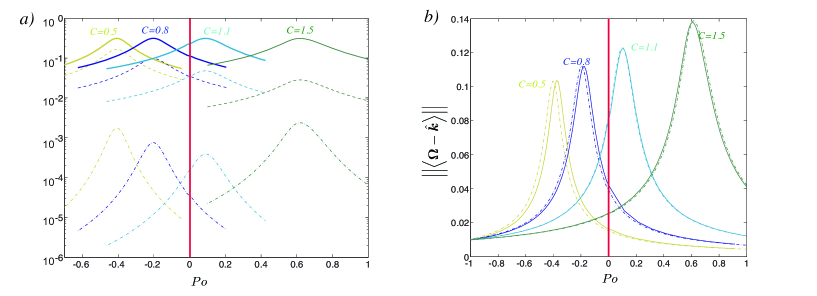
Figure 14: a) Amplitude of the viscous terms in the generalized model associated with $\lambda^{r},\,\lambda^{i}$ and $\lambda_{sup}$ (75-81). The color scheme stands for the different polar flattening as indicated, the solid line represents the contribution from the $\lambda^{r}$-term, the dashed line represents the contribution from the $\lambda^{i}_{so}$-term and the dot-dashed line represents the contribution from the $\lambda_{sup}$-term. b) Comparison of the equatorial component of rotation between the generalized model (dot-dashed lines) and the reduced model (solid lines). In both models we use, $a=b=1$, $c=0.5/0.8/1.1/1.5$, $E=10^{-3}$, $Ro=10^{-2}$ and the values of $\lambda^{r},\,\lambda^{i}$ of Zhang et al. (2004). The red vertical line symbolized the region of the parameter space $\left|Po\right|<10^{-2}$ where no $\alpha$ can satisfy $Ro=Po\sin(\alpha)$.

We now compare the generalized model and reduced models with $\lambda=\lambda_{so}^{r}=-3.03$ (Zhang et al., 2004) to the asymptotic solution of Busse (1968); Noir et al. (2003) using both the asymptotic value $\lambda=\lambda_{so}^{r}=-2.62$ (Greenspan, 1968) and the asymptotic value $\lambda=\lambda_{so}^{r}=-3.03$ (Zhang et al., 2004) (Figure 15). In addition, we represent the $Po_{c}$ for the classical inviscid of Poincaré obtained by substituting $\mathcal{L}\boldsymbol{\Gamma_{\nu}}=0$ in (93-95) and assuming a stationary solution. It illustrates that the location of the peak is determined primarily by the inviscid form of the equations, that are exact in our model and approximated for small $Po$ and small ellipticity in Busse (1968); Noir et al. (2003). Meanwhile, as seen from our reduced model, the variation in $\lambda^{i}_{so}$ contributes to a small detuning of the peak but the amplitude is mostly determined by the decay rate $\lambda^{r}_{so}$.

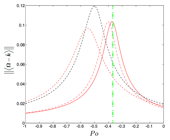
Figure 15: Norm of the differential rotation for $a=b=1$, $c=0.5$, $E=10^{-3}$, $Ro=10^{-2}$ The solid lines represents the reduced models, the dashed line represents the asymptotic theory of Busse (1968); Noir et al. (2003) and the dot-dashed line represents the generalized model. The color scheme stands for the different values of $\lambda_{so}^{r},i$, from Greenspan (1968) (black) and from Zhang et al. (2004) (red). The green dot-dashed line represents the critical Po predicted from a purely inviscid model.

This validates the use of the reduced model in the case of an axisymmetric spheroid and we are confident that the same general remarks apply to the case of a non axisymmetric container.

References

- Abramowitz & Stegun (1972) Abramowitz, M. & Stegun, I. 1972 Handbook of Mathematical Functions. Dover Publications.
- Agrawal (1993) Agrawal, B.N. 1993 Dynamic characteristics of liquid motion in partially filled tanks of a spinning spacecraft. Journal of guidance, control, and dynamics 16 (4), 636–640.
- Bao & Pascal (1997) Bao, GW & Pascal, M. 1997 Stability of a spinning liquid-filled spacecraft. Archive of Applied Mechanics 67 (6), 407–421.
- Bayly (1986) Bayly, BJ 1986 Three-dimensional instability of elliptical flow. Physical review letters 57 (17), 2160–2163.
- Boisson et al. (2012) Boisson, J., Cebron, D., Moisy, F. & Cortet, P.P. 2012 Earth rotation prevents exact solid body rotation of fluids in the laboratory. Eur. Phys. Let. (98), 59002.
- Bondi & Lyttleton (1953) Bondi, H. & Lyttleton, RA 1953 On the dynamic theory of the rotation of the Earth: the effect of precession on the motion of the liquid core. In Proc. Camb. Phil. Soc, , vol. 49, pp. 498–515. Cambridge Univ Press.
- Bullard (1949) Bullard, E.C. 1949 The magnetic flux within the Earth. Proc. R. Soc. London, Ser. A 197, 433.
- Busse (1968) Busse, F. H. 1968 Steady fluid flow in a precessing spheroidal shell. Journal of Fluid Mechanics 33 (04), 739–751.
- Cébron et al. (2010a) Cébron, D., Le Bars, M., Leontini, J., Maubert, P. & Le Gal, P. 2010a A systematic numerical study of the tidal instability in a rotating triaxial ellipsoid. Physics of the Earth and Planetary Interiors .
- Cébron et al. (2010b) Cébron, D., Le Bars, M. & Meunier, P. 2010b Tilt-over mode in a precessing triaxial ellipsoid. Physics of Fluids 22, 116601.
- Dwyer et al. (2011) Dwyer, C.A., Stevenson, D.J. & Nimmo, F. 2011 A long-lived lunar dynamo driven by continuous mechanical stirring. Nature 479, 212–214.
- Faller (1991) Faller, A.J. 1991 Instability and transition of disturbed flow over a rotating disk. Journal of Fluid Mechanics 230, 245–269.
- Gans (1984) Gans, R.F. 1984 Dynamics of a near-resonant fluid-filled gyroscope. AIAA journal 22 (10), 1465–1471.
- Garg et al. (1986) Garg, SC, Furumoto, N. & Vanyo, JP 1986 Spacecraft nutational instability prediction by energy-dissipation measurements. Journal of Guidance, Control, and Dynamics 9, 357–362.
- Glampedakis et al. (2009) Glampedakis, K., Andersson, N. & Jones, D.I. 2009 Do superfluid instabilities prevent neutron star precession? Mon. Not. R. Astron. Soc 394, 1908–1924.
- Goldreich (1967) Goldreich, P. 1967 Precession of the moonâs core. Journal of Geophysical Research 72 (12), 3135–3137.
- Goto et al. (2007) Goto, S., Ishii, N., Kida, S. & Nishioka, M. 2007 Turbulence generator using a precessing sphere. Physics of Fluids 19, 061705.
- Greenspan & Howard (1963) Greenspan, HP & Howard, LN 1963 On a time-dependent motion of a rotating fluid. Journal of fluid mechanics 17 (03), 385–404.
- Greenspan (1968) Greenspan, H. P. 1968 The Theory of Rotating Fluids. Cambridge University Press, Lodon.
- Greff-Lefftz & Legros (1999) Greff-Lefftz, M. & Legros, H. 1999 Core rotational dynamics and geological events. Science 286 (5445), 1707.
- Hindmarsh et al. (2005) Hindmarsh, A.C., Brown, P.N., Grant, K.E., Lee, S.L., Serban, R., Shumaker, D.E. & Woodward, C.S. 2005 SUNDIALS: Suite of nonlinear and differential/algebraic equation solvers. ACM Transactions on Mathematical Software (TOMS) 31 (3), 363–396.
- Hough (1895) Hough, SS 1895 The oscillations of a rotating ellipsoidal shell containing fluid. Philosophical Transactions of the Royal Society of London. A 186, 469–506.
- Kerswell (1993) Kerswell, RR 1993 The instability of precessing flow. Geophysical & Astrophysical Fluid Dynamics 72 (1), 107–144.
- Kerswell (1996) Kerswell, RR 1996 Upper bounds on the energy dissipation in turbulent precession. Journal of Fluid Mechanics 321, 335–370.
- Kida (2011) Kida, S. 2011 Steady flow in a rapidly rotating sphere with weak precession. J. Fluid Mech. 680, 150–193.
- Kida & Nakazawa (2010) Kida, S. & Nakazawa, N. 2010 Super-rotation flow in a precessing sphere. Theoretical and Computational Fluid Dynamics 24 (1-4), 259–263.
- Lacaze et al. (2004) Lacaze, L., Le Gal, P. & Le Dizès, S. 2004 Elliptical instability in a rotating spheroid. Journal of Fluid Mechanics 505, 1–22.
- Lagrange et al. (2008) Lagrange, R., Eloy, C., Nadal, F. & Meunier, P. 2008 Instability of a fluid inside a precessing cylinder. Physics of Fluids 20, 081701.
- Lagrange et al. (2011) Lagrange, R., Meunier, P., Nadal, F. & Eloy, C. 2011 Precessional instability of a fluid cylinder. Journal of Fluid Mechanics 666, 104–145.
- Le Bars et al. (2010) Le Bars, M., Lacaze, L., Le Dizès, S., Le Gal, P. & Rieutord, M. 2010 Tidal instability in stellar and planetary binary systems. Physics of the Earth and Planetary Interiors 178 (1-2), 48–55.
- Le Bars et al. (2011) Le Bars, M., Wieczorek, M.A., Karatekin, Ö., Cébron, D. & Laneuville, M. 2011 An impact-driven dynamo for the early moon. Nature 479, 215–218.
- Le Dizès (2000) Le Dizès, S. 2000 Three-dimensional instability of a multipolar vortex in a rotating flow. Physics of Fluids 12, 2762.
- Lingwood (1997) Lingwood, RJ 1997 Absolute instability of the Ekman layer and related rotating flows. Journal of Fluid Mechanics 331, 405–428.
- Lorenzani (2001) Lorenzani, S. 2001 Fluid instabilities in precessing ellipsoidal shells. PhD thesis, Niedersächsische Staats-und Universitätsbibliothek Göttingen.
- Lorenzani & Tilgner (2001) Lorenzani, S. & Tilgner, A. 2001 Fluid instabilities in precessing spheroidal cavities. Journal of Fluid Mechanics 447, 111–128.
- Lorenzani & Tilgner (2003) Lorenzani, S. & Tilgner, A. 2003 Inertial instabilities of fluid flow in precessing spheroidal shells. Journal of Fluid Mechanics 492, 363–379.
- Malkus (1968) Malkus, WVR 1968 Precession of the Earth as the Cause of Geomagnetism: Experiments lend support to the proposal that precessional torques drive the earth’s dynamo. Science 160 (3825), 259.
- Meunier et al. (2008) Meunier, P., Eloy, C., Lagrange, R. & Nadal, F.C.O. 2008 A rotating fluid cylinder subject to weak precession. Journal of Fluid Mechanics 599, 405–440.
- Meyer & Wisdom (2011) Meyer, J. & Wisdom, J. 2011 Precession of the lunar core. Icarus 921-924.
- Noir et al. (2003) Noir, J., Cardin, P., Jault, D. & Masson, J.-P. 2003 Experimental evidence of non-linear resonance effects between retrograde precession and the tilt-over mode within a spheroid. Geophysical Journal International 154 (2), 407–416.
- Noir et al. (2001) Noir, J., Jault, D. & Cardin, P. 2001 Numerical study of the motions within a slowly precessing sphere at low Ekman number. Journal of Fluid Mechanics 437, 283–299.
- Nore et al. (2011) Nore, C., Léorat, J., Guermond, J.L. & Luddens, F. 2011 Nonlinear dynamo action in a precessing cylindrical container. Physical Review E 84 (1), 016317.
- Pais & Le Mouël (2001) Pais, MA & Le Mouël, JL 2001 Precession-induced flows in liquid-filled containers and in the Earth’s core. Geophysical Journal International 144 (3), 539–554.
- Poincaré (1910) Poincaré, H 1910 Sur la précéssion des corps déformables. Bulletin Astronomique T. XXVIII, 1–36.
- Sloudsky (1895) Sloudsky, T. 1895 De la rotation de la terre supposée fluide à son intérieur.
- Stewartson (1959) Stewartson, K. 1959 On the stability of a spinning top containing liquid. Journal of Fluid Mechanics 5 (04), 577–592.
- Stewartson & Roberts (1963) Stewartson, K. & Roberts, PH 1963 On the motion of liquid in a spheroidal cavity of a precessing rigid body. Journal of fluid mechanics 17 (01), 1–20.
- Tilgner (1998) Tilgner, A 1998 On models of precession driven core flow. Studia Geophysica et Geodaetica .
- Tilgner (1999) Tilgner, A. 1999 Magnetohydrodynamic flow in precessing spherical shells. Journal of Fluid Mechanics 379, 303–318.
- Tilgner (2005) Tilgner, A. 2005 Precession driven dynamos. Physics of Fluids 17, 034104.
- Tilgner (2007) Tilgner, A. 2007 Kinematic dynamos with precession driven flow in a sphere. Geophysical & Astrophysical Fluid Dynamics 101 (1), 1–9.
- Tilgner & Busse (2001) Tilgner, A. & Busse, FH 2001 Fluid flows in precessing spherical shells. Journal of Fluid Mechanics 426, 387–396.
- Triana et al. (2012) Triana, S.A., Zimmerman, D.S. & Lathrop, D.P. 2012 Precessional states in a laboratory model of the Earth’s core. Journal of Geophysical Research 117 (B4).
- Vanyo (1991) Vanyo, JP 1991 A geodynamo powered by luni-solar precession. Geophysical & Astrophysical Fluid Dynamics 59 (1), 209–234.
- Vanyo et al. (1995) Vanyo, J., Wilde, P., Cardin, P. & Olson, P. 1995 Experiments on precessing flows in the Earth’s liquid core. Geophysical Journal International 121 (1), 136–142.
- Waleffe (1990) Waleffe, F. 1990 On the three-dimensional instability of strained vortices. Physics of Fluids A: Fluid Dynamics 2, 76.
- Wu & Roberts (2009) Wu, C.C. & Roberts, P.H. 2009 On a dynamo driven by topographic precession. Geophysical & Astrophysical Fluid Dynamics 103 (6), 467–501.
- Zhang et al. (2010) Zhang, K., Chan, K.H. & Liao, X. 2010 On fluid flows in precessing spheres in the mantle frame of reference. Physics of Fluids 22, 116604.
- Zhang et al. (2004) Zhang, K, Liao, X & Earnshaw, P 2004 On inertial waves and oscillations in a rapidly rotating spheroid. Journal of fluid mechanics .