Impulsively Generated Linear and Non-linear Alfvén Waves in the Coronal Funnels

Abstract

We present simulation results of the impulsively generated linear and non-linear Alfvén waves in the weakly curved coronal magnetic flux-tubes (coronal funnels) and discuss their implications for the coronal heating and solar wind acceleration. We solve numerically the time-dependent magnetohydrodynamic (MHD) equations to obtain the temporal signatures of the small (linear) and large-amplitude (non-linear) Alfvén waves in the model atmosphere of expanding open magnetic field configuration (e.g., coronal funnels) by considering a realistic temperature distribution. We compute the maximum transversal velocity of both linear and non-linear Alfvén waves at different heights in the coronal funnel, and study their response in the solar corona during the time of their propagation. We infer that the pulse-driven non-linear Alfvén waves may carry sufficient wave energy fluxes to heat the coronal funnels and also to power the solar wind that originates in these funnels. Our study of linear Alfvén waves show that they can contribute only to the plasma dynamics and heating of the funnel-like magnetic flux-tubes associated with the polar coronal holes.

96.60.P-,96.60.pc

1 Introduction

Small-amplitude (linear) Alfvén waves are incompressible magnetohydrodynamic (MHD) waves that propagate along the magnetic field lines, displacing them perpendicularly to the direction of wave propagation. Alfvén waves carry energy from the solar sub-surface layers to its outer atmosphere [1]. Although, the theory of the linear Alfvén waves has been well established since the Nobel Prize discovery of Hannes Alfvén [2], the observations of these waves are difficult in the solar atmosphere due to their incompressible nature. There is indirect evidence for the presence of these waves in the solar atmosphere given by the SOHO and TRACE observations. However, more direct signature for the presence of such transverse waves (e.g., Alfvén waves) in different magnetic structures of the solar atmosphere at diverse spatio-temporal scales was supplied by the high-resolution observations recorded by the Solar Optical Telescope (SOT) and the X-Ray Telescope (XRT) on board the Hinode Solar Observatory. According to the discovery made by Okamoto et al. [3], De Pontieu et al. [4] and Cirtain et al. [5], the signature of Alfvén waves were observed in prominences, spicules and X-ray jets respectively in the solar atmosphere using these instruments. Interpretations of these observations in terms of Alfvén waves is still not commonly accepted, see for example Erdélyi & Fedun [6], Van Doorsselaere et al. [7] and Goossens et al. [8,9] who concluded that the observed waves were rather magnetoacoustic kink waves instead of being pure incompressible Alfvén waves. However, more recent arguments by Goossens et al. [9] seem to clearly indicate that the original interpretation of the observations in terms of incompressible Alfvén waves was indeed correct. Additional observational support was given by Tian et al. [10] who spectroscopically detected Alfvén waves.

Observational signature for the existence of purely incompressible torsional Alfvén waves in the confined magnetic fluxtube of the lower solar atmosphere was also reported by Jess et al. [11], who analyzed the H$\alpha$ observations recorded with high spatial resolution by the Swedish Solar Telescope (SST). They interpreted and described the unique observations SST in terms of Alfvén waves in the localized chromosphere with periods from 12 min down to the sampling limit of the recorded observations near 2 min, with maximum power near 6-7 min. Tomczyk et al. [12] also reported on the ubiquitous presence of the Alfvén waves in the large-scale corona using the ground based observations of Coronal Multi-channel Polarimeter.

Extensive theoretical and observational studies of Alfvén waves are important in the context of te Sun because these waves are likely candidates for the atmospheric heating as well as supersonic wind acceleration in its polar coronal holes [13-15]. In such open field regions on the polar cap of the Sun, the non-thermal broadening of spectral lines was observed [16-21], which indicates the process of exchanging energy from Alfvén waves to the ambient plasma does occur in these regions of the solar atmosphere. Recently, Chmielewski et al. [22] modelled numerically the impulsively excited non-linear Alfvén waves in solar coronal holes, and concluded that such waves may result in the observed spectral line broadening in the solar atmosphere [17]. Zaqarashvili et al. [23] have also reported that the resonant energy conversion from Alfvén (transverse) to acoustic (longitudinal) waves in the lower solar atmosphere where plasma $\beta$ becomes unity. This effect can be responsible for the spectral line width variation and narrowing due to the dissipation of Alfvén waves. However, this theory could only demonstrate the most likely physical scenario behind the line-width reduction as observed only by O’Shea et al. [19] in polar coronal hole beyond 1.21 solar radii. Additionally, there is not enough observational evidences that provide the resonant energy conversion in the solar corona between Alfvén as well as magnetoacoustic waves [24-25].

The above described recent discoveries of Alfvén waves in the solar atmosphere well-justify extensive studies of the waves that were performed by numerous investigators in the last few decades both analytically and numerically [26-28]. These studies covered both linear [29] and non-linear [30-32] Alfvén waves, and different aspects of the wave generation, propagation and dissipation were investigated. The specific objectives of these studies were to understand the role of Alfvén waves in the atmospheric heating and localized plasma dynamics. In this paper, we numerically investigate the behavior of small-amplitude (linear) and large-amplitude (non-linear) Alfvén waves in a model of the solar atmosphere with the weakly curved magnetic field that mimics open magnetic field structure of the solar corona. Such magnetic field configurations, which are commonly known as coronal funnels, can be widely applicable to the polar coronal holes, expanding open arches near the boundary of the coronal holes in the quiet-Sun as well as fan-loop arches, where plasma and plasma flows are observed. In Sec. 2, we discuss the numerical simulation of pulse-driven Alfvén waves. We present the results of numerical simulations in Sec. 3. Our discussion of the obtained results and conclusions are given in the last section of this paper.

2 Numerical Simulation of the Pulse-driven Alfvén Waves in Coronal Funnels

Our model of the solar atmosphere consists of a gravitationally-stratified plasma in a weakly curved magnetic field configuration that mimics the coronal funnels in the solar atmosphere. The model is governed by the following set of ideal magnetohydrodynamic (MHD) equations:

$${{\partial\varrho}\over{\partial t}}+\nabla\cdot(\varrho{\bf V})=0\,,\\$$ (1)

$$\varrho{{\partial{\bf V}}\over{\partial t}}+\varrho\left({\bf V}\cdot\nabla\right){\bf V}=-\nabla p+\frac{1}{\mu}(\nabla\times{\bf B})\times{\bf B}+\varrho{\bf g}\,,\\$$ (2)

$${{\partial{\bf B}}\over{\partial t}}=\nabla\times({\bf V}\times{\bf B})\,,\\$$ (3)

$$\nabla\cdot{\bf B}=0\,,\\$$ (4)

$${\partial p\over\partial t}+{\bf V}\cdot\nabla p=-\gamma p\nabla\cdot{\bf V}\,,\\$$ (5)

$$p=\frac{k_{\rm B}}{m}\varrho T\,$$ (6)

Here ${\varrho}$ is the mass density, ${\bf V}$ and ${\bf B}$ are respectively the vectors of the flow velocity and the magnetic field. Moreover, $p$, $\gamma=5/3$, $\mu$, ${\bf g}=(0,-g,0)$, $T$, $m$, $k_{\rm B}$, are respectively the gas pressure, adiabatic index, the magnetic permeability, a vector of gravitational acceleration with its value $g=274$ m s^-2, temperature, a mean particle mass, and a Boltzmann’s constant.

We consider a 2.5D model of the solar atmosphere with an invariant coordinate ($\partial/\partial z=0$) and varying the $z$-components of velocity ($V_{\rm z}$) and magnetic field ($B_{\rm z}$) with $x$ and $y$. The solar atmosphere is in static equilibrium (${\bf V}_{\rm e}={\bf 0}$) with force- and current-free magnetic field, i.e.,

$$(\nabla\times{\bf B}_{\rm e})\times{\bf B}_{\rm e}={\bf 0}\,,\hskip 11.38109pt\nabla\times{\bf B}_{\rm e}={\bf 0}\,.$$ (7)

Equilibrium quantities are described by the subscript _e.

In our model of atmosphere a curved magnetic field of the coronal funnel

$${\bf B}_{e}=\nabla\times{\bf A_{\rm e}}\,,$$ (8)

is given by the following magnetic flux function:

$${\bf A_{\rm e}}=\Lambda_{\rm B}B_{\rm 0}\cos(\frac{x}{\Lambda_{\rm B}})\exp{(-\frac{y-y_{\rm r}}{\Lambda_{\rm B}})}\,{\bf\hat{z}}\,,$$ (9)

where ${\bf\hat{z}}$ is a unit vector along the $z$-direction and $B_{\rm 0}$ is the magnetic field at the reference level, $y=y_{\rm r}$, which is chosen at $y_{\rm r}=10$ Mm in our numerical simulation setup. We set and hold fixed $B_{\rm 0}$ in such a way that the Alfvén speed, $c_{\rm A}=B_{\rm 0}/\sqrt{\mu\varrho_{\rm e}(y=y_{\rm r})}$ is ten times greater than the sound speed, $c_{\rm s}=\sqrt{\gamma p_{\rm e}(y=y_{\rm r})/\varrho_{\rm e}(y=y_{\rm r})}$ in the model atmosphere. Such a choice of ${\bf B}_{\rm e}$ results in Eq. (7)is being satisfied during the numerical simulation. Here $\Lambda_{B}=2L/\pi$ denotes the magnetic scale-height and $L$ is a half of the magnetic arcade width as considered in our model. Since we aim to model a weakly expanding coronal funnels, we take $L=75$ Mm and keep it fixed in our numerical model. For this setting, the magnetic field lines are weakly curved and represent the open and expanding field lines similar to the coronal funnels and arches in the real solar atmosphere.

As a result of the implementation of Eq. (7), the pressure gradient is balanced by the gravitational force in the model atmosphere, i.e.,

$$-\nabla p_{\rm e}+\varrho_{\rm e}{\bf g}={\bf 0}\,.$$ (10)

Using the ideal gas law of Eq. (6) and the $y$-component of the hydrostatic pressure balance given by Eq. (10), we express the equilibrium gas pressure and mass density in the set model atmosphere for the coronal funnels as

$$p_{\rm e}(y)=p_{\rm 0}~{}{\rm exp}\left(-\int_{y_{\rm r}}^{y}\frac{dy^{{}^{\prime}}}{\Lambda(y^{{}^{\prime}})}\right),\hskip 11.38109pt\varrho_{\rm e}(y)=\frac{p_{\rm e}(y)}{g\Lambda(y)}\,,$$ (11)

where

$$\Lambda(y)=\frac{k_{\rm B}T_{\rm e}(y)}{mg}$$ (12)

is the pressure scale-height, and $p_{\rm 0}$ denotes the gas pressure at the chosen reference level.

We consider a realistic model of the plasma temperature profile in the model atmosphere of the coronal funnels [33] as displayed in Fig. 1 (left panel). Temperature attains a value of about $6\times 10^{3}$ K at $y=1.5$ Mm and it increases up to $1.5\times 10^{6}$ K in the solar corona at $y=10$ Mm in the higher parts of the model atmosphere. In the higher solar corona, the temperature is assumed to be constant typically at million degree Kelvin. The temperature profile determines the equilibrium mass density and gas pressure profiles in the model solar atmosphere. Both $\varrho_{\rm e}(y)$ and $p_{\rm e}(y)$ experience a sudden drop in their typical values at the transition region that is located at $y\simeq 2.7$ Mm in our numerical setup.

Figure 1: Equilibrium profile of the temperature (left panel) and the Alfvén speed (right panel) in the model solar atmosphere of the coronal funnels.

In this model of the coronal funnels, the Alfvén speed, $c_{\rm A}$ varies only with $y$ and is expressed as follows:

$$c_{\rm A}(y)=\frac{B_{\rm 0}e^{-\frac{y-y_{\rm r}}{\Lambda_{\rm B}}}}{\sqrt{\mu\varrho_{\rm e}(y)}}\,.$$ (13)

The Alfvén velocity profile is displayed in Fig. 1 (right panel), while it should be noted that the Alfvén speed in the chromosphere, $c_{\rm A}(y=1.75\,{\rm Mm})$, is about $25$ km s^-1. The Alfvén speed rises abruptly through the transition region reaching a value of $c_{\rm A}(y=10\,{\rm Mm})=10^{3}$ km s^-1 (Fig. 1, right panel) in the model atmosphere. The increment of $c_{\rm A}(y)$ with height results from a faster decrement of $\varrho_{\rm e}(y)$ than $B_{\rm e}(y)$ with the height in the coronal funnel. It is worth to mention that this profile is more realistic than the one used by Murawski & Musielak [29].

The realistic solar atmosphere above the polar coronal holes, the fan-like arches near the boundary of active regions, quiet-Sun expanding flux-tubes, reveal the complexity of its plasma and magnetic field structure. The magnetic field configuration in such weakly expanding magnetized structures can be approximated by expanding coronal funnels in the lower part of their atmosphere and comparatively smooth and homogeneous open field lines in their upper parts [34, 35]. This indicates that the field structure and magnetic scale-height vary in such coronal funnels on wider aspects, and the field configuration changes from dipolar to multipolar during the changes from the solar minimum to its maximum. In the above viewpoints and inspite of these well-known variations, we although assume that the magnetic field scale height is fixed at a reasonable value of 75 Mm in our numerical model that represents the weakly curved open field lines of the coronal funnels in the solar atmosphere. This assumption does not affect the validity of our numerical results as these weakly expanding coronal funnels can extend up to few hundreds megameters, while they can be few megameter wide in the horizontal direction [34, 35].

Equations considered in our simulation model (1)-(6) are solved numerically with a use of the FLASH code [36], which implements a second-order unsplit Godunov solver with various slope limiters and Riemann solvers as well as Adaptive Mesh Refinement (AMR). We use the minmod slope limiter and the Roe Riemann solver [37] as implemented in the FLASH code. The two dimensional simulation box is set as $(-5\,{\rm Mm},5\,{\rm Mm})\times(1\,{\rm Mm},81\,{\rm Mm})$ and there is imposed fixed in time boundary conditions for all plasma quantities in $x$- and $y$-directions. All plasma quantities remain invariant along the $z$-direction. However, $V_{\rm z}$ and $B_{\rm z}$, in general, are different than zero. In the present numerical simulation, we use AMR grid with a minimum (maximum) level of refinement set to $3$ ($8$), while this refinement strategy was based on controlling the numerical errors in mass density during the numerical modelling.

Now, in order to get a fine grid, our simulation region is enshroud by eight equilateral blocks that corresponds to zeroth level of grid refinement. Then, some these blocks are divided into $2^{n}$ smaller blocks, where $n=2$ denotes space dimension of our numerical model. In this way, we raise the level of refinement and we get an initial, non-uniform numerical grid.

Our simulation box is covered by the numerical grid, which is finer below the transition region and along $x=0$, the path of Alfvén wave propagation, and rare, but dense enough in the solar corona.

This results in an excellent resolution of steep spatial profiles and greatly reduces the numerical diffusion at these locations in the simulation domain. As every numerical block consists of $8\times 8$ identical numerical cells, we reach the finest spatial resolution of 39 km. Note that our simulation region is chosen large and enough to observe wide pulse Alfvén waves propagating along magnetic field lines. Therefore, we aim to model a general coronal funnel structures where such waves are evolved.

We perturb initially (at $t=0$ s) the equilibrium model atmosphere mimicing the coronal funnels by a Gaussian pulse in the $z$-component of velocity given by

$$V_{\rm z}(x,y,t=0)=A_{\rm v}\exp\left[-\frac{(x-x_{\rm 0})^{2}+(y-y_{\rm 0})^{2}}{w^{2}}\right]\,,$$ (14)

where $A_{\rm v}$, $(x_{\rm 0},y_{\rm 0})$, and $w$, are respectively the amplitude of the pulse, its initial position, and width. We set $w=0.2$ ${\rm Mm}$, $(x_{\rm 0}=0,y_{\rm 0}=1.75)$ Mm and consider three cases: (a) $A_{\rm v}=5$ km s^-1; (b) $A_{\rm v}=10$ km s^-1; (c) $A_{\rm v}=40$ km s^-1 for our numeircal calculations. It should be noted that in the 2.5D model developed by us, the Alfvén waves decouple from the magnetoacoustic waves and it can be described by $V_{\rm z}(x,y,t)$. In the consequence of it, the initial pulse triggers Alfvén waves which in their linear limit can be described by the wave equation

$$\frac{\partial^{2}V_{\rm z}}{\partial t^{2}}=c_{\rm A}^{2}(y)\frac{\partial^{2}V_{\rm z}}{\partial y^{2}}\,.\\$$ (15)

3 Results of the Numerical Simulation of Alfvén Waves in Coronal Funnels

We simulate both linear ($A_{\rm v}=5$ km s^-1) and non-linear ($A_{\rm v}=10$ km s^-1 and $A_{\rm v}=40$ km s^-1) impulsively excited Alfvén waves and study their propagation along the open and expanding magnetic field lines of the coronal funnels. We categorize linear (non-linear) waves as those whose amplitude is significantly smaller, by 10%, than (or comparable to) a local Alfvén velocity. The amplitude with few kilometers per second will generate the linear Alfvénic perturbations. While the amplitude with few tens of kilometer per second is responsible for the non-linear Alfvén waves. The results are compared to those previously obtained by Chmielewski et al. [22]. It should be noted that the effect of inhomogeneities in the magnetic field as well as plasma properties across the magnetic field lines of the coronal funnel are not included in our study. The Alfvén waves are generated by the transversal velocity pulse perpendicular to the magnetic isosurface (X-Y) in the $z$-direction and we compute the maximum transversal velocity ($V_{\rm z}$) at different heights in the simulation domain.

We study the case of an initial localized pulse that is launched in $V_{\rm z}(x,y)$ at $t=0$ s perpendicular to the isosurface of the approximately open (weakly curved) and expanding magnetic field configuration. This pulse is described by Eq. (14). Examples of spatial profiles of $V_{\rm z}$ and the corresponding time-signatures obtained in our numerical simulation of Alfvén waves with different amplitudes are shown in Figs. 2 and 3, respectively.

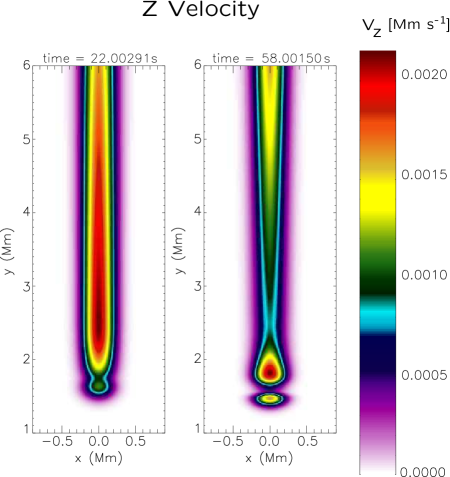
Figure 2: Transverse velocity $V_{\rm z}$ profiles at $t=22$ s and $t=58$ s for $A_{\rm v}=5$ km s^-1.

Figure 3: Results of the numerical simulation of pulse-driven linear and non-linear Alfvén waves in the coronal funnels: Time-signatures of $\rho$, $V_{\rm y}$ and $V_{\rm z}$ for $A_{\rm v}=5$ km s^-1 (left column), $A_{\rm v}=10$ km s^-1 (middle column) and $A_{\rm v}=40$ km s^-1 (right column) collected at $(x=0,y=51)$ Mm.

First, we consider the pulse amplitude $A_{\rm v}=5$ km s^-1 for the simulation of the pulse-driven linear Alfvén waves in the coronal funnel. Perturbations in $V_{\rm z}$ propagate along magnetic field lines, what is displayed on spatial profiles of $V_{\rm z}$ at $t=22$ s and $58$ s (Fig. 2). A part of the whole simulation region is illustrated in the figure. The initial pulse launched at $y_{\rm 0}=1.75$ Mm decouples into two counter-propagating waves. The amplitude of downwardly propagating waves falls off in time and these waves subside. On the other hand, upwardly propagating Alfvén waves experience an acceleration at the transition region as $c_{A}(y)$ increases up to $1$ Mm s^-1 there (Fig. 1, right) and their profile become elongated along the vertical direction. Above the transition region, Alfvén waves propagate with a constant amplitude and velocity. A part of the wave signal reflected at the transition region is well seen at $y\sim 2$ Mm at $t=58$ s (Fig. 2, right panel).

Panels in the left column of Fig. 3 illustrate typical features of the linear Alfvén wave. Here, the profiles of the mass density and $y$-component of velocity exhibit only small variations in time. The growth of $V_{\rm y}$ is by two orders of magnitude smaller than transverse velocity and it is directly associated with the Alfvén waves, which reach the detection point $(x=0\,{\rm Mm},y=51\,{\rm Mm})$ at $t\sim 55$ s. The mass density profiles exhibit a negligible decline during Alfvén wave passing. It is significant that the Alfvén waves while pass through the solar atmosphere experience a compact shape (Fig. 3, bottom panels).

The time-signature of $V_{\rm z}(x=0\,{\rm Mm},y=51\,{\rm Mm})$ for $A_{\rm v}=5$ km s^-1, illustrated in Fig. 3 (bottom-left panel), found to be similar to that obtained by Murawski & Musielak [29] [cf, their Fig. 6].

In the middle column of Fig. 3, the time-signatures of Alfvén waves, which are launched by the initial pulse with $A_{\rm v}$ = 10 km s^-1 are presented. Note that the time-signature of Alfvén waves for $A_{\rm v}=10$ km s^-1 has a similar form as in the linear case. However, the wave intensifies and enhances the plasma flows also along $y$-direction (Fig. 3, middle-center panel) two times in comparison to pulse with $A_{\rm v}=5$ km s^-1.

We also simulate the Alfvén wave using the large transversal pulse $A_{\rm v}=40$ km s^-1 that generates the large-amplitude, non-linear Alfvén waves [22] to make comparison with Alfvén waves driven by two other pulses. The time-signatures of V_z for $A_{\rm v}$ = 40 km s^-1 collected at ($x$ = 0, $y$ = 51) Mm are shown in the right column of Fig. 3. This wave experiences non-linear effects, as a result of which the vertical flows (Fig. 3, middle-right panel) are driven by a ponderomotive force.

The time-signature of $V_{\rm z}$ exhibits a double peak shape. This deformation arises as a result of partial reflection of the Alfvén waves from the transition region. The reflected signal reaches a dense photospheric plasma and reflects back towards the solar corona. For a larger initial pulse amplitude this effect is more important. Note, that even for Alfvén waves triggered by the pulse amplitude $A_{\rm v}$ = 10 km s^-1 the Gaussian shape of the wave signal is deformed on its right side (Fig. 3, bottom-middle panel).

In general, time-signatures of large-amplitude Alfvén waves exhibit similar behaviour as of the linear Alfvén wave with $A_{\rm v}=5$ km s^-1. We observe effects of the non-linear Alfvén wave decoupling from magnetoacoustic waves in $V_{\rm y}$ which magnitude grows with $A_{\rm v}$. The spatial profile of $V_{\rm y}$ for $A_{\rm v}=40$ km s^-1 (Fig. 3, middle-right panel) is like for $A_{\rm v}=5$ km s^-1 or $A_{\rm v}=10$ km s^-1, although in the case (c) it is forty times bigger than in the linear case, (a) and suffer deformation coming from a partial reflection of the Alfvén wave at the transition region.

Note that the mass density variations for Alfvén waves triggered by the initial pulses with $A_{\rm v}=5$ km s^-1, $A_{\rm v}=10$ km s^-1 and $A_{\rm v}=40$ km s^-1 (cf. Fig. 3, top panels) are insignificantly small, in particular for case (a) and (b), which are two times smaller in comparison to the case (c).

4 Discussion and Conclusions

In our pulse driven Alfvén wave model, the pulse of a small and large amplitudes are launched above the solar photosphere in the weakly expanding coronal funnels. The pulse splits into the upward and backward propagating wavetrains in the overlying solar atmosphere. The upward moving pulse train results in the instantaneous displacement of the field lines in perpendicular plane away and towards the line-of-sight. This effect generates the transverse velocity. The pulse driven linear ($A_{\rm v}=5$ km s^-1) and non-linear ($A_{\rm v}=10$ km s^-1 and $A_{\rm v}=40$ km s^-1 ) Alfvén waves exhibit different contributions in the transverse velocity V_z component at a particular height, and therefore they can play different roles in the local energy budget of the solar atmosphere. A typical granular motions can freely trigger the linear Alfvén wave with pulse amplitude $A_{\rm v}=5$ km s^-1. Whereas a generation of non-linear Alfvén wave is possible in processes of microscopic magnetic reconnection like micro- or nano-flares, where released kinetic energy disturb plasma in velocity generating MHD waves [38].

In theory, the maximum energy flux density carried out by such Alfvén waves under Wentzel-Kramers-Brillouin (WKB) approximation is [39]

$$F\approx\rho\times V_{z}^{2}\times C_{A}\,,$$ (16)

where $\rho$ is the density at the particular height, while the C_A is the local phase speed of the Alfvén waves. It should be noted that we do not calculate the energy flux distribution per degree of freedom, as we generalize the magnetic field configuration where such modes are excited. For the linear Alfvén waves ($A_{\rm v}=5$ km s^-1) in the coronal funnel, and by considering $\rho_{e}$=0.323$\times$10^-15 g cm^-3, V_z=10 km s^-1 (cf., Fig. 3, left column) as well as C_A=10³ km s^-1 at $y$=51 Mm (1.07 Ro) in the inner part of the coronal funnel, we can estimate the maximum energy flux carried out by such waves as F_max$\approx$3.0$\times$10⁴ ergs cm^-2 s^-1.

If the coronal funnel of the similar physical and magnetic field configuration exists in the polar coronal holes, then the energy carried out by such impulsively excited Alfvén waves will almost be sufficient to fulfill the energy requirement of the inner corona [39]. If the coronal funnel will be existing in the quiet-Sun or in form of active region loop arches, then such waves may only partially fulfill the energy requirements. For the non-linear Alfvén waves ($A_{\rm v}=10$ km s^-1) in the coronal funnels, and by considering $\rho_{e}$= 0.321$\times$10^-15 g cm^-3, V_z=20 km s^-1 (cf., the middle column in Fig. 3) as well as C_A=10³ km s^-1 at $y$=51 Mm (1.07 Ro) in its inner part, we can estimate the maximum energy flux carried out by such waves as F_max$\approx$1.3$\times$10⁵ ergs cm^-2 s^-1. This wave energy flux will be sufficient to fulfill the energy requirement of the inner corona [40]. However, for the coronal funnel that exists in form of active region loop arches, the computed wave energy flux only partially fulfills the required energy budget of the corona.

Now, for the non-linear Alfvén waves ($A_{\rm v}=40$ km s^-1) in the coronal funnels, and by considering $\rho_{e}$= 0.325$\times$10^-15 g cm^-3, V_z=60 km s^-1 (cf., Fig. 3, right column) as well as C_A=10³ km s^-1 at a height of 51 Mm (1.07 Ro) in its inner part, we can estimate the maximum energy flux carried out by such waves as F_max$\approx$1.2$\times$10⁶ ergs cm^-2 s^-1, which can again be sufficient to fulfill the energy requirement of the inner corona [40]. Chmielewski et al. [22] studied in details the role of such non-linear Alfvén waves in the polar coronal holes and their role in the observed spectral line broadening.

It should be noted that our calculation of the WKB part of the energy are performed only to make comparison with the wave energy computed for the linear waves. However, applications of the WKB method are limited because of abrupt variations of the plasma parameters in the stratified solar atmosphere whose spatial scales can be at a comparable magnitude to a typical wavelength. Nevertheless, we apply the WKB method in the linear regime, i.e. we ignore the higher order terms, which are related to higher-order mass density variations. As a result, we even underestimate the energy flux evaluations and the non-linear high-amplitude Alfvén waves are sufficient to fulfill the localized coronal energy losses.

In conclusion, we showed that the linear pulse-driven Alfvén waves can sufficiently power the inner corona above the polar coronal holes (for $A_{\rm v}=5$ km s^-1), while the non-linear waves (for $A_{\rm v}=10$ km s^-1 carry enough energy to fulfill the energy requirement in solar coronal holes as well as quiet-Sun energy losses. Our results clearly demonstrated that non-linear Alfvén waves ($A_{\rm v}=40$ km s^-1) can power the inner corona in the expanding coronal funnels existing anywhere, in the coronal holes, quiet-Sun, as well as in form of active region fan-like loop arches. In general Alfvén wave dissipation occurs either in the distant part of the corona [41], or by some unique processes (e.g., phase-mixing, resonant absorption) in the solar atmosphere [42,43]. Therefore, the lower part of the solar atmosphere above the polar corona may be the ideal place for the undamped growth of linear and non-linear Alfvén waves, and sufficiently large amplitude Alfvén waves may supply (and damp) their energy in the outer part of the corona and can heat the solar wind ions [44].

In the corona, the linear (e.g., $A_{\rm v}=5$ km s^-1) and non-linear Alfvén waves (e.g., $A_{\rm v}=40$ km s^-1) can carry sufficient amount of energy, and provide momentum to accelerate the solar wind plasma along the expanding magnetic field lines of the coronal funnels (e.g., coronal hole, and quiet-sun flux-tubes, respectively) [13]. Despite of polar coronal holes and quiet-Sun open magnetic field structures, the solar wind outflows and large-scale flows are also observed in the open magnetic arches near the boundary of the active regions [45]. Therefore, the large-amplitude, non-linear, pulse-driven Alfvén waves can provide sufficient energy to such kind of flows above the active regions in the expanding coronal funnels.

Acknowledgments This work has been supported by NSF under the grant AGS 1246074 (K.M. & Z.E.M.) and by the Alexander von Humboldt Foundation (Z.E.M.). The software used in this work was in part developed by the DOE-supported ASCI/Alliance Center for Astrophysical Thermonuclear Flashes at the University of Chicago. A.K.S. thanks Shobhna Srivastava for patient encouragement. AKS acknowledges the financial support from DST-RFBR-P117 project.

References

- [1] B.N. Dwivedi, A.K. Srivastava, Curr. Sci. 98, 295 (2010).
- [Alfvén(1942)] H. Alfvén, Nature 405, 150 (1942).
- [Okamoto et al.(2007)] T.J. Okamoto, S. Tsuneta, T.E. Berger, K. Ichimoto, Y. Katsukawa, B.W. Lites, S. Nagata, K. Shibata, T. Shimizu, R.A. Shine, Y. Suematsu, T.D. Tarbell, A.M. Title, Science 318, 1577 (2007).
- [De Pontieu et al.(2007)] B. De Pontieu, S.W. McIntosh, M. Carlsson, V.H. Hansteen, T.D. Tarbell, C. Schrijver, A.M. Title, R.A. Shine, S. Tsuneta, Y. Katsukawa, K. Ichimoto, Y. Suematsu, T. Shimizu, S. Nagata, Sience 318, 1574 (2007).
- [Cirtain et al.(2007)] J.W. Cirtain, L. Golub, L. Lundquist, A. van Ballegooijen, A. Savcheva, M. Shimojo, E. DeLuca, S. Tsuneta, T. Sakao, K. Reeves, M. Weber, R. Kano, N. Narukage, K. Shibasaki, Science 318, 1580 (2007).
- [Erdélyi & Fedun(2007)] R. Erdélyi, V. Fedun, Science 318, 1572 (2007).
- [Van Doorsselaere et al.(2008)] T. Van Doorsselaere, V.N. Nakariakov, E. Verwichte, Astrophys. J. Lett. 676, L73 (2008).
- [Goossens et al.(2009)] M. Goossens, J. Terradas, J. Andries, I. Arregui, J.L. Ballester, Astron. Astrophys. 503, 213 (2009).
- [Goossens et al.(2012)] M. Goossens, J. Andries, R. Soler, T. Van Doorsselaere, I. Arregui, J. Terradas, Astrophys. J. 753, 111 (2012).
- [Tian et al.(2012)] H. Tian, S.W. McIntosh, T. Wang, L. Ofman, B. De Pontieu, D.E. Innes, P. Hardi Astrophys. J. 759, 144 (2012).
- [Jess et al.(2009)] D.B. Jess, M. Mathioudakis, R. Erdélyi, P.J. Crockett, F.P Keenan, D.J. Christian, Science 323, 1582 (2009).
- [Tomczyk et al.(2007)] S. Tomczyk, S.W. McIntosh, S.L. Keil, P.G. Judge, T. Schad, D.H. Seeley, J. Edmondson, Science 317, 1192 (2007).
- [Tu et al.(2005)] C.-Y. Tu, C. Zhou, E. Marsch, L.-D. Xia, L. Zhao, J.-X. Wang, K. Wilhelm, Science 308, 519 (2005).
- [Dwivedi & Srivastava(2006)] B.N. Dwivedi, A.K. Srivastava, Sol. Phys. 237, 143 (2006).
- [Srivastava & Dwivedi(2007)] A.K. Srivastava, B.N. Dwivedi, J. of Astrophys. Astron. 28, 1 (2007).
- [Hassler et al.(1990)] D.M. Hassler, G.J. Rottman, E.C. Shoub, T.E. Holzer, T.E. Astrophys. J. Lett. 348, L77 (1990).
- [Banerjee et al.(1998)] D. Banerjee, L. Teriaca, J.G. Doyle, K. Wilhelm, Astron. Astrophys. 339, 208 (1998).
- [Moran(2003)] T.G. Moran, Astrophys. J. 598, 657 (2003).
- [O’Shea et al.(2005)] E. O’Shea, D. Banerjee, J.G. Doyle, Astron. Astrophys. 436, L43 (2005).
- [Dolla & Solomon(2008)] L. Dolla, J. Solomon, Astron. Astrophys. 483, 271 (2008).
- [Bemporad & Abbo(2012)] A. Bemporad, L. Abbo, Astrophys. J. 110, 751 (2012).
- [Chmielewski et al.(2012)] P. Chmielewski, A. K. Srivastava, K. Murawski, Z. E. Musielak, Monthly Notices of the Royal Astronomical Society 428, 40 (2013).
- [Zaqarashvili et al.(2006)] T.V. Zaqarashvili, R. Oliver, J.L. Ballester, Astron. Astrophys. 456, L13 (2006).
- [Srivastava & Dwivedi(2010)] A.K. Srivastava, B.N. Dwivedi, Monthly Notices of the Royal Astronomical Society 405, 2317 (2010).
- [McAteer et al.(2003)] R.T.J. McAteer, P.T. Gallagher, D.R. Williams, M. Mathioudakis, D.S. Bloomfield, K.J.H. Phillips, F.P. Keenan, Astrophys. J. 587, 806 (2003).
- [Musielak & Moore(1995)] Z.E. Musielak, R.L. Moore, Astrophy. J. 452, 434 (1995).
- [Roberts(2004)] B. Roberts, SOHO 13 Waves, Oscillations and Small-Scale Transients Events in the Solar Atmosphere: Joint View from SOHO and TRACE 547, 1 (2004).
- [Antolin et al.(2009)] P. Antolin, K. Shibata, T. Kudoh, D. Shiota, D. Brooks, The Second Hinode Science Meeting: Beyond Discovery-Toward Understanding 415, 247 (2009).
- [Murawski & Musielak(2010)] K. Murawski, Z.E. Musielak, Astron. Astrophys. 518, A37 (2010).
- [Verdini & Velli(2007)] A. Verdini, M. Velli, Astrophys. J. 662, 669 (2007).
- [Verdini et al.(2009)] A. Verdini, M. Velli, E. Buchlin, Astrophys. J. Lett. 700, L39 (2009).
- [Matsumoto & Shibata(2010)] T. Matsumoto, K. Shibata, Astrophys. J. 710, 1857 (2010).
- [Vernazza et al.(1981)] J.E. Vernazza, E.H. Avrett, R. Loeser, Astrophys. J.l Suppl. Series 45, 635 (1981).
- [Banaszkiewicz et al.(1998)] M. Banaszkiewicz, W.I. Axford, J.F. McKenzie, Astron. Astrophys. 337, 940 (1998).
- [Hackenberg et al.(2000)] P. Hackenberg, E. Marsch, G. Mann, Astron. Astrophys. 360, 1139 (2000).
- [Fryxell et al.(2000)] B. Fryxell, K. Olson, P. Ricker, F.X. Timmes, M. Zingale, D.Q. Lamb, P. MacNeice, R. Rosner, J.W. Truran, H Tufo, Astrophys. J. Suppl. Series 131, 273 (2000).
- [Toro(2006)] E.F. Toro, International Journal for Numerical Methods in Fluids 52, 433 (2006).
- [Hudson(1991)] H.S. Hudson, Sol. Phys. 133, 357 (1991).
- [Kudoh & Shibata(1999)] T. Kudoh, K. Shibata, Astrophys. J. 514, 493 (1999).
- [Withbroe & Noyes(1977)] G.L. Withbroe, R.W. Noyes, Ann. Rev. Astron. Astrophys. 15, 363 (1977).
- [Parker(1991)] E.N. Parker, Astrophys. J. 372, 719 (1991).
- [Heyvaerts & Priest(1983)] J. Heyvaerts, E.R. Priest, Astron. Astrophys. 117, 220 (1983).
- [Erdelyi & Goossens(1995)] R. Erdelyi, M. Goossens, Astron. Astrophys. 294, 575 (1995).
- [Ofman & Davila(2001)] L. Ofman, J.M. Davila, Astrophys. J. 553, 935 (2001).
- [Harra et al.(2008)] L.K. Harra, T. Sakao, C.H. Mandrini, H. Hara, S. Imada, P.R. Young, L. van Driel-Gesztelyi, D. Baker, Astrophys. J. 676, L147 (2008).