An empirical Bayes testing procedure for detecting variants in analysis of next generation sequencing data

Abstract

Because of the decreasing cost and high digital resolution, next-generation sequencing (NGS) is expected to replace the traditional hybridization-based microarray technology. For genetics study, the first-step analysis of NGS data is often to identify genomic variants among sequenced samples. Several statistical models and tests have been developed for variant calling in NGS study. The existing approaches, however, are based on either conventional Bayesian or frequentist methods, which are unable to address the multiplicity and testing efficiency issues simultaneously. In this paper, we derive an optimal empirical Bayes testing procedure to detect variants for NGS study. We utilize the empirical Bayes technique to exploit the across-site information among many testing sites in NGS data. We prove that our testing procedure is valid and optimal in the sense of rejecting the maximum number of nonnulls while the Bayesian false discovery rate is controlled at a given nominal level. We show by both simulation studies and real data analysis that our testing efficiency can be greatly enhanced over the existing frequentist approaches that fail to pool and utilize information across the multiple testing sites.

, and T2Supported in part by the National Science Foundation through major research instrumentation Grant number CNS-09-58854. t3Supported by the NSF Grant DMS-12-08735.

1 Introduction

The per-base cost of DNA sequencing has plummeted by 100,000-fold over the past decade because of the dramatic development in sequencing technology in the past few years [Lander (2011)]. As a result, this new or “next generation” sequencing (NGS) technology becomes much more affordable today. With high digital resolution, NGS is expected to replace the traditional hybridization-based microarray technology [Mardis (2011)]. For genetics studies, NGS holds the promise to revolutionize genome-wide association studies (GWAS). In the microarray era, GWAS mainly addresses common Single Nucleotide Polymorphisms (SNPs) with minor allele frequency $>$5%, based upon the common disease/common variant (CD/CV) hypothesis [Manolio et al. (2009)]. However, the identified common variants explain only a small proportion of heritability [Hindorff et al. (2009)]. Rare variants therefore have been hypothesized to account for the missing heritability [Bodmer and Bonilla (2008), Frazer et al. (2009)]. To identify rare variants, a direct and more powerful approach is to sequence a large number of individuals [Li and Leal (2009)]. This line of thought also implicitly motivates the recent 1000 Genomes Project, which will sequence the genomes of 1200 individuals of various ethnicities by NGS [Hayden (2008)]. It is expected to extend the catalogue of known human variants down to a frequency near 1%. Besides human genetics, NGS is also revolutionizing genetics in other species. For example, NGS has been used for genotyping in maize, barley [Elshire et al. (2011)] and rice [Huang et al. (2009)], accessing allele frequencies genome-wide in Drosophila [Turner et al. (2011), Zhu et al. (2012)], and quantifying strain abundance in yeast [Smith et al. (2010)]. Because of the small sizes of their genomes, whole-genome sequencing data for tens or hundreds of samples can be feasibly generated by one single sequencing run [Smith et al. (2010), Zhu et al. (2012)]. Finally, in cancer genomics, it is interesting to study the subclonal architecture of tumors. Within a single tumor, that is, just one individual, there often exists subclones of various sizes that have distinct somatic mutations. In the case of smaller subclones, their distinct variants can be present at low frequency when one sequences the tumor as a whole. To resolve these subclones, one must be able to accurately identify such low frequency variants and use them to make inferences about cellular frequency and, thus, subclonal composition. For such applications, even if one tumor (one sample) is sequenced as a whole, it actually consists of a pool of heterogeneous cells from which rare variants are sought.

Thousands of samples need to be sequenced for securing the chance of finding most rare variants with a frequency $<$1% [Li and Leal (2009)]. A cost-effective strategy is needed in order to afford very large sample sizes for finding rare variants. Similar issues of cost and labor were confronted in the early expensive stage of GWAS and were circumvented by focusing on small candidate regions and the use of genomic DNA pooling [Sham et al. (2002), Norton et al. (2004)]. Borrowing the same idea, many targeted resequencing applications utilizing pooling have been seen in the past few years [Nejentsev et al. (2009), Out et al. (2009), Calvo et al. (2010), Momozawa et al. (2011)].

Current NGS can generate up to several hundred million reads per run, which may lead to oversampling with little gain in data quality when analyzing one sample with a small genome or small targeted genomic regions. To fully exploit the high-throughput of NGS, nucleotide-based barcodes have been used to multiplex individual samples [Craig et al. (2008)]. Different from the aforementioned pooling strategy, this methodology allows to sequence multiple samples in a single flow cell while keeping sample identities. However, it should be noted that, despite the more efficient use of sequencing throughput, multiplexing techniques still require a large number of individual DNA extractions, manipulations of reagents, barcoding oligos, PCR reactions and sequencing library constructions [Zhu et al. (2012)]. For example, in one of our ongoing projects targeted resequencing 6 Mb genomic regions of 960 human samples, the cost for the library preparation kit (TruSeq Library Prep${}+{}$NimbleGen Custom EZ Seq Cap Panel) is $405 per sample (labor cost not included). We might multiplex 96 samples on one Illumina HiSeq 2000 lane and get enough sequencing depth per sample ($>$40X/sample). Although the cost for the sequencing step is then restrained to $2200 (one lane), the library preparation would cost dominantly as much as $96*405=\$38\mbox{,}880$, which is not reduced by multiplexing/barcoding. The library preparation step is cheaper for whole genome sequencing, as there is no need for capturing targeted regions. However, the total library preparation cost for multiplexing tens or more of samples on one lane is still much higher than that for the sequencing step. In contrast, pooling individuals prior to DNA extraction and sequencing the pooled DNA without barcodes are very cost-effective by reducing library preparation cost. As a result, for population studies where identifying variants and frequencies is the primary interest rather than knowing which sample the variant came from, nonindexed multi-sample pools are being widely used to discover rare variants and/or assess allele frequencies at population level in Drosophila [Kolaczkowski et al. (2011), Turner et al. (2011), Zhu et al. (2012)], Anopheles gambiae [Cheng et al. (2012)], Arabidopsis [Turner et al. (2010)], pig [Amaral et al. (2011)] and human [Margraf et al. (2011)], among others.

A schematic example of pooled NGS data is illustrated in Figure 1 assuming there are $M$ pools with $N$ samples in each pool. For most species, the genetic material DNA is identical at most bases in a population apart from variations at a small proportion of loci. Single Nucleotide Variants (SNVs) are the most common DNA sequence variations occurring when a single nucleotide (A, T, C or G) in the genome differs between members of a biological species or paired chromosomes in an individual. SNVs generally exhibit two alleles in a population. In this particular example, the two alleles, reference (major) allele and alternative (minor) allele, are A and G, respectively. Each nucleotide site in each individual chromosome is sequenced a random number of times. When pooling $N>1$ individuals, the information of which individual chromosome is represented in a particular read is lost. In addition, sequencing errors may flip the original allele into different ones that are observed. It is noted that when there is only $N=1$ individual in a “pool”, it represents so-called (individually sequenced) multiple-sample variant call. Finally, in the aforementioned cancer genomics studies, because of the heterogeneity of tumor cell population, the effective $N$ for one individual tumor sample is believed to be larger than 1.

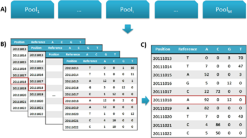
Figure 1: Schematic illustration of pooled next generation sequencing data. (A) Suppose M pools are designed for sequencing and each pool contains N samples. There are two scenarios for pooled data. When $M>1$, multiple pool sequencing data are generated. It is possible that $M>1$ and $N=1$, representing so-called (individually sequenced) multiple-sample variant call. If $M=1$, it becomes single pool data. It noted that for “one” heterogenous cancer sample, the effective $N$ is larger than 1. (B) For the $i$th pool of $N$ samples, each nucleotide site is sequenced a random number of times, which yields different counts of four nucleic acid bases (A, C, G, T) that make up DNA. (C) An example of pooling $N$ samples at a particular site. There are two types of alleles: the reference (major) allele A and the alternative (minor) allele G. The information is combined from the entire pool of n individuals.

Identification of genomic variants has become routine after NGS DNA data are generated. Quite a few tools have been implemented to identify SNVs. Formally, for a genomic locus, if its minor allele frequency (MAF) in a population is larger than 0, then we call it a SNV. SNV detection is a relatively straightforward problem in analysis of individual data, because the frequency of a candidate allele can be only 0 (nonvariant), 0.5 (heterozygous) or 1 (alternate homozygous) for a diploid genome. Several similar conventional Bayesian models have been used in existing popular tools [Li, Ruan and Durbin (2008), Li et al. (2009a, 2009b), McKenna et al. (2010)]. The multiplicity issue has been largely ignored in these conventional Bayesian approaches. Identifying variants from pooled NGS data is more challenging in that pooled DNA are sampled from a number of individuals, which consequently will give rise to variant allele frequencies other than simply 0, 0.5 or 1. Driven by the need for analysis of increasing amount of pooled NGS data, quite a few statistical models for the detection of variants from pooled sequencing data have been developed [Druley et al. (2009), Bansal (2010), Vallania et al. (2010), Altmann et al. (2011), Wei et al. (2011)]. Most existing methods, however, are based on statistical tests from a frequentist point of view. For example, Wei and colleagues propose a binomial–binomial model for testing the existence of variants from a single-pool data [Wei et al. (2011)]. Their binomial–binomial model provides a unified likelihood function for both pooled and individual data and has addressed the multiplicity issue. When there is more than one pool, they employ the partial conjunction test [Benjamini and Heller (2008)] that at least $u=1$ out of the $M$ hypotheses is false for testing whether a locus is a variant site. Alternatively, one can also combine individual pool $p$-values by conducting meta analysis. These frequentist approaches, despite making few assumptions, fail to pool and utilize information across the multiple sites that are being tested. Although these approaches are valid in terms of controlling the FDR at the nominal level, they are not optimal and powerful in detecting variants of interest. We call an FDR procedure valid, if it controls the FDR at the nominal level and optimal, if it has the smallest false negative rate [FNR, Genovese and Wasserman (2002)] among all valid FDR procedures [Wei et al. (2009)]. The optimality issue in multiple testing has received more and more attention in the past few years [Sun and Cai (2007, 2009), Wei et al. (2009), Wang, Wei and Sun (2010), He, Sarkar and Zhao (2012), Sun and Wei (2011), Xie et al. (2011)].

Hundreds of thousands or more sites are tested in typical NGS data. Such high dimensionality imposes great challenges, but can also be a blessing for inference if handled properly. Empirical Bayesian approaches, a hybrid of frequentist and Bayesian methods, become increasingly popular in modern high-dimensional data inference [Efron (2005)]. It enables the frequentists to achieve the Bayesian efficiency in solving high-dimensional problems [Efron (2010)]. Assume that the high-dimensional parameters follow some distribution governed by, for instance, a few hyperparameters. These hyperparameters can be estimated reliably via a classical frequentist way. In addition, empirical Bayesian approaches eliminate the subjective selection of priors and are generally more robust.

In this article we propose a parametric empirical Bayes testing procedure for detecting variants in the analysis of high-dimensional NGS data. When deriving our empirical Bayes procedure, we start from assuming the hyperparameters are known. Given the known hyperparameters, we derive a Bayesian decision rule which is optimal in the sense of detecting the maximum number of variants while the Bayesian false discovery rate [Sarkar, Zhou and Ghosh (2008)] is controlled at a given nominal level. To avoid a subjective choice of the hyperparameters, we estimate the hyperparameters consistently by using the method of moments, followed by an empirical Bayes procedure. Asymptotically, it is guaranteed that the empirical Bayes procedure mimics the oracle procedure uniformly for all the hyperparameters.

In this article we introduce our empirical Bayes testing procedure in Section 2. We present results from simulation studies in Section 3 to demonstrate the superiority of the proposed procedures in comparison with existing methods. In Section 4, for a case study, we apply the data-driven procedure to analyze a recent real NGS data set. We present a brief discussion in Section 5. The proof of the theorems are provided in the supplemental article [Zhao, Wang and Wei (2013)].

The methods developed in this paper have been implemented using Java in a computationally efficient and user-friendly software package, EBVariant, as well as an R package, available from http://ebvariant.sourceforge.net/.

2 Statistical models and methods

To discover (rare) variants in a cost-effective way, we consider a sequencing procedure by pooling a normalized amount of DNA from multiple samples. Because of a capacity issue, samples may be distributed and sequenced independently in more than one pools. Without loss of generality, we assume that there are $M$ pools, each pool with $N$ individuals (haploids). It is noted that the following proposed model assumes a general framework and does not require $N>1$. As a result, when $N=1$ ($N=2$ for a diploid genome), implying each pool has only one sample, the proposed model is still applicable and will make an individually sequenced multiple-sample variant call. Suppose that sequencing covers $p$ sites that are to be tested for variant candidates. We expect $p$ to be tens or hundreds of thousands for targeted resequencing, millions for whole-exome sequencing, and billions for whole-genome sequencing (human). We assume that $K_{ij}$ short reads cover locus $i$ in pool $j$, out of which we observe $X_{ij}$ reads carry alternative alleles. If there were no sequencing and mapping errors, we might easily identify variant loci as those with $X_{ij}>0$. We assume a general sequencing/mapping error $\varepsilon$, under which the alternative allele will be flipped to one of the other three alternate alleles, and vice versa. Our goal is to identify single nucleotide variants (SNVs) that have nonzero minor allele frequencies in the population.

2.1 Oracle testing procedure for multiple pools

We assume that $\theta_{ij}$ is the minor (alternative) allele frequency (MAF) at the $i$th site in the $j$th pool. Let $\mu_{i}\in\{0,1\}$ be the hidden state of whether the $i$th locus is a SNV. Given $\mu_{i}=0$, then $\theta_{ij}=0,\forall j=1,2,\ldots,M$. If $\mu_{i}=1$, then $\theta_{ij}$’s are nonzero but may vary across different pools. Following a binomial–binomial model proposed by Wei et al. (2011), we assume that the unknown MAF $\theta_{ij}$ governs $n_{ij}$, the number of haploids in a pool carrying the alternative alleles, by a binomial model; and that the unobserved $n_{ij}$ governs its proxy $X_{ij}$ by another binomial model. Unlike the frequentist approach in Wei et al. (2011), we put a prior for $\theta_{ij}$ as $\psi(\theta_{ij})$ when it is nonzero. We therefore have a hierarchical model as follows:

$$\cases{\displaystyle X_{ij}|n_{ij}\sim b\biggl{(}K_{ij},\frac{n_{ij}}{N}(1-\varepsilon)+\biggl{(}\frac{N-n_{ij}}{N}\frac{\varepsilon}{3}\biggr{)}\biggr{)},\vspace*{2pt}\cr n_{ij}|\theta_{ij}\sim b(N,\theta_{ij}),\vspace*{2pt}\cr\theta_{ij}|\mu_{i}\sim(1-\mu_{i})\delta_{0}+\mu_{i}\psi(\theta_{ij}),\vspace*{2pt}\cr\mu_{i}\sim\operatorname{Bernoulli}(\pi_{0}).}$$ (1)

When there are millions of parameters to be inferred, a common strategy is to assume that these parameters are drawn from a certain distribution. We take the parametric approach and assume that $\theta_{ij}$ follows a uniform distribution $U(0,a)$ with $0<a<1$ when $\mu_{i}=1$. The corresponding likelihood function of $X_{ij}$ ($i=1,2,\ldots,p,j=1,2,\ldots,M$) is

$$f(X_{ij}|\theta_{ij},\mu_{i}=1) = \sum_{n_{ij}=0}^{N}\pmatrix{K_{ij}\cr X_{ij}}\biggl{(}\frac{n_{ij}}{N}(1-\varepsilon)+\frac{N-n_{ij}}{N}\frac{\varepsilon}{3}\biggr{)}^{X_{ij}}$$

$$\hskip 22.0pt{}\times\biggl{(}1-\biggl{(}\frac{n_{ij}}{N}(1-\varepsilon)+\frac{N-n_{ij}}{N}\frac{\varepsilon}{3}\biggr{)}\biggr{)}^{K_{ij}-X_{ij}}$$

$$\hskip 22.0pt{}\times\pmatrix{N\cr{n_{ij}}}\theta_{ij}^{n_{ij}}(1-\theta_{ij})^{N-n_{ij}}.$$

When $\mu_{i}=0$, the likelihood function becomes

$$f(X_{ij}|\mu_{i}=0)=\pmatrix{K_{ij}\cr{X_{ij}}}\biggl{(}\frac{\varepsilon}{3}\biggr{)}^{X_{ij}}\biggl{(}1-\frac{\varepsilon}{3}\biggr{)}^{K_{ij}-X_{ij}}.$$ (3)

To identify the variants, we test the hypothesis $H_{i}\dvtx\mu_{i}=0,i=1,2,\ldots,p$. In this multiple-pool scenario, a question remains on how to combine the data from multiple pools together. Wei and colleagues test each single pool separately and combine the single-pool $p$-values using the Simes’ method for testing a partial conjunction hypothesis [Wei et al. (2011)]. Alternatively, one can conduct the meta-analysis using, for instance, Fisher’s combined probability test [Fisher (1925)]. However, none of these methods is optimal. We will show in Section 3 that these two approaches are conservative in detecting the variants. The goal of this paper is to construct an optimal multiple testing procedure by using the Bayesian decision theory [He, Sarkar and Zhao (2012), Sun and Cai (2007)].

Let $\delta_{i}$ be the 0–1 decision rule corresponding to the $i$th hypotheses, that is, we reject the hypothesis $H_{i}$ if $\delta_{i}=1$. We consider the loss function

$$L(\bolds{\delta},\bolds{\mu})=\sum_{i}\lambda(1-\mu_{i})\delta_{i}+\mu_{i}(1-\delta_{i}),$$ (4)

where the tuning parameter $\lambda$ controls the trade-off between the Type I error and the Type II error. Then to minimize the Bayes risk $EL(\bolds{\delta},\bolds{\mu})$, we have the Bayesian decision rule $\bolds{\delta}^{B}=(\delta_{1}^{B},\ldots,\delta_{p}^{B})$ with

$$\delta_{i}^{B}=I\biggl{(}P(\mu_{i}=0|\mathbf{X})<\frac{1}{\lambda+1}\biggr{)}.$$ (5)

Let $fdr_{i}(\mathbf{X})=P(\mu_{i}=0|\mathbf{X})$ be the posterior probability of $\mu_{i}$ being zero, which is the local fdr score as given in Efron et al. (2001), Efron (2008, 2010). It can be written as

$$\qquad fdr_{i}(\mathbf{X})=\frac{\pi_{0}\prod_{j=1}^{M}f(X_{ij}|\mu_{i}=0)}{\pi_{0}\prod_{j=1}^{M}f(X_{ij}|\mu_{i}=0)+\pi_{1}\prod_{j=1}^{M}\int f(X_{ij}|\theta_{ij})\psi(\theta_{ij})\,d\theta_{ij}}.$$ (6)

Unlike the two aforementioned approaches, the local fdr score combining the information across multiple pools proves optimal in the decision theoretical framework.

The Bayesian decision rule (5) depends on the tuning parameter $\lambda$ which, however, is not trivial to set. In many real applications, of interest is to control certain type I error rates. False discovery rate (FDR) [Benjamini and Hochberg (1995)] is one of the most popular ones for high-dimensional data. Its recent extensions include mFDR, which equals $\mathit{FDR}+O(1/p)$ under weak conditions [Genovese and Wasserman (2002)], and positive FDR [Storey (2003)]. Following Sarkar, Zhou and Ghosh (2008), we consider the Bayes version of FDR and FNR (false nondiscovery rate) in the Bayesian framework as follows.

Let $R=\sum_{i=1}^{p}\delta_{i}$ and $A=\sum_{i=1}^{p}(1-\delta_{i})$ be the total number of rejections and acceptances, respectively. Let $V=\sum_{i=1}^{p}\delta_{i}(1-\mu_{i})$ and $U=\sum_{i=1}^{p}\mu_{i}(1-\delta_{i})$ be the number of false rejections and false acceptances, respectively. Define BFDR and BFNR as

$$\mathit{BFDR}=E_{\mathbf{X},\bolds{\mu}}\frac{V}{R\vee 1},\qquad\mathit{BFNR}=E_{\mathbf{X},\bolds{\mu}}\frac{U}{A\vee 1}.$$

Let $t=\frac{1}{\lambda+1}$ and we rewrite the decision Bayes rule as $\bolds{\delta}^{B}(t)=(\delta_{1}^{B}(t),\ldots,\break\delta_{p}^{B}(t))$ with

$$\delta_{i}^{B}(t)=I\bigl{(}P(\mu_{i}=0|\mathbf{X})<t\bigr{)}.$$ (7)

Then

$$\mathit{BFDR}\bigl{(}\bolds{\delta}^{B}(t)\bigr{)}=E\frac{\sum_{i}I(fdr_{i}(\mathbf{X})<t)fdr_{i}(\mathbf{X})}{\sum_{i}I(fdr_{i}(\mathbf{X})<t)\vee 1},$$

which is increasing with respect to $t$. As $t\to 0$, it converges to 0. When $t\to+\infty$, then

$$\lim_{t\to+\infty}\mathit{BFDR}\bigl{(}\bolds{\delta}^{B}(t)\bigr{)}=\frac{1}{p}E_{m(\mathbf{X})}\sum_{i}fdr_{i}(\mathbf{X})=\pi_{0}.$$

Consequently, when $\pi_{0}>\alpha$, there exists a value $t(\alpha)$ such that the decision Bayes rule controls the BFDR at $\alpha$ and the BFDR is greater than $\alpha$ for any $t>t(\alpha)$. Sun and Cai (2007) and He, Sarkar and Zhao (2012) have shown that this procedure is optimal in the sense that it yields the minimal BFNR among all procedures that can control the BFDR at level $\alpha$. This optimal rule relies on the cut-off $t(\alpha)$, which depends on $\alpha$ implicitly. After deriving the empirical Bayes version of the local fdr scores in Section 2.2, we introduce a data driven procedure to choose this cutoff in Section 2.3.

2.2 Empirical Bayes estimators

The oracle testing procedure defined in Section 2.1 assumes that the hyperparameters $\pi_{0}$, $\pi_{1}$ and $a$ are known. To avoid a subjective choice of these hyperparameters, we estimate them using an empirical Bayes approach. To simplify our discussion, we first explain the estimators for the hyperparameters for single-pool data. Taking out the pool index $j$, the hierarchical model for single-pool data becomes

$$\cases{\displaystyle X_{i}|n_{i}\sim b\biggl{(}K_{i},\frac{n_{i}}{N}(1-\varepsilon)+\biggl{(}\frac{N-n_{i}}{N}\frac{\varepsilon}{3}\biggr{)}\biggr{)},\vspace*{2pt}\cr n_{i}|\theta_{i}\sim b(N,\theta_{i}),\vspace*{2pt}\cr\theta_{i}|\mu_{i}\sim(1-\mu_{i})\delta_{0}+\mu_{i}U(0,a),\vspace*{2pt}\cr\mu_{i}\sim\operatorname{Bernoulli}(\pi_{0}).}$$ (8)

Define two statistics

$$m_{1}=\frac{\sum_{i}(X_{i}/K_{i}-{\varepsilon}/{3})}{p}$$ (9)

and

$$m_{2} = \frac{1}{p}\sum_{i}\bigl{(}X_{i}^{2}-K_{i}^{2}\bigl{(}{\varepsilon^{2}}/{9}\bigr{)}-K_{i}({\varepsilon}/{3})\bigl{(}1-({\varepsilon}/{3})\bigr{)}-K_{i}\bigl{(}1-({2\varepsilon}/{3})\bigr{)}m_{1}$$

$$\hskip 224.0pt{}-K_{i}^{2}({2\varepsilon}/{3})m_{1}\bigr{)}$$

$$\hskip 26.0pt{}/{\bigl{(}\bigl{(}K_{i}^{2}-K_{i}\bigr{)}(1-{4\varepsilon}/{3})^{2}\bigr{)}}.$$

Theorem 2.1

Assume the model (8) and the definitions of $m_{1}$ and $m_{2}$ in (9) and (2.2), then

$$Em_{1}=\biggl{(}1-\frac{4\varepsilon}{3}\biggr{)}\pi_{1}\frac{a}{2}$$

and

$$Em_{2}=\frac{N-1}{N}\pi_{1}\frac{a^{2}}{3}+\frac{1}{N}\pi_{1}\frac{a}{2}.$$

By using the method of moments, we can estimate $a$, $\pi_{0}$ and $\pi_{1}$ as

$$\cases{\displaystyle\hat{a}=\frac{3(N(1-{4\varepsilon}/{3})m_{2}-m_{1})}{2m_{1}(N-1)},&\vspace*{2pt}\cr\displaystyle\hat{\pi}_{1}=\frac{2m_{1}}{(1-{4\varepsilon}/{3})\hat{a}},&\quad$\hat{\pi}_{0}=1-\hat{\pi}_{1}.$}$$ (11)

Theorem 2.2

Assume that the empirical Bayes estimators of $a$, $\pi_{0}$ and $\pi_{1}$ are given by (11), then $\hat{a}\stackrel{{\scriptstyle\mathrm{P.}}}{{\to}}a$, $\hat{\pi}_{0}\stackrel{{\scriptstyle\mathrm{P.}}}{{\to}}\pi_{0}$ and $\hat{\pi}_{1}\stackrel{{\scriptstyle\mathrm{P.}}}{{\to}}\pi_{1}$, for all $0<a<1,0<\pi_{1}<1$.

The estimation of these hyperparameters borrows information across all loci and is thus consistent when the number of loci goes to infinity. This can be viewed as the blessing of the high dimensionality. It is noted that the estimation may result in negative estimates of $a$ and $\pi_{1}$ when $p$ is finite. For NGS data analysis, people may have certain knowledge about these unknown parameters. For example, genome-wide $\pi_{1}$ is believed to be greater than 0.1%. We then can set $\hat{\pi}_{1}$ as 0.1% if it is less than 0. Similarly, we may estimate $a$ as $0.01$ if $\hat{a}<0$. Therefore, we have the truncated estimators for the hyperparameters as

$$\cases{\hat{a}^{T}=\hat{a}I(\hat{a}>0)+0.01I(\hat{a}<0),\vspace*{2pt}\cr\hat{\pi}_{1}^{T}=\hat{\pi}_{1}I(\hat{\pi}_{1}>0)+0.001I(\hat{\pi}_{1}<0),\qquad\hat{\pi}_{0}^{T}=1-\hat{\pi}_{1}^{T}.}$$ (12)

These truncated estimators are still consistent for $\pi_{0}\in(0,1)$ and $a\in(0,1)$.

For the multiple-pool scenario as described in model (1), we assume the observations $X_{ij},i=1,2,\ldots,p,j=1,2,\ldots,M$, share the same marginal distribution. Treating $\{X_{ij}\}$ and $\{K_{ij}\}$ as $p\times M$-dimensional vectors, we can estimate $\pi_{1}$ and $a$ by (12) similarly. Such estimators converge even faster because of the larger sample size.

2.3 An empirical Bayes testing procedure

Section 2.1 has developed an optimal oracle testing procedure. Section 2.2 has provided the empirical Bayes estimators for the parameters $\pi_{0}$ and $a$ in the testing procedure when they are unknown. In this section we propose an empirical Bayes testing procedure as follows.

Definition 2.1 ([An Empirical Bayes Testing Procedure (emBayes)]).

[1.]

Estimate $\pi_{0}$ and $a$ according to (12).

For the $i$th locus, calculate the local fdr $\widehat{fdr_{i}(X)}$ by plugging the $\hat{\pi}_{1}$ and $\hat{a}$ into (6).

Order $\widehat{fdr_{i}(X)}$ as $\widehat{fdr_{(1)}(X)}\leq\widehat{fdr_{(2)}(X)}\leq\cdots\leq\widehat{fdr_{(p)}(X)}$.

Find the maximum $J$ such that $\frac{1}{J}\sum_{i=1}^{J}\widehat{fdr_{(i)}(X)}\leq\alpha$.

Reject hypothesis $H_{(1)},H_{(2)},\ldots,H_{(J)}$ and accept the rest.

Theorem 2.3

Assume the model (1) and the hyperparameters are estimated as described in Section 2.2. Let $\widetilde{\mathit{BFDR}}$ and $\widetilde{\mathit{BFNR}}$ be the Bayes FDR and FNR of the empirical Bayes procedure. Then

$$\widetilde{\mathit{BFDR}}=\mathit{BFDR}_{\mathrm{OR}}+o(1),\qquad\widetilde{\mathit{BFNR}}=\mathit{BFNR}_{\mathrm{OR}}+o(1)$$

for any $\pi_{1}\in(0,1)$ and $a\in(0,1)$, where $\mathit{BFDR}_{\mathrm{OR}}$ and $\mathit{BFNR}_{\mathrm{OR}}$ are the Bayes FDR and FNR of the oracle optimal multiple testing procedure.

The empirical Bayes procedure was first introduced by Robbins (1951, 1956), and is also known as a nonparametric empirical Bayes procedure because the prior is completely unspecified. Recently, Sun and Cai (2007) and He, Sarkar and Zhao (2012) constructed optimal nonparametric empirical Bayes multiple testing procedures in the normal mean setting. In our study, the observation follows a binomial–binomial model. We put a family of priors with a few hyperparameters for governing the high-dimensional parameters. The resultant approach is a parametric empirical Bayes procedure, first proposed by Efron and Morris (1971, 1973, 1975). Asymptotically, the procedure controls the Bayes FDR uniformly for all hyperparameter settings. This control is less stringent than that in the frequentist procedure which requires that the Bayes FDR be controlled for the class of all point priors on $\theta$ [Morris (1983)]. Our empirical Bayes procedure is more robust than the conventional Bayesian approach which takes a subjective choice of the hyperparameters. For instance, when setting $\pi_{1}$ as 0.4%, the conventional Bayesian procedure may not control the BFDR if the true $\pi_{1}$ is less than 0.4%, and it may lack power if the true $\pi_{1}$ is greater than 0.4%.

3 Simulation

We first investigate the numerical performance of the proposed empirical Bayes procedure (emBayes) using simulated data. Simulation design follows Wei et al. (2011), with the settings: $M=5$ pools, $N=20$ subjects in each pool, the proportion of alternatives $\pi_{1}$ varying among 1%, 0.7%, 0.3% and 0.1%, the MAF $\psi(\theta_{ij})\sim U(0,a)$ with $a$ being 0.01, 0.02, 0.03 or 0.05, the number of loci $p=1$ million (1M) or 2 millions (2M), the sequencing error $\varepsilon=0.01$, and the sequencing coverage $K_{ij}$ following a gamma distribution with mean 30 [Prabhu and Pe’er (2009)].

We compare emBayes with its oracle version, where we use the true values of $a$ and $\pi_{0}$, and two frequentist approaches, SNVer and META. Both SNVer and META test each single pool separately using the binomial–binomial model. SNVer [Wei et al. (2011)] combines the single-pool $p$-values using the Simes’ method for testing a partial conjunction hypothesis in order to get multiple-pool $p$-values. META conducts meta-analysis and obtains multiple-pool $p$-values as

$$p^{\mathrm{Pool}}=P\Biggl{(}\chi^{2}_{2M}>-2\sum_{j=1}^{M}\ln{p_{j}}\Biggr{)},$$

where $\chi^{2}_{2M}$ is the chi-squared random variable with $2M$ degrees of freedom. Both approaches then employ the BH procedure [Benjamini and Hochberg (1995)] to control FDR.

We evaluate these methods by the number of total rejections (ER), the number of false rejections (EV) and the FDR, averaged over 100 replications, at the nominal FDR level 0.05. The results are summarized in Table 1. Compared with SNVer, META is more conservative and dominated, as indicated by its smaller FDR, fewer total rejections and fewer true rejections. The results for META are thus not included in the table.

Table 1: The power and FDR comparison of emBayes, SNVer and the oracle procedure at the nominal FDR level $5\%$. ER: the number of total rejections; EV: the number of false rejections; FDR: false discovery rate

			emBayes		Oracle		SNVer
$\bolds{\pi_{1}}$	a	p	ER/EV	FDR	ER/EV	FDR	ER/EV	FDR
$\pi_{1}=1\%$	0.01	1$M$	467/20	$0.039$	541/27	$0.05$	277/3.3	$0.012$
		2$M$	1058/52	$0.049$	1088/55	$0.05$	563/6.7	$0.012$
	0.02	1$M$	1464/73	$0.05$	1467/74	$0.05$	850/11	$0.013$
		2$M$	2931/144	$0.049$	2943/147	$0.05$	1702/22	$0.013$
$\pi_{1}=0.7\%$	0.01	1$M$	295/12	$0.038$	341/17	$0.049$	178/2.2	$0.012$
		2$M$	632/28	$0.042$	682/33	$0.049$	351/4.2	$0.012$
	0.02	1$M$	959/48	$0.05$	962/48	$0.05$	533/6.6	$0.012$
		2$M$	1917/94	$0.049$	1931/97	$0.05$	1063/13	$0.012$
$\pi_{1}=0.4\%$	0.01	1$M$	132/4.3	$0.029$	160/7.4	$0.046$	83/0.9	$0.010$
		2$M$	292/12	$0.04$	325/16	$0.049$	170/2.1	$0.012$
	0.02	1$M$	470/22	$0.047$	487/24	$0.049$	257/3.1	$0.012$
		2$M$	971/48	$0.049$	985/49	$0.05$	520/6.2	$0.012$
$\pi_{1}=0.1\%$	0.01	1$M$	22/1.1	$0.041$	26/1.4	$0.051$	13/0.14	$0.01$
		2$M$	44/1.8	$0.032$	55/2.4	$0.044$	26/0.18	$0.0068$
	0.02	1$M$	73/3	$0.036$	88/4.4	$0.05$	45/0.6	$0.013$
		2$M$	153/6	$0.035$	177/8.3	$0.047$	90/0.91	$0.0099$

From Table 1 we can see that the FDR levels of all three procedures are controlled at 0.05 asymptotically under all settings while SNVer is conservative. The power of emBayes is greatly improved over SNVer. For instance, when $p=1M$, $\pi_{1}=0.4\%$ and $a=0.02$, the numbers of correctly rejected hypotheses for these two approaches are 470 and 257, respectively. The number of true rejections is almost doubled. The emBayes has very comparable, if not the same, performance, compared with the oracle procedure. The discrepancy is more noticeable when $\pi_{1}$ and $a$ are smaller. The reason is that the empirical Bayes estimators of the hyperparameters converge slowly near the boundary of the parameter space.

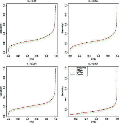
Figure 2: ROC curves to compare ranking efficiency of emBayes (red solid), SNVer (green dashed), META (blue dotted) and oracle procedure (black-dot dashed) under the setting of $p=$1$M$ and $a=0.02$ with different proportions of nonnulls.

In all these simulations, SNVer proves conservative as indicated by extremely low FDR. It is tempting to conjecture that the higher power of emBayes is gained at the price of a higher FDR level. In other words, these two methods might actually yield similar rankings of the candidate loci and would demonstrate comparable power at the same empirical FDR level. To clarify the superiority in terms of prioritizing candidate loci, we employed ROC curves to illustrate ranking efficiency. Specifically, we calculated sensitivity as the average proportions of the total number of true rejections to the total number of nonnulls over the 100 replications. We varied the significance thresholds for identifying up to 10,000 variants and calculated corresponding FDRs and sensitivities. The resultant ROC curves of sensitivity versus FDR for emBayes, SNVer, META and the oracle procedure under the setting of $p={}$1$M$ and $a=0.02$ are shown in Figure 2. It is clearly seen that emBayes dominates SNVer and META. Our proposed empirical Bayes approach can identify more true variants than the frequentist competitors at the same FDR levels. For example, when $a=0.02$, $\pi_{1}=0.1$% and the FDR level of 0.1, the numbers of true rejections for emBayes, SNVer, META and the oracle procedure are 98, 80, 81 and 98, respectively. The improvement of emBayes over SNVer is as large as $(98-80)/80=22.5$%.

In summary, our simulation studies show that not only can emBayes control FDR at nominal level, but, more importantly, it also proves optimal in terms of power and can detect more variants than its frequentist alternatives.

4 Real data analysis

We also assess the performance of our proposed approach by analyzing a real NGS data set. In a recent pooled sequencing study, Zhu and colleagues conducted whole-genome resequencing pools of nonbarcoded Drosophila melanogaster strains [Zhu et al. (2012)]. The library A (SRR353364.1) in their study was constructed from a pool of 220 flies (10 females per strain) and sequenced on a single lane of Illumina GAIIx platform with 100 bp paired-end reads, leading to an averaged sequencing depth of 10X. This library was also independently sequenced by the Drosophila Population Genomics Project (DPGP) (http://www.dpgp.org/). Following the authors, we utilized this library to evaluate variant call performance. Specifically, we extracted the genotypes of those 22 strains in the Library A from the Drosophila Genetic Reference Panel (DGRP) (http://dgrp.gnets. ncsu.edu) and used them as gold standard for estimating False Discovery Rate (FDR).

We downloaded the given bam file, based on which we then called variants using emBayes and SNVer at the nominal FDR level 0.05. Because of the large size of Drosophila genome, we analyzed the data separately for each chromosome. The variant call results are displayed in Figure 3. The emBayes called significantly more varaints than SNVer across all five chromosomes, with an average of 97,000 variants per chromosome and the improvement ranging from 13.78% (Chromosome 2L) to 17.4% (Chromosome 3R). Although, as expected, emBayes identified more variants than SNVer, it is also important to check if these two methods can control FDR at the prespecified nominal level. The majority of the called variants (89%) were found to have their genotype information available from DGRP, which were then used for estimating FDR. As we can see from Figure 3, both of the two methods controlled FDR at the nominal level, while SNVer revealed a little more conservative than emBayes. Consistent to the simulation studies, the larger numbers of variants called by emBayes therefore support its improved power over SNVer.

In summary, the real data analysis confirms that the proposed empirical Bayesian method, while addressing the multiplicity issue by controlling FDR, is a more powerful approach by utilizing the global information than the frequentist approach in detecting variants in NGS study.

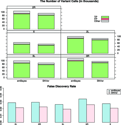
Figure 3: Variant call performance. For both methods emBayes and SNVer, we call variants at the nominal level $\alpha=0.05$. TP: True Positive; FP: False Positive. TP and FP are the variants that are called by the method and also have genotype information available from another data source (DGRP). Other: the variants called by the method but without genotype information available from DGRP. FDR: estimated false discovery rate equal to FP/(TP${}+{}$FP). emBayes calls more variants ($>$10%) than SNVer across all five chromosomes. Both methods can control FDR at the nominal level, while SNVer is more conservative than emBayes.

5 Conclusion and discussion

This paper has derived an optimal empirical Bayes testing procedure for detecting variants in analysis of the increasingly popular NGS data. We utilize the empirical Bayes technique to exploit the across-site information among the vast amount of testing sites in the NGS data. We prove that our testing procedure is valid and optimal in the sense of rejecting the maximum number of nonnulls while the marginal FDR is controlled at a given nominal level. We show by both simulation studies and real data analysis that our testing efficiency can be greatly enhanced over the existing frequentist approaches that fail to pool and utilize information across the multiple testing sites.

The existing approaches for variant call in NGS study are either conventional Bayesian models or frequentist tests. Our empirical Bayes approach can be viewed as a hybrid of the frequentist and Bayesian methods. It thus enjoys the pros of both and overcomes the cons of each. Compared to the frequentist approaches, it enjoys the Bayesian advantage of its capability of pooling information across testing sites, and therefore is more powerful. In addition, its output local fdr scores can be used as variant call quality that may be useful in downstream association analysis [Daye, Li and Wei (2012)]. Compared to the conventional Bayesian approaches, it avoids any subjective choice of prior parameters and estimates them reliably via a classical frequentist way; it gains multiplicity control by controlling the Bayes FDR at any designated level uniformly for all the hyperparameters. This is particularly desirable because tens of thousands or millions of loci are simultaneously examined in typical NGS experiments. Each user can choose the false-positive error rate threshold he or she considers appropriate, instead of just the dichotomous decisions of whether to “accept or reject the candidates” provided by most existing methods.

Our current empirical Bayes testing procedure can be extended and improved in several ways. First, sequencing/mapping error in NGS data is much more complicated. Due to the heterogeneity of DNA, such as repeats, duplication and GC content, there could be distinct error profiles for different genomic regions even if they are sequenced under the same experimental condition. Instead of assuming a global and general error rate, we may take and estimate specific and local error rates empirically from the data for further improving variant call efficiency. Second, strand bias is an issue observed in many sequencing platforms but not yet considered in our testing model. We may count and model ACGT for the forward strand and reverse strand separately, so as to detect the strand bias and/or allele imbalance issues introduced by inaccurate mapping or sequencing error. Third, besides single nucleotide variants (SNVs), there exist small insertions and deletions (indels). The prevalence and distribution of these indels are quite different from SNVs. A similar empirical Bayes model but with different priors may be developed. How to combine them for an overall multiplicity control while maintaining optimality is not clear. The recent pooled analysis idea for multiple-testing in GWAS [Wei et al. (2009)] may be borrowed and worthy of further research. We are currently working on these extensions.

References

- Altmann et al. (2011) {barticle}[pbm] \bauthor\bsnmAltmann, \bfnmAndre\binitsA., \bauthor\bsnmWeber, \bfnmPeter\binitsP., \bauthor\bsnmQuast, \bfnmCarina\binitsC., \bauthor\bsnmRex-Haffner, \bfnmMonika\binitsM., \bauthor\bsnmBinder, \bfnmElisabeth B.\binitsE. B. and \bauthor\bsnmMüller-Myhsok, \bfnmBertram\binitsB. (\byear2011). \btitlevipR: Variant identification in pooled DNA using R. \bjournalBioinformatics \bvolume27 \bpagesi77–i84. \biddoi=10.1093/bioinformatics/btr205, issn=1367-4811, pii=btr205, pmcid=3117388, pmid=21685105 \bptokimsref \endbibitem
- Amaral et al. (2011) {barticle}[pbm] \bauthor\bsnmAmaral, \bfnmAndreia J.\binitsA. J., \bauthor\bsnmFerretti, \bfnmLuca\binitsL., \bauthor\bsnmMegens, \bfnmHendrik-Jan\binitsH.-J., \bauthor\bsnmCrooijmans, \bfnmRichard P. M. A.\binitsR. P. M. A., \bauthor\bsnmNie, \bfnmHaisheng\binitsH., \bauthor\bsnmRamos-Onsins, \bfnmSebastian E.\binitsS. E., \bauthor\bsnmPerez-Enciso, \bfnmMiguel\binitsM., \bauthor\bsnmSchook, \bfnmLawrence B.\binitsL. B. and \bauthor\bsnmGroenen, \bfnmMartien A. M.\binitsM. A. M. (\byear2011). \btitleGenome-wide footprints of pig domestication and selection revealed through massive parallel sequencing of pooled DNA. \bjournalPLoS ONE \bvolume6 \bpagese14782. \biddoi=10.1371/journal.pone.0014782, issn=1932-6203, pmcid=3070695, pmid=21483733 \bptokimsref \endbibitem
- Bansal (2010) {barticle}[pbm] \bauthor\bsnmBansal, \bfnmVikas\binitsV. (\byear2010). \btitleA statistical method for the detection of variants from next-generation resequencing of DNA pools. \bjournalBioinformatics \bvolume26 \bpagesi318–i324. \biddoi=10.1093/bioinformatics/btq214, issn=1367-4811, pii=btq214, pmcid=2881398, pmid=20529923 \bptokimsref \endbibitem
- Benjamini and Heller (2008) {barticle}[mr] \bauthor\bsnmBenjamini, \bfnmYoav\binitsY. and \bauthor\bsnmHeller, \bfnmRuth\binitsR. (\byear2008). \btitleScreening for partial conjunction hypotheses. \bjournalBiometrics \bvolume64 \bpages1215–1222. \biddoi=10.1111/j.1541-0420.2007.00984.x, issn=0006-341X, mr=2522270 \bptokimsref \endbibitem
- Benjamini and Hochberg (1995) {barticle}[mr] \bauthor\bsnmBenjamini, \bfnmYoav\binitsY. and \bauthor\bsnmHochberg, \bfnmYosef\binitsY. (\byear1995). \btitleControlling the false discovery rate: A practical and powerful approach to multiple testing. \bjournalJ. R. Stat. Soc. Ser. B Stat. Methodol. \bvolume57 \bpages289–300. \bidissn=0035-9246, mr=1325392 \bptokimsref \endbibitem
- Bodmer and Bonilla (2008) {barticle}[pbm] \bauthor\bsnmBodmer, \bfnmWalter\binitsW. and \bauthor\bsnmBonilla, \bfnmCarolina\binitsC. (\byear2008). \btitleCommon and rare variants in multifactorial susceptibility to common diseases. \bjournalNat. Genet. \bvolume40 \bpages695–701. \biddoi=10.1038/ng.f.136, issn=1546-1718, mid=UKMS1904, pii=ng.f.136, pmcid=2527050, pmid=18509313 \bptokimsref \endbibitem
- Calvo et al. (2010) {barticle}[pbm] \bauthor\bsnmCalvo, \bfnmSarah E.\binitsS. E., \bauthor\bsnmTucker, \bfnmElena J.\binitsE. J., \bauthor\bsnmCompton, \bfnmAlison G.\binitsA. G., \bauthor\bsnmKirby, \bfnmDenise M.\binitsD. M., \bauthor\bsnmCrawford, \bfnmGabriel\binitsG., \bauthor\bsnmBurtt, \bfnmNoel P.\binitsN. P., \bauthor\bsnmRivas, \bfnmManuel\binitsM., \bauthor\bsnmGuiducci, \bfnmCandace\binitsC., \bauthor\bsnmBruno, \bfnmDamien L.\binitsD. L., \bauthor\bsnmGoldberger, \bfnmOlga A.\binitsO. A., \bauthor\bsnmRedman, \bfnmMichelle C.\binitsM. C., \bauthor\bsnmWiltshire, \bfnmEsko\binitsE., \bauthor\bsnmWilson, \bfnmCallum J.\binitsC. J., \bauthor\bsnmAltshuler, \bfnmDavid\binitsD., \bauthor\bsnmGabriel, \bfnmStacey B.\binitsS. B., \bauthor\bsnmDaly, \bfnmMark J.\binitsM. J., \bauthor\bsnmThorburn, \bfnmDavid R.\binitsD. R. and \bauthor\bsnmMootha, \bfnmVamsi K.\binitsV. K. (\byear2010). \btitleHigh-throughput, pooled sequencing identifies mutations in NUBPL and FOXRED1 in human complex I deficiency. \bjournalNat. Genet. \bvolume42 \bpages851–858. \biddoi=10.1038/ng.659, issn=1546-1718, mid=NIHMS228290, pii=ng.659, pmcid=2977978, pmid=20818383 \bptokimsref \endbibitem
- Cheng et al. (2012) {barticle}[pbm] \bauthor\bsnmCheng, \bfnmChangde\binitsC., \bauthor\bsnmWhite, \bfnmBradley J.\binitsB. J., \bauthor\bsnmKamdem, \bfnmColince\binitsC., \bauthor\bsnmMockaitis, \bfnmKeithanne\binitsK., \bauthor\bsnmCostantini, \bfnmCarlo\binitsC., \bauthor\bsnmHahn, \bfnmMatthew W.\binitsM. W. and \bauthor\bsnmBesansky, \bfnmNora J.\binitsN. J. (\byear2012). \btitleEcological genomics of Anopheles gambiae along a latitudinal cline: A population-resequencing approach. \bjournalGenetics \bvolume190 \bpages1417–1432. \biddoi=10.1534/genetics.111.137794, issn=1943-2631, pii=genetics.111.137794, pmcid=3316653, pmid=22209907 \bptokimsref \endbibitem
- Craig et al. (2008) {barticle}[pbm] \bauthor\bsnmCraig, \bfnmDavid W.\binitsD. W., \bauthor\bsnmPearson, \bfnmJohn V.\binitsJ. V., \bauthor\bsnmSzelinger, \bfnmSzabolcs\binitsS., \bauthor\bsnmSekar, \bfnmAswin\binitsA., \bauthor\bsnmRedman, \bfnmMargot\binitsM., \bauthor\bsnmCorneveaux, \bfnmJason J.\binitsJ. J., \bauthor\bsnmPawlowski, \bfnmTraci L.\binitsT. L., \bauthor\bsnmLaub, \bfnmTrisha\binitsT., \bauthor\bsnmNunn, \bfnmGary\binitsG., \bauthor\bsnmStephan, \bfnmDietrich A.\binitsD. A., \bauthor\bsnmHomer, \bfnmNils\binitsN. and \bauthor\bsnmHuentelman, \bfnmMatthew J.\binitsM. J. (\byear2008). \btitleIdentification of genetic variants using bar-coded multiplexed sequencing. \bjournalNat. Methods \bvolume5 \bpages887–893. \biddoi=10.1038/nmeth.1251, issn=1548-7105, mid=NIHMS67302, pii=nmeth.1251, pmcid=3171277, pmid=18794863 \bptokimsref \endbibitem
- Daye, Li and Wei (2012) {barticle}[pbm] \bauthor\bsnmDaye, \bfnmZ. John\binitsZ. J., \bauthor\bsnmLi, \bfnmHongzhe\binitsH. and \bauthor\bsnmWei, \bfnmZhi\binitsZ. (\byear2012). \btitleA powerful test for multiple rare variants association studies that incorporates sequencing qualities. \bjournalNucleic Acids Res. \bvolume40 \bpagese60. \biddoi=10.1093/nar/gks024, issn=1362-4962, pii=gks024, pmcid=3340416, pmid=22262732 \bptokimsref \endbibitem
- Druley et al. (2009) {barticle}[pbm] \bauthor\bsnmDruley, \bfnmTodd E.\binitsT. E., \bauthor\bsnmVallania, \bfnmFrancesco L. M.\binitsF. L. M., \bauthor\bsnmWegner, \bfnmDaniel J.\binitsD. J., \bauthor\bsnmVarley, \bfnmKatherine E.\binitsK. E., \bauthor\bsnmKnowles, \bfnmOlivia L.\binitsO. L., \bauthor\bsnmBonds, \bfnmJacqueline A.\binitsJ. A., \bauthor\bsnmRobison, \bfnmSarah W.\binitsS. W., \bauthor\bsnmDoniger, \bfnmScott W.\binitsS. W., \bauthor\bsnmHamvas, \bfnmAaron\binitsA., \bauthor\bsnmCole, \bfnmF. Sessions\binitsF. S., \bauthor\bsnmFay, \bfnmJustin C.\binitsJ. C. and \bauthor\bsnmMitra, \bfnmRobi D.\binitsR. D. (\byear2009). \btitleQuantification of rare allelic variants from pooled genomic DNA. \bjournalNat. Methods \bvolume6 \bpages263–265. \biddoi=10.1038/nmeth.1307, issn=1548-7105, mid=NIHMS92733, pii=nmeth.1307, pmcid=2776647, pmid=19252504 \bptokimsref \endbibitem
- Efron (2005) {barticle}[mr] \bauthor\bsnmEfron, \bfnmBradley\binitsB. (\byear2005). \btitleBayesians, frequentists, and scientists. \bjournalJ. Amer. Statist. Assoc. \bvolume100 \bpages1–5. \biddoi=10.1198/016214505000000033, issn=0162-1459, mr=2166064 \bptokimsref \endbibitem
- Efron (2008) {barticle}[mr] \bauthor\bsnmEfron, \bfnmBradley\binitsB. (\byear2008). \btitleMicroarrays, empirical Bayes and the two-groups model. \bjournalStatist. Sci. \bvolume23 \bpages1–22. \biddoi=10.1214/07-STS236, issn=0883-4237, mr=2431866 \bptokimsref \endbibitem
- Efron (2010) {bbook}[mr] \bauthor\bsnmEfron, \bfnmBradley\binitsB. (\byear2010). \btitleLarge-Scale Inference: Empirical Bayes Methods for Estimation, Testing, and Prediction. \bseriesInstitute of Mathematical Statistics (IMS) Monographs \bvolume1. \bpublisherCambridge Univ. Press, \blocationCambridge. \bidmr=2724758 \bptokimsref \endbibitem
- Efron and Morris (1971) {barticle}[mr] \bauthor\bsnmEfron, \bfnmBradley\binitsB. and \bauthor\bsnmMorris, \bfnmCarl\binitsC. (\byear1971). \btitleLimiting the risk of Bayes and empirical Bayes estimators. I. The Bayes case. \bjournalJ. Amer. Statist. Assoc. \bvolume66 \bpages807–815. \bidissn=0162-1459, mr=0323014 \bptokimsref \endbibitem
- Efron and Morris (1973) {barticle}[mr] \bauthor\bsnmEfron, \bfnmBradley\binitsB. and \bauthor\bsnmMorris, \bfnmCarl\binitsC. (\byear1973). \btitleStein’s estimation rule and its competitors—An empirical Bayes approach. \bjournalJ. Amer. Statist. Assoc. \bvolume68 \bpages117–130. \bidissn=0162-1459, mr=0388597 \bptokimsref \endbibitem
- Efron and Morris (1975) {barticle}[author] \bauthor\bsnmEfron, \bfnmB.\binitsB. and \bauthor\bsnmMorris, \bfnmC. N.\binitsC. N. (\byear1975). \btitleData analysis using Stein’s estimator and its generalizations. \bjournalJ. Amer. Statist. Assoc. \bpages311–319. \bptokimsref \endbibitem
- Efron et al. (2001) {barticle}[mr] \bauthor\bsnmEfron, \bfnmBradley\binitsB., \bauthor\bsnmTibshirani, \bfnmRobert\binitsR., \bauthor\bsnmStorey, \bfnmJohn D.\binitsJ. D. and \bauthor\bsnmTusher, \bfnmVirginia\binitsV. (\byear2001). \btitleEmpirical Bayes analysis of a microarray experiment. \bjournalJ. Amer. Statist. Assoc. \bvolume96 \bpages1151–1160. \biddoi=10.1198/016214501753382129, issn=0162-1459, mr=1946571 \bptokimsref \endbibitem
- Elshire et al. (2011) {barticle}[author] \bauthor\bsnmElshire, \bfnmRobert J.\binitsR. J., \bauthor\bsnmGlaubitz, \bfnmJeffrey C.\binitsJ. C., \bauthor\bsnmSun, \bfnmQi\binitsQ., \bauthor\bsnmPoland, \bfnmJesse A.\binitsJ. A., \bauthor\bsnmKawamoto, \bfnmKen\binitsK., \bauthor\bsnmBuckler, \bfnmEdward S.\binitsE. S. and \bauthor\bsnmMitchell, \bfnmSharon E.\binitsS. E. (\byear2011). \btitleA robust, simple genotyping-by-sequencing (GBS) approach for high diversity species. \bjournalPLoS One \bvolume6 \bpagese19379. \bptokimsref \endbibitem
- Fisher (1925) {bbook}[author] \bauthor\bsnmFisher, \bfnmR. A.\binitsR. A. (\byear1925). \btitleStatistical Methods for Research Workers. \bpublisherOliver & Boyd, \blocationEdinburgh. \bptokimsref \endbibitem
- Frazer et al. (2009) {barticle}[pbm] \bauthor\bsnmFrazer, \bfnmKelly A.\binitsK. A., \bauthor\bsnmMurray, \bfnmSarah S.\binitsS. S., \bauthor\bsnmSchork, \bfnmNicholas J.\binitsN. J. and \bauthor\bsnmTopol, \bfnmEric J.\binitsE. J. (\byear2009). \btitleHuman genetic variation and its contribution to complex traits. \bjournalNat. Rev. Genet. \bvolume10 \bpages241–251. \biddoi=10.1038/nrg2554, issn=1471-0064, pii=nrg2554, pmid=19293820 \bptokimsref \endbibitem
- Genovese and Wasserman (2002) {barticle}[mr] \bauthor\bsnmGenovese, \bfnmChristopher\binitsC. and \bauthor\bsnmWasserman, \bfnmLarry\binitsL. (\byear2002). \btitleOperating characteristics and extensions of the false discovery rate procedure. \bjournalJ. R. Stat. Soc. Ser. B Stat. Methodol. \bvolume64 \bpages499–517. \biddoi=10.1111/1467-9868.00347, issn=1369-7412, mr=1924303 \bptokimsref \endbibitem
- Hayden (2008) {barticle}[author] \bauthor\bsnmHayden, \bfnmErika Check\binitsE. C. (\byear2008). \btitleInternational genome project launched. \bjournalNature \bvolume451 \bpages378–379. \bptokimsref \endbibitem
- He, Sarkar and Zhao (2012) {bmisc}[author] \bauthor\bsnmHe, \bfnmL.\binitsL., \bauthor\bsnmSarkar, \bfnmS. K.\binitsS. K. and \bauthor\bsnmZhao, \bfnmZ.\binitsZ. (\byear2012). \bhowpublishedCapturing the severity of type II errors in high-dimensional multiple testing. Technical report. \bptokimsref \endbibitem
- Hindorff et al. (2009) {barticle}[pbm] \bauthor\bsnmHindorff, \bfnmLucia A.\binitsL. A., \bauthor\bsnmSethupathy, \bfnmPraveen\binitsP., \bauthor\bsnmJunkins, \bfnmHeather A.\binitsH. A., \bauthor\bsnmRamos, \bfnmErin M.\binitsE. M., \bauthor\bsnmMehta, \bfnmJayashri P.\binitsJ. P., \bauthor\bsnmCollins, \bfnmFrancis S.\binitsF. S. and \bauthor\bsnmManolio, \bfnmTeri A.\binitsT. A. (\byear2009). \btitlePotential etiologic and functional implications of genome-wide association loci for human diseases and traits. \bjournalProc. Natl. Acad. Sci. USA \bvolume106 \bpages9362–9367. \biddoi=10.1073/pnas.0903103106, issn=1091-6490, pii=0903103106, pmcid=2687147, pmid=19474294 \bptokimsref \endbibitem
- Huang et al. (2009) {barticle}[pbm] \bauthor\bsnmHuang, \bfnmXuehui\binitsX., \bauthor\bsnmFeng, \bfnmQi\binitsQ., \bauthor\bsnmQian, \bfnmQian\binitsQ., \bauthor\bsnmZhao, \bfnmQiang\binitsQ., \bauthor\bsnmWang, \bfnmLu\binitsL., \bauthor\bsnmWang, \bfnmAhong\binitsA., \bauthor\bsnmGuan, \bfnmJianping\binitsJ., \bauthor\bsnmFan, \bfnmDanlin\binitsD., \bauthor\bsnmWeng, \bfnmQijun\binitsQ., \bauthor\bsnmHuang, \bfnmTao\binitsT., \bauthor\bsnmDong, \bfnmGuojun\binitsG., \bauthor\bsnmSang, \bfnmTao\binitsT. and \bauthor\bsnmHan, \bfnmBin\binitsB. (\byear2009). \btitleHigh-throughput genotyping by whole-genome resequencing. \bjournalGenome Res. \bvolume19 \bpages1068–1076. \biddoi=10.1101/gr.089516.108, issn=1088-9051, pii=gr.089516.108, pmcid=2694477, pmid=19420380 \bptokimsref \endbibitem
- Kolaczkowski et al. (2011) {barticle}[pbm] \bauthor\bsnmKolaczkowski, \bfnmBryan\binitsB., \bauthor\bsnmKern, \bfnmAndrew D.\binitsA. D., \bauthor\bsnmHolloway, \bfnmAlisha K.\binitsA. K. and \bauthor\bsnmBegun, \bfnmDavid J.\binitsD. J. (\byear2011). \btitleGenomic differentiation between temperate and tropical Australian populations of Drosophila melanogaster. \bjournalGenetics \bvolume187 \bpages245–260. \biddoi=10.1534/genetics.110.123059, issn=1943-2631, pii=genetics.110.123059, pmcid=3018305, pmid=21059887 \bptokimsref \endbibitem
- Lander (2011) {barticle}[pbm] \bauthor\bsnmLander, \bfnmEric S.\binitsE. S. (\byear2011). \btitleInitial impact of the sequencing of the human genome. \bjournalNature \bvolume470 \bpages187–197. \biddoi=10.1038/nature09792, issn=1476-4687, pii=nature09792, pmid=21307931 \bptokimsref \endbibitem
- Li and Leal (2009) {barticle}[pbm] \bauthor\bsnmLi, \bfnmBingshan\binitsB. and \bauthor\bsnmLeal, \bfnmSuzanne M.\binitsS. M. (\byear2009). \btitleDiscovery of rare variants via sequencing: Implications for the design of complex trait association studies. \bjournalPLoS Genet. \bvolume5 \bpagese1000481. \biddoi=10.1371/journal.pgen.1000481, issn=1553-7404, pmcid=2674213, pmid=19436704 \bptokimsref \endbibitem
- Li, Ruan and Durbin (2008) {barticle}[pbm] \bauthor\bsnmLi, \bfnmHeng\binitsH., \bauthor\bsnmRuan, \bfnmJue\binitsJ. and \bauthor\bsnmDurbin, \bfnmRichard\binitsR. (\byear2008). \btitleMapping short DNA sequencing reads and calling variants using mapping quality scores. \bjournalGenome Res. \bvolume18 \bpages1851–1858. \biddoi=10.1101/gr.078212.108, issn=1088-9051, pii=gr.078212.108, pmcid=2577856, pmid=18714091 \bptokimsref \endbibitem
- Li et al. (2009a) {bmisc}[author] \bauthor\bsnmLi, \bfnmHeng\binitsH., \bauthor\bsnmHandsaker, \bfnmBob\binitsB., \bauthor\bsnmWysoker, \bfnmAlec\binitsA., \bauthor\bsnmFennell, \bfnmTim\binitsT., \bauthor\bsnmRuan, \bfnmJue\binitsJ., \bauthor\bsnmHomer, \bfnmNils\binitsN., \bauthor\bsnmMarth, \bfnmGabor\binitsG., \bauthor\bsnmAbecasis, \bfnmGoncalo\binitsG., \bauthor\bsnmDurbin, \bfnmRichard\binitsR. and \borganization1000 Genome Project Data Processing Subgroup (\byear2009a). \bhowpublishedThe sequence alignment/map format and SAMtools. Bioinformatics 25 2078–2079. \bptokimsref \endbibitem
- Li et al. (2009b) {barticle}[pbm] \bauthor\bsnmLi, \bfnmRuiqiang\binitsR., \bauthor\bsnmLi, \bfnmYingrui\binitsY., \bauthor\bsnmFang, \bfnmXiaodong\binitsX., \bauthor\bsnmYang, \bfnmHuanming\binitsH., \bauthor\bsnmWang, \bfnmJian\binitsJ., \bauthor\bsnmKristiansen, \bfnmKarsten\binitsK. and \bauthor\bsnmWang, \bfnmJun\binitsJ. (\byear2009b). \btitleSNP detection for massively parallel whole-genome resequencing. \bjournalGenome Res. \bvolume19 \bpages1124–1132. \biddoi=10.1101/gr.088013.108, issn=1088-9051, pii=gr.088013.108, pmcid=2694485, pmid=19420381 \bptokimsref \endbibitem
- Manolio et al. (2009) {barticle}[pbm] \bauthor\bsnmManolio, \bfnmTeri A.\binitsT. A., \bauthor\bsnmCollins, \bfnmFrancis S.\binitsF. S., \bauthor\bsnmCox, \bfnmNancy J.\binitsN. J., \bauthor\bsnmGoldstein, \bfnmDavid B.\binitsD. B., \bauthor\bsnmHindorff, \bfnmLucia A.\binitsL. A., \bauthor\bsnmHunter, \bfnmDavid J.\binitsD. J., \bauthor\bsnmMcCarthy, \bfnmMark I.\binitsM. I., \bauthor\bsnmRamos, \bfnmErin M.\binitsE. M., \bauthor\bsnmCardon, \bfnmLon R.\binitsL. R., \bauthor\bsnmChakravarti, \bfnmAravinda\binitsA., \bauthor\bsnmCho, \bfnmJudy H.\binitsJ. H., \bauthor\bsnmGuttmacher, \bfnmAlan E.\binitsA. E., \bauthor\bsnmKong, \bfnmAugustine\binitsA., \bauthor\bsnmKruglyak, \bfnmLeonid\binitsL., \bauthor\bsnmMardis, \bfnmElaine\binitsE., \bauthor\bsnmRotimi, \bfnmCharles N.\binitsC. N., \bauthor\bsnmSlatkin, \bfnmMontgomery\binitsM., \bauthor\bsnmValle, \bfnmDavid\binitsD., \bauthor\bsnmWhittemore, \bfnmAlice S.\binitsA. S., \bauthor\bsnmBoehnke, \bfnmMichael\binitsM., \bauthor\bsnmClark, \bfnmAndrew G.\binitsA. G., \bauthor\bsnmEichler, \bfnmEvan E.\binitsE. E., \bauthor\bsnmGibson, \bfnmGreg\binitsG., \bauthor\bsnmHaines, \bfnmJonathan L.\binitsJ. L., \bauthor\bsnmMackay, \bfnmTrudy F. C.\binitsT. F. C., \bauthor\bsnmMcCarroll, \bfnmSteven A.\binitsS. A. and \bauthor\bsnmVisscher, \bfnmPeter M.\binitsP. M. (\byear2009). \btitleFinding the missing heritability of complex diseases. \bjournalNature \bvolume461 \bpages747–753. \biddoi=10.1038/nature08494, issn=1476-4687, mid=NIHMS175346, pii=nature08494, pmcid=2831613, pmid=19812666 \bptokimsref \endbibitem
- Mardis (2011) {barticle}[pbm] \bauthor\bsnmMardis, \bfnmElaine R.\binitsE. R. (\byear2011). \btitleA decade’s perspective on DNA sequencing technology. \bjournalNature \bvolume470 \bpages198–203. \biddoi=10.1038/nature09796, issn=1476-4687, pii=nature09796, pmid=21307932 \bptokimsref \endbibitem
- Margraf et al. (2011) {barticle}[author] \bauthor\bsnmMargraf, \bfnmRebecca L.\binitsR. L., \bauthor\bsnmDurtschi, \bfnmJacob D.\binitsJ. D., \bauthor\bsnmDames, \bfnmShale\binitsS., \bauthor\bsnmPattison, \bfnmDavid C.\binitsD. C., \bauthor\bsnmStephens, \bfnmJack E.\binitsJ. E. and \bauthor\bsnmVoelkerding, \bfnmKarl V.\binitsK. V. (\byear2011). \btitleVariant identification in multi-sample pools by illumina genome analyzer sequencing. \bjournalJ. Biomol. Tech. \bvolume22 \bpages74–84. \bptokimsref \endbibitem
- McKenna et al. (2010) {barticle}[pbm] \bauthor\bsnmMcKenna, \bfnmAaron\binitsA., \bauthor\bsnmHanna, \bfnmMatthew\binitsM., \bauthor\bsnmBanks, \bfnmEric\binitsE., \bauthor\bsnmSivachenko, \bfnmAndrey\binitsA., \bauthor\bsnmCibulskis, \bfnmKristian\binitsK., \bauthor\bsnmKernytsky, \bfnmAndrew\binitsA., \bauthor\bsnmGarimella, \bfnmKiran\binitsK., \bauthor\bsnmAltshuler, \bfnmDavid\binitsD., \bauthor\bsnmGabriel, \bfnmStacey\binitsS., \bauthor\bsnmDaly, \bfnmMark\binitsM. and \bauthor\bsnmDePristo, \bfnmMark A.\binitsM. A. (\byear2010). \btitleThe genome analysis toolkit: A MapReduce framework for analyzing next-generation DNA sequencing data. \bjournalGenome Res. \bvolume20 \bpages1297–1303. \biddoi=10.1101/gr.107524.110, issn=1549-5469, pii=gr.107524.110, pmcid=2928508, pmid=20644199 \bptokimsref \endbibitem
- Momozawa et al. (2011) {barticle}[pbm] \bauthor\bsnmMomozawa, \bfnmYukihide\binitsY., \bauthor\bsnmMni, \bfnmMyriam\binitsM., \bauthor\bsnmNakamura, \bfnmKayo\binitsK., \bauthor\bsnmCoppieters, \bfnmWouter\binitsW., \bauthor\bsnmAlmer, \bfnmSven\binitsS., \bauthor\bsnmAmininejad, \bfnmLeila\binitsL., \bauthor\bsnmCleynen, \bfnmIsabelle\binitsI., \bauthor\bsnmColombel, \bfnmJean-Frédéric\binitsJ.-F., \bauthor\bparticlede \bsnmRijk, \bfnmPeter\binitsP., \bauthor\bsnmDewit, \bfnmOlivier\binitsO., \bauthor\bsnmFinkel, \bfnmYigael\binitsY., \bauthor\bsnmGassull, \bfnmMiquel A.\binitsM. A., \bauthor\bsnmGoossens, \bfnmDirk\binitsD., \bauthor\bsnmLaukens, \bfnmDebby\binitsD., \bauthor\bsnmLémann, \bfnmMarc\binitsM., \bauthor\bsnmLibioulle, \bfnmCécile\binitsC., \bauthor\bsnmO’Morain, \bfnmColm\binitsC., \bauthor\bsnmReenaers, \bfnmCatherine\binitsC., \bauthor\bsnmRutgeerts, \bfnmPaul\binitsP., \bauthor\bsnmTysk, \bfnmCurt\binitsC., \bauthor\bsnmZelenika, \bfnmDiana\binitsD., \bauthor\bsnmLathrop, \bfnmMark\binitsM., \bauthor\bsnmDel-Favero, \bfnmJurgen\binitsJ., \bauthor\bsnmHugot, \bfnmJean-Pierre\binitsJ.-P., \bauthor\bparticlede \bsnmVos, \bfnmMartine\binitsM., \bauthor\bsnmFranchimont, \bfnmDenis\binitsD., \bauthor\bsnmVermeire, \bfnmSeverine\binitsS., \bauthor\bsnmLouis, \bfnmEdouard\binitsE. and \bauthor\bsnmGeorges, \bfnmMichel\binitsM. (\byear2011). \btitleResequencing of positional candidates identifies low frequency IL23R coding variants protecting against inflammatory bowel disease. \bjournalNat. Genet. \bvolume43 \bpages43–47. \biddoi=10.1038/ng.733, issn=1546-1718, pii=ng.733, pmid=21151126 \bptokimsref \endbibitem
- Morris (1983) {barticle}[mr] \bauthor\bsnmMorris, \bfnmCarl N.\binitsC. N. (\byear1983). \btitleParametric empirical Bayes inference: Theory and applications (with discussion). \bjournalJ. Amer. Statist. Assoc. \bvolume78 \bpages47–65. \bidissn=0162-1459, mr=0696849 \bptokimsref \endbibitem
- Nejentsev et al. (2009) {barticle}[pbm] \bauthor\bsnmNejentsev, \bfnmSergey\binitsS., \bauthor\bsnmWalker, \bfnmNeil\binitsN., \bauthor\bsnmRiches, \bfnmDavid\binitsD., \bauthor\bsnmEgholm, \bfnmMichael\binitsM. and \bauthor\bsnmTodd, \bfnmJohn A.\binitsJ. A. (\byear2009). \btitleRare variants of IFIH1, a gene implicated in antiviral responses, protect against type 1 diabetes. \bjournalScience \bvolume324 \bpages387–389. \biddoi=10.1126/science.1167728, issn=1095-9203, mid=UKMS27305, pii=1167728, pmcid=2707798, pmid=19264985 \bptokimsref \endbibitem
- Norton et al. (2004) {barticle}[pbm] \bauthor\bsnmNorton, \bfnmNadine\binitsN., \bauthor\bsnmWilliams, \bfnmNigel M.\binitsN. M., \bauthor\bsnmO’Donovan, \bfnmMichael C.\binitsM. C. and \bauthor\bsnmOwen, \bfnmMichael J.\binitsM. J. (\byear2004). \btitleDNA pooling as a tool for large-scale association studies in complex traits. \bjournalAnn. Med. \bvolume36 \bpages146–152. \bidissn=0785-3890, pmid=15119834 \bptokimsref \endbibitem
- Out et al. (2009) {barticle}[pbm] \bauthor\bsnmOut, \bfnmAstrid A.\binitsA. A., \bauthor\bparticlevan \bsnmMinderhout, \bfnmIvonne J. H. M.\binitsI. J. H. M., \bauthor\bsnmGoeman, \bfnmJelle J.\binitsJ. J., \bauthor\bsnmAriyurek, \bfnmYavuz\binitsY., \bauthor\bsnmOssowski, \bfnmStephan\binitsS., \bauthor\bsnmSchneeberger, \bfnmKorbinian\binitsK., \bauthor\bsnmWeigel, \bfnmDetlef\binitsD., \bauthor\bparticlevan \bsnmGalen, \bfnmMichiel\binitsM., \bauthor\bsnmTaschner, \bfnmPeter E. M.\binitsP. E. M., \bauthor\bsnmTops, \bfnmCarli M. J.\binitsC. M. J., \bauthor\bsnmBreuning, \bfnmMartijn H.\binitsM. H., \bauthor\bparticlevan \bsnmOmmen, \bfnmGert-Jan B.\binitsG.-J. B., \bauthor\bparticleden \bsnmDunnen, \bfnmJohan T.\binitsJ. T., \bauthor\bsnmDevilee, \bfnmPeter\binitsP. and \bauthor\bsnmHes, \bfnmFrederik J.\binitsF. J. (\byear2009). \btitleDeep sequencing to reveal new variants in pooled DNA samples. \bjournalHum. Mutat. \bvolume30 \bpages1703–1712. \biddoi=10.1002/humu.21122, issn=1098-1004, pmid=19842214 \bptokimsref \endbibitem
- Prabhu and Pe’er (2009) {barticle}[pbm] \bauthor\bsnmPrabhu, \bfnmSnehit\binitsS. and \bauthor\bsnmPe’er, \bfnmItsik\binitsI. (\byear2009). \btitleOverlapping pools for high-throughput targeted resequencing. \bjournalGenome Res. \bvolume19 \bpages1254–1261. \biddoi=10.1101/gr.088559.108, issn=1088-9051, pii=gr.088559.108, pmcid=2704440, pmid=19447964 \bptokimsref \endbibitem
- Robbins (1951) {binproceedings}[mr] \bauthor\bsnmRobbins, \bfnmHerbert\binitsH. (\byear1951). \btitleAsymptotically subminimax solutions of compound statistical decision problems. In \bbooktitleProceedings of the Second Berkeley Symposium on Mathematical Statistics and Probability, 1950 \bpages131–148. \bpublisherUniv. California Press, \blocationBerkeley and Los Angeles. \bidmr=0044803 \bptokimsref \endbibitem
- Robbins (1956) {binproceedings}[mr] \bauthor\bsnmRobbins, \bfnmHerbert\binitsH. (\byear1956). \btitleAn empirical Bayes approach to statistics. In \bbooktitleProceedings of the Third Berkeley Symposium on Mathematical Statistics and Probability, 1954–1955, Vol. I \bpages157–163. \bpublisherUniv. California Press, \blocationBerkeley and Los Angeles. \bidmr=0084919 \bptokimsref \endbibitem
- Sarkar, Zhou and Ghosh (2008) {barticle}[mr] \bauthor\bsnmSarkar, \bfnmSanat K.\binitsS. K., \bauthor\bsnmZhou, \bfnmTianhui\binitsT. and \bauthor\bsnmGhosh, \bfnmDebashis\binitsD. (\byear2008). \btitleA general decision theoretic formulation of procedures controlling FDR and FNR from a Bayesian perspective. \bjournalStatist. Sinica \bvolume18 \bpages925–945. \bidissn=1017-0405, mr=2440399 \bptokimsref \endbibitem
- Sham et al. (2002) {barticle}[pbm] \bauthor\bsnmSham, \bfnmPak\binitsP., \bauthor\bsnmBader, \bfnmJoel S.\binitsJ. S., \bauthor\bsnmCraig, \bfnmIan\binitsI., \bauthor\bsnmO’Donovan, \bfnmMichael\binitsM. and \bauthor\bsnmOwen, \bfnmMichael\binitsM. (\byear2002). \btitleDNA pooling: A tool for large-scale association studies. \bjournalNat. Rev. Genet. \bvolume3 \bpages862–871. \biddoi=10.1038/nrg930, issn=1471-0056, pii=nrg930, pmid=12415316 \bptokimsref \endbibitem
- Smith et al. (2010) {barticle}[author] \bauthor\bsnmSmith, \bfnmAndrew M.\binitsA. M., \bauthor\bsnmHeisler, \bfnmLawrence E.\binitsL. E., \bauthor\bsnmOnge, \bfnmRobert P. St\binitsR. P. S., \bauthor\bsnmFarias-Hesson, \bfnmEveline\binitsE., \bauthor\bsnmWallace, \bfnmIain M.\binitsI. M., \bauthor\bsnmBodeau, \bfnmJohn\binitsJ., \bauthor\bsnmHarris, \bfnmAdam N.\binitsA. N., \bauthor\bsnmPerry, \bfnmKathleen M.\binitsK. M., \bauthor\bsnmGiaever, \bfnmGuri\binitsG., \bauthor\bsnmPourmand, \bfnmNader\binitsN. and \bauthor\bsnmNislow, \bfnmCorey\binitsC. (\byear2010). \btitleHighly-multiplexed barcode sequencing: An efficient method for parallel analysis of pooled samples. \bjournalNucleic Acids Res. \bvolume38 \bpagese142. \bptokimsref \endbibitem
- Storey (2003) {barticle}[mr] \bauthor\bsnmStorey, \bfnmJohn D.\binitsJ. D. (\byear2003). \btitleThe positive false discovery rate: A Bayesian interpretation and the -value. \bjournalAnn. Statist. \bvolume31 \bpages2013–2035. \biddoi=10.1214/aos/1074290335, issn=0090-5364, mr=2036398 \bptokimsref \endbibitem
- Sun and Cai (2007) {barticle}[mr] \bauthor\bsnmSun, \bfnmWenguang\binitsW. and \bauthor\bsnmCai, \bfnmT. Tony\binitsT. T. (\byear2007). \btitleOracle and adaptive compound decision rules for false discovery rate control. \bjournalJ. Amer. Statist. Assoc. \bvolume102 \bpages901–912. \biddoi=10.1198/016214507000000545, issn=0162-1459, mr=2411657 \bptokimsref \endbibitem
- Sun and Cai (2009) {barticle}[mr] \bauthor\bsnmSun, \bfnmWenguang\binitsW. and \bauthor\bsnmCai, \bfnmT. Tony\binitsT. T. (\byear2009). \btitleLarge-scale multiple testing under dependence. \bjournalJ. R. Stat. Soc. Ser. B Stat. Methodol. \bvolume71 \bpages393–424. \biddoi=10.1111/j.1467-9868.2008.00694.x, issn=1369-7412, mr=2649603 \bptokimsref \endbibitem
- Sun and Wei (2011) {barticle}[mr] \bauthor\bsnmSun, \bfnmWenguang\binitsW. and \bauthor\bsnmWei, \bfnmZhi\binitsZ. (\byear2011). \btitleMultiple testing for pattern identification, with applications to microarray time-course experiments. \bjournalJ. Amer. Statist. Assoc. \bvolume106 \bpages73–88. \biddoi=10.1198/jasa.2011.ap09587, issn=0162-1459, mr=2816703 \bptokimsref \endbibitem
- Turner et al. (2010) {barticle}[author] \bauthor\bsnmTurner, \bfnmThomas L.\binitsT. L., \bauthor\bsnmBourne, \bfnmElizabeth C.\binitsE. C., \bauthor\bsnmWettberg, \bfnmEric J. Von\binitsE. J. V., \bauthor\bsnmHu, \bfnmTina T.\binitsT. T. and \bauthor\bsnmNuzhdin, \bfnmSergey V.\binitsS. V. (\byear2010). \btitlePopulation resequencing reveals local adaptation of Arabidopsis lyrata to serpentine soils. \bjournalNat. Genet. \bvolume42 \bpages260–263. \bptokimsref \endbibitem
- Turner et al. (2011) {barticle}[pbm] \bauthor\bsnmTurner, \bfnmThomas L.\binitsT. L., \bauthor\bsnmStewart, \bfnmAndrew D.\binitsA. D., \bauthor\bsnmFields, \bfnmAndrew T.\binitsA. T., \bauthor\bsnmRice, \bfnmWilliam R.\binitsW. R. and \bauthor\bsnmTarone, \bfnmAaron M.\binitsA. M. (\byear2011). \btitlePopulation-based resequencing of experimentally evolved populations reveals the genetic basis of body size variation in Drosophila melanogaster. \bjournalPLoS Genet. \bvolume7 \bpagese1001336. \biddoi=10.1371/journal.pgen.1001336, issn=1553-7404, pmcid=3060078, pmid=21437274 \bptokimsref \endbibitem
- Vallania et al. (2010) {barticle}[pbm] \bauthor\bsnmVallania, \bfnmFrancesco L. M.\binitsF. L. M., \bauthor\bsnmDruley, \bfnmTodd E.\binitsT. E., \bauthor\bsnmRamos, \bfnmEnrique\binitsE., \bauthor\bsnmWang, \bfnmJue\binitsJ., \bauthor\bsnmBorecki, \bfnmIngrid\binitsI., \bauthor\bsnmProvince, \bfnmMichael\binitsM. and \bauthor\bsnmMitra, \bfnmRobi D.\binitsR. D. (\byear2010). \btitleHigh-throughput discovery of rare insertions and deletions in large cohorts. \bjournalGenome Res. \bvolume20 \bpages1711–1718. \biddoi=10.1101/gr.109157.110, issn=1549-5469, pii=gr.109157.110, pmcid=2989997, pmid=21041413 \bptokimsref \endbibitem
- Wang, Wei and Sun (2010) {barticle}[mr] \bauthor\bsnmWang, \bfnmWei\binitsW., \bauthor\bsnmWei, \bfnmZhi\binitsZ. and \bauthor\bsnmSun, \bfnmWenguang\binitsW. (\byear2010). \btitleSimultaneous set-wise testing under dependence, with applications to genome-wide association studies. \bjournalStat. Interface \bvolume3 \bpages501–511. \bidissn=1938-7989, mr=2754747 \bptokimsref \endbibitem
- Wei et al. (2009) {barticle}[author] \bauthor\bsnmWei, \bfnmZ.\binitsZ., \bauthor\bsnmSun, \bfnmW.\binitsW., \bauthor\bsnmWang, \bfnmK.\binitsK. and \bauthor\bsnmHakonarson, \bfnmH.\binitsH. (\byear2009). \btitleMultiple testing in genome-wide association studies via hidden Markov models. \bjournalBioinformatics \bvolume25 \bpages2802–2808. \bptokimsref \endbibitem
- Wei et al. (2011) {barticle}[pbm] \bauthor\bsnmWei, \bfnmZhi\binitsZ., \bauthor\bsnmWang, \bfnmWei\binitsW., \bauthor\bsnmHu, \bfnmPingzhao\binitsP., \bauthor\bsnmLyon, \bfnmGholson J.\binitsG. J. and \bauthor\bsnmHakonarson, \bfnmHakon\binitsH. (\byear2011). \btitleSNVer: A statistical tool for variant calling in analysis of pooled or individual next-generation sequencing data. \bjournalNucleic Acids Res. \bvolume39 \bpagese132. \biddoi=10.1093/nar/gkr599, issn=1362-4962, pii=gkr599, pmcid=3201884, pmid=21813454 \bptokimsref \endbibitem
- Xie et al. (2011) {barticle}[pbm] \bauthor\bsnmXie, \bfnmJichun\binitsJ., \bauthor\bsnmCai, \bfnmT. Tony\binitsT. T., \bauthor\bsnmMaris, \bfnmJohn\binitsJ. and \bauthor\bsnmLi, \bfnmHongzhe\binitsH. (\byear2011). \btitleOptimal false discovery rate control for dependent data. \bjournalStat. Interface \bvolume4 \bpages417–430. \bidissn=1938-7989, mid=NIHMS431666, pmcid=3559028, pmid=23378870 \bptokimsref \endbibitem
- Zhao, Wang and Wei (2013) {barticle}[author] \bauthor\bsnmZhao, \bfnmZ.\binitsZ., \bauthor\bsnmWang, \bfnmW.\binitsW. and \bauthor\bsnmWei, \bfnmZ.\binitsZ. (\byear2013). \btitleSupplement to “An empirical Bayes testing procedure for detecting variants in analysis of next generation sequencing data.” DOI:\doiurl110.1214/13-AOAS660SUPP. \bptokimsref \endbibitem
- Zhu et al. (2012) {barticle}[pbm] \bauthor\bsnmZhu, \bfnmYuan\binitsY., \bauthor\bsnmBergland, \bfnmAlan O.\binitsA. O., \bauthor\bsnmGonzález, \bfnmJosefa\binitsJ. and \bauthor\bsnmPetrov, \bfnmDmitri A.\binitsD. A. (\byear2012). \btitleEmpirical validation of pooled whole genome population re-sequencing in Drosophila melanogaster. \bjournalPLoS ONE \bvolume7 \bpagese41901. \biddoi=10.1371/journal.pone.0041901, issn=1932-6203, pii=PONE-D-11-08927, pmcid=3406057, pmid=22848651 \bptokimsref \endbibitem