Estimation of Partially Linear Regression Model under Partial Consistency Property

Abstract

In this paper, utilizing recent theoretical results in high dimensional statistical modeling, we propose a model-free yet computationally simple approach to estimate the partially linear model $Y=X\beta+g(Z)+\varepsilon$. Motivated by the partial consistency phenomena, we propose to model $g(Z)$ via incidental parameters. Based on partitioning the support of $Z$, a simple local average is used to estimate the response surface. The proposed method seeks to strike a balance between computation burden and efficiency of the estimators while minimizing model bias. Computationally this approach only involves least squares. We show that given the inconsistent estimator of $g(Z)$, a root $n$ consistent estimator of parametric component $\beta$ of the partially linear model can be obtained with little cost in efficiency. Moreover, conditional on the $\beta$ estimates, an optimal estimator of $g(Z)$ can then be obtained using classic nonparametric methods. The statistical inference problem regarding $\beta$ and a two-population nonparametric testing problem regarding $g(Z)$ are considered. Our results show that the behavior of test statistics are satisfactory. To assess the performance of our method in comparison with other methods, three simulation studies are conducted and a real dataset about risk factors of birth weights is analyzed.

Key words and phrases: Partially linear model, Partial consistency, high correlation, categorical data, asymptotic normality, nonparametric testing
AMS 2001 subject classification: 62J05, 62G08, 62G20

1. Introduction

In statistics, regression analysis is a family of important techniques that estimate the relationship between a continuous response variable $Y$ and covariates $X$ with dimension $p$, $Y=f(X)+\epsilon$. Parametric regression models specify the regression function in terms of a small number of parameters. For example, in linear regression, a linear response surface $E(Y)=X\beta$ is assumed and determined by $p\times 1$ vector of $\beta$. The parametric methods are easy to estimate and are widely used in statistical practice as parameters $\beta$ can be naturally interpreted as the “effects of X on Y”. However the requirement of a pre-determined functional form can increase the risk of model misspecification, which leads to invalid estimates. In contrast, nonparametric methods assume no predetermined functional form and $f(X)$ is estimated entirely using the information from the data. Various kernel methods or smoothing techniques have been developed to estimate $f(X)$. In general, these methods use local information about $f(X)$ to blur the influence of noise at each data point. The bandwidth, $h$, determines the width of the local neighborhood and the kernel function determines the contribution of data points in the neighborhood. The bandwidth $h$ is essential to the nonparametric estimator $\hat{f}(X)$. Smoother estimates of $f(X)$ are produced as $h$ increases and vice versa. As a special case, the local linear model reduces to linear regression when $h$ spans the entire data set with a flat kernel. The choice of $h$ is data driven and can be computationally demanding as the dimension of $X$ increases. Moreover, nonparametric estimation suffers the curse of dimensionality which requires the sample size to increase exponentially with the dimension of $X$. In addition, most kernel functions are designed for continuous variables and it is not natural to incorporate categorical predictors. Hence a fully nonparametric approach is rarely useful to estimate the regression function with multiple covariates.

The partially linear model, one of the most commonly used semi-parametric regression models,

$$Y_{i}=X_{i}^{\top}\bm{\beta}+g(Z_{i})+\varepsilon_{i},\quad i=1,\ldots,n$$ (1.   1)

offer an appealing alternative in that it allows both parametric and nonparametric specifications in the regression function. In this model, the covariates are separated into parametric components $X_{i}=(X_{i1},\ldots,X_{ip})^{\top}$ and nonparametric components $Z_{i}=(Z_{i1},\ldots,Z_{iq})^{\top}$. The parametric part of the model can be interpreted as a linear model, while the nonparametric part frees the model from stringent structural assumptions. As a result, the estimates of $\beta$ are also less affected by model bias. This model has gained great popularity since it was first introduced by Engle, Granger, Rice and Weiss (1986) and has been widely applied in economics, social and biological sciences. A lot of work have also been devoted to the estimation of the partially linear models. Engle, Granger, Rice and Weiss (1986) and many others study the penalized least squares method for partially linear regression models estimation. Robinson (1988) introduces a profile least squares estimator for $\bm{\beta}$ based on the Nadaraya-Watson kernel estimate of the unknown function $g(\cdot)$. Heckman (1986), Rice (1986), Chen (1988) and Speckman (1988) study the consistency properties of the estimate of $\bm{\beta}$ under different assumptions. Schick (1996) and Liang and Härdle (1997) extend the root $n$ consistency and asymptotic results for the case of heteroscedasticity. For models with only specification of the first two moments, Severini and Staniswalis (1994) propose a quasi-likelihood estimation method. Härdle, Mammen and Müller (1998) investigate nonparametric testing problem of the unknown function $g(\cdot)$. Among others, Härdle, Liang and Gao (2000) provide a good comprehensive reference of the partially linear model.

Most of the above methods are based on the idea of first taking the conditional expectation give $Z_{i}$ and then subtracting the conditional expectations in both sides of (1.   1). This way, the function $g(\cdot)$ disappears,

$$Y_{i}-\mathop{\mbox{\sf E}}(Y_{i}|Z_{i})=\{X_{i}-\mathop{\mbox{\sf E}}(X_{i}|Z_{i})\}^{\top}\bm{\beta}+\varepsilon_{i},\ i=1,\ldots,n.$$ (1.   2)

If the conditional expectations were known, $\bm{\beta}$ could be readily estimated via regression techniques. In practice, the quantities $\mathop{\mbox{\sf E}}(Y|Z)$ and $\mathop{\mbox{\sf E}}(X|Z)$ are estimated via nonparametric method. The estimation of these conditional expectations is very difficult when the dimension of $Z_{i}$ is high. Without accurate and stable estimates of those conditional expectations, the estimates of $\bm{\beta}$ will also be negatively affected. In fact, Robinson (1988), Andrews (1994) and Li (1996) obtain the root-$n$ consistency of the estimator of $\bm{\beta}$ under an important bandwidth condition with respect to the nonparametric part: $\sqrt{n}\Big{(}h^{4}+\frac{1}{nh^{q}}\Big{)}\rightarrow 0$. Clearly, this condition breaks down when $q>3$.

To circumvent the curse of dimensionality, $g(Z)$ is often specified in terms of additive structure of one-dimensional nonparametric functions, $\sum_{j=1}^{q}g_{j}(Z_{j})$. This is the so-called generalized additive model. In theory, if the specified additive structure corresponds to the underlying true model, every $g_{j}(\cdot)$ can be estimated with desired one-dimensional nonparametric precision, and $\bm{\beta}$ can be estimated efficiently with optimal convergent rate. But in practice, estimating multiple nonparametric functions is related to complicated bandwidth selection procedures, which increases computation complexity and makes the results unstable. Moreover, when variables $\{Z_{j}\}$ are highly correlated, the stability and accuracy of such additive structure in partially linear regression model is problematic (see Jiang, Fan and Fan, 2010). Lastly, if the additive structure is misspecified, for example, when there are interactions between the nonparametric predictors $Z$, the model and the estimation of $\bm{\beta}$ will be biased.

In this paper, we propose a simple least squares based method to estimate the parametric component of model (1.   1) without complicated nonparametric estimation. The basic idea is as follows. Since the value of $g(Z)$ at each point is only related to the local properties of $g(\cdot)$, it can be represented by a set of incidental parameters that are only related to finite local sample points. Inspired by the partial consistency property (Neyman and Scott, 1942; Lancaster (2000); Fan et al. (2005)), we propose to approximate $g(Z)$ using local averages over small partitions of the support of $g(\cdot)$. The parametric parameters $\bm{\beta}$ can then be estimated using profile least squares. Following the classic results about the partial consistency property (Fan et al. (2005)), we show that, under moderate conditions this estimator of $\bm{\beta}$ has optimal root-$n$ consistency and is almost efficient. Moreover, given a good estimate of $\bm{\beta}$, an improved estimate of the nonparametric component $g(Z)$ can be obtained. Compared to the classic nonparametric approach, this method is not only easy to compute, it also readily incorporates covariates $Z$ when they contain both continuous and categorical variables. We also explore the statistical inference problems regarding the parametric and nonparametric components under the proposed estimating method. Two test statistics are proposed and their limiting distributions are examined.

The rest of the paper is organized as follows. In section 2, followed by a brief technical review of the partial consistency property, we propose a new estimation method of the parametric component for the partially linear regression model. The consistency of the parameter estimates are shown when the nonparametric component consists of univariate, one continuous and one categorical variable or two highly correlated continuous variables. The inference methods of the partially linear regression model are discussed in Section 3. Numerical studies assessing the performance of the proposed method in comparison with existing alternative methods are presented in Section 4. A real data example is analyzed in Section 5. In Section 6 we offer an in-depth discussion about the implications of the proposed method and further directions. Technical proofs are relegated to the Appendix.

2. Estimating partially linear regression model under partial consistency property

2.   1. Review of partial consistent phenomenon

The partial consistency property refers to a phenomenon when a statistical model contains nuisance parameters whose number grows with sample size; although the nuisance parameter themselves cannot be estimated consistently, the rest of the parameters sometimes can be. Neyman and Scott (1942) first studied this phenomenon. Using their terminology, the nuisance parameters are “incidental” since each of them is only related to finite sample points, and the parameters that can be estimated consistently are “structural” because every sample point contains their information. The partial consistency phenomenon appears in mixed effect models, models for longitudinal data, and panel data in econometrics, see Lancaster (2000) etc. In one JASA discussion paper, Fan, Peng and Huang (2005) formally studied the theoretical properties of parameter estimators under partial consistency and their applications to microarray normalization. They consider a very general form of regression model

$$\mbox{\bf Y}_{n}=\mbox{\bf B}_{n}\bm{\alpha}_{n}+\mbox{\bf Z}_{n}\bm{\beta}+\mbox{\bf M}+\mbox{\boldmath$\epsilon$}_{n},\quad n=J\times I,$$ (2.   1)

where $\mbox{\bf Y}_{n}=(Y_{1},\ldots,Y_{n})^{T}$, $\mbox{\bf B}_{n}=\mathbf{I}_{J}\otimes\mathbf{1}_{I}$ is an $n\times J$ design matrix, $I$ is assumed to be a constant and $J$ grows with sample size $n$. $\mbox{\bf Z}_{n}$ is an $n\times d$ random matrix with $d$ being the dimension of $\bm{\beta}$, $\mbox{\bf M}=(m(X_{1}),\ldots,m(X_{n}))$ is an nonparametric function, and $\mbox{\boldmath$\epsilon$}_{n}=(\varepsilon_{1},\ldots,\varepsilon_{n})$ is a vector of i.i.d. errors. In the above model, $\bm{\alpha}_{n}$ is a vector of incidental parameters as its dimension $J$ increases with sample size, $\bm{\beta}$ and M are the structural parameters. Fan et al. (2005) show that $\bm{\beta}$ and $M$ can be estimated consistently and even nearly efficient when the value of $I$ is moderately large,

$$\sqrt{n}(\hat{\bm{\beta}}-\bm{\beta})\sim\mathcal{N}(0,\frac{I}{I-1}\sigma^{2}\Sigma^{-1}),$$

the factor $I/(I-1)$ is the price to pay for estimating the nuisance parameters $\bm{\alpha}_{n}$.

2.   2. Estimating partially linear model under partial consistency

First we apply our proposed strategy to estimate a partially linear regression model with one-dimensional nonparametric component,

$$Y_{i}=X_{i}\bm{\beta}+g(Z_{i})+\varepsilon_{i},\ i=1,\ldots,n,$$ (2.   2)

where $g(\cdot)$ is an unknown function, $Z_{i}\in R^{1}$ is a continuous random variable, and other assumptions for the model are similar as those imposed on the model (2.   1). Without loss of generality, we assume that $Z_{i}$ are i.i.d random variables and follow $[0,1]$ uniform distribution, and is sorted as $0\leq Z_{1}\leq Z_{2}\ldots\leq Z_{n}\leq 1$ based on their realized values. Then we can partition the support of $Z_{i}$ into $J=n/I$ sub-intervals such that the $j$th interval covers $I$ different random variables with closely realized values from $z_{(j-1)I+1}$ to $z_{jI}$. If the density of $Z_{i}$ is smooth enough, these sub-intervals should be narrow and the values of $g(\cdot)$ over the same sub-interval should be close and $g(Z_{(j-1)I+1})\approx g(Z_{(j-1)I+2})\cdots\approx g(Z_{jI})\approx\alpha_{j}$ where $\alpha_{j}=\frac{1}{I}\sum_{i=1}^{I}g(Z_{(j-1)I+i})$. Then the nonparametric part of model (2.   2) can be reformulated in terms of partially consistent observations and rewritten in the form of the model (2.   1)

$$\mathbf{Y}_{n}=\mathbf{B}_{n}\bm{\alpha}_{n}+\mathbf{X}_{n}\bm{\beta}+\bm{\varepsilon}^{\ast}_{n},\quad n=J\times I$$ (2.   3)

with $\varepsilon^{\ast}_{(j-1)I+i}=\varepsilon_{(j-1)I+i}+g(Z_{(j-1)I+i})-\frac{1}{I}\sum_{i=1}^{I}g(Z_{(j-1)I+i}).$ It is easy to see that the second term in $\varepsilon^{\ast}_{(j-1)I+i}$ is the approximation error. Normally when $I$ is a small constant, it is of order $O(1/J)$ or $O(1/n)$ , and much smaller than $\varepsilon$. Hence the approximation error can be ignored and it is expected that, similar to as in (2.   1), $\bm{\beta}$ in the model (2.   2) or (2.   3) can be estimated almost efficiently even when $g(\cdot)$ in (2.   2) is not estimated consistently.

Model (2.   3) can be easily estimated by profile least squares,

$$\sum\limits_{j=1}^{J}\sum\limits_{i=1}^{I}(Y_{(j-1)I+i}-X_{(j-1)I+i}\,\bm{\beta}-\alpha_{j})^{2}.$$ (2.   4)

the estimates of $\bm{\beta}$ and $\alpha_{j}$ can be expressed as follows,

$$\left\{\begin{split}&\hat{\bm{\beta}}=\Big{\{}\sum\limits_{j=1}^{J}\sum\limits_{i=1}^{I}\{X_{(j-1)I+i}-\frac{1}{I}\sum\limits_{i=1}^{I}X_{(j-1)I+i}\}^{T}\{X_{(j-1)I+i}-\frac{1}{I}\sum\limits_{i=1}^{I}X_{(j-1)I+i}\}\Big{\}}^{-1}\\ &\hskip 28.45274pt\times\Big{\{}\sum\limits_{j=1}^{J}\sum\limits_{j=1}^{J}\{X_{(j-1)I+i}-\frac{1}{I}\sum\limits_{i=1}^{I}X_{(j-1)I+i}\}^{T}\{Y_{(j-1)I+i}-\frac{1}{I}\sum\limits_{i=1}^{I}Y_{(j-1)I+i}\}\Big{\}},\\ &\hat{\alpha}_{j}=\frac{1}{I}\sum\limits_{i=1}^{I}\left\{Y_{(j-1)I+i}-X_{(j-1)I+i}\hat{\bm{\beta}}\right\}.\end{split}\right.$$ (2.   5)

We have the following theorem for the above profile least squares estimate of $\bm{\beta}$ under the model (2.   2) or (2.   3).

 Theorem 1.

Under regularity conditions (a)—(d) in the Appendix, for the profile least squares estimator of $\bm{\beta}$ defined in (2.   5),

$$\sqrt{n}(\hat{\bm{\beta}}-\bm{\beta})\stackrel{{\scriptstyle\mathcal{L}}}{{\longrightarrow}}N(0,\frac{I}{I-1}\sigma^{2}\Sigma^{-1}),$$ (2.   6)

where $\Sigma=\mathop{\mbox{\sf E}}\Big{[}\{X-\mathop{\mbox{\sf E}}(X|Z)\}\{X-\mathop{\mbox{\sf E}}(X|Z)\}^{\top}\Big{]}$.

Similar to the treatment of least square estimator for linear regression models, and noting that the degrees of freedom of (2.   3) is approximately $(I-1)/I\cdot n$, we can estimate the variance of $\hat{\bm{\beta}}$ using sandwich formula based on (2.   5).

$$\mathop{\mbox{\sf Var}}(\hat{\bm{\beta}})=\hat{\sigma}^{2}\Big{\{}\sum\limits_{j=1}^{J}\sum\limits_{i=1}^{I}\{X_{(j-1)I+i}-\frac{1}{I}\sum\limits_{i=1}^{I}X_{(j-1)I+i}\}^{T}\{X_{(j-1)I+i}-\frac{1}{I}\sum\limits_{i=1}^{I}X_{(j-1)I+i}\}\Big{\}}^{-1},$$ (2.   7)

where

$$\hat{\sigma}^{2}=\frac{I}{I-1}\cdot\frac{1}{n}\sum\limits_{j=1}^{J}\sum\limits_{i=1}^{I}(Y_{(j-1)I+i}-X_{(j-1)I+i}\,\hat{\bm{\beta}}-\hat{\alpha}_{j})^{2}.$$

Furthermore, we can plug $\hat{\beta}$ back into equation (2.2) and obtain an updated nonparametric estimate of $g(Z)$ based on

$$Y_{i}^{*}=Y_{i}-X_{i}\hat{\beta}$$

using standard nonparametric techniques. Since $\hat{\beta}$ is a root $n$ consistent estimator of $\beta$, we expect the updated nonparametric estimator $\hat{g}(Z)$ will converge to $g(Z)$ at the optimal nonparametric convergence rate.

2.   3. Extension to multivariate nonparametric $g(Z)$

Case I: The simple method of approximating one-dimensional function $g(Z_{i})$ can be readily extended to the multivariate case when $Z$ consists of one continuous variable and several categorical variables. Note that without loss of generality, we can express multiple categorical variables as one $K$-level categorical variable. Hence, a partially linear model

$$Y_{i}=X_{i}\bm{\beta}+g(Z_{i}^{d},Z_{i}^{c})+\varepsilon_{i},\ i=1,\ldots,n,$$ (2.   8)

where $Z_{i}=(Z_{i}^{d},Z_{i}^{c})$ where $Z_{i}^{c}\in R^{1}$ as specified in (2.   2), $Z_{i}^{d}$ is a $K$-level categorical variable.

To approximate $g(Z^{d},Z^{c})$ we first split the data into $K$ subsets given the categorical values of $Z_{i}^{d}$, then the $k$th ($0\leq k\leq K$) subset of the data will be further partitioned into sub-intervals of $I$ data points with adjacent values of $Z^{c}$. Based on the partition, model (2.   8) can still be written in the form of (2.   3). The profile least squares as shown above can be used to estimate $\bm{\beta}$ and we have the following corollary.

 Corollary 1.

Under the model (2.   8) and regularity conditions (a)—(e), for the profile least squares estimator of $\bm{\beta}$ defined in (2.   5),

$$\sqrt{n}(\hat{\bm{\beta}}-\bm{\beta})\stackrel{{\scriptstyle\mathcal{L}}}{{\longrightarrow}}N(0,\frac{I}{I-1}\sigma^{2}\Sigma^{-1}),$$ (2.   9)

where $\Sigma=\mathop{\mbox{\sf E}}\Big{[}\{X-\mathop{\mbox{\sf E}}(X|Z)\}\{X-\mathop{\mbox{\sf E}}(X|Z)\}^{\top}\Big{]}$.

Case II: The simple approximation can also be easily applied to continuous bivariate variable $Z=(Z_{1},Z_{2})\in R^{2}$. The partition will need to be done over the bivariate support of $Z$. In the extreme case when the two components of $Z=(Z_{1},Z_{2})$ are independent from each other, the approximation error based on the partition is of order $o(1/\sqrt{n})$, the same as the model error. Hence in theory the root-$n$ consistency of $\bm{\beta}$ can be established. Below we outline a corollary that based on the case when the two components of $Z$ are highly correlated so we only need to partition the support of $Z$ according to one component. First we assume

$$\Delta_{si}\equiv Z_{1i}-Z_{2i}\rightarrow 0,\quad i=1,\cdots,n,$$ (2.   10)

a similar condition as in Jiang, Fan and Fan (2010)

Under the assumption (2.   10) with $\Delta_{si}=o(1)$, it is sufficient to partition the observations into subintervals of $I$ data points according to the order of $Z_{1i},i=1,\ldots,n$. If $g(\cdot)$ satisfies some regular smoothness conditions, given subinterval $j$, $g(\mathbf{Z}_{(j-1)I+i})$ is approximately equal for $i=1,\cdots,I$, denoted by $\alpha_{j}$. Again the model can be represented in the form of (2.   3) and we have another corollary,

 Corollary 2.

Under the model (2.   8) where $Z_{1i}$ and $Z_{2i}$ are highly correlated and satisfy the condition (2.   10), and the regularity conditions (a)—(d), for the profile least squares estimator of $\bm{\beta}$ defined in (2.   5),

$$\sqrt{n}(\hat{\bm{\beta}}-\bm{\beta})\stackrel{{\scriptstyle\mathcal{L}}}{{\longrightarrow}}N(0,\frac{I}{I-1}\sigma^{2}\Sigma^{-1}),$$ (2.   11)

where $\Sigma=\mathop{\mbox{\sf E}}\Big{[}\{X-\mathop{\mbox{\sf E}}(X|Z)\}\{X-\mathop{\mbox{\sf E}}(X|Z)\}^{\top}\Big{]}$.

The results of the theorem and corollaries are similar as the results of Fan et al. (2005) except replacing the unconditional asymptotic covariance matrix of the estimate by the conditional covariance matrix. The proofs of the theorem and corollaries are deferred to the Appendix.

Remark 1: We proposed to approximate $g(Z)$ by simply averaging observations within the local neighborhood. This method to some extent resembles kernel methods with small bandwidth in nonparametric estimation. However, our method does not require a kernel density function nor complicated bandwidth selection, so it can be viewed as a “poor man’s” nonparametric method that is completely model free. Theorem 1 and the two corollaries demonstrate that the limiting distribution of $\sqrt{n}(\hat{\bm{\beta}}-\bm{\beta})$ based on partially consistent estimation of $g(Z)$ is almost as efficient as the estimator of $\bm{\beta}$ based on classic method for partially linear model while the latter requires a consistent estimates of $g(Z)$. Theorem 1 shows that the parametric estimates based on simply a naive approximation of $g(Z)$ can still obtain optimal root-$n$ consistency. In the extreme case, the consistent estimate of $\bm{\beta}$ can be obtained when the number of observations per subinterval, $I$, is as small as 2. One only pays the cost in efficiency by a factor of $I/(I-1)$. This inflation factor diminishes quickly as $I$ increases.

Remark 2: Computationally, our method is easy to compute and does not require additional tuning parameter selection. In the simulation section we will show the complex computational procedure of the nonparametric kernel method also leads to numerical inefficiency, the ratio between the average estimation errors of our method and the nonparametric kernel method is in fact less than $I/(I-1)$. In addition, the effectiveness of various kernel functions only depends on the underlying assumption about $g(Z)$. In our method, $g(Z)$ is approximated by non-overlapping partitions hence it is more local than the kernel methods, and therefore it is more forgiving to oddities such as jumps, singularities and boundary effects of $g(Z)$ . Essentially, we do not cast any structural assumption over $g(Z)$ so it can be more readily extended to deal with multivariate random vectors including ordered and unordered categorical data and allow interactions among the components.

Remark 3: As the dimension of the continuous components of $Z$ increases, similar as the discussion of Fan and Huang (2001) about ordering multivariate vector, $Z$ can be ordered according to the first principle component of $Z$ or certain covariate. In practice, as shown by Cheng and Wu (2013), the high dimensional continuous random vector $Z$ can often be represented by a low dimensional manifold. Hence we can expect that for many cases, once $Z$ is expressed in a low dimensional manifold without losing much information, the partition of $Z$ can be done within the manifold effectively and our results should still apply. Nevertheless, further investigation is needed to ascertain the conditions needed for the generalization of our method.

3. Statistical inference for partially linear regression model

3.   1. Statistical inference for parametric component

In this section, we investigate statistical inference problem with respect to the estimator of $\bm{\beta}$. In particular, we consider the following testing problem for $\bm{\beta}$

$$H_{0}^{1}:A\bm{\beta}=0,\quad\mbox{vs}\quad H_{1}^{1}:A\bm{\beta}\neq 0$$ (3.   12)

where $A$ is a $k\times p$ matrix. A profile likelihood ratio or profile least square ratio test statistic (Fan and Huang, 2005) will be defined and we will investigate whether this test statistic is almost efficient and has an easy-to-work limiting distribution

Let $\hat{\bm{\beta}}_{0}$ be the estimators of $\bm{\beta}$ and $\hat{\bm{\alpha}}_{n0}$ be the estimators of $\bm{\alpha}_{n}$ in (2.   3) under the null hypothesis $H_{0}^{1}$. The residual sum of squares (RSS) under the null hypothesis is $\mbox{RSS}_{0}=n^{-1}\sum\limits_{j=1}^{J}\sum\limits_{i=1}^{I}\hat{\varepsilon}_{(j-1)I+i,0}^{2}$, where $\hat{\varepsilon}_{(j-1)I+i,0}=Y_{(j-1)I+i}-\hat{\alpha}_{j0}-X_{(j-1)I+i}\hat{\bm{\beta}}_{0}$. Similarly, let $\hat{\bm{\beta}}_{1}$ and $\hat{\bm{\alpha}}_{n1}$ be the estimators of $\bm{\beta}$ and $\bm{\alpha}_{n}$ in (2.   3) under the alternative hypothesis. The RSS under $H_{1}^{1}$ is $\mbox{RSS}_{1}=n^{-1}\sum\limits_{j=1}^{J}\sum\limits_{i=1}^{I}\hat{\varepsilon}_{(j-1)I+i,1}^{2}$, where $\hat{\varepsilon}_{(j-1)I+i,1}=Y_{(j-1)I+i}-\hat{\alpha}_{j1}-X_{(j-1)I+i}\hat{\bm{\beta}}_{1}$. Following Fan and Huang (2005), we define a profile least squares based test statistic

$$T^{1}_{n}=(RSS_{0}-RSS_{1})/RSS_{1}.$$ (3.   13)

Then under the regularity conditions and the null hypothesis, we have the following theorem for the asymptotic distribution of $T_{n}^{1}$.

 Theorem 2.

Under regularity conditions (a)—(e) in the Appendix, and given the profile least squares estimator $\hat{\bm{\beta}}_{0}$ and $\hat{\bm{\beta}}_{1}$ defined above,

$$\frac{I-1}{I}\cdot nT^{1}_{n}\stackrel{{\scriptstyle\mathcal{L}}}{{\longrightarrow}}\chi^{2}_{k}\quad\mbox{as}\quad n\to\infty.$$ (3.   14)

For linear regression with normal errors, the same test statistic was shown to have a Chi-square distribution (Fan and Huang, 2005). The results in Theorem 2 demonstrates that classic hypothesis testing results can still be applied to the parametric component in (2.   2) with partially consistent nonparametric component estimators. The constant $I/(I-1)$ is the price to be paid for introducing high dimensional nuisance parameters in the model.

In practice, for finite sample size, we can use the following bootstrap procedure to calculate the $p$-value of the proposed testing statistic $T_{n}^{1}$ under null hypothesis. Bootstrap algorithm for $T_{n}^{1}$

1. Generate the residuals $\{\hat{\varepsilon}_{(j-1)I+i}^{*},j=1,\cdots,J;i=1,\cdots,I\}$ by uniformly resampling from $\{\hat{\varepsilon}_{(j-1)I+i,0}\}$, then centralize $\{\hat{\varepsilon}_{(j-1)I+i}^{*}\}$ to have mean zero.

2. Define the bootstrap sample $Y_{(j-1)I+i}^{*}=X_{(j-1)I+i}\hat{\bm{\beta}}_{0}+\hat{\alpha}_{j,0}+\hat{\varepsilon}_{(j-1)I+i}^{*}.$

3. Calculate the bootstrap test statistics $T_{n}^{1*}$ based on the bootstrap sample
   $\Big{\{}(Y_{(j-1)I+i}^{*},X_{(j-1)I+i},Z_{(j-1)I+i}),j=1,\cdots,J;\ i=1,\cdots,I\Big{\}}$.

4. Repeat steps 1-3 to obtain $N$ replicates of bootstrap samples and compute $T_{n}^{1*,b}$ for each sample $b=1,\ldots,N$. The $p$-value of the test can be calculated based on the relative frequency of the events $\{T_{n}^{1*,b}\geq T_{n}^{1}\}$.

3.   2. Statistical inference for nonparametric component when categorical data are involved

In Corollary 1, we established the root-$n$ consistency of the parametric component $\bm{\beta}$ when the nonparametric component is of the form $Z_{i}=(Z_{i}^{d},Z_{i}^{c})$ where $Z_{i}^{d}$ is a $N$-level categorical variable and $Z_{i}^{c}$ is a continuous variable in $R^{1}$.

Given the almost efficient estimate $\hat{\bm{\beta}}$, we have $Y_{i}^{\ast}=Y_{i}-X_{i}\hat{\bm{\beta}}=g(Z_{i}^{d},Z_{i}^{c})+\varepsilon_{i}^{\ast}$. The nonparametric function $g(Z_{i})=g(Z_{i}^{d},Z_{i}^{c})$ can be expressed in terms of a series of univariate functions conditioning on the values of $Z_{i}^{d}$, $g(Z_{i}^{c}|Z_{i}^{d}=k),k=1,\ldots,N$. Each of these univariate functions can be estimated using kernel method based on the split data with corresponding $Z_{i}^{c}$ values. Those estimates can be defined as $\hat{g}(Z_{i}^{c}|Z_{i}^{d}=k)$. Naturally one likes to test the equivalence of these univariate functions.

Motivated by the real example in Section 5, we consider the following testing problem when $N=2$:

$$\begin{split}&H_{0}^{2}:g(Z_{i}^{c}|Z_{i}^{d}=0)=g(Z_{i}^{c}|Z_{i}^{d}=1)\mbox{\,\, almost everywhere},\\ &H_{1}^{2}:g(Z_{i}^{c}|Z_{i}^{d}=0)\neq g(Z_{i}^{c}|Z_{i}^{d}=1)\mbox{\,\, on a set with positive measure}.\end{split}$$ (3.   15)

The above testing problem resembles a two-population nonparametric testing problem. For such a testing problem, Racine, Hart and Li (2006) suggest a quadratic distance testing statistic. However, the quadratic distance statistics are not sensitive to the local changes. Based on $L_{\infty}$ norm and the idea from Fan and Zhang (2000), we suggest the following statistic in the context of partially linear model.

$$T_{n}^{2}=(-2\log h)^{1/2}\left[\sup\limits_{Z^{c}}\frac{|\hat{g}(Z^{c}|Z^{d}=1)-\hat{g}(Z^{c}|Z^{d}=0)|}{\sqrt{\widehat{\mathop{\mbox{\sf Var}}}\{\hat{g}(Z^{c}|Z^{d}=1)-\hat{g}(Z^{c}|Z^{d}=0)\}}}-d_{n}\right],$$ (3.   16)

where $h$ is the chosen bandwidth parameter when estimating $g(Z^{c}|Z^{d})$ and

$$d_{n}=(-2\log h)^{1/2}+\frac{1}{(-2\log h)^{1/2}}\log\Big{\{}\frac{\int K^{\prime 2}(t)\,dt}{4\pi\int K^{2}(t)\,dt}\Big{\}},$$

with $K(\cdot)$ is a kernel function satisfying $\int K(t)\,dt=1$ and $\int t^{2}K(t)\,dt>0$.

Notice that $\hat{g}(Z^{c}|Z^{d}=1)$ and $\hat{g}(Z^{c}|Z^{d}=0)$ are estimated by different samples, hence $\hat{g}(Z^{c}|Z^{d}=1)$ and $\hat{g}(Z^{c}|Z^{d}=0)$ can be assumed independent. So

$${\mathop{\mbox{\sf Var}}}\{\hat{g}(Z^{c}|Z^{d}=1)-\hat{g}(Z^{c}|Z^{d}=0)\}=\mathop{\mbox{\sf Var}}\{\hat{g}(Z^{c}|Z^{d}=0)\}+\mathop{\mbox{\sf Var}}\{\hat{g}(Z^{c}|Z^{d}=1)\},$$

where $\mathop{\mbox{\sf Var}}\{\hat{g}(Z^{c}|Z^{d}=0)\}$ and $\mathop{\mbox{\sf Var}}\{\hat{g}(Z^{c}|Z^{d}=1)\}$, which can be estimated using standard nonparametric procedures.

Given the level of the test, when $T_{n}^{2}$ is greater than the critical value, $H_{0}^{2}$ can be rejected. In general, critical values can be determined by the asymptotical distribution of test statistic under the null hypothesis. However, for this kind of nonparametric testing problem the test statistic tends to converge to its asymptotic distribution very slowly (Racine et al. (2006).) The best way to approximate the null hypothesis distribution for the above testing statistic is by bootstrapping. Following the idea of Racine, Hart and Li (2006), we suggest a simple bootstrap procedure to approximate the null hypothesis distribution of $T_{n}^{2}$.

Bootstrap algorithm for $T_{n}^{2}$:

1. Randomly select $Z_{i}^{d*}$ from $\{Z_{i}^{d},i=1,\cdots,n\}$ with replacement, and call $\{Y_{i},X_{i},Z_{i}^{d*},Z_{i2}\}$ the bootstrap sample.

2. Use the bootstrap sample to compute the bootstrap statistic $T_{n}^{2*}$, which is the same as $T_{n}^{2}$ except that $Z_{i1}$ is replaced by $Z_{i1}^{*}$ values.

3. Repeat steps 1 and 2 to obtain $N$ replicates of bootstrap samples and $T_{n}^{2*,b},b=1,\ldots,N$. The $p$-values is based on the relative frequency of the event $\{T_{n}^{2*,b}\geq T_{n}^{2}\}$ in the replications of the bootstrap sampling.

The distribution of $T_{n}^{2}$ under $H_{0}^{2}$ is asymptotically approximated by the bootstrap distribution of $T_{n}^{2*}$. Now let $Q_{1-\alpha}(T_{n}^{2*})$ be the $(1-\alpha)$th quantile of the bootstrapped test statistic distribution, the empirical $(1-\alpha)$ confidence band for $\{\hat{g}(Z^{c}|Z^{d}=1)-\hat{g}(Z^{c}|Z^{d}=0)\}$ can be constructed as follows,

$$\Big{[}\{\hat{g}(Z^{c}|Z^{d}=1)-\hat{g}(Z^{c}|Z^{d}=0)\}-\Delta_{\alpha}(Z^{c}),\,\,\hat{g}(Z^{c}|Z^{d}=1)-\hat{g}(Z^{c}|Z^{d}=0)\}+\Delta_{\alpha}(Z^{c})\Big{]},$$ (3.   17)

where

$$\Delta_{\alpha}(Z_{2})=\{d_{n}+Q_{1-\alpha}(T_{n}^{2*})(-2\log h)^{-1/2}\}\sqrt{\widehat{\mathop{\mbox{\sf Var}}}\{\hat{g}(Z^{c}|Z^{d}=1)-\hat{g}(Z^{c}|Z^{d}=0)\}}.$$

4. Numerical studies

We conduct three simulation examples to examine the effectiveness of the proposed estimation method and testing procedures for the partially linear regression model. The first example is a simple partial linear regression model with one dimensional nonparametric component. In the second example we consider highly correlated bivariate nonparametric components, while in the third one, the nonparametric components are mixed with one categorical and one continuous variable.

To assess estimation accuracy of the parametric components, we compute mean square error, $\mbox{MSE}(\hat{\beta})=\sum\limits_{l=1}^{p}(\hat{\beta}_{l}-\beta_{l})^{2},$ and the average estimation errors, $\mbox{ASE}(\hat{\beta})=\sum\limits_{l=1}^{p}|\hat{\beta}_{l}-\beta_{l}|.$ The robust standard deviation estimate (RSD) of $\hat{\bm{\beta}}$ is calculated using $(Q_{3}-Q_{1})/1.349$ where $Q_{1}$ and $Q_{3}$ are the 25% and 75% percentiles, respectively. The limiting distributions of the test statistics $T_{n}^{1}$ and $T_{n}^{2}$ under the null hypothesis will be simulated. The power curve of each test will be constructed as well. Varying the sample size and the size of the subintervals, $I$, the performance of our proposed estimation and inference methods will be examined and compared with alternative methods.

For comparison purposes, all the simulations examples are also calculated using available R packages. Package “gam” is used to fit generalized additive model, package “NP” is used to fit nonparametric regression and packge “locfit” is used for nonparametric curve fitting. Generalized cross validation method is used to select the optimal bandwidth whenever it is applicable.

 Example 1.

Consider the following simple partially linear regression model

$$Y_{i}=X_{i}^{\top}{\beta}+g(Z_{i})+\varepsilon_{i},\ i=1,\ldots,n,$$

where $\beta=(1,3,0,0,0,0)$ and $g(Z_{i})=3\sin(2Z_{i})$. $(X_{i},Z_{i}),i=1,\ldots,n$ are i.i.d. draws from a multivariate normal distribution with mean zero and the covariance matrix

$$\left(\begin{array}[]{cccc}1.0&\rho&\cdots&\rho\\ \rho&1.0&\cdots&\rho\\ \vdots&\vdots&\ddots&\vdots\\ \rho&\rho&\cdots&1.0\\ \end{array}\right).$$

with $\rho=0.5$. $\varepsilon_{i},i=1,\ldots,n$ are i.i.d. and follow the standard normal distribution.

For this example, 400 simulated samples are produced to evaluate the performance of the proposed parameter estimators. The results will be compared with those produced by function

am ~in
R packa

e “gam” that fits Generalized Additive Models.

First the theoretical results of Theorem 1 are nicely illustrated in the left graph of Figure 1 by a linear relationship between $\log(MSE)-\log(I/(I-1))$ and logarithm of the sample size with a slope close to -1. Moreover, from Table 1, when the size of the subintervals is moderately large (e.g. $I>=5$), the average estimation errors (ASE) and the estimated standard error of our proposed method are comparable with the results based on

am ~function in R. When sample
size increases, the proposed method are better. In the extreme case when $I=2$, the ASE decreases
with sample size and it is only about 1.3 times that of function \verb 

am. This implies the empirical model variance of our method is about 1.7 times that of

am ~results. This and similar results
in the other two numerical studies su

gest that although in theory our method has an efficiency loss by a factor of $I/(I-1)$, in practice the kernel based methods also suffer efficiency loss due to computational complexity that is not captured in theoretical results.

We also carry out $T_{n}^{1}$ to test the following null hypothesis:

$$H_{0}^{1}:\beta_{3}=\beta_{4}=\cdots=\beta_{p}=0.$$

We examine the size and power of $T_{n}^{1}$ by producing random samples from a sequence of alternative hypothesis models indexed by parameter $\delta_{1}$ as follows:

$$H_{1}^{1}:\beta_{3}=\delta_{1},\hskip 14.22636pt\beta_{l}=0\mbox{\hskip 5.69046pt for\hskip 5.69046pt}l\geq 4.$$

$\delta_{1}$ takes values from the set $(0,1)$. When $\delta_{1}=0$, the alternative hypothesis becomes the null hypothesis. The empirical null distribution of $I/(I-1)nT_{n}^{1}$ with $I=2$ for different sample sizes are calculated based on 1000 simulated samples and plotted in the right panel of Figure 1. We can see that, even for small value of $I=2$, the empirical null distribution gets closer to the asymptotical distribution $\chi_{4}^{2}$ (solid line) as sample size increases. This is consistent with Theorem 2.

To assess the bootstrap procedures proposed in section 3.1, we generate 1000 bootstrap samples and calculate the $p$-value of the test for each simulated sample. Figure 2 illustrates the behavior of the power functions with respect to different $\delta$ values and $I$ values. Two sample sizes are considered, the left panel $n=100$, and the right panel $n=200$. Though small value of $I$ increases the variance of the estimator, the power of the test $T_{n}^{1}$ is not compromised. As shown in Figure 2, the power curves are similar for different values of $I$. The simulation results further confirm that the profile least squares test statistic $T_{n}^{1}$ is a useful tool for linear testing problem in the partially linear regression model under partial consistency

[caption=Average Estimation Errors for Simulation Example 1 (estimated standard errors in parentheses), label= simul1, pos=h!]lrccccccccccc Method & Our Method GAM I=2 I=5 I=10 I=20 n=100 0.969(0.316) 0.745(0.258) 0.856(0.284) 1.095(0.371) 0.723 (0.231) n=200 0.662(0.227) 0.520(0.185) 0.479(0.156) 0.579(0.177) 0.501(0.153) n=400 0.456(0.137) 0.344(0.108) 0.333(0.118) 0.347(0.123) 0.348(0.121)

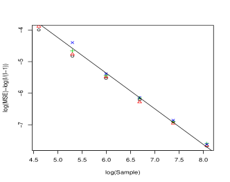
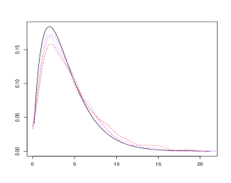
Figure 1: Example 1, Left: Plots of MSEs of $\beta$: I=2 ($\circ$), I=5($\vartriangle$), I=10($+$), I=20($\times$). The slope of the regression line between $\log(\mbox{MSE})-\log(I/(I-1))$ and $\log(\mbox{Sample})$ is -1.12615. Right: Estimated density of the scaled test Statistic $I/(I-1)nT_{n}^{1}$ for $n=100$ (long-dash), $n=200$ (dot) and $n=400$ (dot-dash) with the $\chi_{4}^{2}$ distribution (solid) when $I=2$.

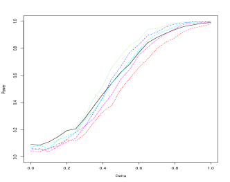
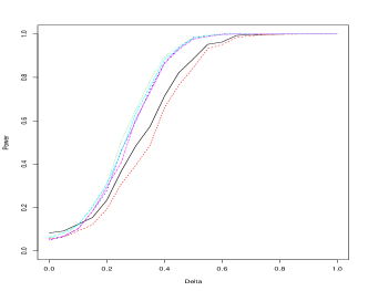
Figure 2: Power of $T_{n}^{1}$ for Example 1, Left: $n=100$, Right $n=200$. Solid line(I=2), Dot line (I=5) and Long dash line (I=10) are power curves based on scaled $\chi^{2}(4)$ distribution. Short dash line (I=2), Dot-Short dash line (I=5), Dot-long dash line (I=10) are power curves based on the bootstrap algorithm for $T_{n}^{1}$.

 Example 2.

Consider the following generalized additive model,

$$Y_{i}=X_{i}^{\top}{\beta}+g_{1}(Z_{1i})+g_{2}(Z_{2i})+g_{3}(Z_{3i})+\varepsilon_{i},\ i=1,\ldots,n$$

where parameter $\beta$ equals to $(1.5,0.3,0,0,0,0)^{\top}$. The functions $g_{1},g_{2},g_{3}$ are:

$$g_{1}(Z_{1i})=-5\sin(2Z_{1i}),\hskip 14.22636ptg_{2}(Z_{2i})=(Z_{2i})^{2}-2/3,\hskip 14.22636ptg_{3}(Z_{3i})=Z_{3i}.$$

$X_{i}$ follows a multivariate normal distribution with mean vector zero and the covariance matrix as in Example 1. The $Z$ are constructed to be highly correlated.

$$Z_{1} = X_{1}+N(0,1)$$

$$Z_{2} = Z_{1}+n^{-1/2}u_{1}$$

$$Z_{3} = Z_{1}+n^{-1/2}u_{2}$$

where $n$ is the sample size and $u_{s}$ ($s=1,2$) are $N(0,1)$ variables independent of the covariates. The correlation of $Z$ therefore goes up with sample size. Finally the error term $\varepsilon_{i}\sim N(0,1)$.

[caption=The Average Estimation Errors for Example 2 (estimated standard errors in parentheses), label= simul1, pos=h!]lrccccccccccc Method & Our Method GAM I=2 I=5 I=10 I=20 n=100 1.375(0.569) 1.305(0.482) 1.636(0.580) 2.463(0.865) 1.134 (0.454) n=200 0.741(261) 0.738(0.257) 0.876(0.317) 1.093(0.401) 0.791(0.291) n=400 0.519(0.184) 0.432(0.161) 0.473(0.165) 0.596(0.221) 0.562(0.213)

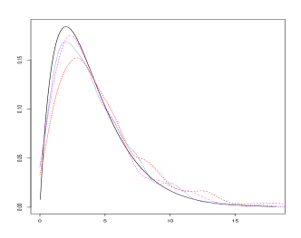
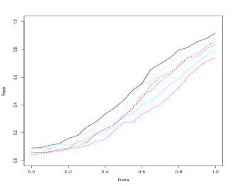
Figure 3: Example 2, Left: Estimated density of the Test Statistics $I/(I-1)nT_{n}^{1}$ for $n=100$ (long-dash) , $n=200$ (dot) and $n=400$ (dot-dash) with the $\chi_{4}^{2}$ distribution (solid) when $I=2$. Right: Power of $T_{n}^{1}$, Solid line(I=2), Dot line (I=5) and Long dash line (I=10) are power curves based on $\chi^{2}_{4}$ distribution. Short dash line (I=2), Dot-Short dash line (I=5), Dot-long dash line (I=10) are power curves based on the bootstrap algorithm for $T_{n}^{1}$.

As in Example 1, 400 simulation examples are used to evaluate the performance of the proposed estimating method. One thousand simulation examples and the same number of bootstrap samples are used to study the properties of $T_{n}^{1}$ for the same testing problem investigated in Example 1. As indicated by Table 2, as sample size increases, our proposed method outperforms the am ~packae even when $I=2$. In general, we can see that the proposed method is not sensitive to the choice of $I$ as long as it is not chosen to be too large a value relative to the sample size. Given a fixed sample size, larger $I$ will yield smaller number of subintervals and lead to coarser approximation of the nonparametric function. The empirical null distribution of $(I-1)/InT_{n}^{1}$ in comparison with $\chi^{2}_{4}$ is shown in Figure 3. It can be seen that as in Example 1, the empirical null distribution is a reasonable approximation of the asymptotical null distribution $\chi_{4}^{2}$. This is true for various values of $I$. It is also consistent with the result of Theorem 2.

Compared with the results in Example 1, additional nonparametric component increases the estimation variability for our proposed method and the method of GAM. ASE and standard errors are larger in Example 2. It also reduces the power of $T_{n}^{1}$ for the same testing problem as shown in the right graph of Figure 2. However, our proposed method is more robust to the high correlation situation as it is able to produce more efficient results than

am ~when sample size increases.
{\exm \label{example-cate} The model is
$$
Y_i = X_i^{\top}\beta+

(Z_i^d,Z_2^c)+ε_i,  i=1,…,n.

$$where$$

g(Z_i^d,Z_i^c)=(Z_i^c)^2+2Z_i^c+0.25Z_i^de^-16Z_i^c2.

$$andthetrueparameter\beta isa6\times 1vectorandequalsto(3.5,1.3,0,\cdots,0)^{\top}.X_{i},i=1,\ldots,nareindependentlygeneratedfromBernoullidistributionwithequalprobabilitybeing0or1.ThecategoricalvariableZ_{i}^{d}isaBernoullivariableindependentofX_{i}withP(Z_{i}^{d}=1)=0.7.ThevariableZ_{i}^{c}iscontinuousandsampledfromauniformdistributionon[-1,1]andindependentofX_{i}andZ_{i}^{d}.Theerrorterm\varepsilon\sim N(0,0.2^{2}).$$

For comparison purpose, we use R package p ~to estimate the bivariate fuction $g(Z_{i}^{d},Z_{i}^{c})$ nonparametrically. In addition, we also use package

am ~to
estimate a ‘‘pseudo" model with an additive nonparametric structure specified as below,
{\label{example-pseudo}
$$

(Z_i^d, Z_i^c)= δZ_i^d+ g(Z_i^c)+ε_i,  i=1,…,n.

The true nonparametric components are plotted in the left panel of Figure 4. We can see that the “pseudo” model misspecifies the nonparametric components. It will be interesting to compare the performance of the proposed method, generalized additive model and nonparametric method in terms of estimation of the parametric parameter $\bm{\beta}$.

Again, we produced 400 samples for numerical comparison. Table 3 presents the ASE and estimates of $\bm{\beta}$ under three different methods. The p ~method tries to estimate $\bbeta$ ad the bivariate function $g(Z_{1},Z_{2})$ simultaneously which involves iterative algorithm and complicated tuning parameter selections. Hence we expect the numerical performance will be compromised to some extent. As the other two simulation studies suggested, our method in general produces slightly bigger ASE than the p ~method but i a factor less than $I/(I-1)$. On the other hand our method produces more precise estimates of $\bm{\beta}$ than the nonparametric approach. It is interesting that the GAM approach outperforms the nonparametric approach even under the wrong model specification. In the left panel of Figure 4, we can see that the difference between curves $g(Z_{i}^{c},Z_{i}^{d}=0)$ and $g(Z_{i}^{c},Z_{i}^{d}=1)$ is small relative to the noise hence the more parsimonious specification of the nonparametric part to some extent improves the parametric estimation. However, under the GAM model wrong inference regard the nonparametric components will be made.

In Table 4 we compare the empirical standard deviation of $\hat{\bm{\beta}}$ (SD_m) with the one calculated under proposed sandwich formula (2.   7)(SD). It is obvious that our proposed formula provide a consistent estimate of the standard deviation of the estimate $\hat{\bm{\beta}}$.

[caption=Fitting Results of ASE and Estimation of $\bm{\beta}$ for Example 3 based on the proposed method, NP and GAM (estimated standard errors in parentheses), label= simul3, pos=h!]lrcccccccccccc Method &   Our Method NP GAM n I=2 I=5 I=10 I=20 100 ASE 0.302 (0.104) 0.298(0.091) 0.367(0.118) 0.505(0.165) 0.254 (0.091) 0.217 (0.078)   $\beta_{1}$ 3.504(0.067) 3.502(0.063) 3.506(0.076) 3.498 (0.112) 3.464 (0.058) 3.499(0.047)   $\beta_{2}$ 1.305 (0.067) 1.294(0.065) 1.302(0.086) 1.310(0.100) 1.291(0.055) 1.302 (0.047) 200 ASE 0.197(0.064) 0.163(0.052) 0.187(0.059) 0.242(0.072) 0.153 (0.052) 0.149(0.048)   $\beta_{1}$ 3.502(0.045) 3.497 (0.033) 3.498(0.042) 3.504 (0.055) 3.486 (0.032) 3.499(0.030)   $\beta_{2}$ 1.300(0.041) 1.299(0.035) 1.303(0.039) 1.297 (0.054) 1.293(0.031) 1.299(0.032) 400 ASE 0.138 (0.041)) 0.113(0.037) 0.105(0.035) 0.121(0.042) 0.102(0.032) 0.108 (0.037)   $\beta_{1}$ 3.500(0.029) 3.499(0.024) 3.500(0.022) 3.501(0.027) 3.492(0.022) 3.497 (0.021)   $\beta_{2}$ 1.303(0.031) 1.298(0.022) 1.300(0.023) 1.300(0.024) 1.300 (0.024) 1.300 (0.023)

[caption=Standard Deviations of Estimates $\hat{\beta}_{1}$ and $\hat{\beta}_{2}$ in Example 3 (estimated standard errors in parentheses), label= simul3err, pos=h!]lrccccccccccc  &   I=2 I=5 I=10 I=20 n   SD SD_m (SD_mad) SD SD_m (SD_mad) SD SD_m(SD_mad) SD SD_m(SD_mad) 100 $\beta_{1}$ 0.067 0.061(0.0088) 0.063 0.057(0.0067) 0.076 0.071(0.0073) 0.112 0.096(0.0105)   $\beta_{2}$ 0.0670.062(0.0079) 0.0650.058(0.0063) 0.086 0.071 (0.0079) 0.100 0.096(0.0112) 200 $\beta_{1}$ 0.045 0.041(0.0037) 0.033 0.035(0.0021) 0.042 0.037(0.0024) 0.055 0.048(0.0046)   $\beta_{2}$ 0.041 0.041(0.0038) 0.035 0.034(0.0022) 0.039 0.037(0.0024) 0.054 0.048(0.0044) 400 $\beta_{1}$ 0.029 0.028(0.0018) 0.024 0.023(0.0010) 0.022 0.023(0.0009) 0.027 0.025(0.0010)   $\beta_{2}$ 0.031 0.028(0.0018) 0.022 0.023(0.0011) 0.023 0.023(0.0009) 0.024 0.025(0.0010)

Next we test the equivalence of the two nonparametric components associated with $Z^{d}=0,1$,

$$\begin{split}&H_{0}^{2}:g(Z^{c},Z^{d}=0)=g(Z^{c},Z^{d}=1),\\ &H_{1}^{2}:g(Z^{c},Z^{d}=0)\neq g(Z^{c},Z^{d}=1)\end{split}$$

In this simulation example, $g(Z_{i}^{c},Z_{i}^{d}=0)=(Z_{i})^{c2}+2Z_{i}^{c}$ and $g(Z_{i}^{c},Z_{i}^{d}=1)=(Z_{i})^{c2}+2Z_{i}^{c}+\delta\exp(-16(Z_{i}^{c2}))$. To explore the relationship between effect size and power of our proposed test statistic $T_{n}^{2}$, we let the value of $\delta$ change from 0 to 0.25.

To calculate $T_{n}^{2}$, we first get the estimate of $\bm{\beta}$, $\hat{\bm{\beta}}$ using formula (2.5), then remove it from the model,

$$Y^{\ast}_{i}=g(Z_{i}^{c},Z_{i}^{d})+\varepsilon^{\ast}_{i},\quad i=1,\ldots,n$$

where $Y_{i}^{\ast}=Y_{i}-X_{i}\hat{\bm{\beta}}$ and $\varepsilon_{i}^{\ast}=\varepsilon_{i}+X_{i}\bm{\beta}-X_{i}\hat{\bm{\beta}}$. Next we use R package ocfit ~to seect a bandwidth $h$ and in fact use $0.8h$ to get slightly under-smoothed estimates of $\hat{g}(Z_{i}^{c},Z_{i}^{d}=0)$ and $\hat{g}(Z_{i}^{c},Z_{i}^{d}=1)$ and their variance estimates. The test statistic $T_{n}^{2}$ is calculated by plugging these estimators into formula (3.   16). The $p$-values associated with $T_{n}^{2}$ are calculated using the bootstrap procedure suggested in Section 3. One thousand bootstrap samples are used to approximate the null distribution of $T_{n}^{2}$. This procedure is repeated 400 times to calculate the power of the test statistic under the alternative models defined by various $\delta$ values from 0 to 0.25.

The empirical distribution and bootstrapped distribution of $T_{n}^{2}$ under null hypothesis when $\delta=0$ and the bootstrapped null distribution approximation under alternative hypothesis when $\delta=0.083,0.167,0.25$ at sample size $n=200$ and $I=5$ are shown in the middle graph of Figure 4. We can see that the bootstrapped distributions under different alternative models provide fairly good approximations to the real null hypothesis distribution of our proposed test statistics. It suggests that the asymptotical null distribution of the proposed test statistics for our two population nonparametric testing problem should be a model free test statistic. In the right panel of Figure 4, the power curves of $T_{n}^{2}$ under various $\delta$ values and different sample sizes are shown. The estimates of $\bm{\beta}$ have little impact on the power curves and such impact is only through sample size. As a two-population nonparametric test, it is not too surprising to see that the power of this test is relatively low for small sample size. But as the sample size doubles, the power function picks up quickly even for small effect size when $\delta=0.1$.

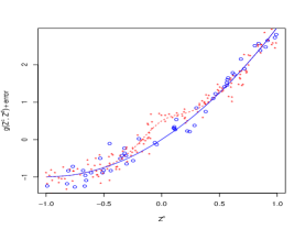
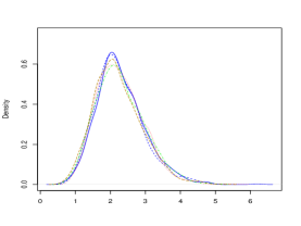
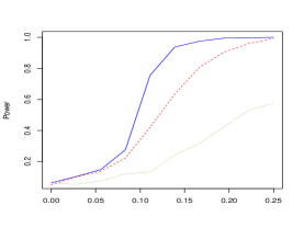
Figure 4: Example 3, Left: Scatterplot of $g(Z^{c},Z^{d})+$error vs $Z_{2}$ overlaid by solid-blue line: $g(Z^{c},Z^{d}=0)$ and dash-red line: $g(Z^{c},Z_{d}=1)$. Middle: Estimated density of the empirical and bootstrap null distribution of $nT_{n}^{2}$ for $n=200$ and $I=5$: solid blue line ($\delta=0$) is the empirical null distribution. Dash-blue line ($\delta=0$), dot-red line ($\delta=0.083$), dot-dash green line ($\delta=0.167$) and long-dash dark golden red line ($\delta=0.25$) are bootstrapped estimation of null distribution. Right: the power function evaluated at $I=5$ and different $\delta$ values with different sample sizes $n=100$ (dot line), $n=200$ (dash line) and $n=400$ (solid line).

5. Real data application: correlates of birth weight

Low birth weight is an important biological indicator since it is associated with both birth defects and infant mortality. A woman’s physical condition and behavior during pregnancy can greatly affect the birth weight of the newborn. In this section, we apply our proposed methods to a classic example studying the determinants of birth weights (Hosmer and Lemeshow, 2000). This dataset is part of a larger study conducted at Bay State Medical Center in Springfield, Massachusetts. The dataset contains variables (see below) that are believed to be associated with low birth weight in the obstetrical literatures. The goal of the analysis is to determine whether these variables are risk factors in the clinical population being served by Bay State Medical Center.

• MOTH_AGE: Mother’s age (years)

• MOTH_WT: Mother’s weight (pounds)

• Black: Mother’s race being black (’White’ is the reference group)

• Other: Mother’s race being other than black or white

• SMOKE: Mother’s smoking status (1=Yes, 0=No)

• PRETERM: Any history of premature labor (1=Yes, 0=No)

• HYPER: History of hypertension (1=Yes, 0=No)

• URIN_IRR: History of urinary irritation (1=Yes, 0=No)

• PHYS_VIS: Number of physician visits

• BIRTH_WT Birth weight of new born (grams)

First we analyze this data set using a linear regression model to estimate the relationship between various factors and birth weight. Shown in Table 5 (OLS-1 model), mother’s race (Black vs White, Other vs White), history of pregnancy hypertension and history of urinary irritation have significantly negative impact on birth weights of newborns, while mother’s weight is positively related to birth weight. Perhaps surprisingly, mother’s age is not a significant predictor of baby’s birth weight(p-value=0.30). To check the linearity assumption with respect to the two continuous predictors, mother’s age and weight, standardized residual plot against each of them is examined. Figure 5a shows that linearity is an adequate assumption for mother’s weight and this relationship is not different between smokers and nonsmokers. But the residual diagnostics (graph not shown) indicate that the relationship between mother’s age and birth weight is not linear and the relationship could potentially vary by mother’s smoking status.

Then we expand the analysis to 1) a linear regression with interaction term between age and smoking (the OLS-2 model), and 2) a generalized additive model (GAM) that specifies a nonparametric term with respect to mother’s age. Under the OLS-2 model, the baseline age effect is insignificant. Although the interaction term improves the model fit slightly, it is deemed insignificant (p-value=0.12). Under the GAM model, the nonparametric term of age is also tested insignificant (p-value=0.56). The conclusions about the effects of other variables on birth weights are similar compared to the OLS-1 model.

[caption = Estimated effects of correlates of birth weight and their standard errors, label=real-data, pos=!h] cccccc & OLS-1 OLS-2 GAM PL Intercept 3026.9(308.2) 2741.9(357.0) 3044.2(309.0) 2482.0(388.2) MOTH_WT 4.6(1.7) 4.5(1.7) 4.5(1.7) 5.6(2.0) Black -482.2(146.8) -431.5(149.7) -480.1(147.4) -295.2(175.2) Other -327.5(112.6) -302.2(113.3) -320.1(112.9) -203.6(132.8) PRETERM -179.5(133.8) -169.8(133.4) -166.4(134.2) -220.0(153.5) HYPER -584.4(197.6) -588.4(196.8) -582.2(198.1) -651.7(232.2) URIN_IRR -492.3(134.6) -526.1(135.8)-508.2(134.9) -510.2(153.6) PHYS_VIS -7.0(45.4) -0.7(45.4) -12.2(45.5) -14.7(52.8) MOTH_AGE -10.4(9.9) 1.8(12.6) —(—) —(—) SMOKE -312.5(104.5) 402.1(468.5) -321.3(104.7) —(—) MOTH_AGE $\times$ SMOKE —(—) -30.6(19.6) —(—) —(—) $R^{2}$ 0.251 0.261 0.255 0.391

To model the nonlinear relationship between age and birth weight as well as its interaction with mother’s smoking status, we further fit this data to a partially linear model with a bivariate nonparametric components, specified as,

$$\begin{array}[]{rll}\mbox{BirthWT}&=&\beta_{0}+\beta_{1}\mbox{MOTH\_WT}+\beta_{2}\mbox{Black}+\beta_{3}\mbox{Other}+\beta_{4}\mbox{PRETERM}+\beta_{5}\mbox{HYPER}\\ &&+\beta_{6}\mbox{URIN\_IRR}+\beta_{7}\mbox{PHYS\_VIS}+g(\mathrm{MOTH\_AGE},\mathrm{SMOKE})+\varepsilon.\end{array}$$ (5.   1)

We then fit this model using the method proposed in Section 2.3. Since mother’s age is recorded by a series of discrete values from 14 to 36 years, we first partition the support of $g(\mbox{MOTH\_AGE},\mbox{SMOKE})$ according to mother’s smoking status, then estimate the nonparametric response curve for each group at every distinct age using available sample points (instead of using fixed cell size). The parameter estimates of the parametric components with standard errors are given in the last column of Table 5.

Given the parametric components, we re-estimate $g(\mbox{MOTH\_AGE},\mbox{SMOKE})$ using the local polynomial regression methods via

ocfit. The fitted curves
(after removing the parametric components) are shown in the right pane

of Figure 5. This figure reveals that the response curves between age and birth weight are quite different for smoking and nonsmoking mothers. We can see that among non-smoking mothers, age is not particularly associated with birth weight. However, for smoking mothers, the birth weight decreases quite dramatically as mother’s age increases. The gap is as wide as over 400 grams of birth weight between nonsmoking and smoking mothers who are 30 years and older. Similar as in the simulation studies, in the local polynomial regression (

ocfit), a quadratic term is used
and the optima

bandwidth is chosen via generalized cross validation.

We also conduct the following one-sided nonparametric test to compare the two response curves between smokers and nonsmokers,

$$\begin{split}&H_{0}^{2}:g(\mbox{MOTH\_AGE},\mbox{Smoke})=g(\mbox{MOTH\_AGE},\mbox{Nonsmoke}),\mbox{\,\, almost everywhere}\\ &H_{1}^{2}:g(\mbox{MOTH\_AGE},\mbox{Smoke})<g(\mbox{MOTH\_AGE},\mbox{Nonsmoke}),\mbox{\,\, on a set with positive measure}.\end{split}$$ (5.   2)

Based on (3.16), the test statistic $T_{n}^{2}$ for the above test is 3.36, and the bootstrap p-value is 0.029, suggesting that the response curve of age among smokers is lower than that of non-smokers. Taking this result and Figure 5b, we can see that the PL model provides a better specification for the relationship between mother’s age, smoking status and birth weight.

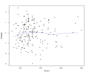
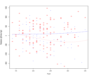
Figure 5: Correlates of birth weight: The left graph plots the residuals (OLS-2) vs mother’s weight. The dotted red and dashed blue lines are the lowess fits for smoking mothers and non-smoking mothers, respectively. The right graph plots estimated regression function $g(\mbox{Age},\mbox{Smoke})$ removing the effects of other covariates under the partial consistency PL model. The dotted red and dashed blues are the (lcofit) nonparametric estimates of response curves for smoking and non-smoking mothers, respectively.

The estimates of the parameter components of the PL model also exhibit some interesting changes compared with other models. We can see the racial gap in birth weight narrows. Controlling other factors, on average babies born to Black mothers are 295 grams lighter than those born to White mothers. This difference is much smaller compared to the previous models. In addition, based on the test statistic defined in (3.13), the effect of ”Black” now is only marginally significant (p-value=0.1) and the effect of ”Other” becomes insignificant (p-value=0.147). The effect sizes and significance values of other covariates remain about the same.

6. Discussion

In this paper, based on the concept of partial consistency, we proposed a simple estimation method to partially linear regression model. The nonparametric component of the model is transformed into a set of artificially created nuisance or incidental parameters. Though these nuisance parameters cannot be estimated consistently, the parametric components of the partially linear model can be estimated consistently and almost efficiently under this configuration. As long as the sample size is reasonably large, the number of the nuisance parameters used is not too important. The estimation results have been shown to be fairly stable under various “coarseness” of the approximation. The statistical inference with respect to the parametric components via profile likelihood ratio test is also efficient. Generally speaking, the proposed simple estimation method for the partially linear regression model has two advantages that are worth noting. First, it greatly simplifies the computation burden in model estimation with little loss of efficiency. Second, it can be used to reduce the model bias by considering interaction between categorial predictor and continuous predictor, or between two continuous predictors in the nonparametric component of the model.

Though the partially linear regression model is a simple semiparameric model, the results have offered us more insights about the “bias-efficiency” tradeoff in semiparametric model estimations: when estimating the nonparametric components, pursing further bias reduction can increase the variance of nonparametric estimation, but it has little effect on the estimation of the parametric components of the model, and the efficient loss in the parametric part is small. Comparing to a much eased computational burden, such loss in efficiency in the parametric part can be negligible. Our study raised an interesting problem in semiparametric estimation: how to balance between the computation burden and the efficiency of the estimators while minimizing model bias. Our results can be generalized to estimate more broadly defined semiparametric models utilizing the partial consistency properties to fully exploit the information in the data.

7. Appendix: assumptions and proofs

We need the following conditions to prove our theoretical results:

1. $E|\varepsilon|^{4}<\infty$ and $E\|X\|^{4}<\infty$.
   

2. The support of the continuous component of $Z$ is bounded.
   

3. The functions $g(z^{d},z^{c})$, $\mathop{\mbox{\sf E}}(X|Z^{d}=z^{d},Z^{c}=z^{c})$, the density function of $Z$, and their corresponding second derivatives with respect to $z^{c}$ are all bounded.
   

4. $\Sigma$ is nonsingular.
   

5. In presence of discrete covariate in $Z$, assume that for any category, the number of samples lies in this category is large enough and of order $n$.

For simplicity of presentation, we only discuss the case of $Z=Z^{c}$ and prove Theorem 1. When $Z$ is of $2$-dimension, we mainly consider that one component of $Z$ is discrete or both components in $Z$ are highly correlated. For the former case, according to condition (e) it can be concluded that each category has a sample size of order $n$. So categories do not affect the following proof which leads to the results of Corollary 1 . For the latter case, assumption (2.   10) implies that the following proof can be easily generalized to obtain Corollary 2. The proofs for both Corollary 1 and Corollary 2 are therefore omitted here.

Proof of Theorem 1. First, based on standard operations in least squares estimation, we can obtain the decomposition $\sqrt{n}(\hat{\beta}-\beta)=R_{1}+R_{2}$, where

$$\begin{split}R_{1}&=\Big{\{}\frac{1}{n}\sum\limits_{j=1}^{J}\sum\limits_{i=1}^{I}\{X_{(j-1)I+i}-\frac{1}{I}\sum\limits_{i=1}^{I}X_{(j-1)I+i}\}^{T}\{X_{(j-1)I+i}-\frac{1}{I}\sum\limits_{i=1}^{I}X_{(j-1)I+i}\}\Big{\}}^{-1}\\ &\hskip 2.84544pt\times\Big{\{}\frac{1}{\sqrt{n}}\sum\limits_{j=1}^{J}\sum\limits_{j=1}^{J}\{X_{(j-1)I+i}-\frac{1}{I}\sum\limits_{i=1}^{I}X_{(j-1)I+i}\}^{T}\{g(Z_{(j-1)I+i})-\frac{1}{I}\sum\limits_{i=1}^{I}g(Z_{(j-1)I+i})\}\Big{\}}\\ &\equiv{R_{1}^{N}}/{R_{1}^{D}}\end{split}$$ (A.1)

and

$$\begin{split}R_{2}&=\Big{\{}\frac{1}{n}\sum\limits_{j=1}^{J}\sum\limits_{i=1}^{I}\{X_{(j-1)I+i}-\frac{1}{I}\sum\limits_{i=1}^{I}X_{(j-1)I+i}\}^{T}\{X_{(j-1)I+i}-\frac{1}{I}\sum\limits_{i=1}^{I}X_{(j-1)I+i}\}\Big{\}}^{-1}\\ &\hskip 2.84544pt\times\Big{\{}\frac{1}{\sqrt{n}}\sum\limits_{j=1}^{J}\sum\limits_{j=1}^{J}\{X_{(j-1)I+i}-\frac{1}{I}\sum\limits_{i=1}^{I}X_{(j-1)I+i}\}^{T}\{\varepsilon_{(j-1)I+i}-\frac{1}{I}\sum\limits_{i=1}^{I}\varepsilon_{(j-1)I+i}\}\Big{\}}\\ &\equiv{R_{2}^{N}}/{R_{2}^{D}}\\ \end{split}$$ (A.2)

Hereby we will show that the term $R_{1}$ converges to zero in probability as $n\rightarrow\infty$ and the asymptotic distribution of $R_{2}$ is multivariate normal with zero mean vector and covariance matrix given in (2.   11).

According to the form of $R_{1}$, we need to first analyze the numerator $R_{1}^{N}$ and the denominator $R_{1}^{D}$ respectively. Let $\mathcal{F}_{n}=\sigma\{Z_{1},Z_{2},\cdots,Z_{n}\}$ and observe that conditionally on $\mathcal{F}_{n}$, $X_{(j-1)I+i}$ are independent of each other. The following is a sketch.

We first analyze $R_{1}^{N}$. Denote $\mathop{\mbox{\sf E}}(X|Z=z)$ by $m(z)$ and $X-m(Z)$ by $e$, then

$$\begin{split}R_{1}^{N}=&\frac{1}{\sqrt{n}}\sum\limits_{j=1}^{J}\sum\limits_{i=1}^{I}\{m(Z_{(j-1)I+i})-\frac{1}{I}\sum\limits_{i=1}^{I}m(Z_{(j-1)I+i})\}\{g(Z_{(j-1)I+i})-\frac{1}{I}\sum\limits_{i=1}^{I}g(Z_{(j-1)I+i})\}\\ &+\frac{1}{\sqrt{n}}\sum\limits_{j=1}^{J}\sum\limits_{i=1}^{I}\{e_{(j-1)I+i}-\frac{1}{I}\sum\limits_{i=1}^{I}e_{(j-1)I+i}\}\{g(Z_{(j-1)I+i})-\frac{1}{I}\sum\limits_{i=1}^{I}g(Z_{(j-1)I+i})\}\\ &=R_{1}^{N(1)}+R_{1}^{N(2)}.\end{split}$$ (A.3)

Notice that $R_{1}^{N(1)}$ can be expressed using the following summations,

$$\begin{split}&R_{1}^{N(1)}=\frac{1}{\sqrt{n}I^{2}}\sum\limits_{j=1}^{J}\sum\limits_{i=1}^{I}\sum\limits_{l=1}^{I}\sum\limits_{k=1}^{I}\{m(Z_{(j-1)I+i})-m(Z_{(j-1)I+l})\}\{g(Z_{(j-1)I+i})-g(Z_{(j-1)I+k})\}\\ \end{split}$$

Parallel to the proof of Hsing and Carroll (1992) and Zhu and Ng (1995), we can show that

$$\begin{split}R_{1}^{N(1)}\leq&\frac{1}{\sqrt{n}I^{2}}\sqrt{\sum\limits_{j=1}^{J}\sum\limits_{i=1}^{I}\sum\limits_{l=1}^{I}\sum\limits_{k=1}^{I}\|m(Z_{(j-1)I+i})-m(Z_{(j-1)I+l})\|^{2}}\\ &\hskip 14.22636pt\times\sqrt{\sum\limits_{j=1}^{J}\sum\limits_{i=1}^{I}\sum\limits_{l=1}^{I}\sum\limits_{k=1}^{I}|g(Z_{(j-1)I+i})-g(Z_{(j-1)I+k})|^{2}}\\ =&O_{P}(n^{-1/2}I^{-2}n^{\delta})=o_{P}(1).\end{split}$$

Here $\delta$ is a arbitrarily small positive constant. Let $\Omega_{j}$ denote the sample set lying in the $j$th partition with $1\leq j\leq J$. The last equality obtained from the fact that, under condition (c), $m(\cdot)$ and $g(\cdot)$ have a total variation of order $\delta$,

$$\begin{split}&\lim\limits_{n\rightarrow\infty}\frac{1}{n^{\delta}}\sup\limits_{\{\Omega_{j},1\leq j\leq J\}}\sum\limits_{i=1}^{I-1}\|m(Z_{(j-1)I+i})-m(Z_{(j-1)I+(i+1)})\|=0,\\ &\lim\limits_{n\rightarrow\infty}\frac{1}{n^{\delta}}\sup\limits_{\{\Omega_{j},1\leq j\leq J\}}\sum\limits_{i=1}^{I-1}|g(Z_{(j-1)I+i})-g(Z_{(j-1)I+(i+1)})|=0.\end{split}$$

Next we consider $R_{1}^{N(2)}$. Let $\bar{e}_{(n)}$ and $\bar{e}_{1}$ be the largest and smallest of the corresponding $e_{i}$’s, respectively. It is clear that

$$\begin{split}R_{1}^{N(2)}\leq&\frac{\bar{e}_{(n)}-\bar{e}_{1}}{\sqrt{n}I}\sum\limits_{j=1}^{J}\sum\limits_{i=1}^{I}\sum\limits_{l=1}^{I}|g(Z_{(j-1)I+i})-g(Z_{(j-1)I+l})|\\ =&2\frac{\bar{e}_{(n)}-\bar{e}_{1}}{\sqrt{n}I}\sum\limits_{j=1}^{J}\sum\limits_{1\leq i<l\leq I}|g(Z_{(j-1)I+i})-g(Z_{(j-1)I+l})|\end{split}$$

The above argument leads to that

$$\begin{split}R_{1}^{N(2)}\leq&2\frac{\bar{e}_{(n)}-\bar{e}_{1}}{\sqrt{n}I}\sum\limits_{i=1}^{I}\sum\limits_{l=1}^{I}\sum\limits_{j=1}^{n-1}|g(Z_{(j+1)})-g(Z_{(j)})|\\ \leq&2I\frac{\bar{e}_{(n)}-\bar{e}_{1}}{\sqrt{n}}\sum\limits_{j=1}^{n-1}|g(Z_{(j+1)})-g(Z_{(j)})|.\end{split}$$

Applying Lemma A.1 of Hsing and Carroll (1992), we obtain

$$n^{-1/4}|\bar{e}_{(n)}-\bar{e}_{1}|\stackrel{{\scriptstyle P}}{{\longrightarrow}}0.$$

Note the fact that total variation of $g(\cdot)$ is of order $n^{\delta}$, we have $R_{1}^{N(2)}=o_{P}(1)$. Combining the results about $R_{1}^{N(1)}$ and $R_{1}^{N(2)}$, the proof for $R_{1}^{N}$ is completed.

Next consider $R_{1}^{D}$ and $R_{2}^{D}$. Since $R_{1}^{D}=R_{2}^{D}$, we only need to show the case of $R_{1}^{D}$. The expectation of $R_{1}^{D}$ is calculated as follows.

$$\begin{split}\mathop{\mbox{\sf E}}(R_{1}^{D})=&\mathop{\mbox{\sf E}}(XX^{\top})-\frac{1}{nI}\sum\limits_{j=1}^{J}\sum\limits_{i=1}^{I}\sum\limits_{l=1}^{I}E\{X_{(j-1)I+i}X_{(j-1)I+l}\}\\ =&\mathop{\mbox{\sf E}}(XX^{\top})-\frac{1}{nI}\sum\limits_{j=1}^{J}\sum\limits_{i=1}^{I}E\{X_{(j-1)I+i}X_{(j-1)I+i}\}-\frac{1}{nI}\sum\limits_{j=1}^{J}\sum\limits_{i\neq l}E\{X_{(j-1)I+i}X_{(j-1)I+l}\}\\ =&(1-\frac{1}{I})\mathop{\mbox{\sf E}}(XX^{\top})-\frac{1}{nI}\sum\limits_{j=1}^{J}\sum\limits_{i\neq l}E\Big{[}E\{X_{(j-1)I+i}X_{(j-1)I+l}|\mathcal{F}_{n}\}\Big{]}\\ \end{split}$$

Under the assumption that conditionally on $\mathcal{F}_{n}$, $X_{(j-1)I+i}$ are independent of each other, we can obtain that $E\{X_{(j-1)I+i}X_{(j-1)I+l}|\mathcal{F}_{n}\}=m(Z_{(j-1)I+i})m(Z_{(j-1)I+l})$. This, together with the above analysis, gives

$$\begin{split}\mathop{\mbox{\sf E}}(R_{1}^{D})=&(1-\frac{1}{I})\mathop{\mbox{\sf E}}(XX^{\top})-\frac{I-1}{nI}\sum\limits_{j=1}^{J}\sum\limits_{i=l}^{I}E\Big{[}m(Z_{(j-1)I+i})m(Z_{(j-1)I+i})\Big{]}\\ &-\frac{1}{nI}\sum\limits_{j=1}^{J}\sum\limits_{i\neq l}E\Big{[}m(Z_{(j-1)I+i})\{m(Z_{(j-1)I+l})-m(Z_{(j-1)I+i})\}\Big{]}\\ =&(1-\frac{1}{I})\mathop{\mbox{\sf E}}(XX^{\top})-\frac{I-1}{nI}\sum\limits_{j=1}^{J}\sum\limits_{i=l}^{I}E\Big{[}m(Z_{(j-1)I+i})m(Z_{(j-1)I+i})\Big{]}+o(1)\\ =&(1-\frac{1}{I})E\Big{[}\{X-\mathop{\mbox{\sf E}}(X|Z)\}\{X-\mathop{\mbox{\sf E}}(X|Z)\}^{\top}\Big{]}+o(1).\end{split}$$

The term of order $o(1)$ is obtained following a similar argument of Theorem 2.3 of Hsing and Carroll (1992). This completes the proof for $R_{1}$.

We now deal with the term $R_{2}$. Observe that given $\{(X_{i},Z_{i}),i=1,\cdots,n\}$, each term of $\{\varepsilon_{(j-1)I+i}-\frac{1}{J}\sum\limits_{j=1}^{J}\varepsilon_{(j-1)I+i}\}$ has mean zero and is independent of each other. Thus $R_{2}$ is asymptotically normal with mean zero. We will show that the limiting variance of $R_{2}$ is equal to the covariance matrix given in (2.   11). That is,

$$\begin{split}\mbox{Var}(R_{2}|\{X_{i},Z_{i}\})=&(R_{2}^{D})^{-1}\mbox{Var}(R_{2}^{N}|\{X_{i},Z_{i}\})(R_{2}^{D})^{-1}\\ =&\{\mathop{\mbox{\sf E}}(R_{2}^{D})\}^{-1}\mathop{\mbox{\sf E}}\{\mbox{Var}(R_{2}^{N}|\{X_{i},Z_{i}\})\}\{\mathop{\mbox{\sf E}}(R_{2}^{D})\}^{-1}+o_{P}(1)\end{split}$$

and

$$\begin{split}\mbox{Var}(R_{2}^{N}|\{X_{i},Z_{i}\})=&\frac{1}{n}\sum\limits_{j=1}^{J}\sum\limits_{i=1}^{I}\{X_{(j-1)I+i}-\frac{1}{I}\sum\limits_{i=1}^{I}X_{(j-1)I+i}\}\{X_{(j-1)I+i}-\frac{1}{I}\sum\limits_{i=1}^{I}X_{(j-1)I+i}\}^{\top}\\ &\hskip 28.45274pt\times\mathop{\mbox{\sf E}}\Big{[}\{\varepsilon_{(j-1)I+i}-\frac{1}{I}\sum\limits_{i=1}^{I}\varepsilon_{(j-1)I+i}\}^{2}\Big{|}\{X_{i},Z_{i}\}\Big{]}\\ =&\frac{\sigma^{2}}{n}\sum\limits_{j=1}^{J}\sum\limits_{i=1}^{I}\{X_{(j-1)I+i}-\frac{1}{I}\sum\limits_{i=1}^{I}X_{(j-1)I+i}\}\{X_{(j-1)I+i}-\frac{1}{I}\sum\limits_{i=1}^{I}X_{(j-1)I+i}\}^{\top}\\ \stackrel{{\scriptstyle P}}{{\longrightarrow}}&\sigma^{2}(1-\frac{1}{I})\mathop{\mbox{\sf E}}\Big{[}\{X-\mathop{\mbox{\sf E}}(X|Z)\}\{X-\mathop{\mbox{\sf E}}(X|Z)\}^{\top}\Big{]}.\end{split}$$

Combining the last two equations, we complete the proof of Theorem 1. $\Box$

Proof of Theorem 2. First we show that $\mbox{RSS}_{1}=\sigma^{2}\{1+o_{P}(1)\}$. By (2.   5),

$$\begin{split}\mbox{RSS}_{1}&=\frac{1}{n}\sum\limits_{j=1}^{J}\sum\limits_{i=1}^{I}\{Y_{(j-1)I+i}-\hat{\alpha}_{j1}-X_{(j-1)I+i}\hat{\bm{\beta}}_{1}\}^{2}\\ &=\frac{1}{n}\sum\limits_{j=1}^{J}\sum\limits_{i=1}^{I}\Big{[}\{X_{(j-1)I+i}-\frac{1}{I}\sum\limits_{i=1}^{I}X_{(j-1)I+i}\}(\bm{\beta}-\hat{\bm{\beta}}_{1})\\ &\hskip 71.13188pt+\{g(Z_{(j-1)I+i})-\frac{1}{I}\sum\limits_{i=1}^{I}g(Z_{(j-1)I+i})\}\\ &\hskip 71.13188pt+\{\varepsilon_{(j-1)I+i}-\frac{1}{I}\sum\limits_{i=1}^{I}\varepsilon_{(j-1)I+i}\}\Big{]}^{2}\\ &=I_{1}+I_{2}+I_{3}+I_{4}+I_{5}+I_{6},\end{split}$$

where

$$\begin{split}&I_{1}=\frac{1}{n}\sum\limits_{j=1}^{J}\sum\limits_{i=1}^{I}\{\varepsilon_{(j-1)I+i}-\frac{1}{I}\sum\limits_{i=1}^{I}\varepsilon_{(j-1)I+i}\}^{2}\\ &I_{2}=\frac{1}{n}\sum\limits_{j=1}^{J}\sum\limits_{i=1}^{I}[\{X_{(j-1)I+i}-\frac{1}{I}\sum\limits_{i=1}^{I}X_{(j-1)I+i}\}(\bm{\beta}-\hat{\bm{\beta}}_{1})]^{2}\\ &I_{3}=\frac{1}{n}\sum\limits_{j=1}^{J}\sum\limits_{i=1}^{I}\{g(Z_{(j-1)I+i})-\frac{1}{I}\sum\limits_{i=1}^{I}g(Z_{(j-1)I+i})\}^{2}\\ &I_{4}=\frac{2}{n}\sum\limits_{j=1}^{J}\sum\limits_{i=1}^{I}\{\varepsilon_{(j-1)I+i}-\frac{1}{I}\sum\limits_{i=1}^{I}\varepsilon_{(j-1)I+i}\}\{g(Z_{(j-1)I+i})-\frac{1}{I}\sum\limits_{i=1}^{I}g(Z_{(j-1)I+i})\}\\ &I_{5}=\frac{2}{n}\sum\limits_{j=1}^{J}\sum\limits_{i=1}^{I}\{X_{(j-1)I+i}-\frac{1}{I}\sum\limits_{i=1}^{I}X_{(j-1)I+i}\}(\bm{\beta}-\hat{\bm{\beta}}_{1})\{g(Z_{(j-1)I+i})-\frac{1}{I}\sum\limits_{i=1}^{I}g(Z_{(j-1)I+i})\}\\ &I_{6}=\frac{2}{n}\sum\limits_{j=1}^{J}\sum\limits_{i=1}^{I}\{X_{(j-1)I+i}-\frac{1}{I}\sum\limits_{i=1}^{I}X_{(j-1)I+i}\}(\bm{\beta}-\hat{\bm{\beta}}_{1})\{\varepsilon_{(j-1)I+i}-\frac{1}{I}\sum\limits_{i=1}^{I}\varepsilon_{(j-1)I+i}\}\end{split}$$

Using the same arguments when analyzing $R_{1}$ and $R_{2}$, it can be shown that

$$\begin{split}&I_{1}=\frac{I-1}{I}\sigma^{2}\{1+o_{P}(1)\},\hskip 28.45274ptI_{2}=O_{P}(n^{-1}),\hskip 28.45274ptI_{3}=o_{P}(n^{-1/2}),\\ &I_{4}=o_{P}(n^{-1/4}),\hskip 28.45274ptI_{5}=o_{P}(n^{-3/4}),\hskip 28.45274ptI_{6}=o_{P}(n^{-1/2}).\end{split}$$

Similarly, $\mbox{RSS}_{0}$ can be decomposed as

$$\begin{split}\mbox{RSS}_{0}&=\frac{1}{n}\sum\limits_{j=1}^{J}\sum\limits_{i=1}^{I}\{Y_{(j-1)I+i}-\hat{\alpha}_{j0}-X_{(j-1)I+i}\hat{\bm{\beta}}_{0}\}^{2}\\ &=\frac{1}{n}\sum\limits_{j=1}^{J}\sum\limits_{i=1}^{I}\Big{[}\{Y_{(j-1)I+i}-\hat{\alpha}_{j1}-X_{(j-1)I+i}\hat{\bm{\beta}}_{1}\}\\ &\hskip 56.9055pt+\{X_{(j-1)I+i}-\frac{1}{I}\sum\limits_{i=1}^{I}X_{(j-1)I+i}\}(\hat{\bm{\beta}}_{1}-\hat{\bm{\beta}}_{0})\Big{]}^{2}\\ &=\mbox{RSS}_{1}+J_{1}+J_{2},\end{split}$$

with

$$\begin{split}&J_{1}=\frac{1}{n}\sum\limits_{j=1}^{J}\sum\limits_{i=1}^{I}\Big{[}\{X_{(j-1)I+i}-\frac{1}{I}\sum\limits_{i=1}^{I}X_{(j-1)I+i}\}(\hat{\bm{\beta}}_{1}-\hat{\bm{\beta}}_{0})\Big{]}^{2}\\ &J_{2}=\frac{2}{n}\sum\limits_{j=1}^{J}\sum\limits_{i=1}^{I}\{Y_{(j-1)I+i}-\hat{\alpha}_{j1}-X_{(j-1)I+i}\hat{\bm{\beta}}_{1}\}\{X_{(j-1)I+i}-\frac{1}{I}\sum\limits_{i=1}^{I}X_{(j-1)I+i}\}(\hat{\bm{\beta}}_{1}-\hat{\bm{\beta}}_{0}).\end{split}$$

From the proof of Theorem 1, it holds that $\frac{1}{n}\sum\limits_{j=1}^{J}\sum\limits_{i=1}^{I}\{X_{(j-1)I+i}-\frac{1}{I}\sum\limits_{i=1}^{I}X_{(j-1)I+i}\}\{X_{(j-1)I+i}-\frac{1}{I}\sum\limits_{i=1}^{I}X_{(j-1)I+i}\}^{\top}\stackrel{{\scriptstyle P}}{{\longrightarrow}}\frac{I-1}{I}\Sigma$. Furthermore, the estimators for $\bm{\beta}$ under the null and alternative hypotheses then have the following relation

$$\hat{\bm{\beta}}_{0}=\hat{\bm{\beta}}_{1}-\Sigma^{-1}A^{\top}\{A\Sigma^{-1}A^{\top}\}^{-1}A\hat{\bm{\beta}}_{1}+o_{P}(\hat{\bm{\beta}}_{1}).$$

$J_{1}$ can then be written as

$$J_{1}=\frac{I-1}{I}\hat{\bm{\beta}}_{1}^{\top}A^{\top}\{A\Sigma^{-1}A^{\top}\}^{-1}A\hat{\bm{\beta}}_{1}+o_{P}(\hat{\bm{\beta}}_{1}).$$

This, together with the asymptotic normality of $\hat{\bm{\beta}}_{1}$ in Theorem 1 implies that under the null hypothesis $A\hat{\bm{\beta}}_{1}\stackrel{{\scriptstyle\mathcal{L}}}{{\longrightarrow}}N(0,\sigma^{2}\frac{I-1}{I}A\Sigma^{-1}A^{\top})$, we have $nJ_{1}\stackrel{{\scriptstyle\mathcal{L}}}{{\longrightarrow}}\sigma^{2}\chi^{2}_{k}.$ By some calculation, it can be shown that $J_{2}=0$. Thus,

$$n(\mbox{RSS}_{0}-\mbox{RSS}_{1})\stackrel{{\scriptstyle\mathcal{L}}}{{\longrightarrow}}\sigma^{2}\chi^{2}_{k}.$$

Then by Slutsky theorem,

$$nT_{n}^{1}=n\frac{\mbox{RSS}_{0}-\mbox{RSS}_{1}}{\mbox{RSS}_{1}}\stackrel{{\scriptstyle\mathcal{L}}}{{\longrightarrow}}\frac{I}{I-1}\chi^{2}_{k}.\quad\quad\Box$$

References

- Andrews (1994) Andrews, D. W. K. (1994). Asymptotic for semiparametric econometric models via stochastic equicontinuity. Econometrica, 62 43–72.
- Chen (1988) Chen, H. (1988). Convergence rates for parametric components. Ann. Statist., 16 135–146.
- Cheng and Wu (2013) Cheng, M.-Y. and Wu, H.-T. (2013). Local linear regression on manifolds and its geometric interpretation. arXiv:1201.0327 Revised for Journal of the American Statistical Association.
- Engle et al. (1986) Engle, R. F., Granger, C. W. J., Rice, J. and Weiss, A. (1986). Semiparametric estimates for the relation between weather and electricity sales. J. Am. Statist. Ass., 81 310–320.
- Fan and Huang (2001) Fan, J. and Huang, L. S. (2001). Goodness-of-fit tests for parametric regression models. J. Am. Statist. Ass., 96 640–652.
- Fan et al. (2005) Fan, J., Peng, H. and Huang, T. (2005). Semilinear high-dimensional model for normalization of microarray data: A theoretical analysis and partial consistency. J. Am. Statist. Ass., 100 781–798.
- Fan and Zhang (2000) Fan, J. and Zhang, W. (2000). Simultaneous confidence bands and hypothesis testing in varying-coefficient models. Scandinavian Journal of Statistics, 27 715–731.
- Fan and Huang (2005) Fan, J. Q. and Huang, T. (2005). Profile likelihood inferences on semiparametric varying coefficient partially linear models. Bernoulli, 11 1031–1057.
- Härdle et al. (2000) Härdle, W., Liang, H. and Gao, J. (2000). Partially Linear Models. Springer Verlag.
- Härdle et al. (1998) Härdle, W., Mammen, E. and Müller, M. (1998). Testing parametric versus semiparametric modelling in generalized linear models. J. Am. Statist. Ass., 93 1461–1474.
- Heckman (1986) Heckman, N. E. (1986). Spline smoothing in a partly linear model. J. R. Statist. Soc. B., 48 244–248.
- Hsing and Carroll (1992) Hsing, T. and Carroll, R. J. (1992). An asymptotic theory of sliced inverse regression. Ann. Statist., 20 1040–1061.
- Jiang et al. (2010) Jiang, J., Fan, Y. and Fan, J. (2010). Estimation in additive models with highly or non-highly correlated covariates. Ann. Statist., 38 1403–1432.
- Lancaster (2000) Lancaster, T. (2000). The incidental parameter problem since 1948. Journal of Econometrics, 95 391–413.
- Li (1996) Li, Q. (1996). On the root-n-consistent semiparametric estimation of partially linear models. Econ. Lett., 51 277–285.
- Liang and Härdle (1997) Liang, H. and Härdle, W. (1997). Asymptotic properties of parametric estimation in partially linear heteroscedastic models. Sonder-forschungsbereich 373 Technical report no 33, Humboldt-Universität zu Berlin.
- Racine et al. (2006) Racine, J. S., Hart, J. D. and Li, Q. (2006). Testing the significance of categorical predictor variables in nonparametric regression models. Economet Rev, 25 523–544.
- Rice (1986) Rice, J. (1986). Convergence rates for partially linear spline models. Stat. Probabil. Lett., 4 203–208.
- Robinson (1988) Robinson, P. M. (1988). Root-n consistent semiparametric regression. Econometrica, 56 931–954.
- Schick (1996) Schick, A. (1996). Root-n consistent estimation in partly linear regression models. Stat. Probabil. Lett., 28 353–358.
- Severini and Staniswalis (1994) Severini, T. A. and Staniswalis, J. G. (1994). Quasilikelihood estimation in semiparametric models. J. Am. Statist. Ass., 89 501–511.
- Speckman (1988) Speckman, P. (1988). Kernel smoothing in partial linear models. J. R. Statist. Soc. B., 50 413–436.
- Zhu and Ng (1995) Zhu, L. X. and Ng, K. W. (1995). Asymptotics of sliced inverse regression. Stat Sinica 727–736.