Quantum Quenches in the Thermodynamic Limit

Abstract

We introduce a linked-cluster based computational approach that allows one to study quantum quenches in lattice systems in the thermodynamic limit. This approach is used to study quenches in one-dimensional lattices. We provide evidence that, in the thermodynamic limit, thermalization occurs in the nonintegrable regime but fails at integrability. A phase transitionlike behavior separates the two regimes.

Studies of the quantum dynamics of isolated systems are providing fundamental insights into how statistical mechanics emerges under unitary time evolution Rigol et al. (2008); Cazalilla and Rigol (2010); Dziarmaga (2010); Polkovnikov et al. (2011). Thermalization seems ubiquitous, but experiments with ultracold gases have shown that it need not always occur Kinoshita et al. (2006); Gring et al. (2012), particularly near an integrable point Rigol et al. (2007a); Rigol (2009a, b). A major goal in those studies is to understand how to describe observables after relaxation. If the initial state is characterized by a density matrix $\hat{\rho}^{I}$ and the dynamics is driven by a time-independent Hamiltonian $\hat{H}$, then the time evolution of an observable $\hat{O}$ is given by $O(\tau)=\text{Tr}[\hat{\rho}(\tau)\hat{O}]$, where $\hat{\rho}(\tau)=\exp[-i\hat{H}\tau/\hbar]\hat{\rho}^{I}\exp[i\hat{H}\tau/\hbar]$. A fascinating consequence of unitary dynamics is revealed by calculating the infinite-time average of $O(\tau)$, $\overline{O(\tau)}=\text{lim}_{\tau^{\prime}\rightarrow\infty}1/\tau^{\prime}\int_{0}^{\tau^{\prime}}d\tau\,O(\tau)=\text{Tr}[\overline{\hat{\rho}(\tau)}\hat{O}]$, where $\overline{\hat{\rho}(\tau)}=\text{lim}_{\tau^{\prime}\rightarrow\infty}1/\tau^{\prime}\int_{0}^{\tau^{\prime}}d\tau\,\hat{\rho}(\tau)$. If the eigenvalues $\varepsilon_{\alpha}$ of $\hat{H}$ are nondegenerate ($\hat{H}|\alpha\rangle=\varepsilon_{\alpha}|\alpha\rangle$, $|\alpha\rangle$ being the energy eigenstates) one realizes that $\overline{\hat{\rho}(\tau)}=\sum_{\alpha}W_{\alpha}|\alpha\rangle\langle\alpha|$, where $W_{\alpha}$ are the diagonal matrix elements of $\hat{\rho}^{I}$ in the energy eigenbasis. This means that $\overline{O(\tau)}=\sum_{\alpha}W_{\alpha}\,O_{\alpha}$, with $O_{\alpha}=\langle\alpha|\hat{O}|\alpha\rangle$, depends on the initial state through the values of the exponentially large number of parameters $W_{\alpha}$. This is to be contrasted to traditional statistical mechanics ensembles, which are constructed using a few additive conserved quantities of the dynamical system, and are expected to describe observables after relaxation.

The potential disagreement between the outcomes of unitary dynamics and statistical mechanics is experimentally relevant Kinoshita et al. (2006); Gring et al. (2012), particularly in the context of quantum quenches Rigol et al. (2008); Cazalilla and Rigol (2010); Dziarmaga (2010); Polkovnikov et al. (2011); Trotzky et al. (2012). In a quantum quench, the initial (pure or mixed) state with $\hat{\rho}^{I}$ is selected to be stationary under a Hamiltonian $\hat{H}^{I}$, and at time $t=0$ the Hamiltonian is suddenly changed to $\hat{H}\neq\hat{H}^{I}$. Computational studies have shown that, after a quench, observables can relax to their infinite-time averages in realistic time scales Rigol et al. (2008); Rigol (2009a, b). Furthermore, it has been proved that such relaxation occurs under very general conditions Reimann (2008); Linden et al. (2009). The ensemble defined by $\overline{\hat{\rho}(\tau)}$ is known as the diagonal ensemble (DE) Rigol et al. (2008). [In what follows, we use the notation $\hat{\rho}_{\text{DE}}\equiv\overline{\hat{\rho}(\tau)}$ and $O_{\text{DE}}\equiv\overline{O(\tau)}$.] Strikingly, for few-body observables in nonintegrable systems, it has been found that the predictions of the DE and of statistical mechanics ensembles are very close to each other, with differences that decrease with increasing system size Rigol et al. (2008); Rigol (2009a, b). This indicates that relaxation to the statistical mechanics predictions, namely, thermalization, can occur even under unitary dynamics, and has been understood to be the result of eigenstate thermalization Deutsch (1991); Srednicki (1994); Rigol et al. (2008).

A fundamental limitation hampering progress in this field is the lack of general approaches to studying quenches in large system sizes. Computational studies of generic (nonintegrable) models are limited to small systems, for which arbitrarily long times can be calculated Rigol (2009a, b), or short times, for which large or infinite system sizes can be solved Kollath et al. (2007); Manmana et al. (2007); Eckstein et al. (2009); Bañuls et al. (2011); Essler et al. (2014). Consequently, what happens in the thermodynamic limit after long times has been inaccessible to theoretical studies. Here, we introduce a linked-cluster based expansion for lattice models that overcomes that limitation enabling calculations in the DE in the thermodynamic limit. In linked-cluster expansions, the expectation value of an extensive observable $\hat{\mathcal{O}}$ per lattice site ($\mathcal{O}$) in the thermodynamic limit is computed as the sum over contributions of all clusters that can be embedded on the lattice Oitmaa et al. (2006); sup . At the core of these expansions lies the calculation of $\mathcal{O}$ in each cluster $c$, with density matrix $\hat{\rho}_{c}$, $\mathcal{O}(c)={\textrm{Tr}[\hat{\mathcal{O}}\,\hat{\rho}_{c}]}/{\textrm{Tr}[\hat{\rho}_{c}]}$.

In thermal equilibrium, the ensemble used when calculating $\mathcal{O}(c)$ is the grand-canonical ensemble (GE). Hence, $\hat{\rho}_{c}\equiv\hat{\rho}^{\text{GE}}_{c}=e^{-(\hat{H}_{c}-\mu\hat{N}_{c})/k_{B}T}/\textrm{Tr}[e^{-(\hat{H}_{c}-\mu\hat{N}_{c})/k_{B}T}]$, where $\hat{H}_{c}$ and $\hat{N}_{c}$ are the Hamiltonian and total number of particle operators in cluster $c$, respectively, $\mu$ is the chemical potential, $k_{B}$ is the Boltzmann constant (set to unity in what follows), and $T$ is the temperature. It is common to expand $e^{-(\hat{H}_{c}-\mu\hat{N}_{c})/T}$ in powers of $1/T$, which leads to the so-called high-temperature expansions (HTEs) Oitmaa et al. (2006). However, one can instead calculate $\mathcal{O}(c)$ using full exact diagonalization Rigol et al. (2006). The resulting expansions, called numerical linked-cluster expansions (NLCEs), have been shown to converge to lower temperatures than HTEs (up to the ground state in some cases) in various spin Rigol et al. (2006, 2007b); Tang et al. (2013) and itinerant models Rigol et al. (2007c); Tang et al. (2012).

In this work, we introduce NLCEs for the diagonal ensemble. We assume that the system is initially in thermal equilibrium in contact with a reservoir, so that the density matrix of any cluster $c$ can be written as $\hat{\rho}^{I}_{c}=(\sum_{a}e^{-(E_{a}^{c}-\mu_{I}N_{a}^{c})/{T_{I}}}|a_{c}\rangle\langle a_{c}|)/Z^{I}_{c}$, where $|a_{c}\rangle$ ($E_{a}^{c}$) are the eigenstates (eigenvalues) of the initial Hamiltonian $\hat{H}_{c}^{I}$ in $c$, and $N_{a}^{c}$ is the number of particles in $|a_{c}\rangle$ ($\hat{N}_{c}|a_{c}\rangle=N_{a}^{c}|a_{c}\rangle$, when $[\hat{N}_{c},\hat{H}_{c}^{I}]=0$). $\mu_{I}$, $T_{I}$, and $Z^{I}_{c}=\sum_{a}e^{-(E^{c}_{a}-\mu^{I}N_{a}^{c})/{T_{I}}}$ are the initial chemical potential, temperature, and partition function, respectively. At the time of the quench $\hat{H}^{I}_{c}\rightarrow\hat{H}_{c}$, the system is detached from the reservoir so that the dynamics is unitary. Writing the eigenstates of $\hat{H}^{I}_{c}$ in terms of the eigenstates of $\hat{H}_{c}$, one can define the DE in each cluster. Its density matrix reads $\hat{\rho}^{\text{DE}}_{c}=\sum_{\alpha}W^{c}_{\alpha}|\alpha_{c}\rangle\langle\alpha_{c}|$, where $W_{\alpha}^{c}=(\sum_{a}e^{-(E^{c}_{a}-\mu_{I}N^{c}_{a})/{T_{I}}}|\langle\alpha_{c}|a_{c}\rangle|^{2})/Z^{I}_{c}$, and $|\alpha_{c}\rangle$ are the eigenstates of $\hat{H}_{c}$ ($\hat{H}_{c}|\alpha_{c}\rangle=\varepsilon^{c}_{\alpha}|\alpha_{c}\rangle$). Taking $\hat{\rho}_{c}$ in the calculation of $\mathcal{O}(c)$ to be $\hat{\rho}^{\text{DE}}_{c}$, NLCEs can be used to compute observables in the DE.

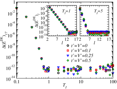
Figure 1: (color online). Relative difference $\Delta(E)_{17}$ between the last 2 orders in the NLCE calculation of $E^{\text{DE}}$ vs $T_{I}$ for different values of $t^{\prime}=V^{\prime}$ in the final Hamiltonian. For $T_{I}\gtrsim 0.7$, $\Delta(E^{\text{DE}})_{17}$ is zero within machine precision. (Insets) $\Delta(E)_{l}$ vs $l$ for two values of $T_{I}$ and the same quenches as in the main panel. The plots show that $E^{\text{DE}}_{l}$ approaches $E^{\text{DE}}_{18}$ exponentially fast with $l$.

We use these NLCEs to study quenches of hard-core bosons in one-dimensional lattices, with nearest (next-nearest) neighbor hopping $t$ ($t^{\prime}$) and repulsive interaction $V$ ($V^{\prime}$) sup . This model is integrable if $t^{\prime}=V^{\prime}=0$ and nonintegrable otherwise Cazalilla et al. (2011). It has been previously considered in quenches in finite lattices Rigol (2009a), and in studies of the integrability to quantum chaos transition Santos and Rigol (2010a). After the quench, we take $V=t=1$ ($t=1$ sets our unit of energy), while $t^{\prime}=V^{\prime}$ are tuned between 0 and 1. Unless otherwise specified, the initial state is taken to be in thermal equilibrium with temperature $T_{I}$ for $t_{I}=0.5$, $V_{I}=1.5$, and $t^{\prime}_{I}=V^{\prime}_{I}=0$. We restrict our analysis to half-filling (the average number of particles is one half the number of lattice sites). Given the particle-hole symmetry of our model, this is enforced by taking $\mu_{I}=0$. The NLCE is implemented using maximally connected clusters, i.e., for any given number of lattice sites $l$, only the cluster with $l$ contiguous sites is used sup .

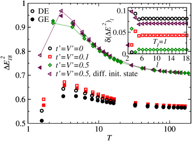
Figure 2: Last order ($l=18$) of the NLCE of $\Delta E^{2}$ in the DE (open symbols) and the GE (filled symbols) vs $T$, for quenches with $T_{I}\geq 1$. The quenches with a different initial state ($t^{\prime}=V^{\prime}=0.5$) have $t_{I}=0.5$, $V_{I}=1.5$, $t^{\prime}_{I}=V^{\prime}_{I}=0.5$, while $t=V=1$ as in the other quenches. Lines joining the data points for the quenches with $t^{\prime}=V^{\prime}=0.5$ are meant to guide the eye and show that $\Delta E^{2}$ in the DE depends on the initial state. The inset shows $\delta(\Delta E^{2})_{l}$ vs $l$ for $T_{I}=1$ for the same quenches as in the main panel.

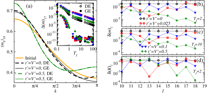
Figure 3: Momentum distribution and kinetic energy $K$ after a quench. (a), Last order ($l=18$) of the NLCE for the momentum distribution in the initial state ($T_{I}=2$), and in the DE and the GE after quenches with $t^{\prime}=V^{\prime}=0$ and 0.5. (b)–(d), Relative differences between $(m_{k})^{\text{DE}}_{l}$ and $(m_{k})^{\text{GE}}_{18}$ [(b),(c)] and between $K^{\text{DE}}_{l}$ and $K^{\text{GE}}_{18}$ (d) vs $l$ in four sets of quenches with $T_{I}=2$ [(b),(d)] and $T_{I}=10$ (c). These results provide strong evidence that thermalization occurs in nonintegrable systems but fails at integrability. Inset in (a), open (filled) symbols report the relative difference between $(m_{k})^{\text{DE}}_{l}$ [$(m_{k})^{\text{GE}}_{l}$] in the last 2 orders of the NLCE vs $T_{I}$, for the same quenches as in (b)–(d). For ease of display, there is a four decade gap in the $y$ axis of the inset.

After a quench, it is important to accurately determine the mean energy per site in the DE ($E^{\text{DE}}$). It defines, along with the mean number of particles per site (fixed here to be 1/2), the thermal ensemble used to determine whether observables thermalize. Since observables within NLCEs are computed using a finite number of clusters, we denote the result obtained when adding the contribution of all clusters with up to $l$ sites as $\mathcal{O}^{\text{ens}}_{l}$ (the superscript “ens” is used for DE or GE). To assess how close $\mathcal{O}^{\text{ens}}_{l}$ is to the thermodynamic limit result, we compute the difference between $\mathcal{O}^{\text{ens}}_{l}$ and the result for the highest order available ($l=18$ in our calculations)

$$\Delta(\mathcal{O}^{\text{ens}})_{l}=\frac{|\mathcal{O}^{\text{ens}}_{l}-\mathcal{O}^{\text{ens}}_{18}|}{|\mathcal{O}^{\text{ens}}_{18}|}.$$ (1)

When $\Delta(\mathcal{O}^{\text{ens}})_{l}$ becomes independent of $l$, and zero within machine precision, we expect that $\mathcal{O}^{\text{ens}}_{l}$ has converged to the thermodynamic limit result.

The accuracy of our calculation for $E^{\text{DE}}$ can be inferred from Fig. 1, where we plot $\Delta(E^{\text{DE}})_{17}$ vs $T_{I}$ for several quenches. For $T_{I}\gtrsim 0.7$, $E^{\text{DE}}_{17}=E^{\text{DE}}_{18}$ within machine precision. The insets in Fig. 1 depict $\Delta(E^{\text{DE}})_{l}$ vs $l$ for $T_{I}=1$ and 2. These plots show that (i) $E^{\text{DE}}_{l}$ approaches $E^{\text{DE}}_{18}$ exponentially fast with $l$, and (ii) with increasing $T_{I}$, fewer orders are required for $E^{\text{DE}}_{l}$ to converge to an $l$-independent result (expected to be $E^{\text{DE}}$ in the thermodynamic limit) within machine precision. The exponential convergence of $E^{\text{DE}}_{l}$ with $l$ shows that NLCEs are fundamentally different from exact diagonalization. In the latter, results usually converge as a power law in system size sup .

Once $E^{\text{DE}}$ is known, one can define an effective temperature after the quench ($T$) as that of a grand-canonical ensemble such that $E^{\text{GE}}=E^{\text{DE}}$. (Here, all effective temperatures are computed, enforcing that the relative energy difference between $E^{\text{DE}}_{18}$ and $E^{\text{GE}}_{18}$ is smaller than $10^{-11}$.) A question that arises is whether one can make simple measurements in a system after a quench that will distinguish it from one in thermal equilibrium. The dispersion of the energy per site $\Delta E^{2}=(\langle\hat{H}^{2}\rangle-\langle\hat{H}\rangle^{2})/L$ are a good candidate (see Ref. sup for another one). In thermal equilibrium they depend on the ensemble used to compute them. $\Delta E^{2}=0$ in the microcanonical ensemble while $\Delta E^{2}\geq 0$ in the canonical ensemble and the GE. $\Delta E^{2}$ is also of interest because, in the latter two ensembles, the specific heat $C_{v}=(1/L)\partial\langle\hat{H}\rangle/\partial T\propto\Delta E^{2}$.

In what follows, in order to quantify how order by order the DE prediction for an observable compares to the GE result in the last order, we define the relative difference

$$\delta(\mathcal{O})_{l}=\frac{|\mathcal{O}^{\text{DE}}_{l}-\mathcal{O}^{\text{GE}}_{18}|}{|\mathcal{O}^{\text{GE}}_{18}|}.$$ (2)

We make sure that, for all results reported for $\delta(\mathcal{O})_{l}$, the analysis of $\Delta(\mathcal{O}^{\text{GE}})_{l}$ suggests that $\mathcal{O}^{\text{GE}}_{18}$ has converged to the thermodynamic limit result.

In the main panel in Fig. 2, we plot $\Delta E^{2}$ in the DE (empty symbols) and in the GE (filled symbols) vs $T$ for quenches with $T_{I}\geq 1$. These results, particularly the ones at the lowest temperatures, make it apparent that $\Delta E^{2}$ is different in the DE and the GE. Moreover, as shown in Fig. 2 for quenches with different initial states but the same final Hamiltonian ($t^{\prime}=V^{\prime}=0.5$), $\Delta E^{2}$ in the DE depends on the initial state. The relative differences $\delta(\Delta E^{2})_{l}$, between $\Delta E^{2}$ in the DE for order $l$ and in the last order in the GE are plotted in the insets in Fig. 2(a) vs $l$. They show that the nonzero differences seen in the main panels between $\Delta E^{2}$ in the DE and the GE are fully converged and are thus expected to be the ones in the thermodynamic limit. The fact that $\Delta E^{2}$ in the DE and the GE agree with each other as $T_{I}\rightarrow\infty$ (main panel in Fig. 2) is universal. This is because as $T_{I}\rightarrow\infty$, the initial thermal ensemble becomes a completely random ensemble. Consequently, the DE after a quench and the corresponding GE also become completely random ensembles and give identical results for all observables independently of the model He and Rigol (2012); Torres-Herrera and Santos (2013).

The question we address next is whether experimentally relevant observables, which are ensemble independent in thermal equilibrium in the thermodynamic limit, thermalize after a quench. Specifically, we consider the momentum distribution $m_{k}$ sup and the kinetic energy associated with nearest neighbor hoppings $K=-t\sum_{i}\langle\hat{b}^{\dagger}_{i}\hat{b}_{i+1}\rangle$. In Fig. 3(a), we show $m_{k}$ in the initial state ($T_{I}=2$), and in the DE and the corresponding GE after quenches with $t^{\prime}=V^{\prime}=0$ (integrable) and $t^{\prime}=V^{\prime}=0.5$ (nonintegrable). The DE and GE results are indistinguishable in the nonintegrable case, indicating thermalization, while they are clearly different at integrability, indicating the lack thereof.

When quantifying the differences between $m_{k}$ in the DE and the GE, we find that while the convergence of $m_{k}^{\text{GE}}$ is qualitatively similar to that of the observables analyzed previously, the same is not true for $m_{k}^{\text{DE}}$. As shown in the inset in Fig. 3(a), for $T_{I}\gtrsim 2$, the results for $m_{k}^{\text{GE}}$ are converged within machine precision for all values of $t^{\prime}=V^{\prime}$ shown, while the ones for $m_{k}^{\text{DE}}$ are not. This indicates that clusters larger than those accessible here contribute to $m_{k}^{\text{DE}}$ in the thermodynamic limit and, as such, a careful scaling analysis is required to conclude whether thermalization occurs or not. We have found this to be true for other few-body observables such as $K$.

In Figs. 3(b) and 3(c), we show the relative difference $\delta(m)_{l}$ [defined in the same spirit as Eq. (2), see Ref. sup ] between $m_{k}$ in the DE for order $l$ and in the last order in the GE vs $l$ for $T_{I}=2$ [Fig. 3(b)] and $T_{I}=10$ [Fig. 3(c)]. The results are qualitatively similar at both temperatures but show different behavior depending on the value of $t^{\prime}=V^{\prime}$. At integrability, $\delta(m)_{l}$ approaches finite values as $l$ increases, so $m_{k}$ is not expected to thermalize in the thermodynamic limit. The convergence uncertainty in $m_{k}^{\text{DE}}$ is not significant in this case because $\delta(m)_{18}$ [Figs. 3(b)] is almost 2 orders of magnitude greater than $\Delta(S)_{17}$ [inset in Fig. 3(a)].

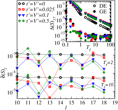
Figure 4: Entropy after a quench. Relative difference $\delta(S)_{l}$ between $S^{\text{DE}}_{l}$ and $S^{\text{GE}}_{18}$ vs $l$ in quenches with $T_{I}=2$ (top four plots) and $T_{I}=10$ (bottom four plots). (Inset) Open (filled) symbols report the relative difference $\Delta(S)_{17}$ between $S^{\text{DE}}_{l}$ ($S^{\text{GE}}_{l}$) in the last 2 orders of the NLCE expansion vs $T_{I}$, for the same quenches as in the main panel. The results in this figure are qualitatively similar to those in Fig. 3. For ease of display, there is a four decade gap in the $y$ axis of the inset.

In the nonintegrable regime with $t^{\prime}=V^{\prime}>0.1$, we find that $\delta(m)_{l}$ in Figs. 3(b) and 3(c) consistently decreases with increasing $l$ and that $\delta(m)_{18}\lesssim\Delta(m)_{17}$ [see the inset in Fig. 3(a)]. These results suggest that nonzero values of $\delta(m)_{l}$ stem from the lack of convergence of $m_{k}^{\text{DE}}$ and will vanish as $l\rightarrow\infty$. Hence, our calculations provide strong evidence that, in the thermodynamic limit, $m^{\text{DE}}_{k}=m^{\text{GE}}_{k}$. When approaching the integrable point ($t^{\prime}=V^{\prime}=0.025$ in the plots), we find that the convergence of $m_{k}^{\text{DE}}$ worsens [see, e.g., $\Delta(m^{\text{DE}})_{17}$ in the inset in Fig. 3(a)] and $\delta(m)_{l}$ vs $l$ exhibits erratic behavior sup . For systems in equilibrium, such behavior is usually seen close to a phase transition, which suggests that in quantum quenches a phase transition to thermalization occurs as soon as one breaks integrability. This can be understood as, on approaching an integrable point, larger systems sizes are needed for the onset of eigenstate thermalization Santos and Rigol (2010a, b); Neuenhahn and Marquardt (2012); Steinigeweg et al. (2013), which results in larger cluster sizes needed for the series to converge to the thermal prediction. We have obtained qualitatively similar results when studying other few-body observables. In Fig. 3(d) we plot results for $\delta(K)_{l}$ vs $l$, which are qualitatively similar to those for $\delta(m)_{l}$ in Figs. 3(b) and 3(c).

Further evidence supporting the robustness of the picture above is provided by the entropy. In the DE, the von Neumann entropy $S^{\text{DE}}=-\sum_{\alpha}W_{\alpha}\ln(W_{\alpha})$ has been argued to satisfy all properties expected of a thermodynamic entropy Polkovnikov (2011) and to agree (disagree) with the thermal entropy in quenches involving nonintegrable (integrable) systems where thermalization occurs (fails to occur) Santos et al. (2011). As shown in Fig. 4, the relative differences $\delta(S)_{l}$ between $S^{\text{DE}}_{l}$ and $S^{\text{GE}}_{18}$ vs $l$ behave qualitatively similarly to $\delta(m)_{l}$ and $\delta(K)_{l}$ in Figs. 3(b)–3(d). The convergence of the NLCE for the entropy (inset in Fig. 4) is also qualitatively similar to that of $m_{k}$ (inset in Fig. 3). Hence, our results provide further support the picture that $S^{\text{DE}}$ agrees (disagrees) with $S^{\text{GE}}$ when few-body observables thermalize (do not thermalize).

In summary, we have introduced NLCEs for the DE and shown that they can be used to study generic quenches in lattice systems in the thermodynamic limit. In the quenches studied here, NLCEs provided strong evidence that nonintegrable systems thermalize while integrable systems do not, and that a phase transition to thermalization may occur as soon as one breaks integrability. We plan to explore next whether NLCEs can be used to study dynamics, which would allow one to address fundamental questions related to prethermalization Kinoshita et al. (2006); Gring et al. (2012); Berges et al. (2004); Moeckel and Kehrein (2008); Kollar et al. (2011) and to the time scales needed to observe thermalization in isolated systems.

Hamiltonian. The hard-core boson Hamiltonian reads

$$\hat{H} = \sum_{i}\left\{-t\left(\hat{b}^{\dagger}_{i}\hat{b}_{i+1}+\textrm{H.c.}\right)+V\left(\hat{n}_{i}-\dfrac{1}{2}\right)\left(\hat{n}_{i+1}-\dfrac{1}{2}\right)\right.$$ (3)

$$- \left.t^{\prime}\left(\hat{b}^{\dagger}_{i}\hat{b}_{i+2}+\textrm{H.c.}\right)+V^{\prime}\left(\hat{n}_{i}-\dfrac{1}{2}\right)\left(\hat{n}_{i+2}-\dfrac{1}{2}\right)\right\},$$

where $\hat{b}^{\dagger}_{i}(\hat{b}_{i})$ denote the hard-core boson creation (annihilation) operators, and $\hat{n}_{i}=\hat{b}^{\dagger}_{i}\hat{b}_{i}$ the number operator. In addition to the bosonic commutation relations $[\hat{b}_{i},\hat{b}^{\dagger}_{j}]=\delta_{ij}$, those operators satisfy the constraints $\hat{b}^{{\dagger}2}_{i}=\hat{b}^{2}_{i}=0$, which prevent multiple occupancies of lattice sites in all physical states.

Momentum distribution $m_{k}$. The momentum distribution function is defined as the Fourier transform $\hat{m}_{k}=(1/L)\sum_{jj^{\prime}}e^{ik(j-j^{\prime})}\hat{\rho}_{jj^{\prime}}$ of the one-particle density matrix $\hat{\rho}_{jj^{\prime}}=\hat{b}_{j}^{\dagger}\hat{b}_{j^{\prime}}$. In our calculations, we compute $m_{k}$ in 100 equidistant $k$ points between $k=0$ and $\pi$. For $m_{k}$, in the same spirit of Eq. (1) in the main text, we define

$$\Delta(m^{\text{ens}})_{l}=\frac{\sum_{k}|(m_{k})^{\text{ens}}_{l}-(m_{k})^{\text{ens}}_{18}|}{\sum_{k}(m_{k})^{\text{ens}}_{18}},$$ (4)

where by “ens” we mean DE or GE, and, in the same spirit of Eq. (2) in the main text, we define

$$\delta(m)_{l}=\frac{\sum_{k}|(m_{k})^{\text{DE}}_{l}-(m_{k})^{\text{GE}}_{18}|}{\sum_{k}(m_{k})^{\text{GE}}_{18}}.$$ (5)

Linked-cluster expansions. In a linked-cluster expansion Oitmaa et al. (2006), the expectation value of an extensive observable $\hat{\mathcal{O}}$ per lattice site $\mathcal{O}=\langle\hat{\mathcal{O}}\rangle/L$ ($L$ is the number of lattice sites), in the thermodynamic limit, is computed as the sum over the contributions from all clusters $c$ that can be embedded on the lattice

$$\mathcal{O}=\sum_{c}M(c)\times W_{\mathcal{O}}(c).$$ (6)

$M(c)$ is the number of ways per site in which cluster $c$, with all sites connected, can be embedded on the lattice. [$M(c)$ is known as the multiplicity of $c$.] $W_{\mathcal{O}}(c)$ is the weight of that cluster for the observable $\mathcal{O}$, which is calculated using the inclusion-exclusion principle:

$$W_{\mathcal{O}}(c)=\mathcal{O}(c)-\sum_{s\subset c}W_{\mathcal{O}}(s),$$ (7)

where the sum runs over all connected sub-clusters of $c$ and

$$\mathcal{O}(c)={\textrm{Tr}[\hat{\mathcal{O}}\,\hat{\rho}_{c}]}/{\textrm{Tr}[\hat{\rho}_{c}]}$$ (8)

is the expectation value of $\hat{\mathcal{O}}$ calculated for the finite cluster $c$, with many-body density matrix $\hat{\rho}_{c}$.

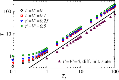
Figure 5: Effective temperature after the quench vs $T_{I}$, for the same quenches as in Fig. 1 in the main text. We also show results for a quench with with a different initial state with $t^{\prime}=V^{\prime}=0$ and $t_{I}=1.5$, $V_{I}=0.5$ ($t^{\prime}_{I}=V^{\prime}_{I}=0$ and $t=V=1$, as in all other quenches), which illustrates that $T$ can be lower than $T_{I}$. The straight line depicts $T=T_{I}$.

NLCE with maximally connected clusters. An important feature of NLCEs, which is not present in other linked-cluster expansions, is that one has quite some freedom in the selection of the building blocks used to carry out the expansion. One can use sites, bonds, and even squares or triangles depending on the geometry of the lattice Rigol et al. (2006, 2007b). (A pedagogical introduction to NLCEs and their implementation can be found in Ref. Tang et al. (2013).) Here, we use the maximally connected clusters. For $l$ sites, the maximally connected cluster is the cluster with $l$ contiguous sites in which all nearest and next-nearest neighbor hoppings and interactions defined by the Hamiltonian are included. It is the only connected cluster with $l$ sites if $t^{\prime}=V^{\prime}=0$. Such an expansion is expected to be best suited when $t^{\prime}=V^{\prime}$ are small compared to $t$ and $V$. In our calculations, we carry out the NLCE computing observables in all maximally connected clusters with up to $l=18$.

Effective temperature $T$ after the quench. In Fig. 5, we show $T$ for the quenches in Fig. 1 in the main text. While $T$ can be seen to be greater than $T_{I}$ in those quenches, this need not always occur. A quench, if $T_{I}>0$, can effectively cool a system. As an example, in Fig. 5 we also show $T$ for quenches in which $t^{\prime}=V^{\prime}=0$ after the quench, while $t_{I}=1.5$, $V_{I}=0.5$, where one can see that $T<T_{I}$ for $T_{I}\gtrsim 1$.

Dispersion of the density.

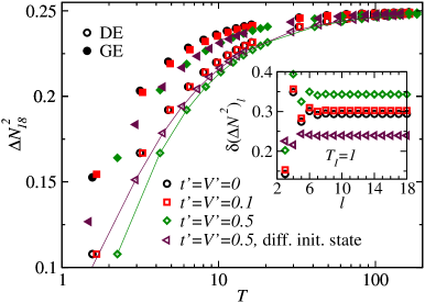
Figure 6: Last order ($l=18$) of the NLCE of $\Delta N^{2}$ in the DE (open symbols) and the GE (filled symbols) vs $T$, for quenches with $T_{I}\geq 1$. The quenches with a different initial state ($t^{\prime}=V^{\prime}=0.5$) have $t_{I}=0.5$, $V_{I}=1.5$, $t^{\prime}_{I}=V^{\prime}_{I}=0.5$, while $t=V=1$ as in the other quenches. Lines joining the data points for the quenches with $t^{\prime}=V^{\prime}=0.5$ are meant to guide the eye and show that $\Delta N^{2}$ in the DE depends on the initial state. The inset shows $\delta(\Delta N^{2})_{l}$ vs $l$ for $T_{I}=1$ for the same quenches as in the main panel.

In addition to the dispersion of the energy discussed in the main text, the dispersion of the total number of particles (per site), $\Delta N^{2}=(\langle\hat{N}^{2}\rangle-\langle\hat{N}\rangle^{2})/L$, also allow one to distinguish the DE from the GE. In thermal equilibrium, they depend on the ensemble used to compute them. $\Delta N^{2}=0$ in the microcanonical and canonical ensembles, while it can be different from zero only in the grand-canonical ensemble. $\Delta N^{2}$ is also of interest because, in the grand-canonical ensemble, the compressibility $\kappa=(1/L)\partial\langle\hat{N}\rangle/\partial\mu=\Delta N^{2}/T$.

In the main panel in Fig. 6, we plot $\Delta N^{2}$ in the DE (empty symbols) and in the GE (filled symbols) vs $T$ for quenches with $T_{I}\geq 1$. These results, particularly the ones at the lowest temperatures, make it apparent that $\Delta N^{2}$ is different in the DE and the GE. Moreover, for quenches with different initial states but the same final Hamiltonian (with $t^{\prime}=V^{\prime}=0.5$), $\Delta N^{2}$ in the DE can be seen to depend on the initial state. The relative differences $\delta(\Delta N^{2})_{l}$ between $\Delta N^{2}$ in the DE for order $l$ and in the last order in the GE are plotted vs $l$ in the inset in Fig. 6. They show that the nonzero differences seen in the main panel between $\Delta N^{2}$ in the DE and the GE are fully converged and are thus expected to be the ones in the thermodynamic limit.

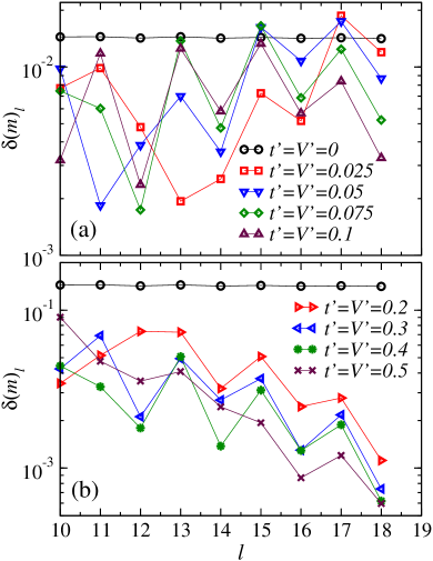
Figure 7: Relative differences between $(m_{k})^{\text{DE}}_{l}$ and $(m_{k})^{\text{GE}}_{18}$ vs $l$ in nine sets of quenches with $T_{I}=2$.

Convergence of the DE results close to the integrable point. In the main text we discussed that as one approaches the integrable point $\delta(m)_{l}$ vs $l$ exhibits erratic behavior, and that this is the result of the worsening of the convergence of $m_{k}^{\text{DE}}$. In systems in equilibrium such a behavior is usually seen close to phase transitions, so we argued that a phase transition to thermalization may occur as soon as one breaks integrability.

In order to supplement the results in Fig. 3 in the main text, so that such an erratic behavior on approaching integrability is better seen by comparing to results as one departs from integrability, in Fig. 7 we plot $\delta(m)_{l}$ vs $l$ for almost three times as many values of $t^{\prime}=V^{\prime}\neq 0$ as those in the main text. In Fig. 7(a) one can see that, for $t^{\prime}=V^{\prime}=0.025$ and $t^{\prime}=V^{\prime}=0.05$, $\delta(m)_{l}$ first decreases and then increases as $l$ increases. For $t^{\prime}=V^{\prime}=0.075$, again $\delta(m)_{l}$ first decreases, then increases, and for the largest values of $l$ it appears to decrease again. The latter behavior becomes more evident for $t^{\prime}=V^{\prime}=0.1$. All results for nonzero $t^{\prime}=V^{\prime}\lesssim 1$ are also characterized by very large oscillations in the values of $\delta(m)_{l}$, which are not present at integrability. On the other hand, the results for $t^{\prime}=V^{\prime}>1$ in Fig. 7(b) offer a different picture. $\delta(m)_{l}$ consistently decreases with increasing $l$, which supports the view that thermalization occurs.

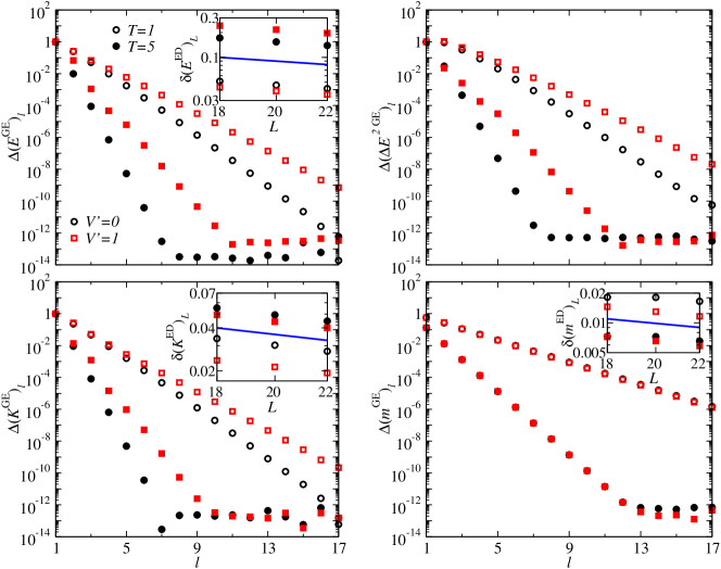
Figure 8: Open (filled) symbols report the relative differences $\Delta(E^{\text{GE}})_{l}$ (a), $\Delta(\Delta E^{2\,\text{GE}})_{l}$ (b), $\Delta(K^{\text{GE}})_{l}$ (c), and $\Delta(m^{\text{GE}})_{17}$ (d) vs $l$ for $T=1$ ($T=5$). Results are presented for $V^{\prime}=0$ (circles) and $V^{\prime}=1.0$ (squares). In all cases one can see an exponential decrease of the differences with increasing cluster size. In the insets in (a), (c), and (d) we show log-log plots of relative differences between results of full exact diagonalization in systems with periodic boundary conditions ($L=18,\,20$ and 22 sites) and NLCE results with $l=18$. In this case one can see that, as expected, the results are consistent with power law scaling in $L$. We have included straight lines in the insets explicitly depicting $1/L$ scaling.

Convergence of NLCEs vs exact diagonalization. In Fig. 8, we show relative differences between NLCE results for four observables when all contributions from clusters with up to $l$ sites are added and the results for $l=18$ (the highest order in the NLCE calculation that we have computed) vs $l$. Those relative differences were defined in Eq. (1) in the main text and in Eq. (5) here. We took as Hamiltonian Eq. (3) when $t^{\prime}=0$, which was systematically studied using exact diagonalization in Ref. Santos and Rigol (2010b). One can see in all panels in Fig. 8 that the relative differences decrease exponentially fast with the order $l$ of the NLCE calculation (note that results are presented for two temperatures $T=1$ and $T=5$).

In the insets in Figs. 8(a), 8(c), and 8(d), we report relative differences between results obtained using full exact diagonalization (ED) in systems with periodic boundary conditions ($L=18,\,20$, and 22 sites) Santos and Rigol (2010b) and the NLCE results for $l=18$

$$\delta(\mathcal{O}^{\text{ED}})_{L}=\frac{|\mathcal{O}^{\text{ED}}_{L}-\mathcal{O}^{\text{GE}}_{18}|}{|\mathcal{O}^{\text{GE}}_{18}|}.$$ (9)

and

$$\delta(m^{\text{ED}})_{L}=\frac{\sum_{k}|(m_{k})^{\text{ED}}_{L}-(m_{k})^{\text{GE}}_{18}|}{\sum_{k}(m_{k})^{\text{GE}}_{18}},$$ (10)

where the sum in Eq. (10) is restricted to the values of $k$ that are available in the specific cluster with periodic boundary conditions used in the exact diagonalization calculation. These differences exhibit a scaling that is consistent with $1/L$, as expected. They make evident that the scaling (and ultimately the accuracy) of the results obtained using NLCEs and ED are fundamentally different, namely, exponential (NLCEs) vs power law (ED).

References

- Rigol et al. (2008) M. Rigol, V. Dunjko, and M. Olshanii, Nature 452, 854 (2008).
- Cazalilla and Rigol (2010) M. A. Cazalilla and M. Rigol, New J. Phys. 12, 055006 (2010).
- Dziarmaga (2010) J. Dziarmaga, Adv. Phys. 59, 1063 (2010).
- Polkovnikov et al. (2011) A. Polkovnikov, K. Sengupta, A. Silva, and M. Vengalattore, Rev. Mod. Phys. 83, 863 (2011).
- Kinoshita et al. (2006) T. Kinoshita, T. Wenger, and D. S. Weiss, Nature 440, 900 (2006).
- Gring et al. (2012) M. Gring, M. Kuhnert, T. Langen, T. Kitagawa, B. Rauer, M. Schreitl, I. Mazets, D. A. Smith, E. Demler, and J. Schmiedmayer, Science 337, 1318 (2012).
- Rigol et al. (2007a) M. Rigol, V. Dunjko, V. Yurovsky, and M. Olshanii, Phys. Rev. Lett. 98, 050405 (2007a).
- Rigol (2009a) M. Rigol, Phys. Rev. Lett. 103, 100403 (2009a).
- Rigol (2009b) M. Rigol, Phys. Rev. A 80, 053607 (2009b).
- Trotzky et al. (2012) S. Trotzky, Y.-A. Chen, A. Flesch, I. P. McCulloch, U. Schollwöck, J. Eisert, and I. Bloch, Nature Phys. 8, 325 (2012).
- Reimann (2008) P. Reimann, Phys. Rev. Lett. 101, 190403 (2008).
- Linden et al. (2009) N. Linden, S. Popescu, A. J. Short, and A. Winter, Phys. Rev. E 79, 061103 (2009).
- Deutsch (1991) J. M. Deutsch, Phys. Rev. A 43, 2046 (1991).
- Srednicki (1994) M. Srednicki, Phys. Rev. E 50, 888 (1994).
- Kollath et al. (2007) C. Kollath, A. M. Läuchli, and E. Altman, Phys. Rev. Lett. 98, 180601 (2007).
- Manmana et al. (2007) S. R. Manmana, S. Wessel, R. M. Noack, and A. Muramatsu, Phys. Rev. Lett. 98, 210405 (2007).
- Eckstein et al. (2009) M. Eckstein, M. Kollar, and P. Werner, Phys. Rev. Lett. 103, 056403 (2009).
- Bañuls et al. (2011) M. C. Bañuls, J. I. Cirac, and M. B. Hastings, Phys. Rev. Lett. 106, 050405 (2011).
- Essler et al. (2014) F. H. L. Essler, S. Kehrein, S. R. Manmana, and N. J. Robinson, Phys. Rev. B 89, 165104 (2014).
- Oitmaa et al. (2006) J. Oitmaa, C. Hamer, and W.-H. Zheng, Series Expansion Methods for Strongly Interacting Lattice Models (Cambridge University Press, Cambridge, 2006).
- (21) See the Suplementary Materials.
- Rigol et al. (2006) M. Rigol, T. Bryant, and R. R. P. Singh, Phys. Rev. Lett. 97, 187202 (2006).
- Rigol et al. (2007b) M. Rigol, T. Bryant, and R. R. P. Singh, Phys. Rev. E 75, 061118 (2007b).
- Tang et al. (2013) B. Tang, E. Khatami, and M. Rigol, Comput. Phys. Commun. 184, 557 (2013).
- Rigol et al. (2007c) M. Rigol, T. Bryant, and R. R. P. Singh, Phys. Rev. E 75, 061119 (2007c).
- Tang et al. (2012) B. Tang, T. Paiva, E. Khatami, and M. Rigol, Phys. Rev. Lett. 109, 205301 (2012).
- Cazalilla et al. (2011) M. A. Cazalilla, R. Citro, T. Giamarchi, E. Orignac, and M. Rigol, Rev. Mod. Phys. 83, 1405 (2011).
- Santos and Rigol (2010a) L. F. Santos and M. Rigol, Phys. Rev. E 81, 036206 (2010a).
- He and Rigol (2012) K. He and M. Rigol, Phys. Rev. A 85, 063609 (2012).
- Torres-Herrera and Santos (2013) E. J. Torres-Herrera and L. F. Santos, Phys. Rev. E 88, 042121 (2013).
- Santos and Rigol (2010b) L. F. Santos and M. Rigol, Phys. Rev. E 82, 031130 (2010b).
- Neuenhahn and Marquardt (2012) C. Neuenhahn and F. Marquardt, Phys. Rev. E 85, 060101 (2012).
- Steinigeweg et al. (2013) R. Steinigeweg, J. Herbrych, and P. Prelovšek, Phys. Rev. E 87, 012118 (2013).
- Polkovnikov (2011) A. Polkovnikov, Ann. Phys. 326, 486 (2011).
- Santos et al. (2011) L. F. Santos, A. Polkovnikov, and M. Rigol, Phys. Rev. Lett. 107, 040601 (2011).
- Berges et al. (2004) J. Berges, S. Borsányi, and C. Wetterich, Phys. Rev. Lett. 93, 142002 (2004).
- Moeckel and Kehrein (2008) M. Moeckel and S. Kehrein, Phys. Rev. Lett. 100, 175702 (2008).
- Kollar et al. (2011) M. Kollar, F. A. Wolf, and M. Eckstein, Phys. Rev. B 84, 054304 (2011).