Executive Summary

The photometer section of SPIRE is one of the key instruments on board of Herschel. Its legacy depends very much on how well the scanmap observations that it carried out during the Herschel mission can be converted to high quality maps. In order to have a comprehensive assessment on the current status of SPIRE map-making, as well as to provide guidance for future development of the SPIRE scan-map data reduction pipeline, we carried out a test campaign on SPIRE map-making. In this report, we present results of the tests in this campaign. The goals are: (1) Compare the map-makers in the SPIRE pipeline with other mapmakers. (2) In particular, identify the strengths and limitations of different mapmakers in dealing with the known SPIRE map-making issues, such as the cooler burp effect. (3) Assess the resolution-enhancement capabilities of the super-resolution mappers, as compared to the destriper (the pipeline default), and investigate their applicability to various kinds of data as well as caveats or pitfalls to avoid. (4) Enable users to choose the right map-maker for their science. (5) Provide guidance for future development of the SPIRE scan-map data reduction pipeline.

For these purposes, 13 test cases were generated, including data sets obtained in different observational modes and scan speeds, with different map sizes, source brightness, and levels of complexity of the extended emission. They also include observations suffering from the “cooler burp” effect, and those having strong large-scale gradients in the background radiation. The input data for these test cases are time-ordered data (TODs). The map-making process turns the TODs into maps. Among the test cases, 8 are simulated and 5 are real observations.

Comparing to real observations, a simulated test case has the advantage of possessing the “truth”, namely the sky model, based on which the simulation is carried out. The truth map provides an unbiased standard against which test maps made by different map-makers are to be compared. Allowing for the effects of noise in a given map, deviations from the truth can be used as objective measures for the bias introduced by the map-making process. In the simulations, TODs were generated using two layers of data: a noise layer taken from real SPIRE observations of dark fields (this allows the simulation to include both instrumental noise and confusion noise), and a truth layer which is a sky-model map based either on a real Spitzer 24$\mu m$ map or a map of artificial sources.

Seven map-makers participated in this test campaign, including (1) Naive mapper (default of the SPIRE standard pipeline until HIPE 8); (2) Destriper in two flavors: (i) Destriper-P0: Destriper with polynomial-order = 0 (default of SPIRE standard pipeline since HIPE 9), and (ii) Destriper-P1: Destriper with polynomial-order = 1 ; (3) Scanamorphos; (4) SANEPIC (GLS mapmaker); (5) Unimap (GLS mapmaker); (6) HiRes (super-resolution map-maker); (7) SUPREME (super-resolution map-maker). Because of time constraints, not all map-makers processed all the test cases (see Table 2 for details). Table 1: Test Cases Processed by Different Map-Makers Case Name Map-Maker N D Sc SA U H SU 1 Nominal Sources $\surd$ $\surd$ $\surd$ $\surd$ $\surd$ $\surd$ $\surd$ 2 Nominal Cirrus $\surd$ $\surd$ $\surd$ $\surd$ 3 Nominal Dark $\surd$ $\surd$ $\surd$ $\surd$ 4 Nominal M51 $\surd$ $\surd$ $\surd$ $\surd$ 5 Fast-scan Sources $\surd$ $\surd$ $\surd$ $\surd$ $\surd$ 6 Fast-scan MK Center $\surd$ $\surd$ $\surd$ $\surd$ $\surd$ 7 Fast-scan Dark $\surd$ $\surd$ $\surd$ $\surd$ 8 Parallel Sources $\surd$ $\surd$ $\surd$ $\surd$ 9 Parallel Mk Center $\surd$ $\surd$ $\surd$ $\surd$ 10 Parallel Cirrus $\surd$ $\surd$ $\surd$ $\surd$ $\surd$ $\surd$ $\surd$ 11 Parallel Dark $\surd$ $\surd$ $\surd$ $\surd$ 12 Nominal NGC 628 $\surd$ $\surd$ $\surd$ $\surd$ $\surd$ $\surd$ 13 Para-fast Hi-Gal-L30 $\surd$ $\surd$ $\surd$ $\surd$ $\surd$ $\surd$

Results of tests are presented in the framework of four sets of metrics:

(1) Deviation from the truth. These metrics include: (i) visual examinations of the difference map $\rm Map-Map_{true}$; (ii) a scatter plot of (S – S_true) vs S_true for individual pixels; (iii) slopes of these plots; (iv) absolute deviations: mean and standard deviation of S – S_true; (v) relative deviations: mean and standard deviation of (S – S_true)/S_true. They are applied to maps of 5 simulated test cases (Cases 2, 4, 6, 9, 10) that are based on real MIPS 24$\mu m$ maps (simulated cases based on artificial sources are excluded). The results clearly demonstrate the applicability and limitation of individual map-makers. Destriper-P0 produces the least deviations in most cases, but its maps show artificial stripes for the cases with “cooler burp effect”. Scanamorphos, running with the “galactic option” and without the “relative gain corrections”, can minimize the “cooler burp effect”. However, bright pixels in Scanamorphos maps display large deviations, likely due to a slight positional offset introduced by the mapper, and a slight change in the beam size. Destriper-P1, SANEPIC, and Unimap introduce different types of large spatial scale noise. For SANEPIC, this is likely due to mismatches between the assumptions made in the map-maker and the properties of the test data. For example, SANEPIC assumes that data are circulant, which is not true for the Case 9. For Unimap, the large scale distortion in maps of Case 6 is triggered by the “cooler burp effect”, which the map-maker does not know how to handle. For Naive-mapper (with simple median background removal), many maps show large deviations due to the over-subtraction of the background when extended emission is present.

(2) Spatial (2-D) power spectra. These metrics include (i) plots and comparisons of power spectra of maps made by different map-makers; (ii) for simulated cases, plots and comparisons of the divergence from the truth power spectrum of the maps by different map-makers. Most of the power spectra, either coming from real or simulated data, noise-only or with extended emission, show very similar results. In the “middle part” ($k=[0.1,1]$ arcmin^-1), results among different map-makers vary little: $\sim 1\%$ for cases where a truth map was available as benchmark. At smaller scales ($k>1$ arcmin^-1), the standard Naive mapper produces higher powers than other map-makers, presumably due to the fine-stripes (baseline removal errors) found in its maps. Meanwhile, at the same scale, results of Destriper-P0, Destriper-P1, Unimap, and SANEPIC are always very close, and those of Scanamorphos are usually lower. The low power at high spatial frequencies in Scanamorphos maps is likely due to the fact that, unlike other map-makers, Scanamorphos distributes the signal measured at a sky position among multiple adjacent map pixels. This is equivalent to a map smoothing, which takes away high frequency powers. At larger scales ($k<0.1$ arcmin^-1), again the Naive mapper produces higher powers because of the poor baseline removal, while the results of other map-makers are all comparable. In the special cases with the “cooler burp”, the power spectra of Naive and Destriper-P0 maps are clearly affected, showing much higher power at $k<0.1$ and a peak at $k\sim 1.5$ in the PLW map. No significant effects due to the “cooler burp” are found in results of the other map-makers.

(3) Point source and extended source photometry. These metrics include (i) astrometry of point sources; (ii) point source and extended source photometry; (iii) detection rates of faint point sources, obtained using Starfinder (a point source extractor); (iv) PSF profiles. They are applied to the simulated test cases with artificial sources (Cases 1, 5 and 8). The results show that bright sources in maps made by Scanamorphos have systematically larger position errors ($\,\lower 2.0pt\hbox{${>\atop\hbox{\raise 4.0pt\hbox{$\sim$}}}$}\,0.1$ pixel) than those in maps made by other map-makers, consistent with the results on position offsets in Scanamorphos maps found in Metrics (1) for the deviation from the truth. Photometry for bright point sources in all maps has small errors, indicating good energy conservation by all map-makers. On the other hand, photometry of extended sources in the Naive mapper are significantly affected by a known bias due to the over-subtraction of baselines, while other maps have no such issue. For faint point sources ($\rm f=30\;mJy$), no significant difference is found among results for different map-makers on both detection rate and photometry. Also, there is no significant difference between beam profiles of sources in maps made by different map-makers.

(4) Metrics for super-resolution maps. These metrics are applied to maps made by HiRes and SUPREME, the two super-resolution mappers, and compare them to maps made by the destriper (the pipeline default). They include: (i) visual examinations of the maps; (ii) spatial power spectra; (iii) point source profiles. The results show that SUPREME and HiRes yield similar resolution enhancements (factors of 2-3) at spatial scales around 2 arcmin^-1 for the limited datasets tested at 250 microns. At higher spatial frequencies corresponding to spatial scales smaller than the beam size, there is less power in the SUPREME maps (intentionally, to smooth and reduce the noise at scales smaller than the beam). HiRes contains more power than either SUPREME or Destriper-P0 maps between spatial scales of 15-20 arcseconds. The differences in SUPREME and HiRes arise mainly because SUPREME is tuned to enhance extended emission features, and HiRes is essentially performing a deconvolution in image space.

Summary of Results:

• The Destriper with polynomial order of 0 (Destriper-P0), which is the default map-maker in the SPIRE scanmap pipeline since HIPE 9, performed remarkably well and compared favorably among all map-makers in all test cases except for those suffering from the “cooler burp” effect, as it does not have a mechanism to deal with this effect. In particular, it can handle observations with complex extended emission structures and with large scale background gradient very well.

• In contrast, the Destriper with the polynomial order of 1 (Destriper-P1) compared poorly among its peers, introducing significant artificial large scale gradient in many cases.

• Scanamorphos showed noticeable differences in all comparisons. On the positive side, its maps have the smallest deviation from the truth for faint pixels ($\rm f<0.2Jy$) in nearly all cases. Particularly, as shown in both the difference maps and in the power-spectra, it can handle the “cooler burp” effect very well. On the negative side, for bright pixels ($\rm f>0.2Jy$), its maps show significant deviations from the truth, likely due to a slight positional offset introduced by the mapper as well as a slight change in the beam size. This effect is also seen in the astrometric errors of the bright sources. However the offset is very small ($\sim 0.1pexel$), therefore it does not affect the photometry of both point sources and extended sources, and does not show up in the comparison between beam profiles (resolution: 0.2 pixels). The power spectrum analysis indicates some smoothing of the data compared to the other mapmakers.

• The GLS mapper SANEPIC can also minimize the “cooler burp” effect. It performed quite well in most cases. However, for those cases with strong variations in very large scales (i.e. comparable to the map size), its maps show significant deviations from the truth. This is because some of its assumptions (e.g. TODs are circulant) are invalid for the data.

• Unimap, another participating GLS mapper, is among the best performers in most cases. However, because it does not include a mechanism for handling the “cooler burp”, its maps show significant deviations from the truth in the cases affected by the artifact.

• The Naive-mapper (with simple median background removal) is inferior among its peers in general. The most severe bias it introduces is the over-subtraction of the background when extended emission is present. In the cases where the extended emission is in complex structures, this bias cannot be avoided by simple masks in the background removal.

• The two super-resolution mapmakers, SUPREME and HiRes, yield similar resolution enhancements (factors of 2-3) at spatial scales around 2 arcmin^-1 for the limited datasets tested at 250 microns. At higher spatial frequencies corresponding to spatial scales smaller than the beam size, there is less power in the SUPREME maps (intentionally, to smooth and reduce the noise at scales smaller than the beam). HiRes contains more power than either SUPREME or Destriper-P0 maps between spatial scales of 15-20 arcseconds. The differences in SUPREME and HiRes arise mainly because SUPREME is tuned to enhance extended emission features, and HiRes is essentially performing a deconvolution in image space.

Chapter 1 Introduction and Goals

The current version of the standard SPIRE photometer scanmap data reduction pipeline (in HIPE 11) is doing a reasonably satisfactory job for most observations obtained using the SPIRE Photometer AOTs. Except for some very challenging science goals (e.g. the CIB/CMB anisotropy studies), maps in the Level 2 (or Level 2.5 for parallel mode observations) products of the Standard Product Generation (SPG) pipeline (i.e. the ones coming directly out of the HSA) are already of science quality. In particular, after replacing the median baseline remover by the destriper as the default baseline remover in the HIPE 9 pipeline, there is not much left for an observer to do in order to further improve the quality of a normal SPIRE photometer map, unless some special problems occur for which the solutions have not yet been developed. An example of these remaining problems is the so-called ”cooler burp” effect (affecting a few percent of SPIRE scanmap data): After every SPIRE cooler-recycle, the first 6 hours or so see a steep increase of the temperature of the 300 mK sorption cooler. This causes abnormal drifts in detector timelines, which cannot be corrected by the standard temperature drift correction module in the pipeline, and results in stripes in maps observed during the “cooler burp” period. Another issue with standard SPIRE maps is related to the relatively coarse angular resolutions (beam size $\,\lower 2.0pt\hbox{${>\atop\hbox{\raise 4.0pt\hbox{$\sim$}}}$}\,18^{\prime\prime}$) due to diffraction. Super-resolution mappers that can beat the the diffraction limit and at same time cause minimal artifacts are certainly desirable.

Given the general status of the SPIRE scanmap pipeline, and the remaining issues in the SPIRE map-making, we set the following goals for this SPIRE map-making test campaign:

• Compare the map-makers in the SPIRE pipeline with other mapmakers objectively and comprehensively.

• In particular, identify the strengths and limitations of different mapmakers in dealing with the known SPIRE map-making issues, such as the cooler burp effect.

• Assess the resolution-enhancement capabilities of the super-resolution mappers as compared to the destriper (the pipeline default), and investigate their applicability to various kinds of data, as well as caveats or pitfalls to avoid.

• Enable users to choose the right map-maker for their science.

• Provide guidance for future development of the SPIRE scan-map data reduction pipeline.

In the next chapter, Chapter 2, the test cases examined in this test campaign are presented. Chapter 3 describes the method of the simulations based on which some test cases were generated. Chapter 4 introduces the map-makers participated in the SPIRE map-making test. The test results are presented, in a framework of pre-designed metrics, in Chapter 5. The last chapter is dedicated to a general summary.

Chapter 2 Test Cases

In order to have comprehensive assessments for map-makers, we requested that test cases shall cover the following parameter space of SPIRE scanmap observations: (1) observation mode (nominal/parallel, scan speed, sampling rate); (2) source brightness; (3) map size; (4) depth; (5) complexity of the extended emission. They shall also include examples of: (i) observations suffering from the ”cooler burp” effects; (ii) sky regions with strong large-scale gradient.

Table 2.1: Test Cases

Case	Method	Name	Mode	Scan	Samp	Size	Bands
				speed	rate
				(′′/sec)	(Hz)	($\circ\times\circ$)
1	simulation	Nominal Sources	Nominal	30	16	0.7$\times$0.7	S, M, L
2	simulation	Nominal Cirrus	Nominal	30	16	0.7$\times$0.7	S, L
3	real obs	Nominal Dark	Nominal	30	16	0.7$\times$0.7	S, M, L
4	simulation	Nominal M51	Nominal	30	16	0.7$\times$0.7	S, M, L
5	simulation	Fast-scan Sources	Fast Scan	60	16	3.5$\times$3.5	S, L
6	simulation	Fast-scan MK-Center	Fast Scan	60	16	3.5$\times$3.5	S, L
7	real obs	Fast-scan Dark	Fast Scan	60	16	3.5$\times$3.5	S, L
8	simulation	Parallel Sources	Parallel	20	10	1.3$\times$1.3	S, L
9	simulation	Parallel MK-Center	Parallel	20	10	1.3$\times$1.3	S, L
10	simulation	Parallel Cirrus	Parallel	20	10	1.3$\times$1.3	S, L
11	real obs	Parallel Dark	Parallel	20	10	1.3$\times$1.3	S, L
12	real obs	Nominal NGC 628	Nominal	30	16	0.4$\times$0.4	S, L
13	real obs	Para-fast Hi-Gal-L30	Parallel	60	10	1.9$\times$1.9	S, L

In total 13 test cases were generated. The input data for these test cases are time-ordered data, or TODs. The map-making process turns the TODs into maps. These TODs have the format of the SPIRE Level-1 Photometer Scan Product (PSP). As shown in Table 2.1, the test cases include both real observations (5 cases) and simulated observations (8 cases) in 4 observational modes. In the nominal mode (scan speed = 30$”$/sec, sampling rate = 16 Hz), we have 5 test cases (2 real, 3 simulated). In the fast-scan mode (scan speed = 60$”$/sec, sampling rate = 16 Hz), there are 3 test cases (1 real, 2 simulated). In the parallel mode (sampling rate = 10 Hz), we have 4 test cases (1 real, 3 simulated) in slow scan (scan speed = 20$”$/sec) and 1 real case in fast-scan (scan speed = 60$”$/sec). In order to save time but not to lose information, 3 test cases (Cases 1, 2, and 4) include all 3 SPIRE bands while others include only the PSW and PLW bands.

Chapter 3 Simulations

Comparing to real observations, a simulated test case has the advantage of possessing the “truth”, namely the sky model, based on which the simulation is carried out. The truth map provides an unbiased standard against which test maps made by different map-makers are to be compared. Allowing for the effects of noise in a given map, deviations from the truth can be used as objective measures for the bias introduced by the map-making process.

In the simulations, TODs were generated using two layers of data: (1) noise layer — real SPIRE observations (public data) of a dark field; this allows the simulation to include both instrumental noise and confusion noise; (2) truth layer — a sky-model map based either on a real MIPS 24$\mu m$ map (beam-size $\sim 6^{\prime\prime}$) or a map of artificial sources. Sky-model maps in the “truth layer” are fine sampled (pixel size of $1.25^{\prime\prime}$ – $1.5^{\prime\prime}$), convolved with SPIRE beams (sampled with $1^{\prime\prime}$ pixels), and scaled to desired brightness. For those taken from the real MIPS 24$\mu m$ maps, the scaling factors were set to make the original noise in the MIPS observations negligible compared to that in the noise layer.

The simulation procedure is as follows:

1) take Level-1 data of a real SPIRE observation of a dark field (i.e. the noise layer);

2) take a sky-model map (i.e. the truth layer) and replace its WCS by that of the noise layer;

3) obtain the RA and Dec for every sampling point in the Level-1 timelines of the noise layer;

4) then, read the signal in the sky-model map at the RA and Dec of a given sampling point in the noise layer, and add this signal to the signal of that sampling point in the corresponding Level-1 timeline of the noise layer;

5) do step 4) for all sampling points in the noise layer.

These simulations include instrumental noise, confusion noise, and noise due to glitches. However, they do not include effects due to saturation, pointing error, photon noise contributed by very bright sources. Also, the Level-1 timelines provided by the simulations are already de-glitched using the standard SPIRE pipeline, which may not be desirable for some map-makers (e.g. Unimap). In total, we generated 8 simulated test cases (Table 3.1).

Table 3.1: Simulated Test Cases

Case	Mode	Truth Layer	Noise Layer	Depth
1	Nominal	artificial sources	Lockman-North	7 repeats
2	Nominal	cirrus region	Lockman-North	7 repeats
4	Nominal	M51	Lockman-North	7 repeats
5	Fast-Scan	artificial sources	Lockman-SWIRE	2 repeats
6	Fast-Scan	Galactic center	Lockman-SWIRE	2 repeats
8	Parallel	artificial sources	ELAIS N1	5 repeats
9	Parallel	Galactic center	ELAIS N1	5 repeats
10	Parallel	cirrus region	ELAIS N1	5 repeats

Chapter 4 Map-makers

Seven map-makers participated in the SPIRE map-making test, including (1) Naive mapper (default of SPIRE SPG until HIPE 8); (2) Destriper in two flavors: (i) Destriper-P0: Destriper with polynomial-order = 0 (default of SPIRE SPG since HIPE 9) and (ii) Destriper-P1: Destriper with polynomial-order = 1; (3) Scanamorphos; (4) SANEPIC; (5) Unimap; (6) HiRes; (7) SUPREME. Detailed explanations of these map-makers, written by their authors, are presented in the sections in this chapter.

Because of time constraints, not all map-makers processed all the test cases (though some did). In Table 1, the information on which map-maker processed which test cases is provided with check marks. It should also be noted that, for each test case, two sets of input data (TODs, see Chapter 2) were generated. They were both corrected for the following instrumental effects using the standard SPIRE scanmap data reduction pipeline: (1) glitches; (2) electrical low-pass filter; (3) non-linearity; (4) bolometer time response. Additionally, for Data Set 1, the TOD were also corrected for the detector array temperature drift using the standard pipeline, and the “turn-around” data between individual scans were excluded (so there are gaps between scans). These data were used by the Naive, Destriper, HiRes and SUPREME. For Data Set 2, the TOD were not corrected for the detector array temperature drift; the “turn-around” data were included so there are no gaps between scans. These data were used by Scanamorphos, SANEPIC, and Unimap.

We requested that all map-makers project their maps in the same way. In particular, the crota2 parameter should be 0 (north-up); the pixel sizes should be those of the SPIRE standard (pixel = $6^{\prime\prime}$, $10^{\prime\prime}$, and $14^{\prime\prime}$ for PSW, PMW and PLW maps); and the projection should be tangential in both the RA and Dec directions (RA – TAN, DEC – TAN). These requirements also apply to the “truth” maps in simulated cases (c.f. Chapter 3), to which the test maps are to be compared. It should be noted that the original truth maps are in finer grids (pixel size of $1.25^{\prime\prime}$ – $1.5^{\prime\prime}$). Therefore, in order to facilitate the comparisons, we choose to re-generate the truth maps from simulated noise-free TODs using the SPIRE Naive mapper.

Table 4.1: Test Cases Processed by Different Map-Makers

Case	Name	Map-Maker
		N	D	Sc	SA	U	H	SU
1	Nominal Sources	$\surd$	$\surd$	$\surd$	$\surd$	$\surd$	$\surd$	$\surd$
2	Nominal Cirrus	$\surd$	$\surd$	$\surd$	$\surd$
3	Nominal Dark	$\surd$	$\surd$	$\surd$	$\surd$
4	Nominal M51	$\surd$	$\surd$	$\surd$	$\surd$
5	Fast-scan Sources	$\surd$	$\surd$	$\surd$	$\surd$	$\surd$
6	Fast-scan MK Center	$\surd$	$\surd$	$\surd$	$\surd$	$\surd$
7	Fast-scan Dark	$\surd$	$\surd$	$\surd$	$\surd$
8	Parallel Sources	$\surd$	$\surd$	$\surd$	$\surd$
9	Parallel Mk Center	$\surd$	$\surd$	$\surd$	$\surd$
10	Parallel Cirrus	$\surd$	$\surd$	$\surd$	$\surd$	$\surd$	$\surd$	$\surd$
11	Parallel Dark	$\surd$	$\surd$	$\surd$	$\surd$
12	Nominal NGC 628	$\surd$	$\surd$	$\surd$		$\surd$	$\surd$	$\surd$
13	Para-fast Hi-Gal-L30	$\surd$	$\surd$	$\surd$		$\surd$	$\surd$	$\surd$

4.1 Naïve Mapper (Bernhard Schulz)

4.1.1 Introduction

The Naïve Mapper, for the purposes of this investigation, is considered in combination with the Median offset subtractor, since the SPIRE detector signals include arbitrary and variable offsets that can not be easily cast into calibration tables. The median subtractor component first removes the signal offsets by determining the medians of all unmasked readouts of all detectors in a given Level 1 building block and subtracting these values from their respective timelines. This works on the assumption that a map is dominated by flat sky-background, which is not true in general. Then the Naïve Mapper proper establishes a regular grid of sky bins (map pixels) that covers all coordinates associated with the timelines, and the fluxes of individual readouts are distributed into these sky bins by their celestial positions. The contents of each sky bin are averaged, resulting in a regular rectangular numerical array, called the flux map. An error map and a coverage map of the same dimensions are generated as well, based on the distributions of the readouts within each sky bin and their total number therein. The following will give more algorithmic details and will outline the specific processing of each dataset.

4.1.2 The Software

The input data typically suffers from residual instrumental effects like residual glitches, a residual temperature drift component, and arbitrary constant offsets. In order of severity, the last effect has the strongest impact. The detector offsets change relative to each other depending on detector temperature and telescope background typically at the order of 5 Jy/beam. A simple method to remove these arbitrary offsets is based on the assumption that most of what a detector sees is sky background. The solution is then approximated by subtracting the median from each detector, effectively setting the celestial background level to zero. This works well as long as the primary assumption holds true, but breaks down in crowded fields, typically close to the Galactic Plane or in regions with strong Galactic Cirrus. This method has been used in SPIRE Standard Product Generation (SPG) until HIPE 8 together with the Naïve Mapper and is implemented as Task baselineRemovalMedian() in HIPE.

If also temperature induced residual drifts are present, fit and subtraction of a polynomial can sometimes help. However, large scale source emission at low spatial frequencies will become unreliable as fractions of it will be removed by the method. It is implemented in HIPE as Task baselineRemovalPolynomial().

The Naïve Mapper itself is applied after baseline subtraction. It first establishes a regular grid of sky bins (map pixels) based on the resolution parameter that covers the scanned sky field. For the SPIRE detector arrays 6^′′, 10^′′, and 14^′′ have been established as standard sky bin sizes for the detector arrays PSW, PMW, and PLW respectively, to provide near Nyquist sampled resolution. The Naïve Mapper excludes all ”bad” readouts where flags fit a given default mask. It further excludes by default all readouts that have scan speeds below 5 arcsec/sec. Both settings can be changed. It then distributes the fluxes of all remaining readouts into sky bins depending on their sky position, and calculates an average flux value and an uncertainty value for each sky bin, based on the standard distribution of the readouts within this sky bin and their total number (standard deviation of the mean). A weighting scheme is available, but is not applied by default. For details see the SPIRE Pipeline Specification Manual Version 2.2

For the purposes of this comparison we consider the baseline removal method based on median or polynomial fits to the Level 1 timelines an integral part of the map making process. For this test campaign we have applied the ”baselineRemovalMedian” task and the ”naiveMapper” task sequentially to test cases 1 to 11 using their default parameters in HIPE 10.0.2155, The Cases 12 and 13 have been processed in HIPE 9.0.3063. We did additional special processing as outlined later, using HIPE 11.0.1151 that made additional use of the tasks ”baselineRemovalPolynomial” and ”applyRelativeGains”. It was verified that there was no difference in the essential results between these versions.

4.1.3 Processing

The naïve maps were produced as part of a script that also generates destriper maps, which will be covered in a separate report.

First the script reads the FITS files that contain the individual Level 1 scan data, and combines them into a Level 1 context. It then runs the median baseline removal task in default configuration and calls the Naïve Scan Mapper with the result. This is repeated for each of the requested detector arrays. The only additional parameter given to the Naïve Mapper is the world coordinate system (WCS) defining the grid of sky bins. Otherwise default parameters, as described above, were used in the processing of the standard naïve maps. There is a WCS definition for each of the five observations we used and each of the maps that were produced, i.e. the observations Lockman-SWIRE and ELAIS N1 HerMES have no definition for the PMW map. The WCS also incorporates limits on the field that confine the final map to the part of the data that has good coverage and is not affected by other effects possibly occurring in the turnaround region close to the edge of the map. The resulting map is saved into a regular FITS image file using the simpleFitsWriter of HIPE. The naming format is ”caseNN_AAA_mapCombined.fits” where NN is a number from 1 to 13, and AAA designates one of the detector arrays PSW, PMW, or PLW. The files are collected in a directory named ”Naive”.

As explained below the results obtained with the Naïve Mapper can be dramatically improved over the straight pipeline processing with default parameters. Thus a second set of maps was produced for selected cases (Case 1, 4, 5, 7, 8, 11, 12). In all cases with a strong central source (Case 1, 4, 5, 8, 12) a circular region of interest was excluded with radii of 8, 8, 71, 8.3, 4.8 arcmin respectively. In Cases 5 and 7 the polynomial baseline remover was used with polyDegree set to 1 to fix residual drifts. For all cases the relative gain correction factors for extended sources were applied to reduce systematic patterns that appear in all maps that are normally optimized for point sources.The files are collected in a directory named ”NaiveMan”.

4.1.4 Comments

The processing using effectively the standard pipeline configuration as it was up to HIPE 8 was deliberately chosen, to not confuse the results by arbitrary human intervention. Thus clear deficits are visible sometimes. Some of them were addressed with the special ”manual” processing.

An issue that can be easily cured manually are bright extended sources that lead to dark stripes in both scan directions, due to the median being an overestimation of the background level for all scans crossing the bright source. This situation appears for Cases 1, 4, 5, 8, 12, which either include one very bright source at the center, or a central galaxy on an otherwise comparatively empty background. It can be fixed by defining an exclusion zone around the bright object, resulting in a better background estimate by the median.

This method however doesn’t work anymore for a structured background, where the base assumption that most of the readouts in a scan see empty sky, is invalid. This becomes evident inspecting visually the results for Cases 2, 6, 9, 10, 13 (image and error maps), which are the non-trivial tests in the dataset we consider here.

Another issue was observed with the base data of the Lockman-SWIRE field, which is quite large on the sky, taking more time for the scan across. Case 7 has no additional layer and shows several scans in vertical N-S direction that obviously drift at a low level. In this particular case of a rather empty field on the sky the problem could be fixed manually using the polynomial baseline remover with a first order polynomial. This method works also for Case 5 with the bright source masked out. For Case 6, however, this method is unlikely to work due to the many other flux components in the field and wasn’t tried.

A residual repetitive stripe pattern is observed in most error maps, most prominently with the Lockman-North, Lockman-SWIRE, and NGC628 base data and for an unknown reason less so for the ELAIS N1 HerMES field. Part of this pattern is due to a mismatch of gains between detectors because the extended gain factors were not applied. This is supported by the missing entry in the product history of the Level 1 products. Application of these factors brings somewhat of an improvement as shown in the manually reprocessed maps.

4.2 Destriper (Bernhard Schulz)

4.2.1 Introduction

Although the destriper is designed as a stage that removes arbitrary offsets from the Level 1 signal timelines, it creates Naïve maps in the process and eventually produces a map. Thus we consider the module a map-maker as well. The iterative process starts with timelines that have their respective median values subtracted by default. A first Naïve map is created from these timelines, which is then re-sampled in the sky-positions of every readout of the original timelines. The difference between the original and the re-sampled timelines is fitted by an offset-function which is generally a polynomial, but by default is only a polynomial of degree zero, i.e. the average. In the next iteration another Naïve map is constructed from the differences of the original scans and the respective new offset functions. This process converges and ends when all timelines have converged based on a suitable $\chi^{2}$ condition. Details about the Naïve mapper are given in the respective chapter. The following will give more algorithmic details about the destriper and will outline the specific processing of each dataset.

4.2.2 The Software

The input data typically suffers from residual instrumental effects like residual glitches, a residual temperature drift component, and arbitrary constant offsets. In order of severity, the last effect has the strongest impact. The detector offsets change relative to each other depending on detector temperature and telescope background typically at the order of 5 Jy/beam. A simple method to remove these arbitrary offsets is based on the assumption that most of what a detector sees is sky background. The solution is then approximated by subtracting the median from each detector, effectively setting the celestial background level to zero. This works well as long as the primary assumption holds true, but breaks down in crowded fields, typically close to the Galactic Plane or in regions with strong Galactic Cirrus.

To overcome this issue, an algorithm was developed that uses the constraints from the overlap of the detector scans that cross each other, to determine the relative signal offsets for each detector. The first working version was introduced in HIPE 7 and from HIPE 9 on this method has been used in SPIRE Standard Product Generation (SPG) and is implemented as Task destriper() in HIPE.

If also temperature induced residual drifts are present, fit and subtraction of a polynomial can sometimes help. For polynomial degrees $>0$ large scale source emission at low spatial frequencies may become unreliable if polynomials are fitted to single scans. We have tested polynomial degrees of 0 and 1 for single scan mode only. Full scan mode where the data of all scans of a given detector are fitted together has been implemented but has not been tested yet.

The destriper is implemented as a replacement for the baseline subtractor, although it fulfills the function of a mapmaker at the same time. Thus input and output are Level 1 timelines, but in addition the destriper also provides a destriped map, a diagnostic product, a TOD product if requested, and a residual signal product for debugging purposes.

The destriper takes the flux timelines with positions of a list context (Level 1 context) as input. After excluding all ”bad” readouts where flags fit a given default mask, by default all readouts that have scan speeds below 5 arcsec/sec are excluded too. Both settings can be changed. A preliminary Naïve map is then produced from this data and re-sampled. For each valid readout in the input timeline, the map-signal at the same position is taken to construct a map timeline. The algorithm will then fit an offset function that is a polynomial of user specified degree, by default zero degree, to the difference between input timeline and map timeline. In the next iteration the difference between input timeline and offset function is used to construct the next map, which is again re-sampled to provide the next estimate for the offset functions. For each timeline a $\chi^{2}$ is calculated as $\chi^{2}=\sum_{i}[(mapTimeline_{i}-inputSignalTimeline_{i}+offsetFunction_{i})^{2}]$. Each timeline is considered converged when the difference between the associated $\chi^{2}$ of two successive iterations sinks below a user selectable threshold. The destriper finishes when all timelines have converged, or when the maximum number of iterations is reached. In addition the algorithm contains a suppression of bright sources, a Level 2 deglitcher, a jump detector, support for multithreading, and the use of a temporary pool if computer memory is an issue. The default pixel sizes for the SPIRE detector arrays are 6^′′, 10^′′, and 14^′′ and have been established as standard sky bin sizes for the detector arrays PSW, PMW, and PLW respectively, to provide near Nyquist sampled resolution. They can be changed too. Future prospects for development are 1) the introduction of weighted polynomial fits, and 2) allowing to use higher order polynomials for selected scans.

For the purposes of this comparison we use the destriper as both, baseline remover and map maker. In this test campaign we have applied the ”destriper” task to test cases 1 to 13 using default parameters in HIPE 10.0.2155. In addition a second set of maps was produced with polynomial degree set to 1. Both polynomial degree versions can be regarded as different mapmakers for the comparison. Case 12 has been processed in HIPE 9.0.3063 and and Case 13 with HIPE 10.0.2734.

4.2.3 Processing

The destriped maps were produced as part of a script that also generates naïve maps, which are covered in a separate report.

First the script reads in the FITS files that contain the individual Level 1 scan data, and combines them into a Level 1 context. It then runs the destriper task in default configuration except for the number of threads (nThreads), which is set to four. The Naïve Scan Mapper is then called with the destriped Level 1 products and the world coordinate system (WCS) defining the grid of sky bins. This is repeated for each of the requested detector arrays. There is a WCS definition for each of the five observations and each of the maps that were produced, i.e. the observations Lockman-SWIRE and ELAIS N1 HerMES have no definition for the PMW map. The WCS also incorporates limits on the field that confine the final map to the part of the data that has good coverage and is not affected by other effects possibly occurring in the turnaround region close to the edge of the map.

4.2.4 Comments

The processing using effectively the standard pipeline configuration as it is used since HIPE 9 was deliberately chosen, to not confuse the results by arbitrary human intervention. Thus small deficits are visible sometimes.

Bright central sources and structured backgrounds are well handled by the destriper without the need for any intervention. However, residual drifts in the data are not treated by the run with polynomial degree 0 (P0 runs) while destriping with a polynomial degree of 1 (P1 runs) effectively eliminates the stripes originating from the base data of the Lockman-SWIRE field, which is quite large on the sky, taking more time for the scan across. Case 7 has no additional layer and shows several scans in vertical N-S direction that obviously drift at a low level with P0 but appear stripe-free in the P1 results. The same is true for the other Cases 5 and 6 that use the same base data, although the artefact effectively disappears in Case 6 that is dominated by the bright back-projected layer.

A residual repetitive stripe pattern is observed in most error maps, most prominently with the Lockman-North, Lockman-SWIRE, and NGC628 base data and for an unknown reason less so for the ELAIS N1 HerMES field. Part of this pattern is due to a mismatch of gains between detectors because the extended gain factors were not applied. This is supported by the missing entry in the product history of the Level 1 products. Application of these factors brings somewhat of an improvement as shown in the manually reprocessed Naïve maps, however to maintain comparability w.r.t. the other mapmakers the Level 1 products were not modified in this way.

4.3 Scanamorphos (Hélène Roussel)

4.3.1 Introduction

Scanamorphos is an IDL software making maps from flux- and pointing-calibrated time series, exploiting the redundancy in the observations to compute and subtract the total low-frequency noise (both the thermal noise, strongly correlated among detectors, and the uncorrelated flicker noise). The required level of redundancy is reached in Herschel PACS and SPIRE observations; a fiducial value that is convenient to remember is 10 samples per scan pair and per FWHM/4 pixel. Its capabilities also include the detection and masking of glitches, and (for PACS) of brightness discontinuities caused by either glitches or instabilities in the multiplexing circuit; low-level interference patterns sometimes affecting PACS data are not handled. The algorithm is described, accompanied by simulations and illustrations, in Roussel [14] and [15]. The repository of the software and up-to-date documentation is: http://www2.iap.fr/users/roussel/herschel

The output consists of a FITS cube, of which the third dimension is the plane index. The first plane is the signal map; then come the error map (statistical error on the weighted mean), the subtracted drifts map and the weight map. The weight of each sample is the inverse square high-frequency noise (one value for each bolometer and each scan). Whenever present, the fifth plane is the “clean” signal map, where the mean signal from each scan has been weighted by its inverse variance; it is provided to ease the detection of remaining artifacts in the map (by comparison with the first plane), not for scientific purposes.

4.3.2 Processing

The processing options used for each dataset (among parallel, galactic, jumps pacs) can be found in the fits file headers. The log files, available upon request, contain a summary of the processing steps, drifts amplitudes, observation duration and processing time.Dates and code versions: October for PACS, with v19; December for SPIRE, with v20.

For SPIRE, mapmaking with and and without the relative gain corrections (correcting for the different beam areas of the detectors) were carried for the real observations as well as the simulations.

4.3.3 Comments

For the SPIRE benchmarks, I have produced maps with two different WCS grids:

- The common grid to be used by all map-makers, mapping only a central subfield.

- An enlarged grid with the same reference coordinates and pixel size, but a number of pixels for each axis that is sufficient to cover to whole field of view.

SPIRE point response functions:

Since the projection method used by Scanamorphos is different from that used in the pipeline (matrix projection versus nearest-neighbor projection), the SPIRE PRFs are slightly different in Scanamorphos maps. The PRF FWHM is 1.5% larger, and the PSF area is 3% larger. Ideally, this should be taken into account in the photometry of point sources.

4.4 SANEPIC (Alexandre Beelen)

4.4.1 Introduction

Signal And Noise Estimation Procedure Including Correlation (sanepic) is a maximum likelihood mapper capable of handling correlated noise between receiver. It was first developped to handle the BLAST experiment data [11], and then fully rewritten, parallelized, and generalized to handle any kind of dataset. The sanepic package now consists of several programs :

• saneFrameOrder : to find the best distribution of the input data files over several computer, if sanepic is used on a cluster of computers;

• sanePre : to distribute the data to temporary directories. The data are stored in a dirfile format, each computer receiving the data segment it will process;

• sanePos : to compute map size, pixel indexes and a naive map. One can define a projection center or use a mask as a reference for projection. Users can use all projection supported by wcslib [4, 6]. Conversion to/from ecliptic and galactic coordinates is also possible; A mask for strong source can also be define to remove crossing-constraints between different datasets.

• sanePS : to compute noise-noise power spectra. the data are pre-processed and decomposed, in the Fourier domain, into uncorrelated and $n$-correlated components, using a mixing matrix of the correlated component, all components, common noise power spectra and mixing coefficients, are found using an expectation-maximization algorithm ;

• saneInv : to invert the noise-noise power-spectra by mode, as needed for the full inversion made by sanePic;

• sanePic : to iteratively compute the optimal map using a conjugate gradient method.

All programs take inputs from a single ini file which describe all parameters, in particular the frequency of the high-pass filtering needed before being able to transform the data in the Fourier domain (see below for limitations).

4.4.2 Processing

All datasets, PACS or SPIRE, were processed in the same way :

• export the data from HIPE using export_SpireToSanepic.py or export_PacsToSanepic.py scripts;

• define a blank mask with the requested WCS, add some margin pixels to accommodate for flag data on the edge, as sanePic need to be able to project all data : even flagged data needs to be present in the map (although not in the final map);

• write the ini file for the processing, defining all directories, parameters file and choosing a very low frequency cut (half length of the time-stream allows to );

• distribute the data segment with sanePre and compute pixel indexes and a naive map with sanePos;

• for blank/deep field, compute the noise-noise power spectra using sanePS with the raw data, or bootstrap previously computed noise-noise power spectra; the number of common-mode component varies from 1 or 2 for SPIRE to 6 for PACS Green;

• inverse the noise-noise power spectra with sanePS and run sanePic.

The last two steps can/must be iterated using the previous iteration map of sanePic as an input to be remove from the time-stream by sanePS. The process converge quickly, in 3 to 4 iterations. This allow to derive noise-noise power spectra in the case where strong or weak emissions are present in the data. This also allow to adapt the noise component to each data segment, in particular in case of cooler burps. In case of strong emission in the data, noise-noise power spectra from a previous empty field can be bootstrapped as the first iteration in the process.

4.4.3 Comments

sanepic make several assumptions on the data and noise model, which can leads to known caveats/artifacts on the maps :

No gaps in the time stream :

processing data in the Fourier domain, request that the time stream are contiguous, without gaps, in order to maintain consistency in the noise frequencies features. In particular, even if they are not used in the final map, turnaround of SPIRE and PACS data must be present in the timestream.

Signal is circulant :

this is the intrinsic hypothesis when doing Fourier Transforms, this implies that any signal gradient between the beginning and the end of the time stream will be removed : if the observation does not end where it started on the sky then any large scale gradient between those two points will be filtered out. This leads to very large scale filtering of bright gradient in PACS and SPIRE maps as the observations often start and end on the two extreme point on the map. Note that apart from those very large scales, that are not measurable by a Fourier analysis of the map, all the other scales are conserved : This implies that any difference to the truth map will show a large gradient, while any Fourier analysis of the map will show a transfer function close to unity.

Noise is stationary :

the noise properties are described by a single power spectrum over a data segment, this mean that over the data segment the noise must be stationary, having the same properties from start to end. This is very well the case for SPIRE and PACS receiver, with the exception of the cooler burps cases, where an additional noise component is needed, while the receiver noise are unchanged. If there are strong noise properties changes, one could split the data segment in several part where the noise is stationary, for e.g. before, during and after a cooler burp. If one still want to use the full data segment (to avoid complex filtering) then the frequencies of the cooler burp will down-weight the entire time stream of the data segment, the cross-scan will be necessary to recover those frequencies in the map.

Sky is constant over a pixel :

As for all the mapmakers, sanepic assume that the sky is constant/flat over a pixel in the final map. This assumption could be broken in the case of (1) strong gradient in a single pixel, (2) astrometric mismatch, (3) gain or calibration mismatch between data segment. These problems, in case of strong sources, could lead to a wrong determination of the sky level over the filtering length of the data segment, thus leaving strong artifacts (crosses) on the maps. In order to avoid those problem, sanepic can remove the crossing constraints, between two data segment, using a mask for strong sources, whose flux level is determined using a simple mean between data segments.

Bad Data/Glitches/Steps/Moving Objects/… :

sanepic being only a mapmaker, the data must be properly flagged before being projected. Strong glitches, steps or any strong nonphysical gradient (induced from simulation which mismatched background level for e.g.), not well described in the Fourier domain, will need to be detected and flagged prior to processing. This could lead strong feature in the maps, even crosses, for strong glitches, or in the case of several faint unflagged glitches, to overestimate of the white noise level.

4.5 Unimap (Lorenzo Piazzo)

4.5.1 Introduction

Unimap is a map maker based on the Generalised Least Square (GLS) approach, which is also the Maximum Likelihood (ML) method when the noise has Gaussian distribution. The method is well known, e.g. [17], and several practical implementations were proposed in the last decade. Unimap is specialised for handling Herschel data (PACS and SPIRE).

Unimap is written in Matlab and can be compiled to run on every machine where Matlab can be installed, including Windows, Linux and Mac.

Unimap is divided into several modules, which are summarised in the following.

1. Data loading. The input data to Unimap is a set of fits files, each one storing an observation. The first module performs the loading of these files and the formation of the internal data structures, which also entails the projection of the data onto the pixellised sky defined by the astrometry parameters. This module also takes care of performing an intial filtering of the data, by rejecting timelines with a percentage of flagged redaouts higher than a user-specified level, and of setting the unit measure as specified by the user.

2. Pre-processing. This module detects signal jumps due to cosmic rays. Where jumps are detected the data are flagged and the timeline is broken into two, independent timelines. The module may also remove an initial signal tilt due to the memory of the calibration block, which can be found at the beginning of the timelines. As a last step this module linearly interpolates the flagged data.

3. Glitch. This module performs a high-pass filtering of the timelines and carries out a glitch search on the high-pass filtered data. A sigma-clipping approach is used where, for each pixel, the readouts falling into it are found and all the outliers (readouts with a difference from the median value larger than a user-selectable multiple of the standard deviation) are marked as glitches. After detection the marked values are reconstructed using linear interpolation.

4. Drift. This module estimates and removes the polynomial drift affecting the timelines. It exploits an Iterative implementation of a Subspace Least Square approach [13]. The user can select the polynomial order and if the drift is to be estimated for every single bolometer or for a whole array/subarray.

5. Noise. This module estimates the noise spectrum and constructs the corresponding GLS noise filters.

6. GLS. This module estimates and removes the noise affecting the timelines by implementing the GLS map maker. It produces two output images in the form of fits files: the naive map and the GLS map.

7. PGLS. This module estimates the distortion introduced by the GLS map maker. It is based on the Post-Processing for GLS (PGLS) algorithm described in [12]. The estimated distortion is subtracted from the GLS map to produce a PGLS map, which is saved in the form of a fits file.

8. WGLS. This module implements the Weigthed PGLS (WGLS) described in [12] where the distortion estimated by the PGLS is analysed and subtracted from the GLS image only when it is significant. In this way the noise increase caused by PGLS is minimised.

A deeper description of the map maker can be found in the User’s manual, which can be downloaded from the Unimap Home Page [18]. In that page you also find a powerpoint presentation of the Unimap pipeline. A proper paper on Unimap is being written.

4.5.2 Processing of SPIRE maps

For the workshop, two real and four simulated SPIRE observations were reduced, in the PLW and PSW bands. All the processing was carried out on a laptop with 8 Giga RAM. The reduction time varies from a few minutes to one hour.

Unimap comes with a default set of parameters’ values. The processing approach was to firstly use the default parameters and inspect the results. If required, additional iterations were carried out in order to improve the quality. This process is simplified by the fact that Unimap can store the intermediate results and restart the processing from any module.

In practice the default parameters always yield satisfactory images with the following exceptions:

- Unimap estimates the noise spectrum to compute the GLS filter impulse response, which is obtained by the IFFT of the spectrum. By default, the estimated spectrum is fit to a 1/f plus white noise spectrum model before the IFFT, in order to remove noise and spikes from the estimate. However the noise affecting the SPIRE level 1 timelines does not follow this model, because of the bolometer response compensation performed by the standard pipeline, which act as a high-pass filter. Therefore the GLS filters were computed from the raw spectrum, without any fit.

- For case 6, a strong drift due to a cooler burp was there in the timelines. This was combated by increasing the polynomial order used in the dedrift (we used 7 instead of a default value of 3). Also increasing the PGLS filter length up to a few hundreds of samples turned out to improve the results.

- The WGLS threshold was set manually in all the cases. This is due to the fact that, for Unimap releases below 5.4.0, the WGLS approach did not lend itself to an automatic threshold setting. This problem has been solved in Unimap 5.4.0.

As a general comment, we note that Unimap is not yet able to handle all the disturbances found in SPIRE data. In particular, the cooler burps are not adequaltely modelled. At the time being they can be partially compensated only by stretching to the limit the current processing (see case 6 above) which is just a patch. Nevertheless Unimap can satisfactorily handle most of the SPIRE observations and we have plans to improve the software in a reasonable time scale.

As a second comment, we note that the SPIRE level 1 data are not the best input for Unimap. The biggest problem is that the HIPE deglitching is heavy and may easily flag out more than 2 $\%$ of the data (which is deemed a too high percentage), by replacing the readouts with linearly interpolated values. Then we have two options: 1) use the linearly reconstructed values 2) keep the flagged data out of the image formation. Option 1) is unsatisfactory, because we are using artificial data in the image formation. Option 2) is better but, since many SPIRE tiles do not have a deep coverage, it causes several void pixels (pixels with no redouts) which are set to NaN in the final map, which is annoying. Also the numerical stability of GLS may suffer if too many data are flagged out.

A better option would be to switch off the HIPE flagging. However we verified that in this case the bolometer response compensation filter present in the standard pipeline will cause ringing with high spikes around the glitches. Then, we also should switch off that filter, with the additional advantage that the noise spectrum follows the 1/f plus white noise theoretical model. In this way the deglitching is moved to Unimap, which flags a substantially lower percent of the readouts, below $0.5\%$. Indeed the best L030 image was obtained in this way. However there is still a problem, namely that some distortion may be there in the final image, since the bolometer response compensation has been suppressed.

The optimal solution would be to switch off both filtering and degitching in HIPE and move these steps to Unimap. This is a planned improvement, but is for the future. The currently used approach is option 1) above.

4.6 HiRes (David Shupe)

4.6.1 Introduction

The HiRes mapmaker derives from the program of the same name, developed at the Infrared Processing and Analysis Center (IPAC) for IRAS data. The method and its application to IRAS data are described in Aumann, Fowler & Melnyk (1990) [1]. The algorithm is known as the Maximum Correlation Method (MCM). It was developed in large part to account for the great variations in beam profiles of the IRAS detectors. In the limit of a constant beam profile, the method is equivalent to Lucy-Richardson deconvolution.

HiRes was originally coded in FORTRAN and was recently ported to Python. It is this Python code that has been used for the map-making workshop and in the preparation of this report. The Python source code is available on GitHub and a webpage is available on the NHSC public Wiki. The SPIRE ICC has ported the method to Java and incorporated it into the 12.0 development track of HIPE. The Java version is already publicly available through Herschel’s Continuous Integration Build system, complete with a SPIRE Useful Script showing how to run it.

The HiRes code takes as input the SPIRE timelines processed to Level 1 with destriping applied. The method assumes that all un-masked data are valid values. This means that all artifacts such as glitches must be removed from the timeline data before processing. The timelines must also be conditioned or destriped to remove any differences in the background between scans.

The beam profiles are input to the HiRes software as FITS files. The Python software allows for inputting a beam profile for each SPIRE bolometer. As of this writing, we have used only the average beam profile in each of the three SPIRE bands.

The HiRes method has also been implemented for images in the ICORE software, based on the co-adding software developed for the WISE mission. A manual is available [10], and application to WISE is presented in Jarrett et al. (2012)[8] and Jarrett et al. (2013)[9]. Some ICORE maps were made for the January 2013 workshop with 2-arcsecond pixel sizes, generally showing that map-level MCM processing works about as well as starting from the timeline data, for the simplified case of assuming a single beam for all bolometers.

The HiRes software begins with a flat image. An overview of the process is given by Jarrett et al. (2012) [8] (see in particular their Figure 2 for a graphical representation of the process). The first iteration of the algorithm is a response-weighted coadd. We have found that the resolution of this first iteration is poorer than those produced by the naive mapmaker.

There is provision for a BOOST parameter in the Python code. This can be used to, for example, square the correction factor for the first few iterations. The software can output a “beam image” but this capability was not explored in this report.

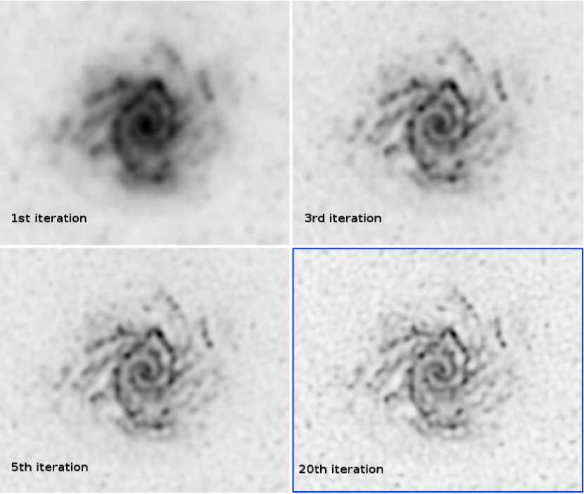
Figure 4.1: The HiRes ”flux” images for the PSW band (250 $\mu$m), for case 12 on NGC 628. The first, third, fifth and twentieth iterations are shown.

4.6.2 Processing of SPIRE maps

The HiRes method requires all input data to be well-conditioned, that is, to represent real signals on the sky. There cannot be any residual offsets in the timelines (as arise from the telescope background) and no artifacts such as glitches can be present. We ran the SPIRE destriper on the input data to produce Level 1 products with the signal levels normalized.

It is critical to this deconvolution method to subtract as much of the background as possible, without making the signals go negative. To optimize the background subtraction, the input and footprint-calculation stages were run in order to compute the global minimum of all the data. This minimum was then removed from all the data before proceeding with the rest of the HiRes processing. As a precaution against negative pixels causing problems with the deconvolution, any pixel values with negative flux were set to a value of $1\times 10^{-200}$ Jy/beam.

SPIRE maps are normally made onto pixel sizes of [6, 10, 14] arcseconds for the [250, 350, 500] $\mu$m bands. For the naive mapmaker used in the standard pipeline, smaller pixel sizes often lead to blank (NaN) values in the output maps. With HiRes it is possible to use smaller pixel sizes. The recommended sizes are half the standard values, that is, [3, 5, 7] arcseconds for the three SPIRE bands. For the mapmaking metrics the standard pixel sizes were used, except for one case including simulated sources for which the half-standard sizes were used. The Python version was employed for all calculations for the map-making workshop as the Java/HIPE version did not become available until early July 2013.

For each of the three bands, the same average beam profile was used as input to the method. Although the SPIRE beam has a small ellipticity, we did not try to match the rotation of the beam with the map, instead just assuming that the position angles were already matched. We used the average beam profiles that the SPIRE ICC derived from Neptune observations made on a 1-arcsecond pixel grid, needing only the central region of 71x71 pixels for 500 $\mu$m and 151x151 pixels for 250 $\mu$m and 350 $\mu$m. (N.B. the inconsistency of the sizes is an accident but it should not affect the HiRes results very much – the smaller size used for 500 $\mu$m was chosen by Frank Masci when running the ICORE deconvolution on another dataset.)

In the HiRes lexicon, a “footprint” is the beam profile laid down on the output grid for a given detector sample. In effect each footprint is the point response function (PRF) evaluated for a particular pixel phase. Calculations were made with the PRF sampling at 1 arcsecond for PSW, and 2 arcseconds for both PMW and PLW.

The correction was accelerated using the BOOST SQUARED option for iterations 2 to 5. This means that the correction factor was squared for these iterations.

The maps were processed with a 10-pixel boundary around the final desired image sizes. The boundary was trimmed from the 20th-iteration images to produce the final delivered maps.

4.7 SUPREME (Hacheme Ayasso)

4.7.1 Introduction

SUPREME is a super-resolution mapmaker destined for extended emission with integrated destriping capacities [2]. It is based on a realistic physical model and an unsupervised Bayesian approach which jointly estimate the map and other parameters of the model automatically from the data. Therefore, It is easy to use since no parameter is required from the user. However, it is also possible for the user to fix any of model parameters for fine tuning. The original code is developed in MATLAB^TM, and a Java plugin for HIPE [7] is available for the community since the beginning of 2013. This method is applied to SPIRE/Herschel, however it can be extended to other instruments. An implementation to PACS mapmaking is being investigated.

The method

SUPREME mapmaking approach is based on physical model which links the measurements $\mathbf{y}$ to the observed sky $\mathbf{x}$. For SPIRE, the observation model is given as

$$\mathbf{y}=\mathrm{H}\mathbf{x}+\mathbf{n}$$ (4.1)

where $\mathrm{H}$ is the instrument model and $\mathbf{n}$ is the measurement noise which can be modelled by a Gaussian distribution with a unknown variance $\rho^{-1}_{n}$ and an offset $\mathbf{o}$ to compensate for the thermal drift in the measurement. In the current implementation of SUPREME, the instrument model is limited to telescope pointing $\mathrm{P}$ and beam $\mathrm{C}$ [16] models. Therefore, the data $\mathbf{y}$ are considered to be corrected for all other instrumental effects which is the case of Level1 data.

Estimating the map $\mathbf{x}$ given $\mathbf{y}$ and $\mathrm{H}$ lacks a unique and a stable solution (ill posed problem) specially in a super-resolution context. Therefore, a prior information is needed for $\mathbf{x}$ to regularize the solution. SUPREME is designed for extended emission mapmaking, hence a Markov field favorizing sky smoothness is used as a prior. The degree of sky smoothness is controlled by a correlation parameter $\rho_{x}$ which is supposed unknown.

SUPREME handles the inference in a Bayesian framework where the high resolution map $\mathbf{x}$ and the other model parameters (hyper-parameters) $\boldsymbol{\theta}=\left\{\rho_{s},\rho_{n},\mathbf{o}\right\}$ are chosen to maximize the joint posterior distribution. However the Joint Maximum A Posteriori (JMAP) is intractable, the estimation is performed in an iterative scheme with an automatic stopping criteria. After the convergence, the map and the hyper-parameters are given with their confidence intervals thanks to the probabilistic approach. Furthermore, the Bayesian theory presents a flexible framework for fixing some of the hyper-parameters within a supervised estimation situation. Moreover, the high resolution mapmaking naturally changes the beam profile associate with the maps. The new beam profile, so called equivalent beam, is calculated directly from the instrument and the other model hyper-parameters. It has a flat spectral density for spatial scales where the signal is dominant and it decreases steeply for spatial scales where the noise is dominant (Figure.4.2).

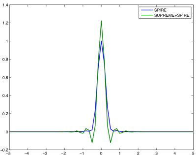
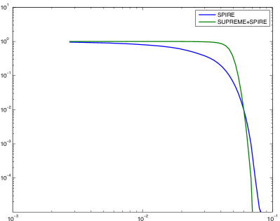
(a)	(b)

Figure 4.2: Comparison between instrument beam profile (SPIRE) and the high resolution equivalent beam profile (SPIRE+SUPREME). (a) the spatial representation, (b) spectral representation

Key features

• High resolution maps: The resolution gain is up 3 times compared to classical Coadd mapmakers

• Instrument beam model is included based on the work of Sibthorpe et al [16]. The user gets to select between the simulated and the empiric models.

• 2 telescope pointing models are available: nearest neighbor model (like the model used in HIPE mapmaker) and bilinear interpolation model. The latter is more accurate compared to the former, however it is more time consuming.

• A Gaussian noise model with variable offsets to achieve map destriping. The noise variance $\rho_{n}^{-1}$ and the offsets $\mathbf{o}$ can be estimated automatically or set by the user. The offsets are considered constant per leg per bolometer.

• A markovian model for the sky with a correlation parameter $\rho_{s}$ which can be estimated automatically or fixed by the user.

• The method provides also an error map and intervals of confidence for all the estimated variables as a byproduct thanks to the Bayesian framework.

• Controlled equivalent beam model: the expression of the equivalent beam model of the high resolution map is provided for users

4.7.2 Processing

SUPREME accepts level 1 inputs for high resolution mapmaking. Therefore, the plugin runs the standard HIPE pipeline to prepare data from level-0. However, it can accept directly level-1 data which are prepared with a non-standard pipeline. In an automatic estimation framework, the user chooses the beam, pointing and thermal drift models.

For benchmark data processing, the drift corrected data were used directly without any pre-treatment. The beam model was fixed to simulated one, the pointing model to a bilinear one and the drift model to constant per leg per bolometer. All other parameters were estimated automatically.

Example of performance

The following figure (Horsehead nebula) demonstrates the high resolution capacity of our method. These parameters were used

• pixel size = 3”,

• simulated beam,

• automatic estimation for noise and field variances,

• offset per leg per bolometer option,

• manual stopping condition with 500 iterations

More results are available in [2].

Figure 4.3: Reconstruction results for Horsehead nebula (real data Herschel). (a) Coadd map form instrument PACS ($70\mu m$) , (b) Coadd map from instrument SPIRE $250\mu m$, (c) Coadd map PACS ($160\mu m$), (d) SUPREME map from instrument SPIRE $250\mu m$

4.7.3 Comments

• Since the method is designed for extended emission , applying it to fields with high intensities point sources might generate ring artifacts around them which corresponds to the spatial response of equivalent beam. While this ringing effect is normal, it may make SUPREME maps less useful. Therefore, another method (SUPREMEX) was developed for joint mapmaking and source extraction. The scientific description of the method is given in Ayasso et al, [3]. It will be implemented soon into HIPE plugin.

• In certain fields where the detector offset variation is strong the maps might still contain some stripes. Therefore, an enhanced noise model is under development for a better destriping.

Chapter 5 Metrics and Results

The maps made by different map-makers are examined and compared in the framework of four sets of metrics:

(1) Deviation from the truth. These metrics are applied to maps of simulated test cases that are based on real MIPS 24$\mu m$ maps (simulated cases based on artificial sources are excluded). For these maps, deviations from the truth are the most direct and objective measures of the bias introduced by the map-making process. These metrics include:

• visual examinations of the difference maps ($\rm Map-Map_{true}$);

• scatter plots of (S – S_true) vs S_true for individual pixels;

• slopes of these plots;

• absolute deviations: mean and standard deviation of S – S_true;

• relative deviations: mean and standard deviation of (S – S_true)/S_true.

(2) Spatial (2-D) power spectra. These are powerful tools to characterize the spatial distributions of maps in a general and abstract manner. Comparisons between the power spectra of maps made by different map-makers and those of the truth maps can reveal biases introduced by map-making processes and by SPIRE instrumental noise (e.g. the “cooler burp”). These metrics include:

• power spectra plots

• plots of the divergence from the truth power spectrum, only for simulated cases.

(3) Point source and extended source photometry. These metrics, applying to the simulated test cases based on artificial sources (Cases 1, 5 and 8), are to test map-makers on their ability in handling point sources and extended source, in particular on how well they can preserve the fluxes in the map-making process. The metrics include:

• astrometry of point sources;

• point source and extended source photometry;

• detection rates of faint point sources, obtained using Starfinder (a point source extractor);

• point source beam profiles.

(4) Metrics for super-resolution maps. These metrics are applied to maps made by HiRes and SUPREME, the two super-resolution mappers, and compare them to maps made by the destriper (the pipeline default). They include:

• visual examinations of the maps;

• spatial power spectra;

• point source beam profiles.

Results of investigations using these metrics are presented in the following sections in this chapter, written by individuals who carried out these analyses.

5.1 Deviation from the truth – Difference maps (Vera Könyves & Andreas Papageorgiou)

5.1.1 Test Data

Only simulated test cases (case 2, 4, 6, 9, and 10) were used in this metrics as we need a ”truth” map from which the difference will be derived. This way we can measure the biases, introduced by the various map-making methods. In these tests we excluded the cases containing only artificial point/extended sources. The following table 5.1 shows the simulated data sets for this metrics. For simplicity, but to still give representative results, only the PSW/250 $\mu$m and PLW/500 $\mu$m maps were tested.

Case	Mode	Truth Layer	Noise Layer	Map Size	Depth	Maps
2	Nominal	cirrus region	Lockman-North	0.7d $\times$ 0.7d	7 repeats	PSW, PMW, PLW
4	Nominal	M51	Lockman-North	0.7d $\times$ 0.7d	7 repeats	PSW, PMW, PLW
6	Fast-Scan	Galactic center	Lockman-SWIRE	3.5d $\times$ 3.5d	7 repeats	PSW, PLW
9	Parallel	Galactic center	ELAIS N1	1.3d $\times$ 1.3d	7 repeats	PSW, PLW
10	Parallel	cirrus region	ELAIS N1	1.3d $\times$ 1.3d	7 repeats	PSW, PLW

Table 5.1: Simulated data sets used in the ”Difference map metrics”.

I also list here the availability of reprocessed maps which were compared to the above truth maps:

• Case 2, and 9: Naive, destriper/P0, destriper/P1, Scanamorphos, Sanepic

• Case 4: Naive, Naive with human intervention, destriper/P0, destriper/P1, Scanamorphos, Sanepic

• Case 6, and 10: Naive, destriper/P0, destriper/P1, Scanamorphos, Sanepic, Unimap

’P0’ and ’P1’ denotes the zero-, and first-order polynomial baseline removal in the HIPE destriper method.

The maps were on the same WCS grid with the same units, therefore no further preparation was needed before making the difference maps.

5.1.2 Analyses and Results

In this ”Deviation from the truth – Difference maps” metrics we present for each mapper method:

• a scatter plot of (S – S_true) vs S_true for individual pixels;

• slopes of these plots;

• absolute deviations: mean and standard deviation of S – S_true;

• relative deviations: mean and standard deviation of (S – S_true)/S_true;

IDL scripts were used to make difference maps, plots, and obtain statistics over the maps.

Case 2 (nominal cirrus)

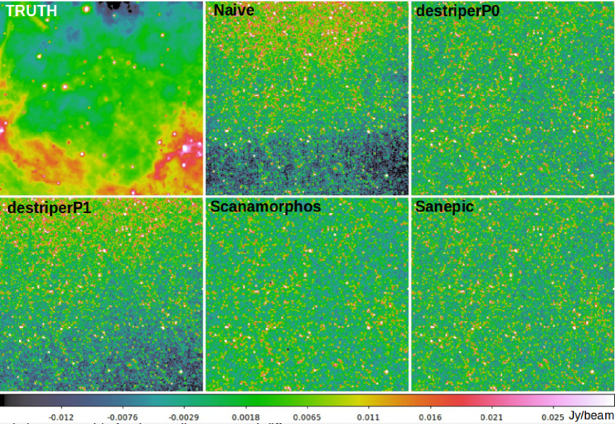
Figure 5.1: Truth and Difference maps for case 2, PSW (nominal cirrus). For the latter ones, (Diff – median(Diff)) is shown, therefore the Jy/beam scale is comparable for the median-removed difference maps.

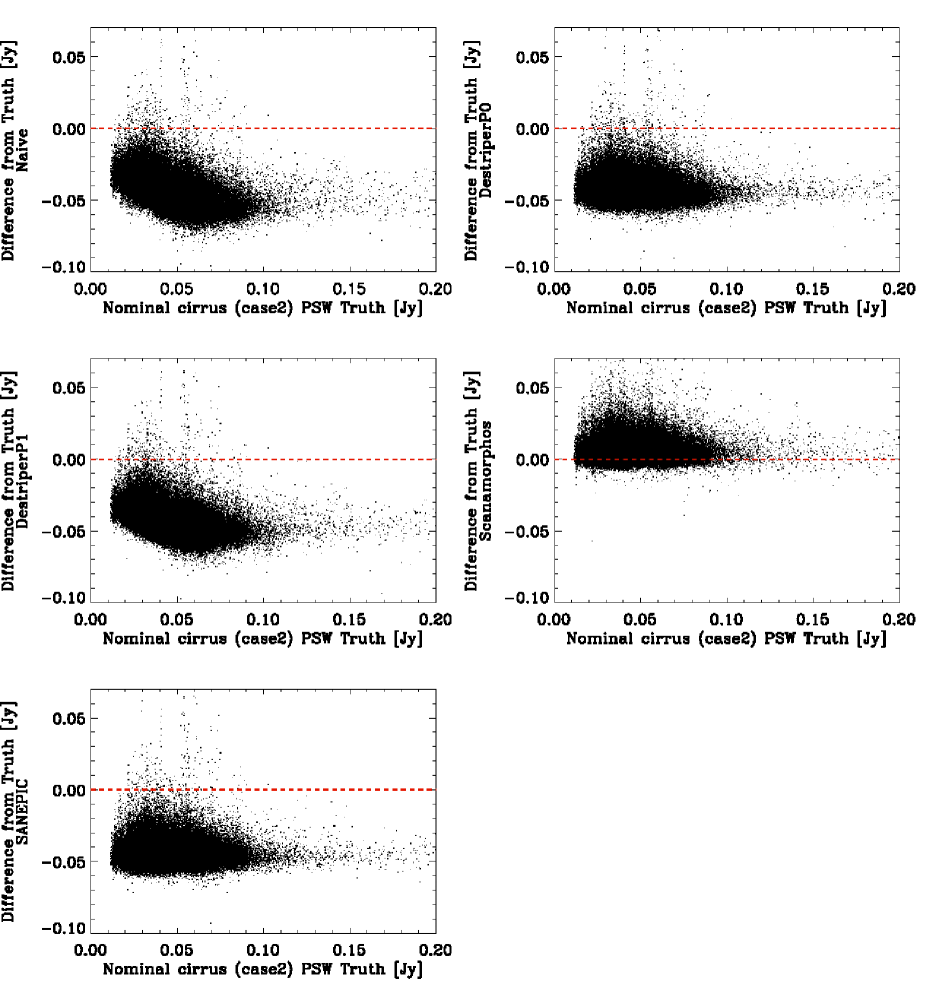
Figure 5.2: Scatter plots of the difference maps for case 2, PSW; (S – S_true) vs S_true.

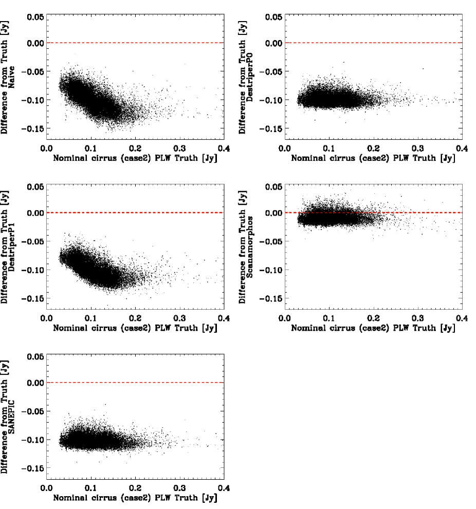
Figure 5.3: Scatter plots of the difference maps for case 2, PLW; (S – S_true) vs S_true.

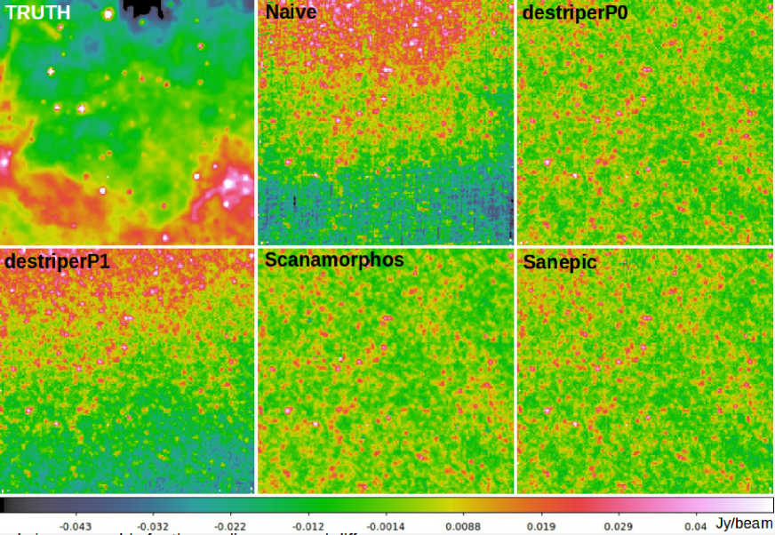
Figure 5.4: Truth and Difference maps for case 2, PLW (nominal cirrus). For the latter ones, (Diff – median(Diff)) is shown, therefore the Jy/beam scale is comparable for the median-removed difference maps.

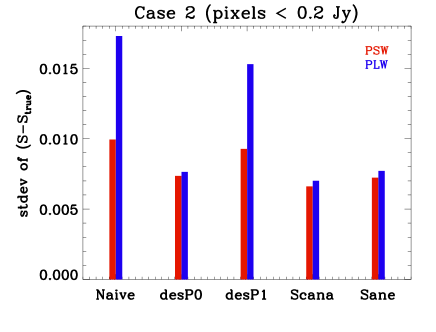
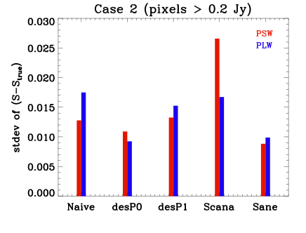
Figure 5.5: Standard deviation of the difference from the truth, for case 2, PSW (red) and PLW (blue) bands, separately for the S_true $<$ 0.2 Jy (faint), and S_true $>$ 0.2 Jy (bright) emission.

The case 2 difference maps of both bands show a gradient for the ’Naive’ and the ’destriperP1’ methods which may come from the oversubtraction of the bright emission of the truth image in the Southern part. In the ’Naive’ case a median baseline removal was applied; while a 1^st-order polynomial baseline fit in ’destriperP1’. The Naive map also produces stripy pattern due to a simpler median subtraction of the residual offsets from the different detectors. The gradients are visualized in the scatter plots as anticorrelation of the difference vs truth values. The other methods compensate for this effect. For example, with Scanamorphos, it is the /galactic option which takes into account the complexity of the field; the different amount of emission at the map edges.

Case 4 (nominal M51)

The case 4 difference map scatter plots are not so suggestive, as there are fewer map pixels; and their main feature is the vertical line, due to the observed data edges which was embedded in a very faint emission background. The median-removed difference maps are very homogeneous for almost all the mappers. The Naive mapper leaves over-subtracted bands in the scanning directions which disappears with human intervention, when a mask can be created over the central source to be left out in the baseline determination. The human intervention on the other hand introduces an artifact over the high dynamic range central source.

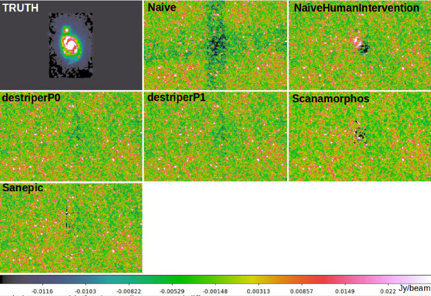
Figure 5.6: Truth and Difference maps for case 4, PSW (nominal M51). For the latter ones, (Diff – median(Diff)) is shown, therefore the Jy/beam scale is comparable for the median-removed difference maps.

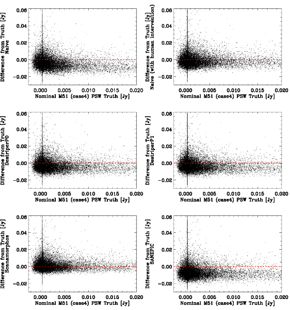
Figure 5.7: Scatter plots of the difference maps for case 4, PSW; (S – S_true) vs S_true.

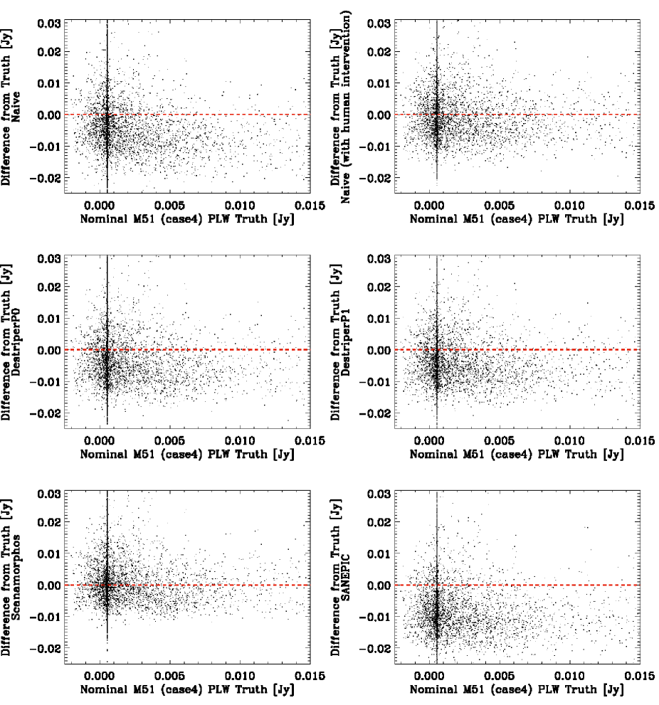
Figure 5.8: Scatter plots of the difference maps for case 4, PLW; (S – S_true) vs S_true.

Figure 5.9: Truth and Difference maps for case 4, PLW (nominal M51). For the latter ones, (Diff – median(Diff)) is shown, therefore the Jy/beam scale is comparable for the median-removed difference maps.

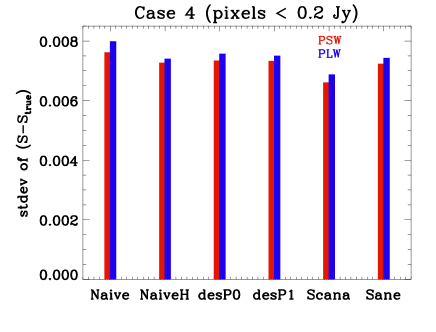
Figure 5.10: Standard deviation of the difference from the truth, for case 4, PSW (red) and PLW (blue) bands, separately for the S_true $<$ 0.2 Jy (faint), and S_true $>$ 0.2 Jy (bright) emission.

Case 6 (fast scan Galactic center)

Complex fields are more complicated, the difference maps can show various artifacts. With Destriper P0 and P1: either erroneous bolometers, scanning through bright data peaks, are leaving outlier scans in the resulting map, or this outlier baseline removal is due to the inability of the Destripers to deal with the SPIRE ”cooler-burps”.

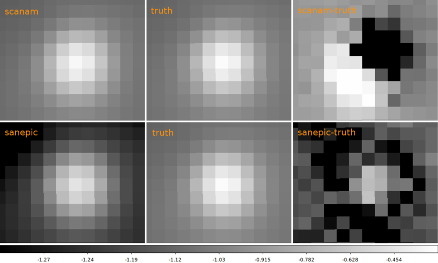
Figure 5.11: A case 6/PSW map detail in the processed Scanamorphos map (upper left), the truth map (middle), and the difference map from the truth (upper right). The same is given for Sanepic (lower panels) for comparison. All the maps are on the same grid.

The over-/under-subtraction in the Galactic plane, or an apparent positional offset(?) in the Scanamorphos difference map is very likely due to the fact that it slightly modifies the PSF. We must emphasize that this apparent positional offset in the difference map of Scanamorphos *does not* manifest itself (in the processed Scanamorphos maps) as sources projected off-center from the actual truth positions. This effect is visualized in Fig. 5.11. This was also confirmed by the true position offset checks of the Point and Extended Sources Photometry metrics.

Cross-like point source artifacts around bright sources can be well seen in the Sanepic PLW map. This is a typical feature of GLS (Generalized Least Square) approaches, possibly due to misalignment of the PSF with respect to the final projected sky grid. One method to remove them (P/WGLS routines – e.g., for Unimap) is described in Piazzo (2013), [13], but matching the scan and cross-scan directions with much better astrometric accuracy also mitigates this problem (Aussel et al., PACS-ICC investigations). In the difference map vs truth scatter plots, the Destripers are showing a surprisingly narrow distribution in the Galactic center cases (6, 9).

Figure 5.12: Truth and Difference maps for case 6, PSW (fast scan Galactic center). For the latter ones, (Diff – median(Diff)) is shown, therefore the Jy/beam scale is comparable for the median-removed difference maps.

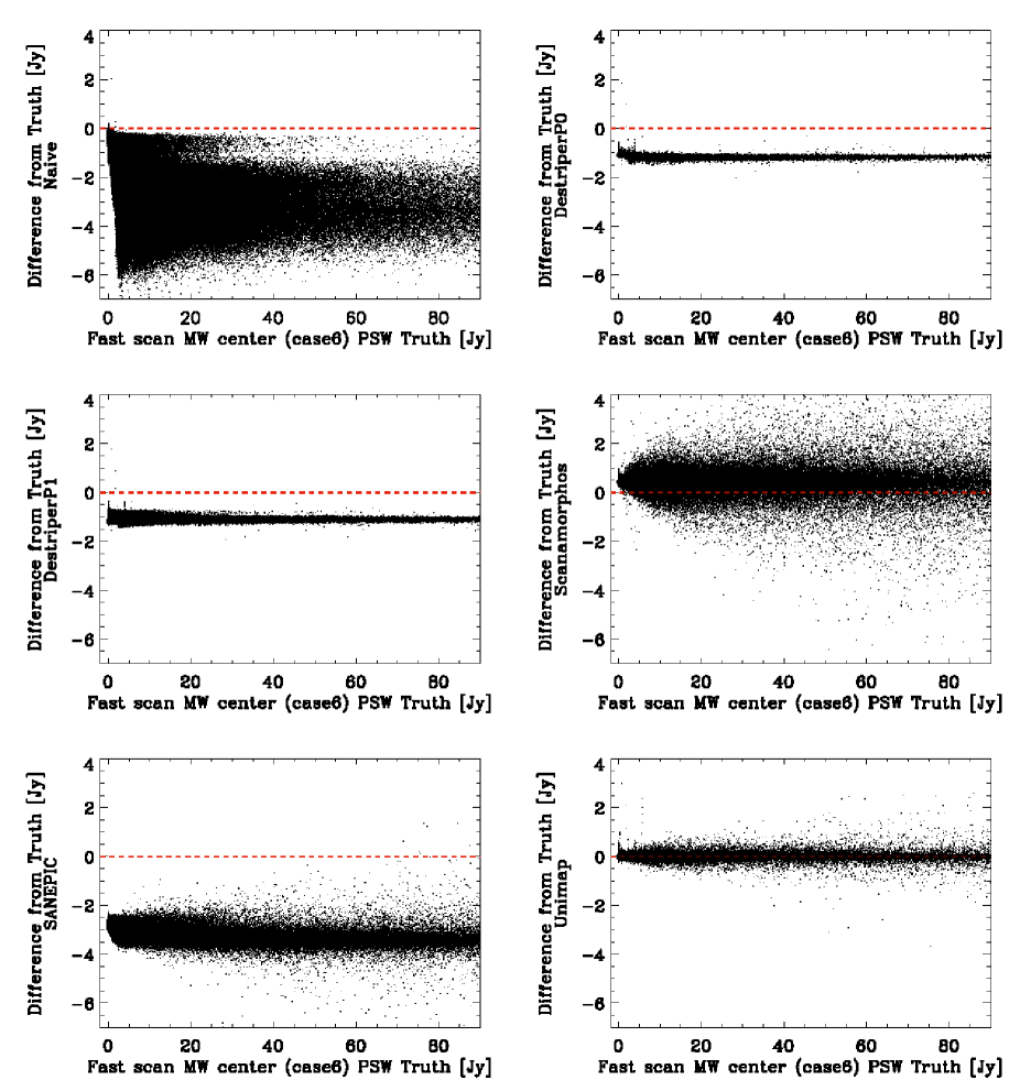
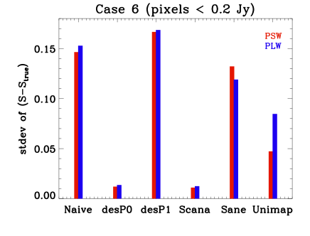
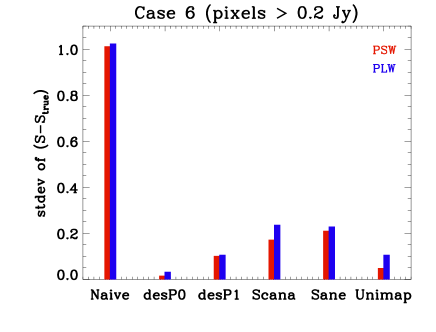
Figure 5.13: Scatter plots of the difference maps for case 6, PSW; (S – S_true) vs S_true.

Figure 5.14: Scatter plots of the difference maps for case 6, PLW; (S – S_true) vs S_true.

Figure 5.15: Truth and Difference maps for case 6, PLW (fast scan Galactic center). For the latter ones, (Diff – median(Diff)) is shown, therefore the Jy/beam scale is comparable for the median-removed difference maps.

Figure 5.16: Standard deviation of the difference from the truth, for case 6, PSW (red) and PLW (blue) bands, separately for the S_true $<$ 0.2 Jy (faint), and S_true $>$ 0.2 Jy (bright) domain.

Case 9 (parallel Galactic center)

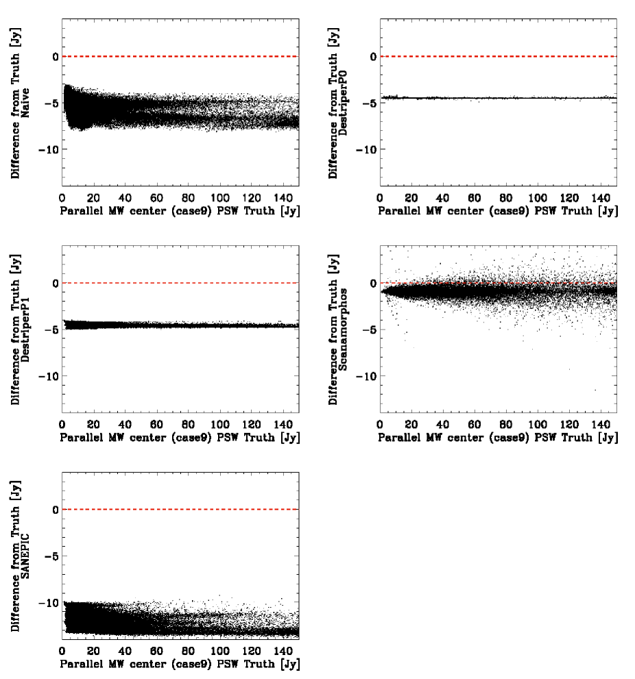
Figure 5.17: Scatter plots of the difference maps for case 9, PSW; (S – S_true) vs S_true.

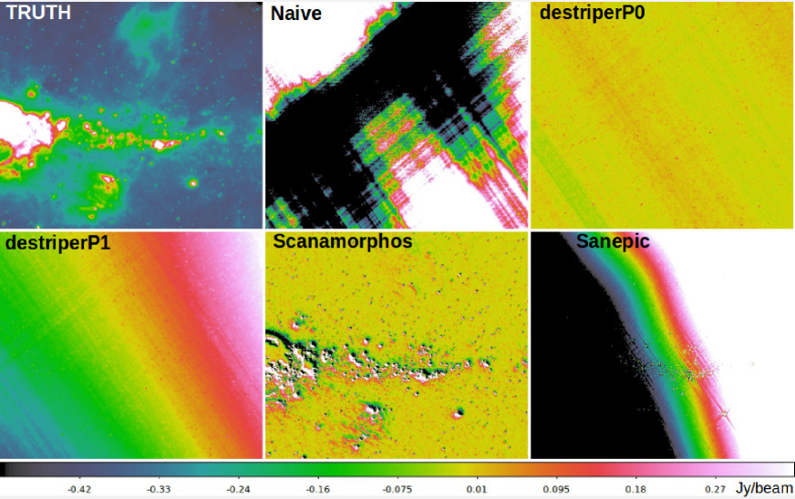
Figure 5.18: Truth and Difference maps for case 9, PSW (parallel Galactic center). For the latter ones, (Diff – median(Diff)) is shown, therefore the Jy/beam scale is comparable for the median-removed difference maps.

Figure 5.19: Standard deviation of the difference from the truth, for case 9, PSW (red) and PLW (blue) bands, for the S_true $>$ 0.2 Jy (bright) emission.

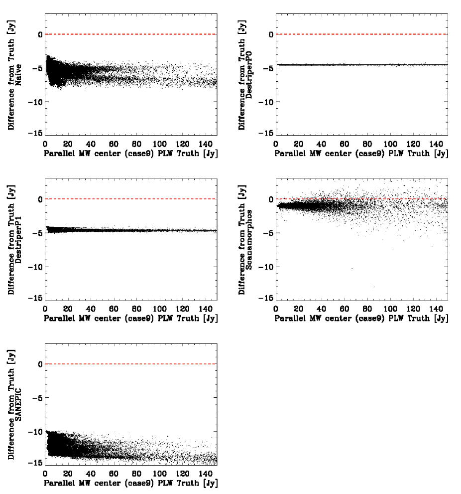
Figure 5.20: Scatter plots of the difference maps for case 9, PLW; (S – S_true) vs S_true.

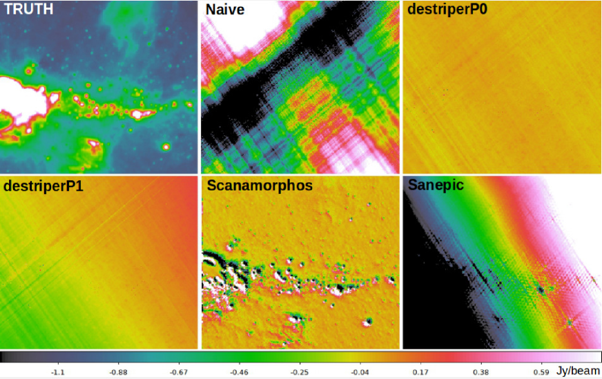
Figure 5.21: Truth and Difference maps for case 9, PLW (parallel Galactic center). For the latter ones, (Diff – median(Diff)) is shown, therefore the Jy/beam scale is comparable for the median-removed difference maps.

Observations, statements for case 6 maps are mostly true in this similar case 9 too (e.g., Sanepic, Scanamorphos, Destripers). In the Sanepic map the strong gradient likely originates from the mapper’s assumption that the data is circulant, while in this case, it is not. In Scanamorphos, it is the /galactic option which takes into account the non-circulant nature of the data. See these details again in the Summary/Conclusions.

Case 10 (parallel cirrus)

In this low dynamic range example the map makers produce very similar, and satisfactory results.

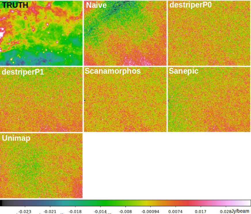
Figure 5.22: Truth and Difference maps for case 10, PSW (parallel cirrus). For the latter ones, (Diff – median(Diff)) is shown, therefore the Jy/beam scale is comparable for the median-removed difference maps.

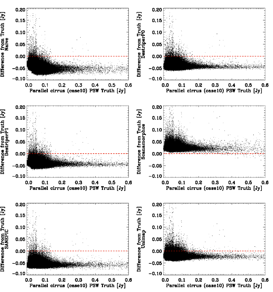
Figure 5.23: Scatter plots of the difference maps for case 10, PSW; (S – S_true) vs S_true.

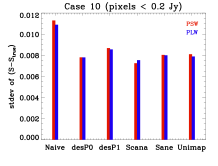
Figure 5.24: Standard deviation of the difference from the truth, for case 10, PSW (red) and PLW (blue) bands, separately for the S_true $<$ 0.2 Jy (faint), and S_true $>$ 0.2 Jy (bright) domain.

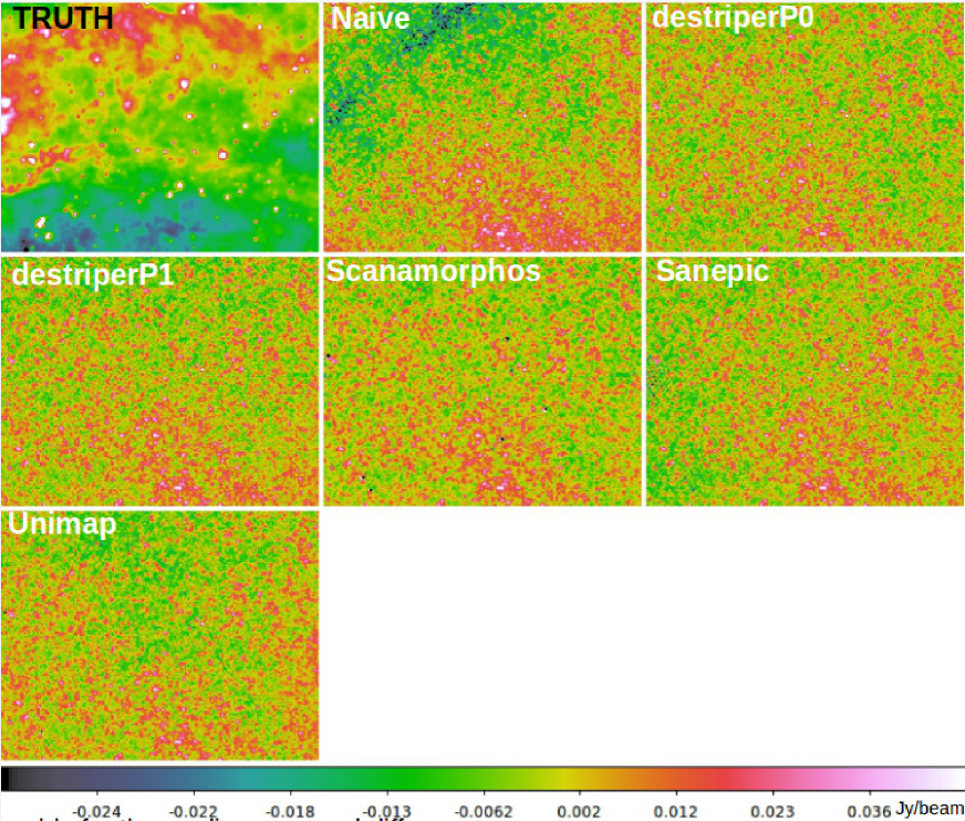
Figure 5.25: Truth and Difference maps for case 10, PLW (parallel cirrus). For the latter ones, (Diff – median(Diff)) is shown, therefore the Jy/beam scale is comparable for the median-removed difference maps.

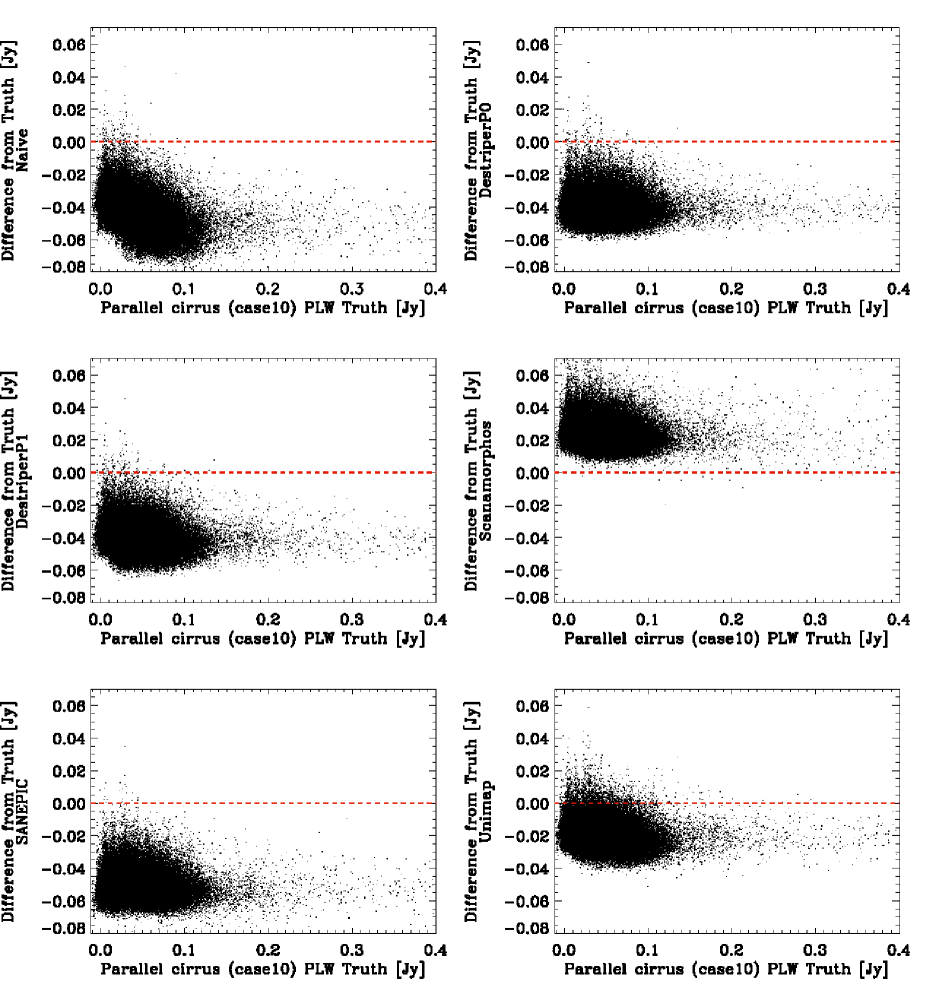
Figure 5.26: Scatter plots of the difference maps for case 10, PLW; (S – S_true) vs S_true.

5.1.3 More ’table’ results

	case 2				case 9
	PSW		PLW		PSW		PLW
	mean	stdev	mean	stdev	mean	stdev	mean	stdev
naive	-0.0429	0.0099	-0.0996	0.0174	-5.0302	0.8410	-5.0599	0.8436
destrP0	-0.0427	0.0073	-0.0991	0.0076	-4.5131	0.0131	-4.5184	0.0204
destrP1	-0.0429	0.0092	-0.0994	0.0153	-4.5192	0.1864	-4.5231	0.1840
scanam	0.0053	0.0066	-0.0094	0.0072	-0.9391	0.2353	-1.0083	0.3852
sanepic	-0.0445	0.0072	-0.1023	0.0077	-11.5947	0.9713	-11.8134	1.1405

	case 4
	PSW		PLW
	mean	stdev	mean	stdev
naive	-0.0017	0.0076	-0.0022	0.0080
naiveHuman	-0.0002	0.0074	-0.0002	0.0076
destrP0	-0.0017	0.0073	-0.0024	0.0075
destrP1	-0.0017	0.0073	-0.0025	0.0075
scanam	0.0017	0.0068	0.0013	0.0078
sanepic	-0.0059	0.0072	-0.0076	0.0075

	case 6				case 10
	PSW		PLW		PSW		PLW
	mean	stdev	mean	stdev	mean	stdev	mean	stdev
naive	-1.3883	1.0154	-1.4105	1.0264	-0.0463	0.0113	-0.0441	0.0109
destrP0	-1.1215	0.0153	-1.1357	0.0303	-0.0420	0.0078	-0.0403	0.0077
destrP1	-1.1149	0.1197	-1.1292	0.1235	-0.0421	0.0086	-0.0403	0.0085
scanam	0.4073	0.1546	0.3911	0.2138	0.0221	0.0090	0.0235	0.0173
sanepic	-3.0149	0.2215	-3.0339	0.2294	-0.0545	0.0080	-0.0507	0.0080
unimap	-0.0008	0.0493	-0.0211	0.1042	-0.0219	0.0081	-0.0201	0.0079

Table 5.2: Absolute deviations: mean and standard deviation of (S - S_true). Results are shown for cases 2, 4, 6, 9, and 10, for the available map makers.

The slopes of the difference map scatter plots were obtained as coeff(1) of the IDL’s robust_linefit routine, and their errors were normalized by the map pixels (csig(1)*sqrt(N)). This is provided for the S_true $>$ 0.2 Jy domain and shows if a map-maker introduces any bias for the bright pixels. This is visualized in the scatter plot figures for each case and PSW/PLW bands.

	case 2				case 9
	PSW		PLW		PSW		PLW
	mean	stdev	mean	stdev	mean	stdev	mean	stdev
naive	-1.0752	0.3474	-1.0656	0.2999	-0.9479	0.5620	-0.9466	0.5611
destrP0	-1.1168	0.4647	-1.1100	0.4363	-0.9051	0.5889	-0.8995	0.5852
destrP1	-1.0804	0.3586	-1.0706	0.3109	-0.8977	0.5678	-0.8923	0.5646
scanam	0.1383	0.1841	-0.1078	0.0957	-0.1873	0.1220	-0.1979	0.1290
sanepic	-1.1680	0.4943	-1.1426	0.4435	-2.2767	1.4251	-2.2901	1.4241

	case 4
	PSW		PLW
	mean	stdev	mean	stdev
naive	-3.1237	103.5528	-2.3820	163.2418
naiveHum	-0.5859	108.5850	0.2562	181.8850
destrP0	-3.8805	107.0133	-3.2674	152.9565
destrP1	-3.9140	107.1141	-3.4283	141.3440
scanam	4.1419	91.5670	2.9724	160.8298
sanepic	-13.9558	118.2347	-12.3324	94.6355

	case 6				case 10
	PSW		PLW		PSW		PLW
	mean	stdev	mean	stdev	mean	stdev	mean	stdev
naive	-1.8433	4256.5560	-7.0235	4394.7150	-0.9807	457.3350	-1.8878	111.8000
destrP0	-0.7295	7248.2743	-14.1292	9185.9890	-0.9219	489.7473	-1.9283	125.8154
destrP1	-1.0635	6151.4683	-12.9828	8145.7430	-0.9116	439.8811	-1.8479	117.9252
scanam	0.5090	2579.5553	5.0161	3218.3239	0.6074	237.1912	1.2517	91.1021
sanepic	-2.4014	18275.315	-35.7553	22986.732	-1.2562	588.3852	-2.5008	176.5462
unimap	0.2322	398.8190	0.2143	435.0549	-0.4689	247.9541	-0.8593	48.8528

Table 5.3: Relative deviations: Table of mean and standard deviations of (S - S_true)/S_true. Results are shown for cases 2, 4, 6, 9, and 10, for the available map makers.

	case 2				case 9
	PSW		PLW		PSW		PLW
	slope	slopeErr	slope	slopeErr	slope	slopeErr	slope	slopeErr
naive	0.0062	0.0331	0.0660	0.1179	-0.007826	0.022550	-0.007985	0.023011
destrP0	-0.0018	0.0159	0.0044	0.0574	-0.000038	0.000333	-0.000045	0.000550
destrP1	0.0044	0.0271	0.0429	0.0975	-0.001122	0.005092	-0.000983	0.005104
scanam	-0.0409	0.0497	-0.0265	0.0918	0.000007	0.000723	-0.000091	0.001560
sanepic	0.0030	0.0239	0.0081	0.0679	-0.009294	0.025961	-0.014845	0.029227

	case 4
	PSW		PLW
	slope	slopeErr	slope	slopeErr
naive	-0.0010	0.0096	-0.0030	0.0146
naiveHum	0.0091	0.0305	0.0044	0.0339
destrP0	-0.0007	0.0096	-0.0023	0.0140
destrP1	-0.0007	0.0096	-0.0023	0.0140
scanam	-0.0065	0.0250	-0.0131	0.0497
sanepic	-0.0004	0.0144	-0.0049	0.0264

	case 6				case 10
	PSW		PLW		PSW		PLW
	slope	slopeErr	slope	slopeErr	slope	slopeErr	slope	slopeErr
naive	-0.119569	0.147264	-0.123366	0.148822	-0.000459	0.005589	-0.001415	0.007617
destrP0	-0.000056	0.000652	-0.000092	0.000924	0.000046	0.003197	-0.000215	0.004927
destrP1	0.000323	0.005220	0.000114	0.005612	0.000103	0.003505	-0.000193	0.005307
scanam	0.001072	0.002506	0.001435	0.003560	-0.009363	0.013734	-0.019243	0.028724
sanepic	-0.014426	0.025079	-0.017577	0.022181	0.001269	0.005870	-0.011593	0.010348
unimap	-0.000036	0.002143	0.000329	0.004832	-0.000420	0.004908	-0.003886	0.008665

Table 5.4: Slopes and errors of the difference map scatter plots, calculated only for the S_true $>$ 0.2 Jy range.

5.1.4 Summary

We can draw a general conclusion: The data treatment is not optimal if the map-maker’s hypothesis does not meet the conditions of the simulations. For example, Sanepic in case 9, where the data is not circulant.

Further conclusions in the low dynamic range cases (2, 4, 10):

• Destriper/P0, Scanamorphos, and Sanepic produce similar results.

• By running Scanamorphos with the /galactic option (which preserves large scales) the residual slope is avoided, and the Scanamorphos scatter plots are comparable to the Sanepic and Destriper/P0.

• By running the Destriper with a 1st order polynomial baseline removal, residual slope will be introduced in the map.

In high dynamic range cases (6, 9):

• Destriper/P1, Sanepic, Unimap introduce different types of large spatial scale noise.

• Destriper/P0 avoids introducing large spatial scales.

  However, for specific scans the baseline is not properly removed, due to the inability of the Destriper/P0 (and P1 too) to deal with the SPIRE ”cooler-burps”?

• Scanamorphos also avoids introducing any large spatial scale noise.

  However, the scatter plots still display larger standard deviation, likely due to a slight positional offset introduced by the mapper (e.g., Scanamorphos difference maps, Case 9, PLW), and a slight change in the beam size.

5.2 Power Spectra (Luca Conversi)

5.2.1 Test Data

Five simulated test cases (cases 2, 4, 6, 9, 10) and five real cases (cases 3, 7, 11, 12 and 13) were examined in this metric. Tab. 5.5 lists the content of the different simulated cases. Cases 3, 7, and 11 are real SPIRE maps of extragalactic dark fields observed in different modes (SPIRE-only or parallel, slow or fast scan speed). Case 12 is a real SPIRE large map observation of NGC-628 taken at nominal scan speed, while case 13 is a Parallel mode observation of a Hi-Gal field taken at fast scan speed.

Case	Mapping Mode	Extended Layer
2	Nominal	24 micron cirrus
4	Nominal	M51
6	Fast scan	24 micron Galactic Centre
9	Parallel	24 micron Galactic Centre
10	Parallel	24 micron cirrus

Table 5.5: List of the different simulated cases.

Fig. 5.27 shows all the combinations between cases to be analyzed and available maps produced with different map-makers:

Truth

means that the input, noise-free map was available. Clearly, only cases with simulated extended data had such maps. N.B.: all truth maps are meant as simulated only data (no noise) but convolved with the instrument’s beam and reprojected on standard SPIRE pixel sizes (6 to 14 arcsec).

Naïve

are cases reduced with the standard HIPE median baseline subtraction plus naïve map-maker: all cases were available.

Naïve IA

are cases reduced in interactive analysis, where the user selected a suitable polynomial baseline removal and then ran the naïve map-maker: only cases 4, 7, 11 and 12 were available.

Destriper P0 and P1

are cases reduced with the HIPE destriper, using either a polynomial order of 0 or 1: all cases were available.

Scanamorphos

maps were available for all cases; however case 13 had a different WCS (maps were larger) in respect to the other map-makers maps, so a direct comparison of the power spectra was not possible (see Figs. 5.37 and 5.44).

Sanepic

maps were available only for the simulations, hence cases 12 and 13 were missing.

Unimap

maps instead were available only for cases 6, 10 and 12. Case 13 had different WCS (larger maps).

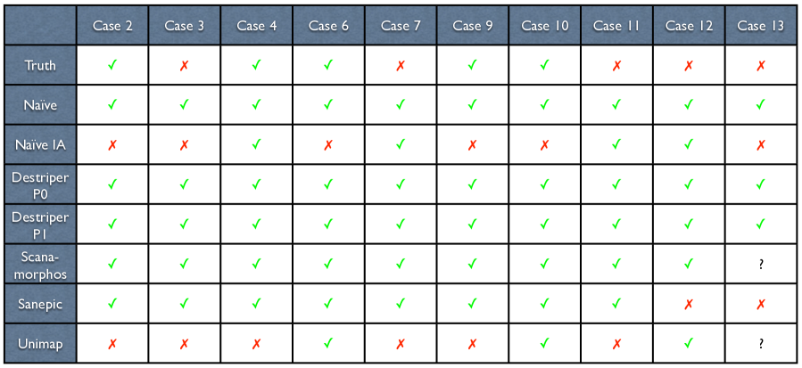
Figure 5.27: List of cases reduced with different map-makers: green marks mean maps for a given case/map-maker combination was available; red crosses indicate data was not reduced with the selected map-maker; a question mark indicates the cases were maps were available but had a different WCS in respect to the others, making more difficult a direct comparison of the power spectra.

5.2.2 Analyses and Results

The analysis is based on an IDL script kindly provided by Jim Ingalls.

1. It computes the inverse 2D fast Fourier transform of the input map, normalizing to the total surface brightness of the image, hence the importance of having maps with same WCS.

2. Then it creates a map of angular scale bins $k$, depending on map s size and resolution.

3. The average value in each $k$ bin is computed.

4. Finally, the power spectra $P(k)$ results are fitted between $k=[0.01,1]$ acrmin^-1

For the cases where a truth map was available, its power spectrum was used as benchmark. We defined the divergence as:

$$\Delta(k)=\frac{|P_{\it Map-maker}(k)-P_{\it Truth}(k)|}{P_{\it Truth}(k)}$$ (5.1)

Given the amount of data and plots, we will discuss only some cases. Results obtained on the cases not discussed are reported in Appx 5.2.4.

Case 2

Results of power spectra for case 2 (nominal speed, SPIRE-only scan map with simulated cirrus emission, see Tab. 5.5) are shown in Fig. 5.29 for PSW and in Fig. 5.30 for PLW: the power spectra computed on available maps are reported in Fig. 5.30a, while Fig. 5.30b shows the divergence from the truth power spectrum of the various map-makers.

From these plots it is evident how the naïve map-maker is higher than the others at small scales ($k>1$ arcmin^-1). Also, Sanepic and the two HIPE destriper flavors P0 and P1 agree very nicely, being the closer to the truth power spectrum at large scales ($k<0.2$ arcmin^-1). Finally, Scanamorphos is the map-maker giving the lowest power spectrum at small scales (i.e. closer to the truth power spectrum).

A more detailed analysis of the PSW power spectra is discussed in later sections.

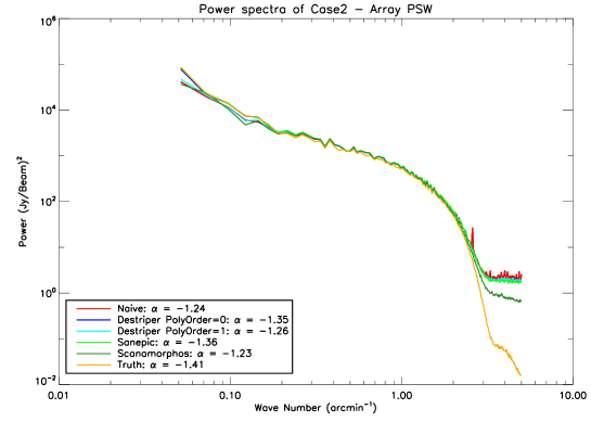
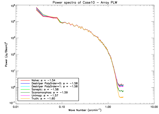
Figure 5.28: Results of power spectra for case 2 (see Tab. 5.5), PSW map: nominal speed, SPIRE-only scan map with simulated cirrus emission.

Figure 5.29: Results of power spectra for case 10 (see Tab. 5.5), PLW map: parallel mode observation with simulated cirrus emission.

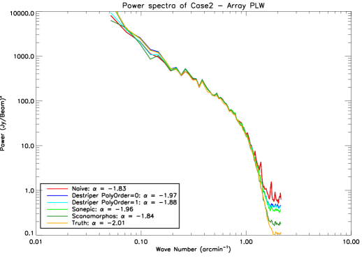
(a) Power spectra of PLW map

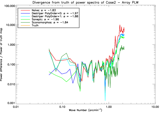
(b) Divergence from truth of PLW map power spectra

Figure 5.30: Results of power spectra for case 2 (see Tab. 5.5), PLW map: nominal speed, SPIRE-only scan map with simulated cirrus emission. In Fig. 5.30a the power spectra computed on available maps are reported, while Fig. 5.30b shows the divergence between the power spectrum computed on the truth map and the others.

Case 10

Results of power spectra for case 10 (parallel mode observation with simulated cirrus emission, see Tab. 5.5) are shown in Fig. 5.29b for PLW and in Fig. 5.31 for PSW: the power spectra computed on available maps are reported in Fig. 5.31a, while Fig. 5.31b shows the divergence from the truth power spectrum by the others.

Results are similar to the case 2 analysed earlier: the naïve map-maker is slightly higher than the others at small scales, but the general agreement among map-makers is good (within few percent). The only exemption is the Scanamorphos map-maker, which has the lowest power spectrum at small scales and being again closer to the truth power spectrum: this may be due Scanamorphos reproduction algorithm, which effectively smoothes the image (and hence the noise as well).

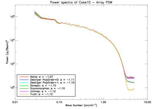
(a) Power spectra of PSW map

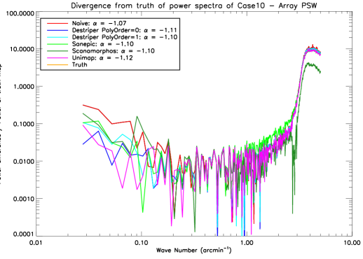
(b) Divergence from truth of PSW map power spectra

Figure 5.31: Results of power spectra for case 10 (see Tab. 5.5), PSW map: nominal speed, SPIRE-only scan map with simulated cirrus emission. In Fig. 5.31a the power spectra computed on available maps are reported, while Fig. 5.31b shows the divergence between the power spectrum computed on the truth map and the others. Also worth noting that Destriper P0 and Unimap are performing best at large scales ($k<0.2$ arcmin^-1), being closest to the truth power spectrum.

Cases 6 & 9

Results of power spectra for cases 6 (fast scan speed, SPIRE-only scan map with simulated galactic centre emission) and 9 (parallel mode observation with simulated galactic centre emission, see Tab. 5.5) are discussed together because they show the same behavior, being the sky signal really strong and much higher than the noise.

Fig. 5.32a and Fig. 5.33a present the power spectra computed on available PSW maps, for cases 6 and 9, respectively. The divergences of map-maker power spectra from the truth are reported in Figs. 5.32b and 5.33b.

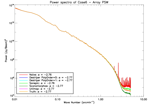
(a) Power spectra of PSW map

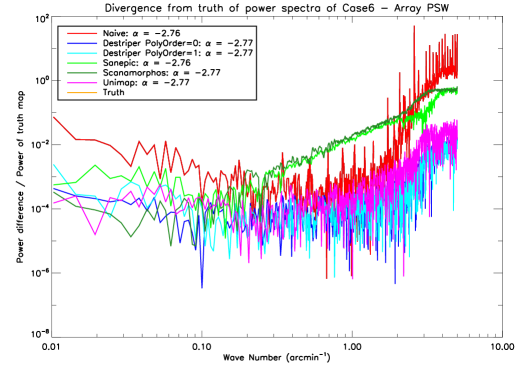
(b) Divergence from truth of PSW map power spectra

Figure 5.32: Results of power spectra for case 6 (see Tab. 5.5), PSW map: fast scan speed, SPIRE-only scan map with simulated galactic centre emission. In Fig. 5.32a the power spectra computed on available maps are reported, while Fig. 5.32b shows the divergence between the power spectrum computed on the truth map and the others.

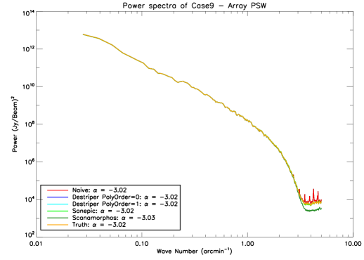
(a) Power spectra of PSW map

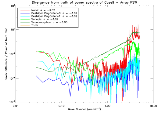
(b) Divergence from truth of PSW map power spectra

Figure 5.33: Results of power spectra for case 9 (see Tab. 5.5), PSW map: parallel mode observation with simulated galactic centre emission. In Fig. 5.33a the power spectra computed on available maps are reported, while Fig. 5.33b shows the divergence between the power spectrum computed on the truth map and the others. Again, Destriper P0 is the closest to the truth power spectrum at large scales ($k<0.2$ arcmin^-1).

As already mentioned, the sky signal is dominated by the galactic centre emission: as a consequence, all map-makers agree really well with the truth at all but small scales ($k>3$ arcmin^-1). Here, the naïve map-maker power spectrum is again higher than the others; it also presents a lot of peaks due to the leftover stripes: these are produced by the median baseline subtraction, an inadequate method given the high dynamic range of the present in the data. Also the Sanepic power spectrum is higher than the truth but to a lower extent. Again, Scanamorphos is giving a power spectrum which is lower than all the others, but this time even lower then the truth one.

The two HIPE destriper flavors P0 and P1 and the Unimap power spectra agree very nicely with the truth power spectrum, having a divergence of $10^{-3}\div 10^{-2}$, i.e. $\sim$2 orders of magnitude lower than the other map-maker power-spectra.

Case 7

Case 7 is a noise-only, fast scan speed, SPIRE-only scan map (see Tab. 5.5). The original SPIRE data contained a so-called cooler burp, i.e. the observation has been taken in the first 8h after a cooler recycle, where the cooler temperature is particularly unstable and the current pipeline is not capable to correct for the induced effects. Since there is no simulated signal added, the power spectra evidence the capabilities of the different map-makers to cope with such effect.

Fig. 5.34 reports the results for the PLW array: Fig. 5.34a is the full range, while Fig. 5.34b shows a zoom-in at small scales ($k>1$ arcmin^-1). Fig. 5.35 is the same for the PSW maps. From the plots, it is possible to deduce that:

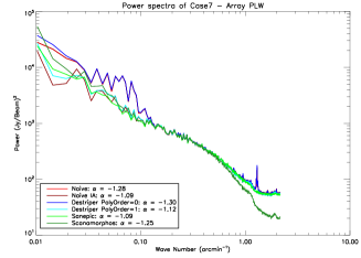
(a) Power spectra of PLW map

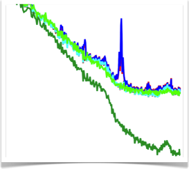
(b) Zoom-in of PLW maps power spectra

Figure 5.34: Results of power spectra for case 10 (see Tab. 5.5), PLW map: noise-only, fast scan speed, SPIRE-only scan map. In Fig. 5.34a the power spectra computed on available maps are reported, while Fig. 5.34b shows a zoom-in at small scales ($k>1$ arcmin^-1).

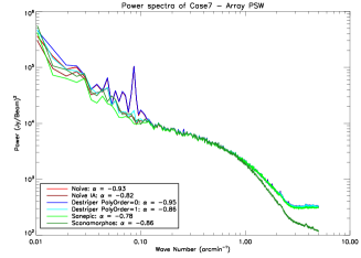
(a) Power spectra of PSW map

(b) Zoom-in of PSW maps power spectra

Figure 5.35: Results of power spectra for case 10 (see Tab. 5.5), PSW map: noise-only, fast scan speed, SPIRE-only scan map. In Fig. 5.35a the power spectra computed on available maps are reported, while Fig. 5.35b shows a zoom-in at small scales ($k>1$ arcmin^-1).

• The naïve map-maker and destriper with zero-th polynomial order are higher at large scales: this is a clear consequence that none of them was designed to correct for the cooler burp. Allowing a higher polynomial order fit solves the problem, as evidenced by the power spectra of Naïve IA and Destriper P1 map-makers, which are in perfect agreement with the others.

• PLW maps generated by Naïve and Destriper P0 map-makers also present a peak at $k\simeq 1.5$ (see Fig. 5.34b), which is not present in the PSW maps (see Fig. 5.35b): its origin is still unclear, but most probably related to the cooler burp too as it is not visible in any other case.

• The power spectrum obtained from Scanamorphos maps is again lower than the other spectra, while Sanepic, Naïve IA and Destriper P1 agree at all scales.

Case 12 & 13

Case 12 is the only real observation of which we have power spectra produced with all map-makers but Sanepic (see Fig. 5.27): in fact, maps of case 13 reduced with Scanamorphos are bigger and have a different WCS, making the power spectra comparison not straightforward.

Case 12’s power spectra results for the PMW array are shown in Fig. 5.37a, with a zoom-in at small scales ($k<1$ arcmin^-1) reported in Fig. 5.37b. Results for PLW and PSW are reported in Appx 5.2.4 (see Fig. 5.44). Results are similar to the other cases previously discussed: all map-makers agree very well at large scales, while at small scales Scanamorphos is lower than the others. Among them, Destriper P0, P1 and Naïve IA are almost identical, whereas Unimap and Naïve IA are slightly lower and higher, respectively.

Fig. 5.37a reports the case 13’s power spectra results for the PLW array, with a zoom-in at small scales ($k>1$ arcmin^-1) reported in Fig. 5.37b. At small scales, the Naïve map-maker spectrum presents peaks: these are due to the residual stripes in the maps, produced by the inadequate median baseline subtraction for the high dynamic range of the Hi-gal fields.

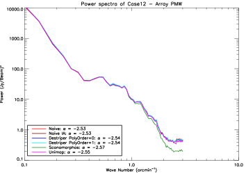
(a) Power spectra of PMW map

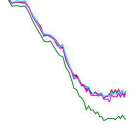
(b) Zoom-in of PMW maps power spectra

Figure 5.36: Results of power spectra for case 12, PMW map: real SPIRE-only large map observation of NGC-628 taken at nominal scan speed. In Fig. 5.37a the power spectra computed on available maps are reported, while Fig. 5.37b shows a zoom-in at small scales ($k>1$ arcmin^-1).

(a) Power spectra of PLW map

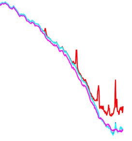
(b) Zoom-in of PLW maps power spectra

Figure 5.37: Results of power spectra for case 13, PLW map: real Parallel mode observation of a Hi-Gal field taken at fast scan speed. In Fig. 5.37a the power spectra computed on available maps are reported, while Fig. 5.37b shows a zoom-in at small scales ($k>1$ arcmin^-1).

5.2.3 Summary

Most of the power spectra, either coming from real or simulated data, noise-only or with extended emission, show very similar results.

• In the “central part” ($k=[0.1,1]$ arcmin^-1), results among different map-makers vary little: $\sim 1\%$ for cases where a truth map was available as benchmark.

• Differences with reference to truth map increase at $k>1$ arcmin^-1:

  • HIPE destripers with zero-th and first polynomial order, Sanepic and Unimap results are always very close;

  • Scanamorphos is usually lower;

  • The automatic HIPE Naïve mapper produces power spectra higher than the other map-makers, but in most cases (i.e. where the field dynamic range is not too high for the median baseline subtraction) it produced reasonable results. Spikes present in some cases at small scales (see e.g. Figs. 5.32, 5.33 and 5.37) are due to leftover stripes in the image. Moreover, once the Naïve mapper is ran in interactive analysis using a higher polynomial order fit for baseline removal, it gave results in line with other map-makers.

• At large scales ($k<0.2$ arcmin^-1), the spread among map-makers is larger, being the Destriper P0 and Unimap usually closer to the truth power spectrum.

• Case 7 (noise-only map with cooler burp, see Tab. 5.5) is a case apart:

  • Naïve and Destriper P0 map-makers perform worse: their power spectra are much higher at $k<0.1$ and present a peak at $k\sim 1.5$ in PLW map. This is to be expected as they cannot correct the drift caused by the cooler burp.

  • The other map-makers are in agreement, with Scanamorphos being lower at small scales.

5.2.4 Appendix: Power spectra of cases not discussed

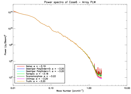
Figure 5.38: Results of power spectra for case 6, PLW map.

(a) Power spectra of PLW map

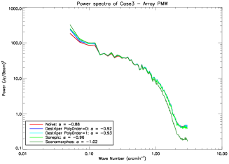
(b) Power spectra of PMW map

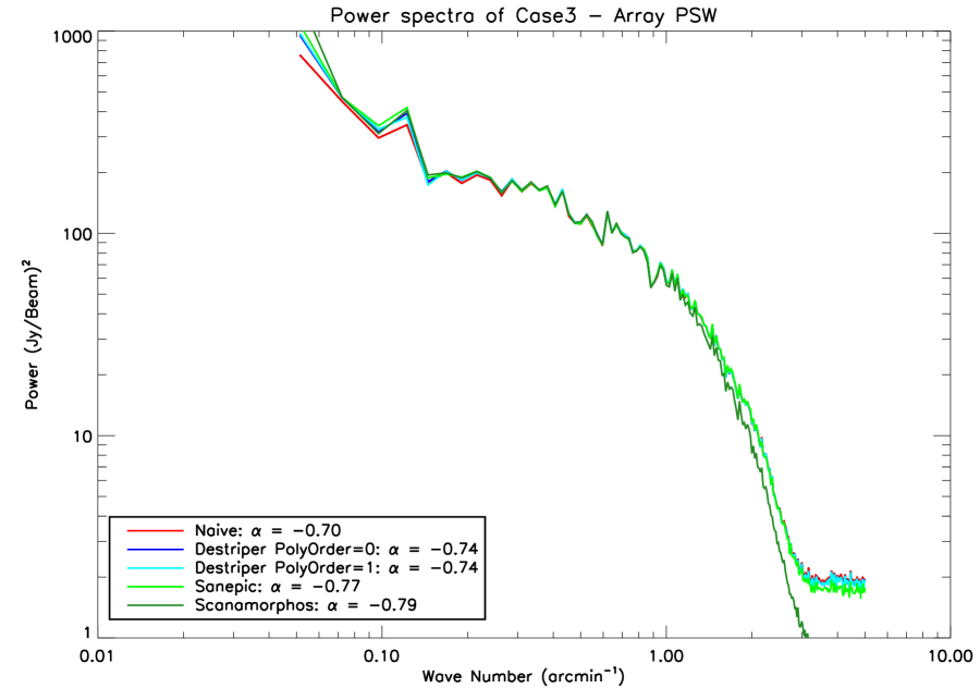
(c) Power spectra of PSW map

Figure 5.39: Results of power spectra for case 3.

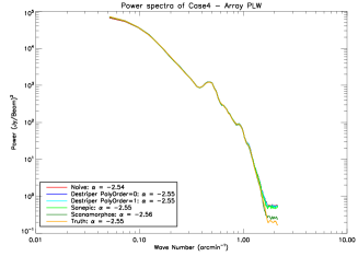
(a) Power spectra of PLW map

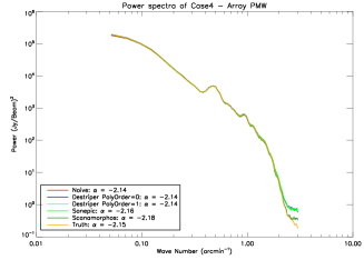
(b) Power spectra of PMW map

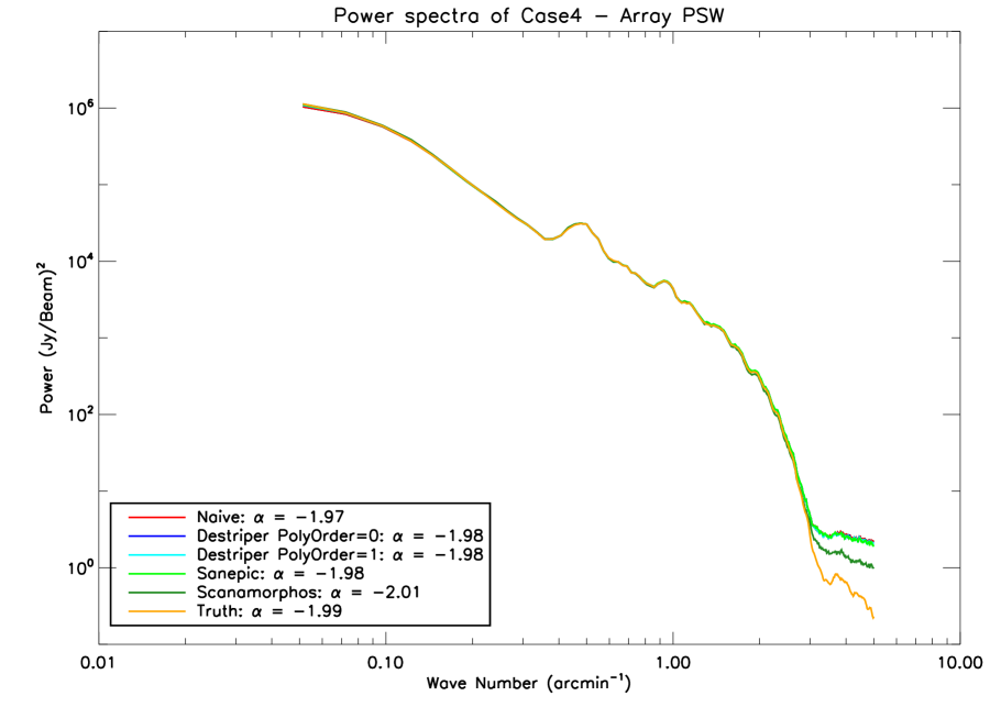
(c) Power spectra of PSW map

Figure 5.40: Results of power spectra for case 4.

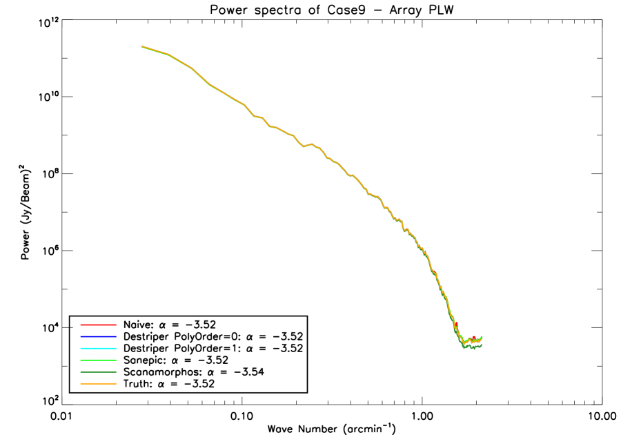
Figure 5.41: Results of power spectra for case 9, PLW map.

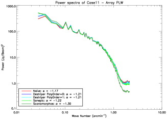
(a) Power spectra of PLW map

(b) Power spectra of PSW map

Figure 5.42: Results of power spectra for case 11.

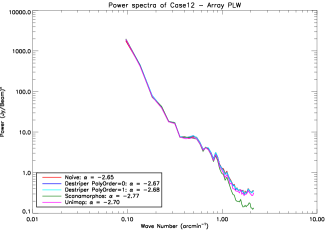
(a) Power spectra of PLW map

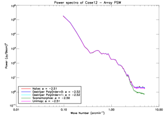
(b) Power spectra of PSW map

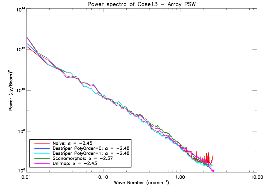
Figure 5.43: Results of power spectra for case 12.

Figure 5.44: Results of power spectra for case 13, PSW map. Note that Unimap and Scanamorphos power spectra have been multiplied by 0.2 to be aligned with the others.

5.3 Point Source and Extended Source Photometry (Kevin Xu)

5.3.1 Test Data

Three simulated test cases (Cases 1, 5 and 8; see Table 4.1) were examined in this metric. Four map-makers (Naive, Destriper-P0/Destriper-P1, Scanamorphos, SANEPIC) produced maps for all the three test cases. Unimap made maps for two test cases (Cases 1 and 5).

The Case 1 simulation (Fig. 5.45) is for the nominal mode. In the map of each of the three SPIRE bands, the simulation injected into the dark field observation (coverage $\rm=0.7\times 0.7$ deg²) 8 bright point sources (f=300 mJy), 8 faint point sources (f=30 mJy), and one extended source in the map center . The point sources were simulated using the observed PSF of the given band. The extended source (fpeak = 1 Jy/beam) is modeled as an exponential disk with the e-folding radius of 90 arcsec before being convolved with the PSF.

Figure 5.45: Truth map of Case 1 (nominal mode, $\rm 0.7\times 0.7$ deg²); in the PLW band.

In both Case 5 simulation for the fast-scan mode (coverage=3.5 × 3.5 deg2, Fig. 5.46a) and Case 8 simulation for the parallel mode (coverage=1.4 × 1.4 deg2, Fig. 5.46b), there are 36 bright sources (f=300 mJy), 36 faint sources (f=30 mJy), and one extended source in the map of each band (PMW was not simulated).

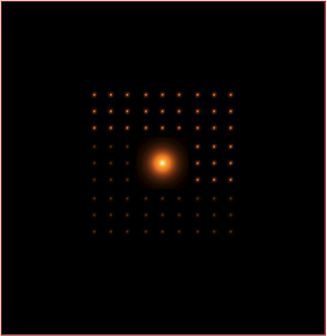
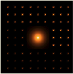
Figure 5.46: Panel a (left): Truth map of Case 5 (fast-scan mode, $\rm 3.5\times 3.5$ deg²); in the PLW band. Panel b (right): Truth map of Case 8 (parallel mode, $\rm 1.4\times 1.4$ deg²); in the PLW band.

5.3.2 Analyses and Results

Point Sources: PSF Fitting

Using PSF fitting method, we checked the following properties of point sources in maps made by different map-makers:

• Astrometry (position offsets);

• flux errors;

• faint source detection rate.

We chose to use the source extractor Starfinder [5] for this task. Starfinder was designed particularly for point sources in crowded field, matching ideally with our test cases which are point sources in confusion limited backgrounds. The detection threshold is set at $\rm 3\sigma$ (local). For a given band in a given case, same PSF (taken from the truth, including pixelization effect) was used for maps made by different map-makers.

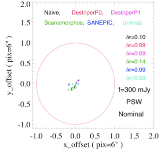
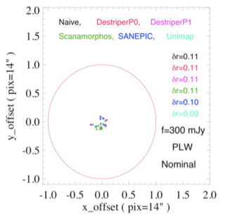
Figure 5.47: Position offsets (relative to the truth, in units of pixel) of bright sources (f=300 mJy) in Case 1 (nominal mode). The left panels are for sources in the PSW band, and right panels for sources in the PLW band. Results on maps made by different map-makers are color coded (as shown in the figures). $\rm\delta r$ is the mean of $\rm\sqrt{x^{2}_{offset}+y^{2}_{offset}})$.

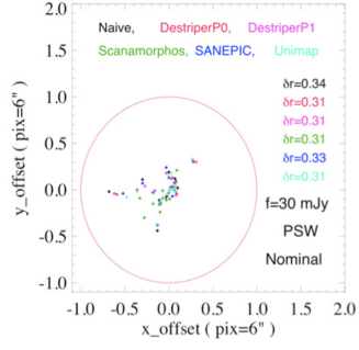
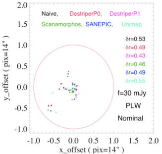
Figure 5.48: Same as Fig. 5.48, for faint sources (f=30mJy).

In Fig. 5.48, the position offsets of the bright sources (f=300 mJy) in Case 1 (nominal mode) are plotted. In a given map, when searching for a correspondence to a “truth source” (searching radius = 1 pixel), we always pick the one closest to the truth position. If there is no detection within the searching radius, the simulated source is deemed undetected. For the bright sources, the offsets are pretty small in all maps, on the order of 0.1 pixels. The offsets of the bright sources in Scanamorphos maps are somewhat larger than in other maps (e.g., in the PSW band, the former have a mean $\rm\delta r$ of 0.14 pix, while for the same sources in all other maps it is $≤0.10$). There are three possible causes for this. First, Scanamorphos applies a relative gain correction, accounting for the variation of the beam area of different detectors, to the level-1 data. However, because this effect was not included in the simulation, other map-makers did not include correction. Potentially, this correction could change the shape of the PSF and cause larger point source offsets. In order to test this hypothesis, Helene Roussel (the author of Scanamorphos) made additional Case 1 maps using Scanamorphos, this time without the relative gain correction. However, the tests carried out using these new maps produced essentially the same results, indicating the effect due to the relative gain correction is not the cause of the larger position offset. The second possible cause for the larger position offsets is the different method used by Scanamorphos to distribute the signal sampled in a given sky position to adjacent sky pixels. While in other maps (including the truth) the entire signal is assigned to the closest sky pixel, Scanamorphos distributes it among adjacent pixels according to the distance between the sampling point and the pixel center. This indeed can cause a difference between the PSF in a Scanamorphos map from that in the corresponding truth map, which in turn cause the larger offset. In a private correspondence, Helene Roussel cited a previous test which indicated that this is a minor, insignificant effect. The third possibility, which was hinted by results of the metrics on “Deviation from the truth” (c.f. Section 5.1.4), is due to a slight positional offset introduced by the mapper. Indeed, in all position-offset plots (Fig  – 5.52) we see systematic offsets toward the lower-left direction for sources in Scanamorphos maps, consistant with the trend found in the difference maps (.e.g. Fig. 5.21).

For the faint sources (Fig. 5.48), the position offsets in all maps are significantly larger than those of bright sources. Because the flux level of the faint sources is very close to the confusion limit, their positions from PSF fitting can be significantly affected by the blending with background sources. In addition to the PSW and PLW bands, for Case 1 we also simulated and checked the PMW band. The results for the PMW band agree with those in the PSW and PMW band.

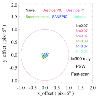
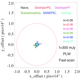
Figure 5.49: Position offsets of bright sources in Case 5 (fast-scan mode).

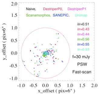
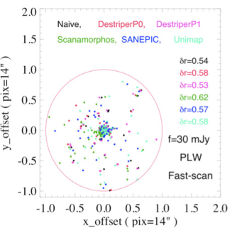
Figure 5.50: Same as Fig. 5.49, for faint sources (f=30mJy).

In Fig. 5.49, the position offsets of the bright sources in Case 5 (fast-scan mode) are plotted. In this case, the map area simulated is much larger than that of the Case 1, and therefore more truth sources were injected (see Section 5.3.1). Here again we see good position accuracy for the bright sources, and slightly larger offsets in the Scanamorphos maps than those in other maps. It is worthwhile noting that these position offsets are somewhat less than those in Case 1 (Fig. 5.48), although the simulated survey in Case 5 is much shallower than that in Case 1 (Table 3.1). Indeed, when comparing the PSW band coverage maps of the Case 5 and of Case 1, we found the coverage of Case 5 is about a factor of 6 shallower than that of Case 1. It appears that the position accuracy of the bright sources is not improved with the depth of the coverage. The reason why the bright sources in nominal observations have poorer position accuracies than those in fast-scan observations, although only marginally significant, needs further investigation. For the faint sources (Fig. 5.50), we see again larger offsets in all maps, and there are no significant differences between results for different map-makers.

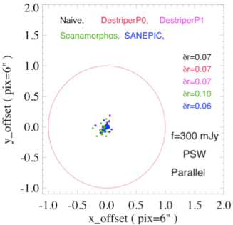
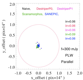
Figure 5.51: Position offsets of bright sources in Case 8 (parallel mode).

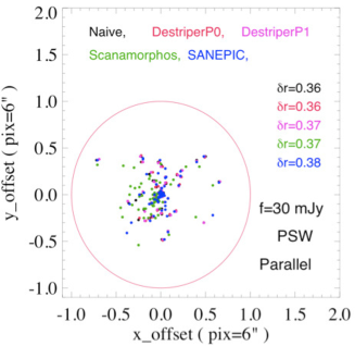
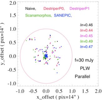
Figure 5.52: Same as Fig. 5.51, for faint sources (f=30mJy).

The position offsets of the point sources in Case 8 (parallel mode) are plotted in Fig. 5.51 and Fig. 5.52. These results are very similar to those for Case 5.

Table 5.6: Position offsets (relative to the truth, in units of pixel), defined as the mean of $\rm\delta r=\sqrt{x^{2}_{offset}+y^{2}_{offset}})$. The bright sources have flux = 300 mJy, and faint sources flux = 30 mJy.

	Case 1				Case 5				Case 8
	PSW		PLW		PSW		PLW		PSW		PLW
	Bright	Faint	Bright	Faint	Bright	Faint	Bright	Faint	Bright	Faint	Bright	Faint
Naive	0.10	0.34	0.11	0.53	0.07	0.51	0.08	0.54	0.07	0.36	0.06	0.46
Destriper-P0	0.09	0.31	0.11	0.49	0.07	0.43	0.08	0.58	0.07	0.36	0.06	0.44
Destriper-P1	0.09	0.31	0.11	0.43	0.07	0.44	0.08	0.53	0.07	0.37	0.06	0.45
Scanamorphos	0.14	0.31	0.11	0.46	0.09	0.56	0.09	0.62	0.10	0.37	0.09	0.49
SANEPIC	0.09	0.33	0.10	0.49	0.07	0.55	0.08	0.57	0.06	0.38	0.06	0.47
Unimap	0.09	0.31	0.09	0.56	0.07	0.53	0.07	0.58

Table 5.7: Dectection rates of bright sources (f = 300 mJy) and faint sources (f = 30 mJy).

	Case 1				Case 5				Case 8
	PSW		PLW		PSW		PLW		PSW		PLW
	Bright	Faint	Bright	Faint	Bright	Faint	Bright	Faint	Bright	Faint	Bright	Faint
Naive	1.0	0.87	1.0	0.25	1.0	0.58	1.0	0.66	1.0	0.88	1.0	0.61
Destriper-P0	1.0	0.87	1.0	0.37	1.0	0.61	1.0	0.69	1.0	0.86	1.0	0.69
Destriper-P1	1.0	0.87	1.0	0.62	1.0	0.55	1.0	0.69	1.0	0.83	1.0	0.69
Scanamorphos	1.0	0.50	1.0	0.50	1.0	0.66	1.0	0.72	1.0	0.88	1.0	0.52
SANEPIC	1.0	0.87	1.0	0.50	1.0	0.63	1.0	0.63	1.0	0.83	1.0	0.66
Unimap	1.0	1.00	1.0	0.37	1.0	0.75	1.0	0.69	1.0

Table 5.8: Fractional flux deviations relative to the truth ($\rm\delta f$) of bright sources (f = 300 mJy) and faint sources (f = 30 mJy).

	Case 1				Case 5				Case 8
	PSW		PLW		PSW		PLW		PSW		PLW
	Bright	Faint	Bright	Faint	Bright	Faint	Bright	Faint	Bright	Faint	Bright	Faint
Naive	0.02	0.08	0.03	0.23	0.02	0.32	0.03	0.29	0.02	0.20	0.03	0.14
Destriper-P0	0.02	0.11	0.02	0.20	0.02	0.28	0.03	0.33	0.02	0.20	0.03	0.16
Destriper-P1	0.02	0.10	0.03	0.19	0.02	0.30	0.03	0.34	0.02	0.18	0.03	0.17
Scanamorphos	0.01	0.17	0.02	0.17	0.02	0.21	0.03	0.24	0.02	0.21	0.02	0.11
SANEPIC	0.02	0.11	0.03	0.14	0.03	0.29	0.04	0.31	0.02	0.22	0.03	0.15
Unimap	0.02	0.12	0.03	0.14	0.03	0.29	0.03	0.24

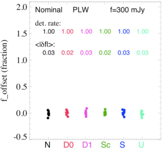
Figure 5.53: Fractional flux deviations (relative to the truth) of bright sources (f = 300 mJy) in Case 1 (nominal mode). Each column is for a given map-maker, color coded in the same way as in Fig. 5.48. The left panels are for sources in the PSW band, and right panels for sources in the PLW band

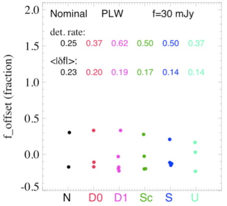
Figure 5.54: Same as Fig. 5.53, for faint sources (f = 30 mJy).

Fraction flux deviations from the truth, as indicators of the flux errors, are plotted in Fig. 5.53 for the bright sources in Case 1 (nominal mode). In each panel, color coded for the different map-makers, the detection rates and the mean flux deviations are also listed. For the bright sources, the detection rates are always 100 percent, and the flux deviations are as low as a couple of percent. There is no significant difference between results for different map-makers. For the faint sources (Fig. 5.54), the detection rate is lower. In particular, in the PLW maps, the detection rates are less or equal to 50%. There are some differences between results for different map-makers. However, combining the results in both PSW and PLW bands, we don’t see any clear pattern. For example, Unimap gives the highest detection rate in the PSW band, but the 2nd lowest detection rate in the PLW band. Then, the detection rate in the PSW map made by Scanamorphos is the lowest among all PSW maps, while in the PLW band, the detection rate in the Scanamorphos map is the 2nd highest. The flux deviations are plotted for the detected faint sources, and the means are listed in the corresponding panels. The deviations are much higher than for those the bright sources, because of the lower signal/noise ratios for the fainter sources.

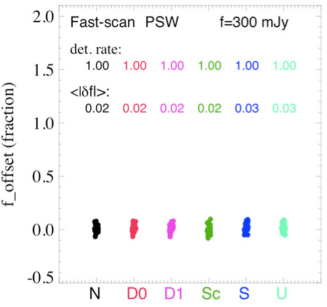
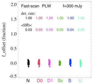
Figure 5.55: Fractional flux deviations of bright sources (f = 300 mJy) in Case 5 (fast-scan mode).

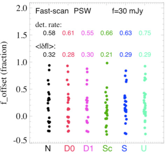
Figure 5.56: Same as Fig. 5.55, for faint sources (f = 30 mJy).

In Fig. 5.55, fractional flux deviations of the bright sources in Case 5 (fast-scan mode) are plotted. The results are very similar to those in Fig. 5.53 (Case 1, nominal mode). However, for the faint sources (Fig. 5.56), there is no significant difference between results in the PSW band and those in the PLW band. Again, there is no significant difference between results for different map-makers.

In Fig. 5.57 and Fig. 5.58, fractional flux deviations of the point sources in Case 8 (parallel mode) are plotted. The results are very similar to those for Case 5 (fast-scan mode).

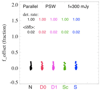
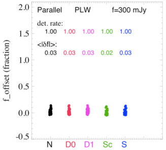
Figure 5.57: Fractional flux deviations of bright sources (f = 300 mJy) in Case 8 (parallel mode).

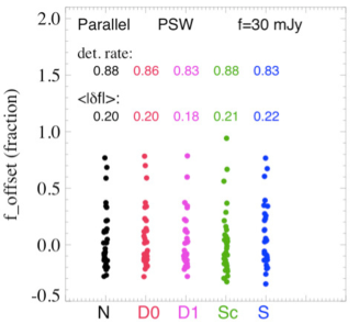
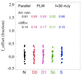
Figure 5.58: Same as Fig. 5.57, for faint sources (f = 30 mJy).

Point Sources: Aperture Photometry

We used two different apertures for the point source aperture photometry. The small aperture has a radius of $\rm 0.5\times FWHM$ of the PSF, and the large aperture a radius of $\rm 2\times FWHM$. The background annulus is between two radii of 3 and 4 times of the FWHM, respectively. The small aperture photometry is sensitive to the position offset, and large aperture photometry checks the energy conservation in the map-making.

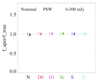
Figure 5.59: Plots of mean $\rm f_{aper}/f_{true}$ ratios of bright sources (f = 300 mJy) in Case 1 (nominal mode); $\rm f_{aper}$ is the flux measured in a simulated map, and $\rm f_{true}$ the flux measured in the corresponding truth map using the same aperture (and background) parameters. In each panel, for a given map-maker, the small point (on the left) with error bars presents the result obtained using the small aperture (r=0.5 FWHM), and the large point (on the right) with error bars the result obtained using the large aperture (r=2 FWHM).

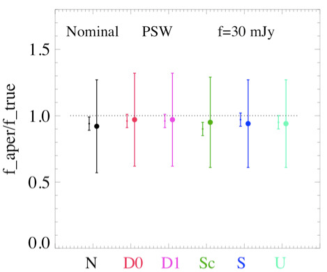
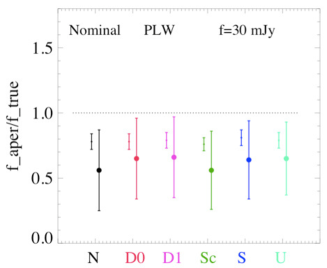
Figure 5.60: Same as Fig. 5.59, for faint sources (f = 30 mJy).

In Fig. 5.59, plots of mean $\rm f_{aper}/f_{true}$ ratios of bright sources in Case 1 (nominal mode) are presented. Here $\rm f_{aper}$ is the flux measured using the aperture photometry in a given map, and $\rm f_{true}$ the flux measured in the corresponding truth map using the same aperture. Using $\rm f_{aper}/f_{true}$ as an indicator for the flux deviation, we are free from uncertainties due to any aperture correction. For the bright sources, both the small and larger aperture photometry agree very well with the truth. There is a slightly under estimation for the large aperture photometry for the naive map in the PLW band. For the faint sources (Fig. 5.60), we see larger deviations and larger error bars because of the noise. In the PLW maps, there is a systematic underestimation of fluxes measured by both apertures, which is apparently due to large confusion noise. Detailed inspections of the maps showed that 5 out of the 8 faint sources are severely affected by blending. The low detection rates shown in Fig. 5.48 are due to the same reason.

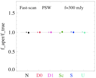
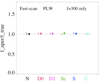
Figure 5.61: Plots of mean $\rm f_{aper}/f_{true}$ ratios of bright sources (f = 300 mJy) in Case 5 (fast-scan mode).

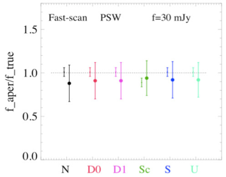
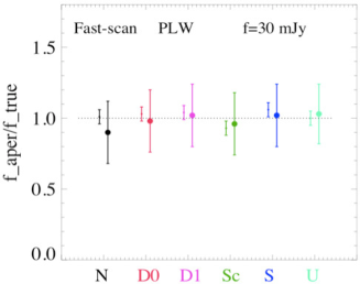
Figure 5.62: Same as Fig. 5.61, for faint sources (f = 30 mJy).

The results for Case 5 (fast-scan mode) are presented in Fig. 17 and Fig. 18. Again we see good photometric accuracy for the bright sources, and large errors for the faint sources. No significant difference is found between results for different map-makers.

Very similar results are found in Fig. 5.63 and Fig. 5.64 for Case 8 (parallel mode).

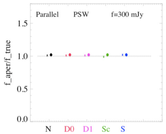
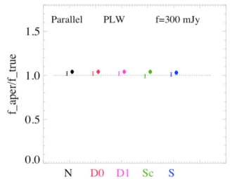
Figure 5.63: Plots of mean $\rm f_{aper}/f_{true}$ ratios of bright sources (f = 300 mJy) in Case 8 (parallel mode).

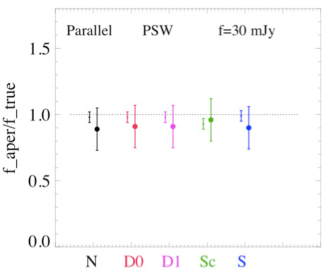
Figure 5.64: Same as Fig. 5.63, for faint sources (f = 30 mJy).

Point Sources: Difference in Beam Profile

In Fig. 5.65, Fig. 5.66 and Fig. 5.67, we compare between the beam profiles of sources in maps made by different map-makers, and the profile of the standard SPIRE PSFs (taken from the SPIRE Photometer beam-profiles release note published on 21 March 2011 by the SPIRE ICC). It appears that, except for the super-resolution map-makers, the beam profiles of sources in maps made by different map-makers do not differ significantly with each other in all cases and in both the PSW and PLW bands. It is interesting to note that, in these figures, the beam profiles of sources in maps made by Scanamorphos look nearly identical as those made by other map-makers. Therefore, although the PSFs in Scanamorphos maps may differ slightly from those in other maps (c.f. Section 4.3), as found in the analysis on the deviation from the truth (Section 5.1), the difference is insignificant on the scale of $\sim 0.2$ pixels (resolution of the beam profile plots in this section).

Also, again in all cases, the beam profiles in the PSW band show a much stronger effect of pixelization than those in the PLW band. A possible explanation for this could be due to a difference between sources in the PSW maps and those in the PLW maps in the simulation: all simulated sources in the PSW maps have their peaks centered at the pixel centers, while for the PLW sources this is true only in Case 1. In Case 5 and Case 8, the source centers in the PLW maps are placed irregularly relative to the pixel centers. So, for the PLW maps in Case 5 and Case 8, we have much better samplings of the PSF phase, therefore much reduced effect of the pixelization. In order to test whether this can indeed be the reason for the pixelization effect, we carried out the following experiment. We made a new Naive PSW map whose orientation is rotated by 45^∘ clockwise relative to the default (north-up) orientation. The rotation of source positions relative to the map grids puts the source centers at different locations relative to the pixel center. In Fig 5.68, we compared the beam profile of the sources in this new map with other results. Indeed the pixelization effects is weakened, in particular for small radii ($\rm<1.5pixel$). However, the pixelization effect remains about the same at larger radii.

The second reason for the PSW beam profiles having stronger pixelization effect could be due to the scan sampling steps, which are  2 arcsec for Case 1 and case 8, and  4 arcsec for Case 5. Given the different sizes of the PLW and PSW beams, these steps may be fine enough for the PSF sampling in the PLW band, but too coarse for that in the PSW band. This may explain the difference between the beem profiles of sources in the PLW map and of those in the PSW map (without rotation) in Case 1, both have centers located at the pixel centers. This may also explain the residual pixelization effect seen in the rotated PSW map in Case 1.

In Fig 5.65 and Fig 5.68, results from HiRes and SUPREME are also included. In the PSW band, the PSF in the HiRes map is indeed much narrower. The PSF in the SUPREME map has about the same FWHM as other map-makers, but has a rather flat center peak. This is perhaps why it has more power in the higher frequency modes in the power-spectra analysis. More detailed analysis on the beam profiles of sources in super-resolution maps can be found in Section 5.4.

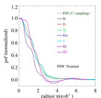
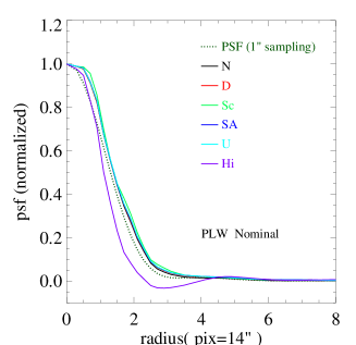
Figure 5.65: Beam profiles for maps in Case 1 (nominal mode), derived using the mean radial distribution of the eight bright sources. The PSF data are taken from the SPIRE Photometer beam-profiles release note published on 21 March 2011 by the SPIRE ICC.

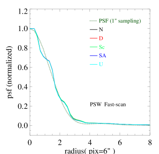
Figure 5.66: Same as Fig. 5.65, for Case 5 (fast-scan mode).

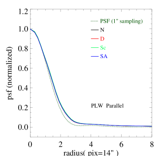
Figure 5.67: Same as Fig. 5.65, for Case 8 (parallel mode).

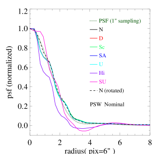
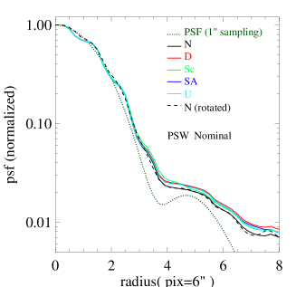
Figure 5.68: Left Panel: Beam profiles for the PSW maps in Case 1. The plot is the same as that in Fig. 5.65, except for an additional beam profile for sources in a map made by NAIVE mapper with crota=45 (the north direction is rotated by 45 degrees clockwise relative to the up direction). Right Panel: The same plot in the logarithmic scale. The beam profiles for sources in the HiRes map and in the SUPREME map are excluded because of the negative values around the minimum. At large radii ($>6$ pix), the noise dominates the signal in the measurements for source profiles in all maps, therefore the values of the measurements are significantly higher than that of the standard PSF.

Extended Source: Aperture Photometry

In all three test cases analyzed here, the central extended source has the same shape of an exponential disk with the e-folding radius of $90”$. The aperture used for its flux measurement has a radius of $\rm r=270”$, namely $\rm 3\times$ e-folding radius. The background annulus is between two radii of 5 and 6 times of the e-folding radius, respectively.

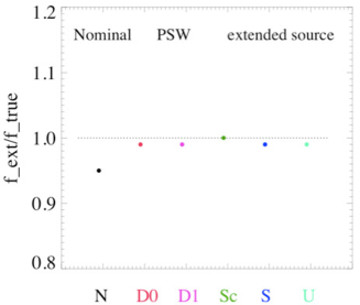
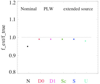
Figure 5.69: Plots of $\rm f_{ext}/f_{true}$ ratios of the extended source in Case 1 maps (nominal mode); $\rm f_{ext}$ is the flux measured in a map made by a given map-maker, and $\rm f_{true}$ the flux measured in the corresponding truth map using the same aperture.

1

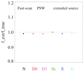
Figure 5.70: Same as Fig. 5.69, for Case 5 (fast-scan mode).

In Fig. 5.69, plots of of $\rm f_{ext}/f_{true}$ ratios of the extended source in Case 1 (nominal mode) are presented. Here $\rm f_{ext}$ is the flux measured in a map made by a given map-maker, and $\rm f_{true}$ the flux measured in the corresponding truth map using the same aperture. We see a significant underestimation in maps made by the naive mapper, in both the PSW and PLW bands. In maps made by other map-makers, the $\rm f_{ext}/f_{true}$ ratio is consistent with unity. For the Case 5 maps in the fast-scan mode (Fig. 5.70), we do not see this difference: the results obtained from the naive maps are as good as those from other maps. The underestimation in the naive maps of Case 1 is due to a known bias in the median baseline removal carried out in the naive map-making, which over-subtracts the background around bright extended sources. The bias is much less significant in Case 5 maps because of the much larger size of the maps (the area occupied by the extended source is much less than the background area). Results for Case 8 maps are similar to those for Case 5 maps.

5.3.3 Summary

1) Both PSF fitting and small aperture photometry show small position errors ($<0.1$ pix) for bright point sources. In some cases, maps made by Scanamorphos show slightly larger errors.

2) Photometry for bright point sources in maps made by all map-makers have small errors, indicating good energy conservation in the map making.

3) The position and the flux errors for the faint sources are significantly affected by the confusion noise. It appears that no map-maker stands out in detecting the faint sources and minimizing the errors.

4) In both PSW and PLW bands, there is no significant difference between beam profiles of sources in maps made by different map-makers. The beam profiles in the PSW band are affected significantly by the pixelization effect.

5) For the photometry of extended sources: in some cases, maps made by Naive mapper are significantly affected by a known bias due to the over-subtraction of baselines. Other maps have no such issue.

5.4 Metrics for Super-resolution Maps (David Shupe)

Since the super-resolution mapmakers for SPIRE are intended for uses different than the other mapmakers, metrics were computed separately for HiRes and SUPREME. The comparisons in this section were made with the Destriped maps (polynomial order=0) as the main reference.

5.4.1 Test Data

A subset of the input data cases were considered for the super-resolution mapmakers.

• Case 1 (sources): simulated data with artificial sources

• Case 10 (cirrus): simulated data with the truth image from a 24 $\mu$m map

• Case 12 (ngc628) : real data of the face-on spiral galaxy NGC 628

• Case 13 (higal_l30): real data of the HiGal $l=30^{\circ}$ field

The maps were made with the standard pixel sizes of [6, 10, 14] arcseconds for [250, 350, 500] $\mu$m. For the sources data (case 1), maps were also made with pixels half the size of the standard ones.

The maps delivered for HiRes were taken from the 20th iteration map and were trimmed to match the area covered by the Destriped map. The delivered SUPREME maps covered a wider area, including all the input data, and had errors in the world coordinates ranging from a few to several dozen pixels. For the analysis reported below, the WCS’s of the SUPREME maps were adjusted based on reference point sources in the images, and the maps were trimmed to cover the same area as the HiRes and Destriped maps. The registration differs by a fraction of a pixel since the projection centers of the SUPREME maps do not fall in the center of a pixel. Since the images are not exactly registered, difference maps are not a useful analysis tool and are not included here.

The analysis focuses on the PSW (250 $\mu$m channel) as SUPREME maps were available for this band only.

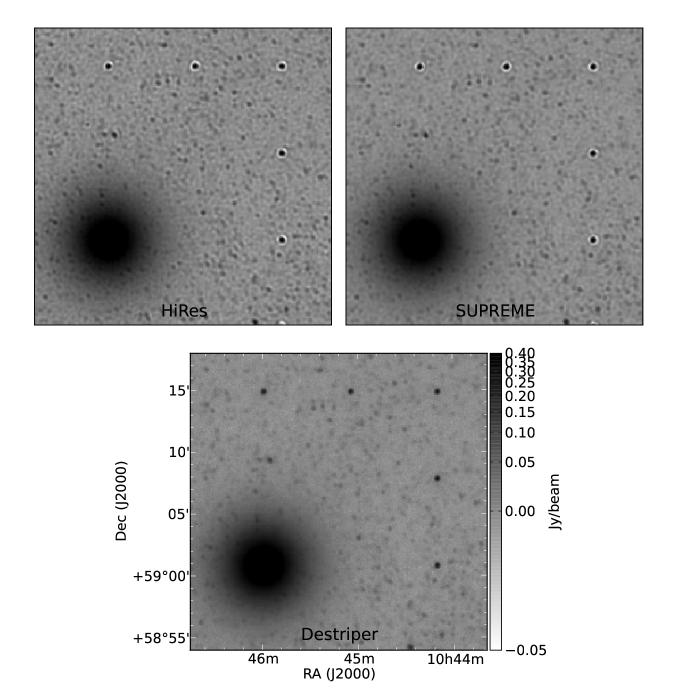
Figure 5.71: Images produced by HiRes, SUPREME, and Destriper, for the 250 $\mu$m band for Case 1 (sources). Part of the field is shown.

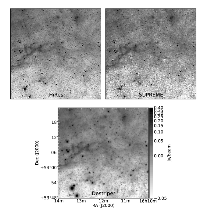
Figure 5.72: Images produced by HiRes, SUPREME, and Destriper, for the 250 $\mu$m band for Case 10 (cirrus), zoomed to part of the field. The ringing around point sources is considered normal, as SUPREME has been designed to enhance the resolution of extended features. The simulation contains many bright point sources because it is based on a 24 $\mu$m map, and is not representative of extended emission observations made with SPIRE.

Figure 5.73: Images produced by HiRes, SUPREME, and Destriper, for the 250 $\mu$m band for Case 12 (NGC 628).

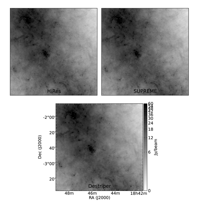
Figure 5.74: Images produced by HiRes, SUPREME, and Destriper, for the 250 $\mu$m band for Case 13 (higal_l30).

5.4.2 Analyses and Results

Power Spectra

Power spectra were computed as an azimuthal average of the 2-D power spectrum. The spectra are normalized to the summed square surface brightness of the maps. The computations were performed with a Python translation of the IDL script provided by Jim Ingalls and described in the preceding chapter on power spectra.

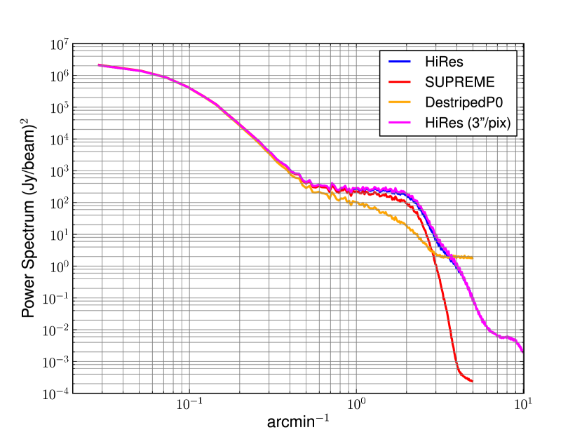
Figure 5.75: Power spectra for the 250 $\mu$m band for Case 1 (sources), including a 3-arcsecond-pixel image for HiRes.

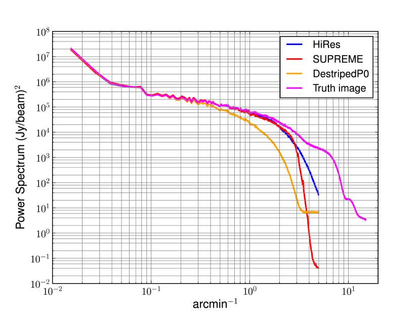
Figure 5.76: Power spectra for the 250 $\mu$m band for Case 10 (cirrus).

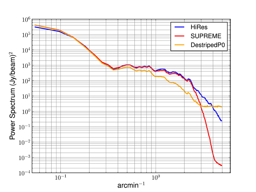
Figure 5.77: Power spectra for the 250 $\mu$m band for Case 12 (NGC 628)

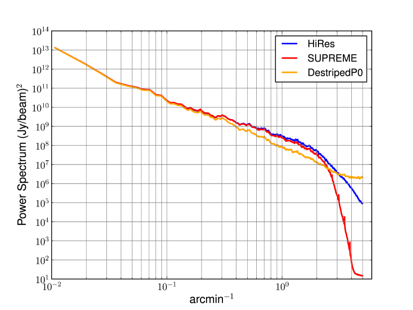
Figure 5.78: Power spectra for the 250 $\mu$m band for Case 13 (higal_l30)

In general, both HiRes and SUPREME perform well, with about a factor of 2-3 improvement in resolution over the destriper at spatial frequencies of about 2 arcmin^-1. The power spectra show that, as designed, SUPREME filters the noise below the beam resolution. HiRes contains more power in the higher frequencies. In more quantitative terms, SUPREME and HiRes power spectra begin diverging at spatial scales between 20 and 24 arcseconds, a size comparable to the FWHM of a Gaussian approximation to the central SPIRE beam at 250 microns. HiRes contains more power than the DestripedP0 map for spatial scales larger than about 15 arcseconds; at smaller scales (higher frequencies) the DestripedP0 map contains more power, visible in the images as noise (not unlike ”snow” seen in old television sets).

Point source profiles

The widths of point sources was estimated by fitting Gaussians to a number of sources in each field. A drawback of this test is that the beams are not Gaussian so the results can be misleading. Therefore these results do not give as complete a picture as the power spectrum analysis provides–the latter analysis is to be preferred in assessing the resolution enhancements provided by these mapmakers.

The results are shown in Table 5.9. The results show improvement in resolution for both map-makers. HiRes FWHM values are reduced by about 25% to 50%, and SUPREME widths are reduced by about 15% to 30%. These figures should be treated with caution, especially since SUPREME is tuned to enhance extended emission, and the SUPREMEX method will provide better separation of point sources.

Case	Map-maker	Number	Mean	Std. Dev
		of sources	FWHM	(FWHM)
			(arcsec)	(arcsec)
1 (sources)	Destriper	10	18.46	1.33
1 (sources)	HiRes	10	13.63	1.22
1 (sources)	HiRes (3 arcsec)	10	13.11	1.15
1 (sources)	SUPREME	10	16.21	0.96
10 (cirrus)	Truthimage	12	6.22	0.20
10 (cirrus)	Destriper	5	22.90	9.1
10 (cirrus)	HiRes	6	11.37	0.42
10 (cirrus)	SUPREME	6	15.43	1.11
12 (NGC 628)	Destriper	12	21.48	0.56
12 (NGC 628)	HiRes	12	13.55	0.74
12 (NGC 628)	SUPREME	12	14.48	0.22

Table 5.9: Results from fitting Gaussians to point sources on the 250 $\mu$m images.

5.4.3 Summary

Overall, both SUPREME and HiRes achieve their goals of resolution enhancement of SPIRE images. For spatial scales larger than about 25 arcseconds in the 250 micron band (comparabale to the beam size), the resolution enhancement of both mapmakers is similar and reaches a maximum of about 2-3 over destriped maps, at spatial frequencies around 2 arcmin^-1. The main difference between SUPREME and HiRes is seen for spatial scales smaller than the beam size. SUPREME is tuned to smooth and reduce the noise at scales smaller than the beam size. The HiRes maps contain more power on these scales, effectively turning noise variations into beam-sized blobs. Fitting Gaussians to point sources shows improvement for both SUPREME and HiRes, with slightly more improvement (25% to 50%) shown by the latter. However it should be noted that SUPREME is tuned to enhance extended emission, and that the power spectrum analysis is to be preferred when assessing gains in resolution.

Chapter 6 Summary

In this report, we present results of a comprehensive test on SPIRE map-making. Seven map-makers participated in this test, including Naive-mapper, Destriper (used in two different configurations), Scanamorphos, SANEPIC, Unimap, HiRes, and SUPREME (the last two being super-resolution mappers). The 13 test cases (8 simulated observations and 5 real observations) include data sets obtained in different observational modes and scan speeds, with different map sizes, source brightness, and levels of complexity of the extended emission. They also include observations suffering from the “cooler burp” effect, and those having strong large-scale gradients in the background radiation. The major goal is to identify strengths and limitations of different map-makers in dealing with different issues in SPIRE maps. The results can be summarized as following:

• The Destriper with the polynomial order of 0 (Destriper-P0), the default map-maker in the SPIRE scanmap pipeline since HIPE 9, performed remarkably well and compared favorably among all map-makers in all test cases except for those suffering from the “cooler burp” effect. In particular, it can handle observations with complex extended emission structures and with large scale background gradient very well.

• In contrast, the Destriper with the polynomial order of 1 (Destriper-P1) compared poorly among its peers, introducing significant artificial large scale gradient in many cases.

• Scanamorphos showed noticeable differences in all comparisons. On the positive side, its maps have the smallest deviation from the truth for faint pixels ($\rm f<0.2Jy$) in nearly all cases. Particularly, as shown in both the difference maps and in the power-spectra, it can handle the “cooler burp” effect very well. On the negative side, for bright pixels ($\rm f>0.2Jy$), its maps show significant deviations from the truth, likely due to a slight positional offset introduced by the mapper as well as a slight change in the beam size. This effect is also seen in the astrometric errors of the bright sources. However the offset is very small ($\sim 0.1$ pexel), therefore it does not affect the photometry of both point sources and extended sources, and does not show up in the comparison between beam profiles (resolution: 0.2 pixels). The power spectrum analysis indicates smoothing of the data compared to the other mapmakers.

• The GLS mapper SANEPIC can also minimize the “cooler burp” effect. It performed quite well in most cases. However, for those cases with strong variations in very large scales (i.e. comparable to the map size), its maps show significant deviations from the truth. This is because some of its assumptions (e.g. TODs are circulant) are invalid for the data.

• Unimap, another participating GLS mapper, is among the best performers in most cases. However, because it does not include a mechanism for handling the “cooler burp”, its maps show significant deviations from the truth in the cases affected by the artifact.

• The Naive-mapper (with simple median background removal) is inferior among its peers in general. The most severe bias it introduces is the over-subtraction of the background when extended emission is present. In the cases where the extended emission is in complex structures, this bias cannot be avoided by simple masks in the background removal.

• The two super-resolution mapmakers, SUPREME and HiRes, yield similar resolution enhancements (factors of 2-3) at spatial scales around 2 arcmin^-1 for the limited datasets tested at 250 microns. At higher spatial frequencies corresponding to spatial scales smaller than the beam size, there is less power in the SUPREME maps (intentionally, to smooth and reduce the noise at scales smaller than the beam). HiRes contains more power than either SUPREME or Destriper-P0 maps between spatial scales of 15-20 arcseconds. The differences in SUPREME and HiRes arise mainly because SUPREME is tuned to enhance extended emission features, and HiRes is essentially performing a deconvolution in image space.

Bibliography

- [1] H.H. Aumann, J.W. Fowler, and M. Melnyk AJ, 1990, 99, 1674.
- [2] H. Ayasso, T. Rodet, and A. Abergel. A GRADIENT-LIKE VARIATIONAL BAYESIAN APPROACH FOR UNSUPERVISED EXTENDED EMISSION MAP-MAKING FROM SPIRE/HERSCHEL DATA. 10 INSU, July 2012.
- [3] H. Ayasso, T. Rodet, and A. Abergel. A variational bayesian approach for unsupervised superresolution using mixture models of point and smooth sources applied to astrophysical map-making. Inverse Problems, 28(12):125005, 2012.
- [4] M. R. Calabretta and E. W. Greisen. Representations of celestial coordinates in FITS. Astronomy and Astrophysics, 395(3):1077–1122, Dec. 2002.
- [5] Diolaiti, E. et al. 2000, SPIE, 4007, 879
- [6] E. W. Greisen and M. R. Calabretta. Representations of world coordinates in FITS. Astronomy and Astrophysics, 395(3):1061–1075, Dec. 2002.
- [7] B. Hasnoun, H. Ayasso, T. Rodet, and A. Abergel. Supreme hipe plugin, January 2013.
- [8] T.H. Jarrett, F. Masci, C.W. Tsai, et. al. AJ, 2012, 144, 68.
- [9] T.H. Jarrett, F. Masci, C.W. Tsai, et al. AJ, 2013, 145, 6.
- [10] F. Masci, astro-ph/1301.2718.
- [11] G. Patanchon, P. A. R. Ade, J. J. Bock, E. L. Chapin, M. J. Devlin, S. Dicker, M. Griffin, J. O. Gundersen, M. Halpern, P. C. Hargrave, D. H. Hughes, J. Klein, G. Marsden, P. G. Martin, P. Mauskopf, C. B. Netterfield, L. Olmi, E. Pascale, M. Rex, D. Scott, C. Semisch, M. D. P. Truch, C. Tucker, G. S. Tucker, M. P. Viero, and D. V. Wiebe. SANEPIC: A Map-Making Method for Timestream Data From Large Arrays. The Astrophysical Journal, 681(1):27, Nov. 2007.
- [12] L. Piazzo, D. Ikhenaode, P. Natoli, M. Pestalozzi , F. Piacentini and A. Traficante: ”Artifact removal for GLS map makers by means of post-processing”, IEEE Trans. on Image Processing, Vol. 21, Issue 8, pp. 3687-3696, 2012.
- [13] L. Piazzo, ’Subspace Least Square Approach for Drift Removal with Application to Herschel Data’, arXiv 1301.1246, 2013.
- [14] Roussel, H. 2012a, arXiv:1205.2576.
- [15] Roussel, H. 2012b, proceedings of the annual meeting of the SF2A, eds. S. Boissier, P. de Laverny, N. Nardetto, R. Samadi, D. Valls-Gabaud and H. Wozniak, pp. 559-563.
- [16] B. Sibthorpe, M. Ferlet, G. Bendo, A. Papageorgiou, and the SPIRE ICC. Spire beam model release note, March 2011. version 1.1.
- [17] M. Tegmark, ”How to make maps from cosmic microwave background data without losing information”, The Astrophysical Journal, 480, pp. L87-L90, May 1997.
- [18] http://w3.uniroma1.it/unimap
- [19] http://herschel.asdc.asi.it/index.php?page=unimap.html