Triplet absorption spectroscopy and electromagnetically induced transparency

Abstract

Coherence phenomena in four-level atomic system, cyclicly driven by three coherent fields, are investigated thoroughly at zero and weak magnetic fields. Each strongly interacting atomic state is converted to a triplet due to a dynamical Stark effect. Two dark lines with a Fano-like profile are arising in the triplet absorption spectrum with anomalous dispersions. We provide the conditions to control the widths of the transparency windows by means of the relative phase of the driving fields and the intensity of the microwave field, that closes the optical system loop. The effect of the Doppler broadening on results of the triplet absorption spectroscopy is analysed in detail.

I Introduction

The absorption spectrum of two-level atomic system exhibits Lorentzian line shape in the absence of any driving field zub . The spectrum is modified when the excited state is coupled to another excited state by a strong laser field. As a result, each excited state splits on two components. This is so-called the Autler-Townes (AT) doublet Autler ; Fano ; Agarwal001 that has been extensively studied in context of spontaneous emission spectrum Agassi ; Zhu-Narducci ; Pasp , stimulated absorption Ph ; Bjor ; Gray ; Delsart ; Fisk , wave mixing Yanp ; Zhiq ; Yig ; Yanp01 , to name just a few. Indeed, the doublets appear in various 3-level atomic or molecular systems interacting with a strong laser field eit . In absorption spectra of such systems a dark line appears in the probe excitation signal under the ideal conditions. That dark line, which is the essence of Electromagnetically Induced Transparency (EIT) eit ; eit02 , is due to a quantum interference between two alternative indistinguishable transition pathways created by the coupling fields with internal states of a quantum system. The EIT is also the manifestation of the Fano-like interference. This interference is characterised by the asymmetric line shape of a resonance spectrum, which is created by various mechanisms in different quantum systems mir . In particular, this asymmetric line shape of resonances has been predicted in atomic ionization due to laser-induced continuum structure (for a review see prk ). The possibility to altering losses of optical beams by strong laser fields attracts researches to employ the EIT based schemes, for example, to slow the group velocity of a subluminal optical probe pulse transmitted by optical media (for a review see nov ) .

The phenomenon of the AT doublet absorption spectroscopy can be further generalized when a multi-level atom is considered. It is expected that the Fano-like interference will be present in this case as well. Evidently, the multiplicative action of these mechanisms in multi-level atom under strong laser fields opens a new avenue to explore various aspects of the absorption cancellation absent in the AT doublet spectroscopy. In fact, a connection of a triplet spectroscopy with the EIT presents a real challenge to the field of atomic spectroscopy Related . Note, that the ability to control, for example, the properties of double EIT (which is absent in the case of 3-level systems): two transparency windows convert to one and vise versa, - may be used as an optical switcher in nanophotonics.

To elucidate typical features of a triplet absorption spectroscopy we consider four-level atomic schemes with different radiative decay mechanisms, cyclicly driven by three coherent fields. In addition, our systems interact with the microwave field which frequency is much smaller of those of the optical fields. It will be shown that the variation of the intensities and phases of optical and microwave fields enables to one to control the degree of super- and sub-luminality in the transparency windows in the absorption triplet spectroscopy. The influence of the Doppler broadening, important from experimental point of view, will be taken into account in our consideration. In this case the mismatch of the optical and microwave frequencies will be analysed thoroughly.

The structure of the paper is as follows. In Sec. II we introduce our model. The Doppler broadening and the vector mismatch are highlighted here as well. In Sec.III we discuss various aspects of triplet absorption spectroscopy, when there are multiple decay channels. Sec.IV is devoted to the analysis of triplet absorption spectroscopy, when there is only one decay channel. Main conclusions are summarized in Sec.V.

II The Model

II.1 Stationary electrical susceptibility

As a typical example of atomic system, interacting with optical fields, we consider first the atomic scheme similar to the Sodium $Na^{23}$ D1 line (3S${}_{1/2}^{2}\Longleftrightarrow$ 3P${}_{1/2}^{2}$) with $\lambda=5895.93{\textup{\AA}}$ at nonzero spin-orbit interaction and zero magnetic field (see Fig.1). Levels 3²P${}_{1/2},$F=2 ($\left|a\right\rangle$) and 3²P${}_{1/2},$F=1 ($\left|b\right\rangle$) of the excited doublet are driven by a microwave field with the Rabi-frequency $\Omega_{m}$. These closely spaced levels are coupled with the ground state 3 ²S${}_{1/2},$F=2 ($\left|c\right\rangle$) by means of two coherent optical fields with the Rabi frequencies $\Omega_{o_{1}}$ and $\Omega_{o_{2}}$.

Excited states decay to the lowest ground state, 3²S${}_{1/2},$F=2 ($\left|c\right\rangle$) and 3²S${}_{1/2},$F=1 ($\left|d\right\rangle$) by means of allowed electric dipole transitions. A weak probe field (with the Rabi frequency $\Omega_{p}$) couples the lowest ground state $\left|d\right\rangle$ and the excited state $\left|a\right\rangle$. We define the optical field detuning parameters as: $\Delta_{o_{1}}=\omega_{ca}-\omega_{o_{1}}$, $\Delta_{o_{2}}=\omega_{cb}-\omega_{o_{2}}$. The detuning parameters of the microwave and probe fields are $\Delta_{m}=\omega_{ba}-\omega_{m}$, and $\Delta_{p}=\omega_{da}-\omega_{p}$, respectively. Here, the frequencies $\omega_{o_{1},o_{2}}$ are associated with two optical fields, $\omega_{m}$ corresponds to the microwave field, while the frequency $\omega_{p}$ characterises the probe field.

In general, the Rabi frequencies can be complex $\Omega_{i}=|\Omega_{i}|\exp(i\phi_{i})\,,i=o_{1},o_{2},m,p$. For the sake of simplicity, we consider the phase associated with the probe field to be fixed as $\phi_{p}=0$. Below, for the sake of convenience, we omit the modulus, i.e., $|\Omega_{i}|\Rightarrow\Omega_{i}$.

The response of a medium due to interaction of these fields with the atomic system under consideration can be found with the aid of the susceptibility of the system (see for details zub )

$$\chi=\frac{N\wp_{ad}}{\epsilon_{0}E}\rho_{ad}\,.$$ (1)

Here, $\wp_{ad}$ is a dipole matrix element, $N$ is number density of atom gas, and $\rho_{ad}$ is the density matrix element between states $|a\rangle$ and $|d\rangle$.

To trace a dynamical behaviour of the probe pulse in the medium we need to evaluate the group index for our system. It is related to the group velocity $v_{g}$ via $N_{g}$=c/$v_{g}$, where c is the speed of light in a vacuum. The group index is calculated as:

$$N_{g}=1+2\pi\mathrm{Re}[\chi]+2\pi\omega_{ad}\mathrm{Re}[\frac{\partial\chi}{\partial\Delta_{p}}].$$ (2)

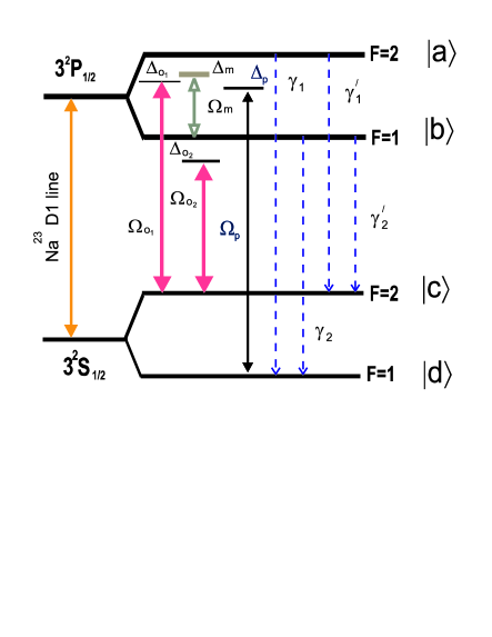
Figure 1: (Color online) A sketch of the atomic energy spectrum of Sodium D1 line at zero magnetic field.

Thus, to analyse the response of our systems to external fields, we have to know the time evolution of the density matrix $\rho_{ad}$. To solve that problem we employ the master equation in Lindblad form

$$\frac{d\rho}{dt}=-\frac{i}{\hbar}[H_{I},\rho]+\Lambda\rho\,,$$ (3)

with a damping term:

$$\Lambda\rho=-\frac{1}{2}\Gamma\sum(\sigma^{\dagger}\sigma\rho+\rho\sigma^{\dagger}\sigma-2\sigma\rho\sigma^{\dagger}).$$ (4)

Here $\sigma=\left|a\right\rangle\left\langle d\right|$ or $\left|b\right\rangle\left\langle d\right|$ and $\sigma^{\dagger}=\left|d\right\rangle\left\langle a\right|$ or $\left|d\right\rangle\left\langle b\right|$ are the lowering and raising operators for the two decay transitions of the system, respectively. In particular, for the spontaneous decay rate of the excited state $3^{2}P_{3/2}\rightarrow 3^{2}S_{1/2}$ one has

$$\Gamma=\frac{1}{4\pi\varepsilon_{0}}\frac{4|\wp_{ad}|^{2}\omega_{da}^{3}}{3\hbar c^{3}}\equiv\gamma\,.$$ (5)

Our system is described by the Hamiltonian, taken in the interaction representation and in the rotating wave approximation (see for details of derivation, for example, zub ):

$$H_{I} =-\frac{\hbar}{2}[\Omega_{m}e^{i(\Delta_{m}t+\varphi_{m})}\left|a\right\rangle\left\langle b\right|+\Omega_{o_{1}}e^{i(\Delta_{o_{1}}t+\varphi_{o_{1}})}\left|a\right\rangle\left\langle c\right|$$ (6)

$$+\Omega_{o_{2}}e^{i(\Delta_{o_{2}}t+\varphi_{o_{2}})}\left|b\right\rangle\left\langle c\right|+\Omega_{p}e^{i\Delta_{p}t}\left|a\right\rangle\left\langle d\right|]+H.c.$$

To proceed further, we use the transformations

$$\rho_{ad}\rightarrow\tilde{\rho}_{ad}e^{i\Delta_{p}t}\,,$$

$$\rho_{cd}\rightarrow\tilde{\rho}_{cd}e^{-i(\Delta_{o_{1}}-\Delta_{p})t}\,,$$

$$\rho_{bd}\rightarrow\tilde{\rho}_{bd}e^{-i(\Delta_{m}-\Delta_{p})t}\,,$$ (7)

$$\rho_{ba}\rightarrow\tilde{\rho}_{ba}e^{-i\Delta_{m}t}\,,$$

$$\rho_{cd}\rightarrow\tilde{\rho}_{cd}e^{-i\Delta_{o_{1}}t}\,.$$

By means of (3,4), in virtue of the transformation (II.1), one obtains the following three coupled rate equations for slowly varying amplitudes (in the first order of the probe field and all orders of the coherent driving fields)

$$\frac{d\tilde{\rho}_{ad}}{dt} = -[i\Delta_{p}+\frac{1}{2}(\gamma_{1}+\gamma^{\prime}_{1})]\tilde{\rho}_{ad}+\frac{i}{2}\Omega_{m}e^{i\varphi_{m}}\tilde{\rho}_{bd}+$$ (8)

$$+ \frac{i}{2}\Omega_{o_{1}}e^{i\varphi_{o_{1}}}\tilde{\rho}_{cd}-\frac{i}{2}\Omega_{p}(\tilde{\rho}_{aa}-\tilde{\rho}_{dd})\,,$$

$$\frac{d\tilde{\rho}_{bd}}{dt} = -[i(\Delta_{p}-\Delta_{m})+\frac{1}{2}(\gamma_{2}+\gamma^{\prime}_{2})]\tilde{\rho}_{bd}+$$ (9)

$$+ \frac{i}{2}\Omega^{\star}_{m}e^{-i\varphi_{m}}\tilde{\rho}_{ad}+\frac{i}{2}\Omega_{o_{2}}e^{i\varphi_{o_{2}}}\tilde{\rho}_{cd}-\frac{i}{2}\Omega_{p}\tilde{\rho}_{ba}\,,$$

$$\frac{d\tilde{\rho}_{cd}}{dt} = -i(\Delta_{p}-\Delta_{o_{1}})\tilde{\rho}_{cd}+\frac{i}{2}\Omega_{o_{1}}e^{i\varphi_{o_{1}}}\tilde{\rho}_{ad}+$$ (10)

$$+ \frac{i}{2}\Omega_{o_{2}}e^{i\varphi_{o_{2}}}\tilde{\rho}_{bd}-\frac{i}{2}\Omega_{p}\tilde{\rho}_{ca}.$$

It is natural to employ the following initial state conditions: $\tilde{\rho}_{dd}=1$, $\tilde{\rho}_{aa}=0$, $\tilde{\rho}_{ba}=0$, $\tilde{\rho}_{ca}=0$. The above set of equations can be solved for $\tilde{\rho}_{ad}$ with the aid of the equation

$$R(t)=\int_{-\infty}^{t}e^{-Q(t-t^{\prime})}Pdt^{\prime}=Q^{-1}P,$$ (11)

where $R(t)$ and $P$ are column matrices, while Q is a 3x3 matrix.

The solution is:

$$\tilde{\rho}_{ad}=-\mathrm{Re}[\tilde{\rho}_{ad}]-i\mathrm{Im}[\tilde{\rho}_{ad}]$$ (12)

with

$$\mathrm{Re}[\tilde{\rho}_{ad}] = \frac{2(\gamma_{2}+\gamma_{2}^{\prime})B_{G}(\Delta_{o_{1}}-\Delta_{p})+R_{G}A_{G}}{A_{G}^{2}+B_{G}^{2}}\Omega_{p}\,,$$ (13)

$$\mathrm{Im}[\tilde{\rho}_{ad}] = \frac{2(\gamma_{2}+\gamma_{2}^{\prime})A_{G}(\Delta_{o_{1}}-\Delta_{p})-R_{G}B_{G}}{A_{G}^{2}+B_{G}^{2}}\Omega_{p}\,.$$ (14)

Here, we use the following notations:

$$A_{G} =-2(\Delta_{m}-\Delta_{p})[(\gamma_{1}+\gamma_{1}^{\prime})(\gamma_{2}+\gamma_{2}^{\prime})$$

$$+4\Delta_{o_{1}}\Delta_{p}-4\Delta_{p}^{2}+\Omega_{m}^{2}]-2\Delta_{o_{1}}\Omega_{o_{1}}^{2}$$

$$+2\Delta_{p}(\Omega_{o_{1}}^{2}+\Omega_{o_{2}}^{2})+2\Omega_{o_{1}}\Omega_{o_{2}}\Omega_{m}\cos\varphi,\,$$

$$B_{G} =(\gamma_{1}+\gamma_{1}^{\prime})[4(\Delta_{p}-\Delta_{m})(\Delta_{o_{1}}-\Delta_{p})+\Omega_{o_{2}}^{2}]$$ (16)

$$+(\gamma_{2}+\gamma_{2}^{\prime})[4(\Delta_{m}-\Delta_{p})\Delta_{p}+\Omega_{o_{1}}^{2}]\,,$$

$$R_{G} =4(\Delta_{o_{1}}-\Delta_{p})(\Delta_{p}-\Delta_{m})+\Omega_{o_{2}}^{2}\,,$$ (17)

and introduce a relative phase $\varphi=\varphi_{o_{1}}+\varphi_{o_{2}}-\varphi_{m}$.

Thus, we have derived general expressions for the real and imaginary parts of the density matrix $\tilde{\rho}_{ad}$, that allow us to analyse optical properties of an ideal four-level atomic scheme displayed on Fig.1.

II.2 The Doppler broadening

To model an experimental situation we have to take into account the random motion of atoms due to thermal energy. Thermal atomic motion produces a spreading of the absorbed frequency. It results in the broadening of the optical profiles, so-called the Doppler broadening. As a result, for each field ”i” the detuning $\Delta_{i}$ should be replaced by $\Delta_{i}+k_{i}v$, where $k_{i}=\omega_{i}/c$ the wavevector of that field. We assume, however, that optical fields have similar transition frequencies

$$k\approx k_{o_{1}}\approx k_{o_{2}}\approx k_{p}\,.$$ (18)

Below we consider a case, when the optical, the microwave and the probe fields propagate collinearly along the $+z$ direction. The microwave frequency is much smaller then those of other driving fields. Therefore, the wave vector of the microwave field can be synchronized with the wave vectors of the optical fields through the two-photon resonance condition as

$$\Delta_{m}\approx[(\Delta_{o_{1}}-\Delta_{o_{2}})+\beta kv],$$ (19)

where $\beta\approx k_{m}/k$.

Taking into account the above conditions that lead to the velocity dependent terms: $\Delta_{m}\rightarrow(\Delta_{m}+\beta kv)$, $\Delta_{o_{1}}\rightarrow(\Delta_{o_{1}}+kv)$, $\Delta_{o_{2}}\rightarrow(\Delta_{o_{2}}+kv)$ and $\Delta_{p}\rightarrow(\Delta_{p}+kv)$, we obtain the following form for the susceptibility

$$\chi(kv)=\frac{N|\wp_{ad}|^{2}}{\epsilon_{0}\hbar\Omega_{p}}[M(kv)\Omega_{p}]\,,$$ (20)

where

$$M(kv)=-\frac{M_{1}(kv)+M_{2}(kv)+M_{3}(kv)}{A_{G_{D}}^{2}(kv)+B_{G_{D}}^{2}(kv)}\,,$$ (21)

$$M_{1}(kv)=R_{G_{D}}(kv)A_{G_{D}}(kv)\,,$$

$$M_{2}(kv)=2(\gamma_{2}+\gamma_{2}^{\prime})G_{G_{D}}(kv)B_{G_{D}}(kv)\,,$$

$$M_{2}(kv)=iQ(kv)\,.$$

Here,

$$Q(kv)=2A_{G_{D}}(kv)G(kv)[(\gamma_{2}+\gamma_{2}^{\prime})-(\Delta_{p}+kv)]$$

$$-R_{G_{D}}(kv)B_{G_{D}}(kv)\,,$$ (22)

$$G_{G_{D}}(kv)=[\Delta_{o_{1}}-\Delta_{p}]\,,$$ (23)

and we have obtained the following expressions

$$A_{G_{D}} =-2[(\Delta_{m}+\beta kv)-(\Delta_{p}+kv)]\times[(\gamma_{1}+\gamma_{1}^{\prime})(\gamma_{2}+\gamma_{2}^{\prime})$$ (24)

$$+4(\Delta_{o_{1}}+kv)(\Delta_{p}+kv)-4(\Delta_{p}+kv)^{2}+\Omega_{m}^{2}]$$

$$-2(\Delta_{o_{1}}+kv)\Omega_{o_{1}}^{2}+2(\Delta_{p}+kv)(\Omega_{o_{1}}^{2}+\Omega_{o_{2}}^{2})$$

$$+2\Omega_{o_{1}}\Omega_{o_{2}}\Omega_{m}\cos\varphi\,,$$

$$B_{G_{D}} =4[(\Delta_{p}+kv)-(\Delta_{m}+\beta kv)]$$ (25)

$$\times[(\gamma_{1}+\gamma_{1}^{\prime})(\Delta_{o_{1}}-\Delta_{p})+(\gamma_{2}+\gamma_{2}^{\prime})(\Delta_{p}+kv)]$$

$$+(\gamma_{1}+\gamma_{1}^{\prime})\Omega_{o_{2}}^{2}+(\gamma_{2}+\gamma_{2}^{\prime})\Omega_{o_{1}}^{2}\,,$$

$$R_{G_{D}} =4(\Delta_{o_{1}}-\Delta_{p})[(\Delta_{p}+kv)-(\Delta_{m}+\beta kv)]+\Omega_{2}^{2}.$$ (26)

Thus, we obtain for the average susceptibility

$$\chi^{(d)}=\frac{N|\wp_{ad}|^{2}}{\epsilon_{0}\hbar V_{D}\sqrt{\pi}}\int_{-\infty}^{\infty}M(kv)e^{-\frac{(kv)^{2}}{V_{D}^{2}}}d(kv)\,,$$ (27)

which is defined with the aid of the Maxwell-Boltzman distribution, where $V_{D}=\sqrt{k_{B}T\omega^{2}/Mc^{2}}$ is the Doppler width. The Doppler width is a free parameter in our numerical examples. The corresponding group index $N_{g}^{(d)}$ has the form (2), where $\chi$ is replaced by $\chi^{(d)}$. Although we present a general scheme, below a thorough analysis is provided for a resonant interaction as an example, i.e., $\Delta_{i}=0,i=o_{1},o_{2},m$.

III Triplet absorption spectroscopy

To proceed further we separate the susceptibility $\chi$ on the imaginary $\Im m\chi\equiv\chi_{\Im}$ and real $\Re e\chi\equiv\chi_{\Re}$ parts

$$\chi_{\Re} = -\frac{N|\wp_{ad}|^{2}}{\epsilon_{0}\hbar\Omega_{p}}\mathrm{Re}[\tilde{\rho}_{ad}]\,,$$ (28)

$$\chi_{\Im} = -\frac{N|\wp_{ad}|^{2}}{\epsilon_{0}\hbar\Omega_{p}}\mathrm{Im}[\tilde{\rho}_{ad}]\,.$$ (29)

It is convenient to measure the absorption and dispersion in the units of $\frac{N|\wp_{ad}|^{2}}{\epsilon_{0}\hbar\Omega_{p}}$. Most BEC experiments reach quantum degeneracy between 500 nK and 2 $\mu$K, at densities between $10^{14}$ and $10^{15}$ cm^-3 ket . For the number density $N\approx 1.3\times 10^{14}$ cm^-3, $\wp_{ad}=2.492\times ea_{0}$ in case of the Sodium D1 line ($a_{0}$ is the Bohr radius) the pre-factor $\frac{N|\wp_{ad}|^{2}}{\epsilon_{0}\hbar}$ is about $2\pi\times 9.89$ MHz. This value could be associated with the spontaneous decay rate $\Gamma$ of the Sodium D1 line.

In the analysis below we use $\Gamma\equiv\gamma_{1}=\gamma$ as a natural unit of the relevant physical quantities and consider Rabi frequency of the weak probe field as $\Omega_{p}=0.1\gamma$ when $\wp_{ad}=2.492\times ea_{0}$ is chosen for the atomic Sodium D1 line. Below some representative examples for the Doppler-free and the Doppler-broadened system are discussed in detail. In this section we consider the value $\varphi=\pi/2$ for the relative phase of the driving fields.

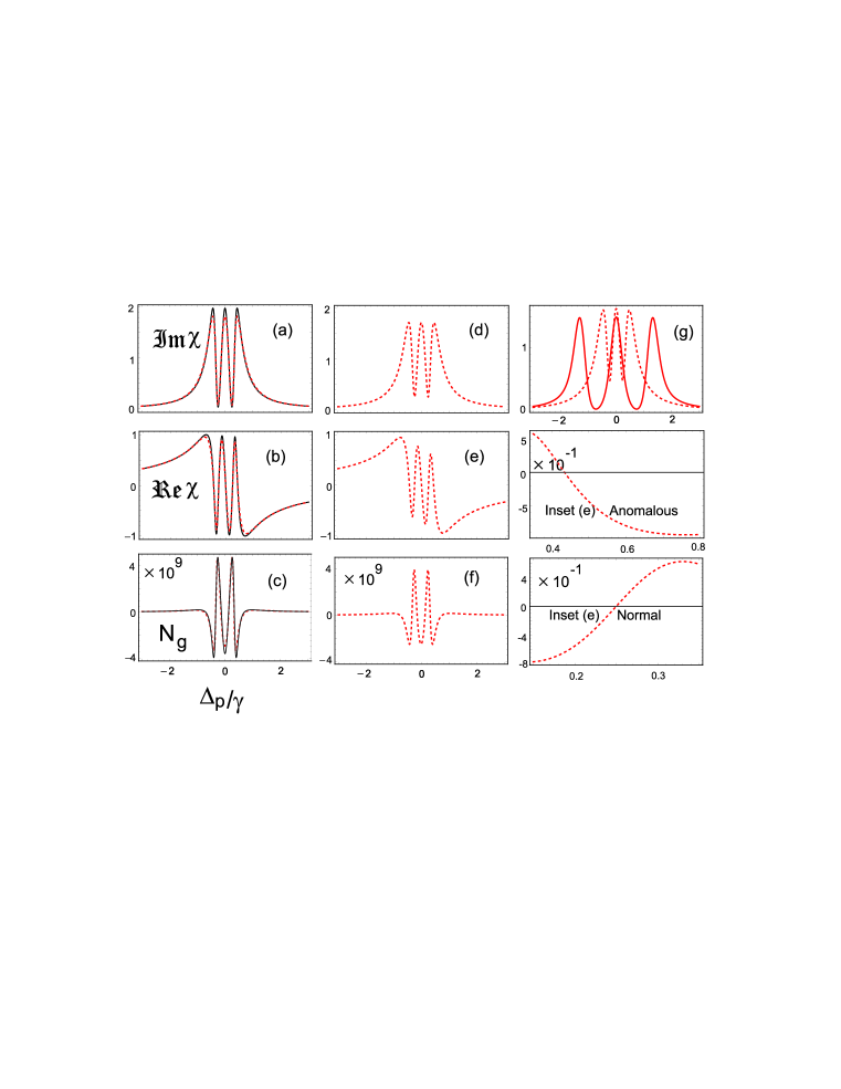
Figure 2: (Color online) Absorption, dispersion, and group index, vs dimensionless probe field detuning $\Delta_{p}/\gamma$. The results at equal intensities $\Omega_{o_{1}}=\Omega_{o_{2}}=\Omega_{m}=0.5\gamma$ (without and with the Doppler broadening, see panels (a), (b), (c)) are connected by solid (black) and dotted (red) lines, respectively. The results at the same intensities (with the Doppler broadening and the vector mismatch $\beta=0.5$, see panels (d),(e), (f)) are connected by dotted (red) line. The results at the vector mismatch $\beta=0.5$ and at equal intensities values: $0.5\gamma$ and $1.5\gamma$ are connected by dotted (red) and solid (red) lines, respectively (see panel (g)). On two right bottom panels the insets for the case (e) are displayed. The following parameters are used: $\omega=10^{8}\gamma$, $V_{D}=0.2\gamma$, $\varphi=\pi/2$, $\gamma_{1}^{\prime}=\gamma_{2}=\gamma_{2}\prime=0.01\gamma$,

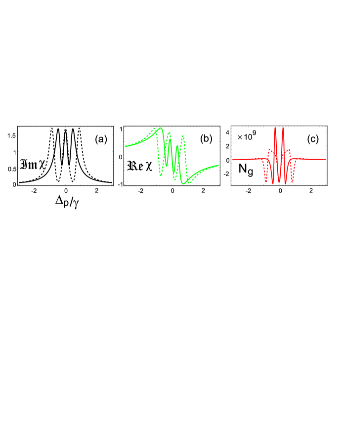
Figure 3: (Color online) Absorption (a), dispersion (b), and group index (c) vs dimensionless probe field detuning $\Delta_{p}/\gamma$ at $\beta=0.5$. The results for $\Omega_{o_{1}}=\Omega_{o_{2}}=\Omega_{m}=0.5\gamma$, and $=\gamma$ are connected by solid and dash lines, respectively. The other parameters are kept the same as in Fig. 2.

III.1 $\Omega_{o_{1}}=\Omega_{o_{2}}=\Omega_{m}\approx\gamma_{1}\gg\gamma_{2},\gamma_{1,2}^{\prime}$

To begin with, we analyze the case, that has been studied by many authors in systems with an excited doublet. For example, Knight and co-workers Pasp analyzed a well known scheme of a quantum beat laser in context of a spontaneous emission, using the same limit.

Generally, when the intensities of all driving fields are kept comparable to the decay rates $\gamma_{1,2}$, the absorption spectrum splits into a triplet tapali ; scully-knight . Note that the triplet is associated with a phenomenon of dynamical Stark triplet splitting. Traditionally it is known as the Autler-Townes splitting.

The positions of the dark lines are determined from the requirement that the numerator of (14) is equal zero. As a result, one obtains the following estimation

$$\Delta_{p}\approx\pm\frac{1}{2}\sqrt{\Omega_{o_{2}}^{2}+\gamma_{2}^{2}}\,.$$ (30)

These dark lines are due to the quantum interference among three alternative indistinguishable transition pathways to the excited state $|a\rangle$. Qualitatively, this result can be understood from the analysis of dressed states of three bare pathways: $|d\rangle\rightarrow|a\rangle$, $|d\rangle\rightarrow|a\rangle\rightarrow|b\rangle\rightarrow|a\rangle$, $|d\rangle\rightarrow|a\rangle\rightarrow|c\rangle\rightarrow|a\rangle$, coupled by two strong optical fields, and the microwave field. However, this analysis requires a separate study and is beyond the scope of the present paper.

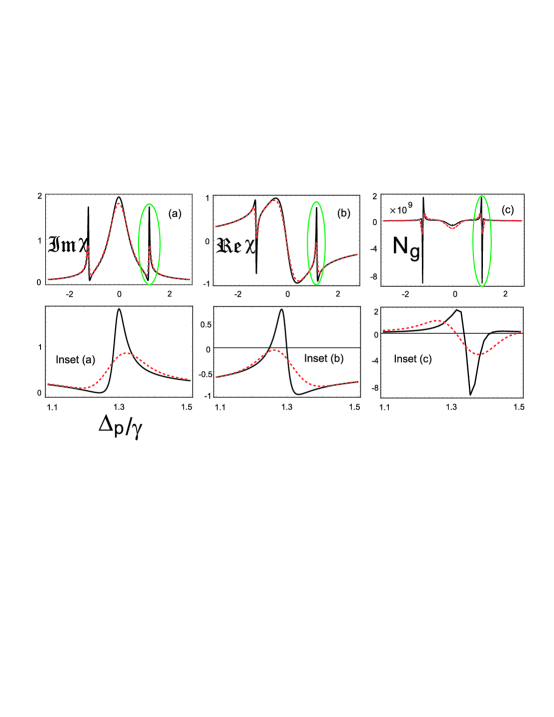
Figure 4: (Color online) Top row: absorption (a), dispersion (b), and group index (c) vs dimensionless probe field detuning $\Delta_{p}/\gamma$. Bottom row: the insets for the case (a)-(c) are displayed. The following parameters are chosen: $\Omega_{o_{1}}=\Omega_{m}=0.5\gamma$ and $\Omega_{o_{2}}=2.5\gamma$. The results at $\beta=0,0.5$ are connected with solid (black) and dashed (red) lines, respectively. The other parameters are kept the same as in Fig.2.

The absorption resonance positions are defined from the requirement $A_{G}=0$ (see (II.1)) that yields three roots. Two of them

$$\Delta_{p}\approx\pm\frac{1}{2}\sqrt{(\Omega_{o_{1}}^{2}+\Omega_{o_{2}}^{2}+\Omega_{m}^{2})+\gamma_{1}(\gamma_{2}+\gamma_{2}^{\prime})}$$ (31)

determine the positions of two side peaks, while the central peak is located at $\Delta_{p}=0$.

Subsequently, it is easy to estimate each peak height, using the corresponding root. The peak width is evaluated as a half of the absorption maximum

$$\frac{\chi_{\Im}}{2}=-\frac{N|\wp_{ad}|^{2}}{B_{G}^{2}\epsilon_{0}\hbar}[(\gamma_{2}+\gamma_{2}^{\prime})A_{G}(\Delta_{o_{1}}-\Delta_{p})-R_{G}B_{G})]\,.$$ (32)

at the corresponding root for $\Delta_{p}$ ($\Delta_{p}=0$, and see (31)).

The quantum interference generates two dark lines that split the absorption spectra into triplets (see Figs.2a,d,g). At equal intensities of the optical and microwave fields, the widths of each components approach the value $\gamma/3$. As compared with the traditional $\Lambda$ and $\Xi$ types of systems, here, in addition to the sub-luminal light, the super-luminal light pulse propagates through the three anomalous dispersive windows with some absorption.

Thus, at equal intensities of the driving fields, there is a dominance of the sub-luminal light over the super-luminal one (see Fig.2c). This dominance can be explained in simple terms. In the insets of Fig.2e we zoom the right wing of the dispersion ${\Re e}\chi$. Evidently, it is related to the absorption spectrum via the Kramers-Kronig relation. While the anomalous dispersion decreases exponentially with the increase of the ratio $\Delta_{p}/\gamma$, the normal dispersion grows faster with the increase of this ratio.

The sub-luminality and super-luminality are affected by the vector mismatch. The vector mismatch $\beta k$ degrades the interference; especially, the super-luminality (compare Figs.2c,f). The increase of the intensity increases the EIT windows (see Fig.2g). However, this increase yields: i)the decrease of the steepness of the transparency windows; and ii) the widening of the absorption spectrum. In addition, it leads to the attenuation of the sub-liminality of the system (see Fig.3). Note, however, that the super-luminality is much less affected.

III.2 $\Omega_{o_{2}}>\Omega_{o_{1}}=\Omega_{m},\gamma_{1}\gg\gamma_{2},\gamma_{1,2}^{\prime}$

At the Doppler free case, it is convenient to estimate analytically the locations of: i) two dark lines; ii) three spectral components; and iii) their widths. By means of the same recipe (see Sec.IIIA), we obtain for the dark line positions

$$\Delta_{p}\approx\pm\frac{1}{2}\sqrt{\Omega_{o_{2}}^{2}+\gamma_{2}^{2}}\,.$$ (33)

In this case the locations of side absorption resonances are determined by (31). Similar to the results of Sec.IIIA, the central peak is located at $\Delta_{p}=0$. In the considered conditions, (32) can be still useful to define the absorption resonance widths. Note that these estimations agree with the corresponding results obtained numerically in the presence of the Doppler broadening and the vector mismatch.

The dominance one of the optical fields with respect to other driving fields leads to the broadening of the central peak, while the side resonances widths are decreasing. In this case the quantum interference of three resonances produce a pattern that is a typical for the Fano-like interference phenomenon mir . The Lorentzian shape of the central peak is complemented by two side resonances with the asymmetric shapes (see Fig.4a).

The super-luminal behavior of the pulse around the two side-windows with the anomalous dispersions is significantly enhanced, when the intensity of the optical field $\Omega_{o_{2}}$ relative to other driving fields is kept high (see Fig.4c). On the other hand, the sub-luminality at two side windows with a normal dispersion get worsened. The largeness and smallness in the positive (negative) group index is correlated through steepness and flatness in the normal (anomalous) dispersion (compare Figs.2(e) and 4(b)).

Thus, the vector mismatch of the microwave field with the other driving fields degrades the interference. The larger is the value of the parameter $\beta$, the larger is the degradation. Although the vector mismatch attenuates strongly the super-luminality in the side transparency windows, the attenuation is much weaker in the central transparency window (see Fig.4(a)). At large strength of the optical field $\Omega_{o_{2}}$ the rate of the atomic oscillations between the second ground state and the excited state is fast as compared with the decay rates of the states of excited doublet. Therefore, the quantum interference is more effective due to the decrease in the decay rates. However, the inherited incoherence, produced by the vector mismatch of the microwave field, may require the larger optical field intensity for its suppression.

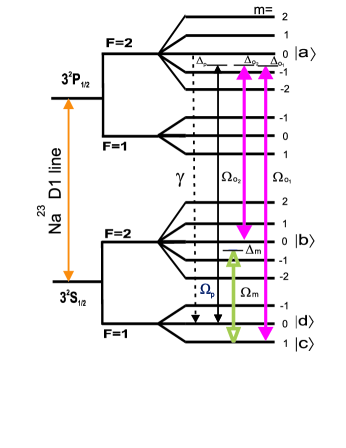
Figure 5: (Color online) A sketch of the atomic energy spectrum of Sodium D1 line at a weak magnetic field.

IV Simplistic triplet absorption spectroscopy

IV.1 One decay channel

The question arises: is it possible to simulate a physical situation, where incoherent processes, discussed above, can be avoided ? Fortunately, this can happen in the scheme based on a simple probability loss, when the contribution of decoherence due to the vector mismatch is relaxed.

Let us consider the Sodium atom in a weak static magnetic field, when there is only one decay channel. Evidently, the Zeeman splitting yields the families of states with different magnetic quantum numbers $m$ (see Fig.5). The microwave field with frequency $\omega_{m}$ couples a low-lying state $|b\rangle$ and a ground state $|c\rangle$ with the Rabi frequency $\Omega_{m}$. These two states are coupled with the excited state $|a\rangle$ by the two optical fields of frequencies $\omega_{o_{1}}$ and $\omega_{o_{2}}$ with the corresponding Rabi frequencies $\Omega_{o_{1}}$ and $\Omega_{o_{2}}$, to form a loop. A weak probe field couples the excited state $|a\rangle$ with a low-lying state $|d\rangle$. The simplicity in the radiative decay process in the present scheme (observed experimentally exp ) provides the proper ground to study the interplay between the driving fields at small decoherence background created by the one decay channel.

This simplistic system is described by the Hamiltonian (taken in the interaction representation and in the rotating wave approximation)

$$H_{I} = -\frac{\hbar}{2}[\Omega_{m}e^{i(\Delta_{m}t+\varphi_{m})}\left|b\right\rangle\left\langle c\right|+\Omega_{o_{1}}e^{i(\Delta_{o_{1}}t+\varphi_{o_{1}})}\left|a\right\rangle\left\langle c\right|$$ (34)

$$+ \Omega_{0_{2}}e^{i(\Delta_{o_{2}}t+\varphi_{o_{2}})}\left|a\right\rangle\left\langle b\right|+\Omega_{p}e^{i\Delta_{p}t}\left|a\right\rangle\left\langle d\right|]+H.c.$$

Applying our approach (see Sec.II) to the Hamiltonian (34), we obtain for the real and imaginary parts of the susceptibility

$$\chi_{\Re}=-\frac{N|\wp_{ad}|^{2}}{\epsilon_{0}\hbar\Omega_{p}}[\frac{R_{S}A_{S}}{A_{S}^{2}+B_{S}^{2}}\Omega_{p}]\,,$$ (35)

and

$$\chi_{\Im}=+\frac{N|\wp_{ad}|^{2}}{\epsilon_{0}\hbar\Omega_{p}}[\frac{R_{S}B_{S}}{A_{S}^{2}+B_{S}^{2}}\Omega_{p}]\,.$$ (36)

Here

$$A_{S} =2(\Delta_{o_{2}}-\Delta_{p})[4\Delta_{p}(\Delta_{p}-\Delta_{o_{1}})-\Omega_{o_{2}}^{2}]-2\Delta_{o_{1}}\Omega_{o_{1}}^{2}$$ (37)

$$+2\Delta_{p}(\Omega_{o_{1}}^{2}+\Omega_{m}^{2})+2\Omega_{o_{1}}\Omega_{o_{2}}\Omega_{m}\cos\varphi\,,$$

$$B_{S} =4\gamma(\Delta_{p}-\Delta_{o_{2}})(\Delta_{o_{1}}-\Delta_{p})+\gamma\Omega_{m}^{2}\,,$$

$$R_{S} =4(\Delta_{o_{1}}-\Delta_{p})(\Delta_{p}-\Delta_{o_{2}})+\Omega_{m}^{2}\,,$$

where $\varphi=\varphi_{m}+\varphi_{o_{1}}-\varphi_{o_{2}}$

Note, that for the Doppler-free system, at the resonance condition $\Delta_{o_{1}}=\Delta_{o_{2}}=0$, the absorption is cancelled if the equation

$$\Delta_{p}=\pm\frac{1}{2}\Omega_{m}$$ (38)

is fulfilled, since $B_{S}=0$. Two dark lines are developed in the Lorentzian type absorption spectrum irrespective of the decay rate and the intensities of the optical fields. However, it is controlled by the intensity of the microwave field. The positions of the central absorption and the sides absorption peaks (components) of the triplet are located at the roots $\Delta_{p}=0$ and

$$\Delta_{p}=\pm\frac{1}{2}\sqrt{\Omega_{o_{1}}^{2}+\Omega_{o_{2}}^{2}+\Omega_{m}^{2}}\,,$$ (39)

respectively, when $A_{S}=0$ at $\varphi=\pi/2$. The widths of each spectral component can be easily evaluated by means of the equation

$$\chi_{\Im}/2=-\frac{N|\wp_{ad}|^{2}}{\epsilon_{0}\hbar B_{S}}\,,$$ (40)

when $\Delta_{p}$ in the expression for $B_{S}$ (see (37)) is replaced either by zero or by the corresponding root of (39).

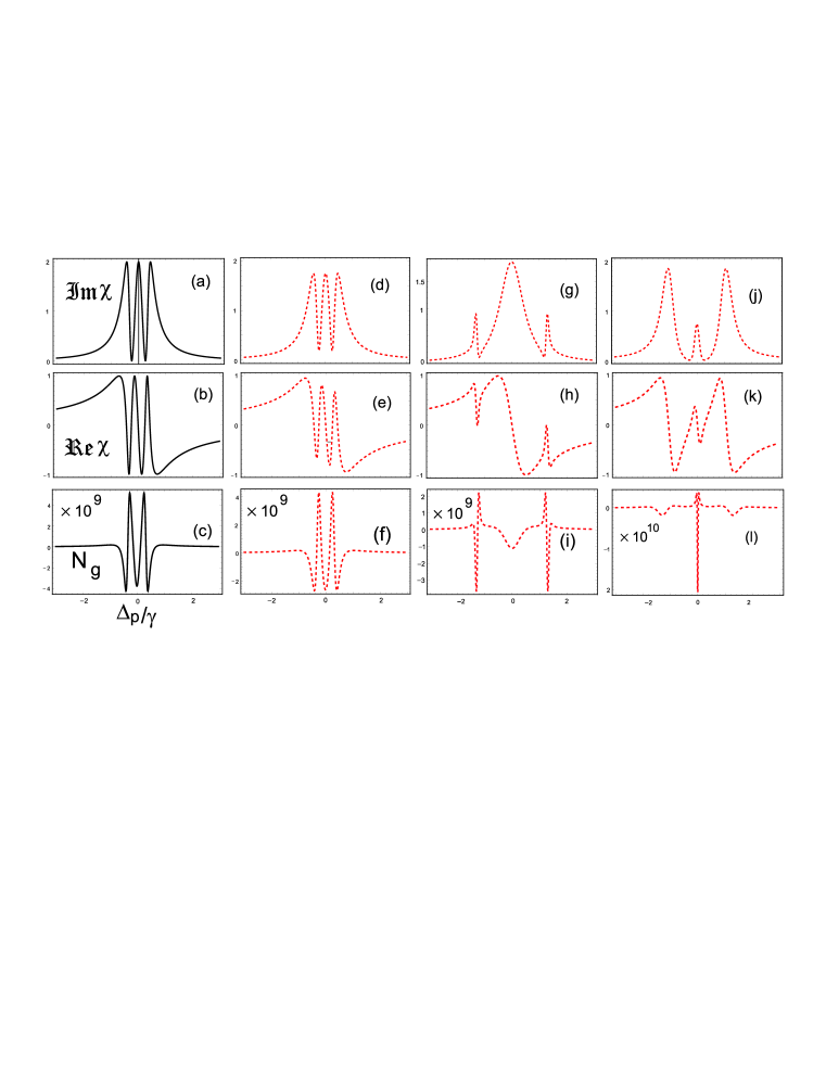
Figure 6: (Color online) Absorption (a,d,g,j), dispersion (b,e,h,k), and group index (c,f,i,l), vs the field detuning, $\Delta_{p}/\gamma$. The following parameters are used: $\omega=10^{8}\gamma$, $V_{D}=0.2\gamma$, $\varphi=\pi/2$. The results for equal intensities $\Omega_{o_{1}}=\Omega_{o_{2}}=\Omega_{m}=0.5\gamma$ are connected by solid (black) line for $\beta=0$ (a-c), and dashed (red) line for $\beta=0.5$ (d-f). The results for $\Omega_{m}=2.5\gamma$, $\Omega_{o_{1}}=\Omega_{o_{2}}=0.5\gamma$, and $\beta=0.5$ are connected by dashed (red) line (g-i). The results for $\Omega_{o_{2}}=\Omega_{m}=0.5\gamma$, $\Omega_{o_{1}}=2.5\gamma$ are connected by dashed (red) line for $\beta=0.5$ (j-l).

Thus, we have derived the system of equations that define the real and imaginary terms of the susceptibility in an ideal case of the one decay channel. As before, a thorough analysis is provided for a resonant interaction as an example, i.e., $\Delta_{i}=0,i=o_{1},o_{2},m$.

IV.2 Doppler broadening and vector mismatch

To trace the influence of the Doppler broadening, we consider the collinear propagation of the microwave field, two optical and the probe fields. This consideration yields the replacements of $\Delta_{m}\rightarrow(\Delta_{m}+\beta kv)$, $\Delta_{o_{1}}\rightarrow(\Delta_{o_{1}}+kv)$, $\Delta_{o_{2}}\rightarrow(\Delta_{o_{2}}+kv)$ and $\Delta_{p}\rightarrow(\Delta_{p}+kv)$ in (35), (36). The synchronization of the microwave field with the optical driving fields requires the condition $\Delta_{o_{2}}=(\Delta_{o_{1}}-\Delta_{m})$ to be fulfilled (the two photon Raman resonance condition).

Taking into account the vector mismatsh $\Delta_{m}\rightarrow(\Delta_{m}+\beta kv)$, we use the substitution $\Delta_{o_{2}}\rightarrow[(\Delta_{o_{1}}-\Delta_{m})+(1-\beta)kv]$ in (35)-(37), in addition to the substitution of the other velocity dependent terms. The average susceptibility is defined as before

$$\chi(kv)=\frac{N|\wp_{ad}|^{2}}{\epsilon_{0}\hbar\Omega_{p}}[\frac{R_{S_{D}}(kv)A_{S_{D}}(kv)+iQ_{S_{D}}(kv)}{A_{S_{D}}^{2}(kv)+B_{S_{D}}^{2}(kv)}\Omega_{p}],$$ (41)

where

$$A_{S_{D}}(kv) =-2(\Delta_{o_{1}}+kv)\Omega_{o_{1}}^{2}+2(\Delta_{p}+kv)(\Omega_{o_{1}}^{2}+\Omega_{m}^{2})$$ (42)

$$+2[[(\Delta_{o_{1}}-\Delta_{m})+(1-\beta)kv]-(\Delta_{p}+kv)]$$

$$\times[4(\Delta_{p}+kv)(\Delta_{p}-\Delta_{o_{1}})-\Omega_{o_{2}}^{2}]$$

$$+2\Omega_{o_{1}}\Omega_{o_{2}}\Omega_{m}\cos\varphi,\,$$

$$B_{S_{D}}(kv) =\gamma\Omega_{m}^{2}+4\gamma(\Delta_{o_{1}}-\Delta_{p})$$

$$\times[(\Delta_{p}+kv)-[(\Delta_{o_{1}}-\Delta_{m})+(1-\beta)kv]],$$

$$R_{S_{D}}(kv) =\Omega_{m}^{2}+4(\Delta_{o_{1}}-\Delta_{p})$$

$$\times[(\Delta_{p}+kv)-[(\Delta_{o_{1}}-\Delta_{m})+(1-\beta)kv]]\,,$$

$$Q_{S_{D}}(kv) =-2A_{S_{D}}(kv)B_{S_{D}}(kv)R_{S_{D}}(kv)\,.$$ (45)

In this system the quantum interference is always dominant for both the Doppler-free and Doppler broadened cases due to simple losses. In fact, this a nice manifestation of the Fano-like interference mechanism in the triplet spectroscopy. In the case of the doublet spectroscopy, at the resonance condition, the position of the dark line is always fixed (see e.g. Refs.zub ; eit ). In our model there are two dark lines in the absorption spectra, independently on the strength of the driving fields at the relative phase $\varphi=\pi/2$ (see top row of Fig.6). Their positions can be changed by the intensity of the microwave field (see (38)). In virtue of this fact, one can tune up the whole system by a proper choice of the optical fields.

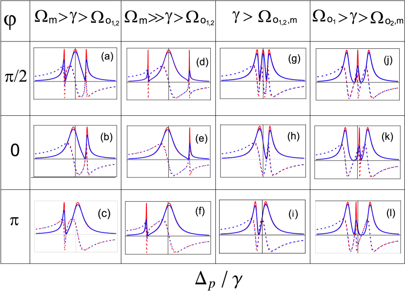
Figure 7: (Color online) Absorption (solid line), dispersion (dashed line) vs dimensionless probe field detuning $\Delta_{p}/\gamma$. The red lines connect the results without Doppler broadening and vector mismatch; the blue lines connect the results with the vector mismatch $\beta k=0.5\gamma$ and the Doppler width $V_{D}=0.2\gamma$. Panels (a,b,c): $\Omega_{o_{1}}=\Omega_{o_{2}}=0.5\gamma,\Omega_{m}=1.5\gamma$. Panels (d,e,f): $\Omega_{o_{1}}=\Omega_{o_{2}=}0.5\gamma,\Omega_{m}=3\gamma$. Panels (g,h,i): $\Omega_{o_{1}}=\Omega_{m}=\Omega_{o_{2}}=0.5\gamma$. Panels (j,k,l): $\Omega_{m}=\Omega_{o_{2}}=0.5\gamma,\Omega_{o_{1}}=1.5\gamma$. The other parameters are kept the same as in Fig.6.

Evidently, the Doppler broadening degrades the system coherence. In addition, the vector mismatch relaxes the sub- and super-liminality (compare Figs.6(a-c) and Figs.6(d-f)) at the equal intensity of the driving fields. However, as it was shown in Sec.IIIB, one can control the properties of the central absorption peak by choosing the appropriate optical field to be dominant over other parameters of the system. In fact, many features are simply the consequence of the Kramers-Kronig relations. Two side and a small central peaks in the absorption spectrum correspond to anomalous dispersions for the probe field. The dominance of the intensity of the optical field $\Omega_{o_{1}}$ yields the drastic increase of the super-luminality (compare Figs.6f,l) and to the attenuation of the sub-luminality of the side peaks.

At the dominance of the microwave field $\Omega_{m}$, for the central broadened peak (see Fig.6g) the dispersion is mild (see Fig.6h). The substantial enhancement in the group index for the steep anomalous regions at the side positions of the absorption spectra is accompanied by the attenuation of the super-luminality at the central position due to the flattened dispersion (compare Figs.6f,i).

Thus, in the proposed scheme one is able to control the transparency windows by means of the external fields in the triplet absorption spectroscopy. The EIT aspect related to the absorption/dispersion properties of the proposed scheme is studied in detail below.

IV.3 Control of the EIT windows

To understand better the quantum interference phenomenon we consider different relative phases $\varphi=0,\pi/2,\pi$ of the driving fields. Note that the results for the phase values $\varphi=0,\pi/2$ represent a mirror reflection of those obtained for the values $\varphi=\pi,3\pi/2$. We summarize our findings in Fig.7, that are also consistent with the results of Sec.III.

Obviously, the spectrum splits into a triplet by two dark lines developed in the Lorentzian type absorption spectrum at $\Delta_{p}=\pm\Omega_{m}/2$ (see Fig.7(g) for $\varphi=\pi/2$). The width of each spectral component appears as $\gamma/3$ when the intensities of the driving fields are kept equal. The quantum interference is always dominant for the Doppler-free and Doppler broadened cases, due to the simple probability loss. The absence of additional radiative decay rates in the system relaxes the influence of the vector mismatch of the microwave field. However, if the microwave field is switched off, the control of the EIT is reduced, since one is faced with the traditional tripod systems (see, e.g., Ref.barry-sender ).

The double transparency windows could exist in the system as well if one of the optical fields is switched off. In this case, the absorption (35) and dispersion (36) spectra become phase insensitive, when either $\Omega_{o_{1}}$ or $\Omega_{o_{1}}$ is set to zero in (42). Therefore, to maintain phase effects in the system, it is important to preserve loop structure couplings of the driving fields.

To illuminate the crucial role of the microwave field and the relative phase of the driving fields, we neglect the effect of the Doppler broadening and focus on the absorption (36) at the resonance condition $\Delta_{o_{2}}=\Delta_{o_{1}}=\Delta_{m}=0$. In this case we have

$$A_{S_{R}} = -8\Delta_{p}^{3}+2\Omega^{2}\Delta_{p}+2\Omega_{o_{1}}\Omega_{o_{2}}\Omega_{m}\cos\varphi,$$ (46)

$$R_{S_{R}} = \Omega_{m}^{2}-4\Delta_{p}^{2}\,,\quad B_{S_{R}}=\gamma R_{S_{R}}\,,$$ (47)

$$\Omega^{2} = \Omega_{o_{1}}^{2}+\Omega_{o_{2}}^{2}+\Omega_{m}^{2}.$$ (48)

We recall that the prefactor ${N|\wp_{ad}|^{2}}/({\epsilon_{0}\hbar})\equiv\gamma$ is our natural unit. Further, for the sake of convenience we introduce the following notations

$$y_{i}=\Omega_{i}/2\gamma\,,\quad i=o_{1},o_{2},m\,,\quad x=\Delta_{p}/\gamma\,.$$ (49)

Taking into account these definitions, it is straightforward to present (36) in the Fano-type form

$$\chi_{\Im}=\frac{(x^{2}-y_{m}^{2})^{2}}{4F^{2}+(x^{2}-y_{m}^{2})^{2}}\,,$$ (50)

$$F=x^{3}-K^{2}x-M\cos\varphi\,,$$ (52)

$$K^{2}=(y_{1}^{2}+y_{2}^{2}+y_{m}^{2})\,,\quad M=2y_{1}y_{2}y_{m}\,.$$

These equations demonstrate clearly the dependence of the absorption on the strength of the microwave field and the relative phase $\varphi$ of the driving fields. It appears that the positions of the dark lines are always determined as $x=\pm y_{m}\Rightarrow\Delta_{p}=\pm\Omega_{p}/2$. However, this result should be taken cautiously, since the phase factor play important role as well.

Evidently, the roots of (52) determine the position of three absorption maxima (see Figs.7a,d,g,j) in general. In particular, at $\varphi=\pi/2$ they are defined by (38,39). There is, however, a significant influence of the relative phase of the driving fields on the tunability of the Fano-like resonances in the triplet absorption spectrum. Two Fano-like resonances can be tuned into a single Fano-like resonance and vise versa in the absorption spectrum if the relative phase of the driving fields is varied.

Indeed, the central absorption peak (see Figs.7a,d,g) merges: either with its left (right) peak at the phase $\varphi=0$ ($\varphi=\pi$) at Figs. 7b,e, (Figs.7c,f), or with its right (left) peak at Fig.7 h (Fig.7i). As an example, we consider the case Fig.7b: $\Omega_{o_{1}}=\Omega_{o_{2}}=0.5\gamma,\Omega_{m}=1.5\gamma,\varphi=0$. By means of (49,50,52,52), one readily obtains

$$\chi_{\Im} = \frac{(x^{2}-9/16)^{2}}{4(x+3/4)^{2}[(x-3/8)^{2}-17/64]^{2}+(x^{2}-9/16)^{2}}$$ (53)

$$= \frac{(x-3/4)^{2}}{4[(x-3/8)^{2}-17/64]^{2}+(x-3/4)^{2}}\,.$$

The position of only one dark line is located at $x=3/4$, while two absorption maxima are determined by $x_{1,2}=3/8\pm\sqrt{17}/8$. In this process, one of the Fano-like resonances (and dark lines) disappears from the spectrum. The width of the merged peak is compensated by the increase of the width of the corresponding side peak. In addition, for a large relative strength, the central broadened peak is merged with the side one (see Figs.7e,f).

Unlike the study in Ref. optomechanics , where the Fano-like resonance was tuned by using some approximation in the opto-mechanics set-up, here the control of the single dynamical variable $\varphi$ is enough to control the resonance profile.

Depending on the phase and relative intensities of the driving fields, the dispersion associated with the central and side components of the absorption spectrum superimposes at the cost of large absorption developed by the merging effect. Subsequently, we are left with one EIT window on either sides of the central line (see Figs.7b,e,h and Figs.7c,f,i). As a result, the height and the width of the absorption peak will increase, and the sub-luminal light is converted to the super-luminal one. We expect that the probe pulse would be greatly attenuated during the propagation through the transparency window with the anomalous dispersion.

Thus, the phase control can be used to convert the double transparency behaviour of the medium to a single transparency one and vise versa. In addition, at dominance one of the optical fields, we obtain a shift of the central peak either to the left ($\phi=0$) or to the right ($\phi=\pi$) side with the respect of its position at ($\phi=\pi/2$) (see Figs.7j,k,l).

Note that the dark line positions with and without the vector mismatch are controlled by the intensity of the microwave field $\Omega_{m}$ (see Figs.7a,d) as well. The larger is the intensity of the microwave field, the widened are the transparency windows, with a similar mirror inversion for the dispersions. The sharper and shorter anomalous dispersions associated with two sides sharp absorption lines are now away from the central location of the spectrum. Therefore, the sub-luminal probe pulse propagation through two windows is degraded. However, once the intensity of the optical field $\Omega_{o_{1}}$, or $\Omega_{o_{2}}$, or both are increased, the normal dispersions get worsen at two windows. Subsequently, the central absorption line becomes extremely narrowed with a giant anomalous dispersion. In response, the slow light through the transparency window becomes degraded extremely (see Figs.7j,k,l).

We conclude that the widths of the three components of the triplet spectrum are not dependent on the frequencies of two optical and microwave fields. We recall that in the traditional one-window based EIT systems the widths of absorption components of the corresponding spectrum are independent on the intensities of control fields. However, in the considered system the widths depend on their intensities and their coupling positions in the interaction loop relative to the decaying energy level. For example, the width of the central component in the considered simplistic scheme is narrowed with the increase of the intensity of the optical field $\omega_{o_{1}}$ or the optical field $\omega_{o_{2}}$, or both of them. On the other hand, the microwave field, coupled indirectly to the decaying energy level, produces the opposite effect. Namely, the width of the central peak is broadened with the increase of the microwave field intensity. In addition, the manipulation of the EIT windows is achieved by means of an effective tuning of the microwave field intensity.

V Summary

We have analysed thoroughly the coherence phenomena produced by three cyclicly driven optical fields in four-level systems at zero and weak magnetic fields. To this aim we have developed the model in order to trace the optical response of the atomic Sodium system, as an example. It was found that in this system the coherence effects yield two dark lines, in general. This is due to the EIT phenomenon which manifests the interplay between the Autler-Townes and the Fano-like mechanisms in a triplet absorption spectroscopy.

To gain a better insight into coherence phenomena we have proposed the ideal but experimentally viable behaviour of our system at the weak magnetic field. We have provided various sets of parameters to explore the transition from a multiple broad-band to extremely narrow-band windows for transparency of the probe pulse. Such effect could exist only when two optical fields are coupled in a combination with a microwave field to form a loop structured interaction. In fact, we found a significant influence of the relative phase of the driving fields on the tunability of the Fano-like resonances in the triplet absorption spectrum. Two Fano-like resonances in the absorption spectrum can be tuned into a single Fano-like resonance and vise versa. We have demonstrated that the degree of the EIT (with and without the Doppler broadening) can be controlled by altering the intensities of the external optical fields as well.

We speculate that the controllability of the EIT windows by means of a manipulation of the intensity of the microwave field and relative phase of the driving fields in the considered system could help to improve some technical aspects of devices already in use or yet to be developed eit . In particular, the coherence and interference phenomena, similar to the EIT in gaseous media and optoelectronic materials eit ; atom-vapor , might promise some logic and functional operations such as NOT and AND gates when a system enables to produce an enhanced double EIT express .

From our calculations it follows that the normal dispersions around the two dark lines are extremely flattened. As a result, the sub-luminality is attenuated (see Fig.6j,k,l). As a matter of fact, it is the microwave field enables to one to control the positions of the dark lines in the triplet spectroscopy, and, subsequently, to change the sub- and super-luminality of the probe pulse.

Steep anomalous dispersions at the corresponding windows are accompanied with a relatively small but sharp absorption. It results in a drastic enhancement of the super-luminal group velocity of the probe pulse. The enhanced group velocity of light promises various experimental applications. For example, the quality of an image measured by a light pulse with a relatively low group velocity could be improved if measured by a super-luminal light pulse with a significantly high group velocity image .

References

- (1) Scully M O and M. S. Zubairy M S 1997 Quantum Optics (Cambridge: Cambridge University Press).
- (2) Autler S H and Townes C H 1955 Phys. Rev. 100 703; Knight P L and Milonni P W 1980 Phys. Rep. 66 23.
- (3) Fano U 1961 Phys. Rev. 124 1866; Fano U and Cooper J W 1968 Rev. Mod. Phys. 40 441.
- (4) Agarwal G S 1991 Phys. Rev. A 44 R28; Wang D and Zheng Y 2011 Phys. Rev. A 83 013810.
- (5) Agassi D 1984 Phys. Rev. A 30 2449.
- (6) Zhu S Y, Narducci L M, and Scully M O 1995 Phys. Rev. A 52 4791.
- (7) Paspalakis E, Keitel C H, and Knight P L 1998 Phys. Rev. A 58 4868.
- (8) Cahuzac P and Vetter R 1976 Phys. Rev. A 14 270.
- (9) Bjorkholm J E and Liao P F 1977 Opt. Commun. 21 132.
- (10) Gray H R and Stroud Jr C R 1978 Opt. Commun. 25 359.
- (11) Delsart C, Keller J C, and Kaftandjian V P 1981 J. Phys. 42 529.
- (12) Fisk P T H, Bachor H A, and Sandeman R J 1986 Phys. Rev. A 33 2418.
- (13) Zhang Y, Anderson B, and Xiao M 2008 J. Phys. B: At. Mol. Opt. Phys. 41 045502.
- (14) Nie Z, Li H Z P, Yang Y, Zhang Y, and Xiao M 2008 Phys. Rev. A 77 063829.
- (15) Du Y et al 2009 Phys. Rev. A 79 063839.
- (16) Zhang Y, Li P, Zheng H, Wang Z, Chen H, Li C, Zhang R, and Xiao M 2011 Opt. Exp. 19 7769.
- (17) Fleishchhauer M, Imamoglu A, and Marangos J P 2005 Rev. Mod. Phys. 77 633.
- (18) Bhattacharyya D, Ray B, and Ghosh P N 2007 J. Phys. B: At. Mol. Opt. Phys. 40 4061; Li S, Yang X, Cao X, Xie C, and Wang H 2007 J. Phys. B: At. Mol. Opt. Phys. 40 3211; Li H, Sautenkov V A, Rostovtsev Y V, Welch G R, Hemmer P R, and Scully M O 2009 Phys. Rev. A 80 023820.
- (19) Miroshnichenko A E, Flach S, and Kivshar Y S 2010 Rev. Mod. Phys. 82 2257.
- (20) Knight P L, Lauder M A, and Dalton B J 1990 Phys. Rep. 190 1.
- (21) Novikova I, Walsworth R L, and Xiao Y 2012 Laser Photonics Rev. 6 333.
- (22) Wang C L, Li A J, Zhou X Y, Kang Z H, Jiang Y, and Gao J Y 2008 Opt. Lett. 33 687; Shen J Q and Zhang P 2007 Opt. Exp. 15 6484.
- (23) Ketterle W 2002 Rev. Mod. Phys. 74 1131.
- (24) Sahrai M, Tajali H, Kapale K T, and Zubairy M S 2006 Phys. Rev. A 73 023813.
- (25) Zhu S Y and Scully M O 1996 Phys. Rev. Lett. 76 388; Paspalakis E and Knight P L 1998 Phys. Rev. Lett. 81 293; Ghafoor F, Zhu S Y, and Zubairy M S 2000 Phys. Rev. A 62 013811.
- (26) Kuo-cheng Chen 2000 PhD thesis (The University of Texas at Dallas).
- (27) Alotaibi H M M and Sanders B C 2015 Phys. Rev. A 91 043817.
- (28) Akram M J, Ghafoor F, and Saif F 2015 J. Phys. B: At. Mol. Opt. Phys. 48 065502.
- (29) Hau L V, Harris S E, Dutton Z, and Behroozi C H 1999 Nature (London) 397 594; Bolda E L, Garrison J C, and Chiao R Y 1994 Phys. Rev. A 49 2938.
- (30) Shen J Q and Zhang P 2007 Opt. Exp. 15 6484.
- (31) Glasser R T, Vogl U, and Lett P D 2012 Opt. Exp. 20 13702.