Herschel SPIRE Fourier Transform Spectrometer: Calibration of its Bright-source Mode

Abstract

The Fourier Transform Spectrometer (FTS) of the Spectral and Photometric Imaging REceiver (SPIRE) on board the ESA Herschel Space Observatory has two detector setting modes: (a) a nominal mode, which is optimized for observing moderately bright to faint astronomical targets, and (b) a bright-source mode recommended for sources significantly brighter than 500 Jy, within the SPIRE FTS bandwidth of 446.7-1544 GHz (or 194-671 microns in wavelength), which employs a reduced detector responsivity and out-of-phase analog signal amplifier/demodulator. We address in detail the calibration issues unique to the bright-source mode, describe the integration of the bright-mode data processing into the existing pipeline for the nominal mode, and show that the flux calibration accuracy of the bright-source mode is generally within 2% of that of the nominal mode, and that the bright-source mode is 3 to 4 times less sensitive than the nominal mode.

1 Introduction

The Spectral and Photometric Imaging REceiver (SPIRE; Griffin et al. 2010) is one of three focal-plane instruments on board the ESA Herschel Space Observatory (Herschel; Pilbratt et al. 2010). It contains an imaging photometric camera and an imaging Fourier Transform Spectrometer (FTS). The SPIRE FTS employs two detector arrays of spider-web neutron transmutation doped (NTD) bolometers (Bock et al. 1998), biased by a sinusoidal AC voltage with a $160\,$Hz frequency: a short-wavelength array (SSW) of 37 bolometers covering 959.3-1544 GHz in frequency (194-313 $\mu$m in wavelength) and a long-wavelength array (SLW) of 19 bolometers covering 446.7-989.4 GHz (303-671 $\mu$m). Two detector-setting modes are available: (a) a nominal mode with the detector arrays optimally biased (by voltages of amplitude of 36 and 31 mV for SSW and SLW, respectively) to achieve the highest detection sensitivity, and (b) a bright-source mode with the detectors subject to a much higher bias voltage (of amplitude of 176.4 mV for both SSW and SLW) to yield a reduced detector responsivity. In the bright-source mode, the analog square-wave amplifier/demodulator, as sketched in Fig. 1, is further tuned to be about 70 and 68 degrees, for SSW and SLW detectors, respectively, out of phase with the detector signal to further reduce the chance of saturating the analog-to-digital converter. As a result, the bright-source mode results in a much larger dynamic range in flux, allowing for sources as bright as 25,000 Jy to be observed without serious saturation. In comparison, the nominal mode is recommended for sources fainter than ${\sim}500\,$Jy within the SPIRE FTS bandwidth.

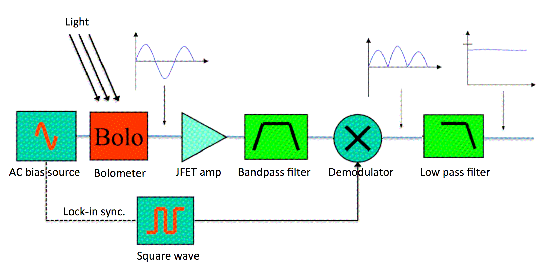
Figure 1: An illustration of the first part of the SPIRE FTS signal chain: The AC signal from the bolometer passes through the JFET amplifier, a bandpass filter that filters out the DC signal, a square-wave amplifier/demodulator that is normally locked in phase with the bolometer bias voltage to turn the negative part of the signal into positive, and finally a low pass filter that generates a slowly varying DC signal. In the bright-source mode, the square-wave demodulator is de-phased from the bolometer signal to further damp the output DC signal.

The overall strategy for the in-flight calibration of the SPIRE FTS is outlined in Swinyard et al. (2010). The actual calibration and pipeline implementation of the FTS nominal mode are described in detail by Swinyard et al. (2013) and Fulton et al. (2013; 2010), respectively. The bright-source mode calibration went through a major upgrade in March 2013 [coinciding with Version 11 of Herschel Interactive Data Processing Environment (HIPE); Ott (2010)]. Prior to HIPE 11, the data of the bright-source mode was processed in the temperature domain, with some residual bolometer nonlinearity passed through to the end of the pipeline. Starting in HIPE 11, we adopted a new full nonlinearity correction scheme and integrated the bright-source mode data processing directly into the existing pipeline for the nominal mode. As a result, the agreement between the bright-source and nominal mode flux calibrations has been improved from within ${\sim}10\%$ in HIPE 10 to within ${\sim}2\%$ in HIPE 11. In this paper, we address those calibration issues unique to the bright-source mode (§2), describe how the data obtained in the bright mode is folded into the nominal-mode pipeline for data processing (§3), demonstrate that the bright-source mode flux calibration accuracy is within about 2% of that of the nominal mode (§4), and finally summarize our results (§5).

2 Calibration Scheme for the Bright-source Mode

The calibration strategy for the bright-source mode is to utilize the calibration products derived for the nominal mode wherever possible, in order to minimize the overall FTS calibration effort and keep the pipeline simple and robust. In this approach, the bright-source mode needs only the following unique calibration products or procedures: (1) a phase-related gain correction factor, $G_{\rm phase}$, for the out-of-phase analog amplifier/demodulator, (2) a detector nonlinearity correction calibration product, (3) a zero-point, DC-type gain correction factor, $G_{0}$, which aligns the linearized signal scale of the bright-source mode to that of the nominal mode, and (4) a possible frequency-dependent gain factor, $G_{f}$. The last one may result from effects such as a dependence of bolometer response time constant on the bias voltage. We address each of these issues in more detail below.

2.1 Phase-related Gain Correction

The square-wave analog amplifier/demodulator is locked in phase with the bolometer AC signal in the nominal mode, but is intentionally kept at $\phi_{\rm diff}$ out of phase in the bright source mode; where $\phi_{\rm diff}$, measured for each detector, varies slightly for different detectors of the same bolometer array, and is around 70 and 68 degrees for SSW and SLW detectors, respectively. As discussed in Swinyard et al. (2013), the effective R-C circuit of the bolometer JFET amplifier and harness introduces a gain factor, $G_{\rm cab}$, and a signal phase shift, $\phi_{t}$, as follows:

$$G_{\rm cab}=\sqrt{{1\over 1+\omega^{2}_{\rm cr}}},$$ (1)

$$\phi_{t}={\rm atan}(\omega_{\rm cr})+\phi_{\rm off},$$ (2)

where $\phi_{\rm off}$ is a constant phase offset ($=11.4$ and $13.6$ degrees for SSW and SLW, respectively) and $\omega_{\rm cr}=2\pi\omega_{\rm bias}R_{\rm tot}C_{\rm H}$, with $\omega_{\rm bias}$ being the detector bias frequency, $R_{\rm tot}$ is the total resistance of the bolometer readout circuit, including the bolometer itself and the load resistors, and $C_{\rm H}$ ($=20\,$pF) is the cable capacitance of the FTS readout system. Since the bolometer resistance depends on the optical load, so does $G_{\rm cab}$. In practice, $G_{\rm cab}$ and $\omega_{\rm cr}$ are determined in an iterative way. The gain factor related to the adjusted phase is given by:

$$G_{\rm phase}=\cos(\phi_{\rm diff}-\phi_{t}).$$ (3)

This $G_{\rm phase}$ is divided into each voltage sample for the bright-source mode at the engineering data conversion stage in the pipeline. Typically, $G_{\rm cab}$ is always close to unity and $G_{\rm phase}$ is on the order of 0.5 (e.g., it is around 0.54 for SSWD4 and around 0.67 for SLWC3).

2.2 Detector Nonlinearity Correction

Since the nonlinear responsivity of a bolometer depends on its bias voltage, it is necessary to derive a separate nonlinearity correction calibration product for each of the two detector-setting modes. For the SPIRE bolometers, the signal linearization can be done in an analytic way as, following Swinyard et al. (2013) and Bendo et al. (2013),

$$V^{\prime}=K_{1}(V_{m}-V_{0})+K_{2}\,\ln({V_{m}-K_{3}\over V_{0}-K_{3}}),$$ (4)

where $V_{m}$ and $V^{\prime}$ are the observed and linearized bolometer voltages, respectively, $V_{0}$ is an arbitrary reference voltage, and $K_{1}$, $K_{2}$ and $K_{3}$ are the parameters characterizing the detector nonlinearity. For the nominal mode, these K parameters were derived from a physical bolometer model (e.g., Sudiwala et al. 2002; Woodcraft et al. 2002) using a bolometer analysis package developed at the NASA Herschel Science Center (Schulz et al. 2005) with both laboratory and in-flight measured detector parameters (Nguyen et al. 2004). For the bright-source mode, which requires nonlinearity correction over a much larger flux range, these K parameters were determined directly from the calibration data taken on flashes of the SPIRE internal photometric calibrator (PCAL; Pisano et al. 2005). Each astronomical FTS observation contains 9 pairs of PCAL flashes on top of the background emission at the position of the target. Some dedicated PCAL calibration observations were also obtained in order to expand the background flux coverage.

For each PCAL flash of power off and power on, we can write

$$1/\delta V_{m}=K_{1}+K_{2}/(V^{\rm off}_{m}-K_{3}),$$ (5)

where $\delta V_{m}$ is the instantaneous bolometer voltage change when the PCAL power is turned on and $V^{\rm off}_{m}$ is the voltage reading just before the PCAL power is turned on. We can write eq. (5) because the PCAL power and illumination pattern remain fixed over the entire mission (as well as between the nominal and bright-source modes) and because an arbitrary common scaling factor is allowed for $K_{1}$ and $K_{2}$. (This scaling factor gets folded into the zero-point gain correction factor in §2.3.)

As examples, Fig. 2 shows two independent sets of PCAL flashes on the detector SSWD4. The left-hand side plot represents a set of PCAL flashes typically seen in an astronomical observation. Note that there is a slight downward signal drift when the PCAL power is on, illustrating a possible heat input to the detectors from the PCAL power. One of our dedicated PCAL calibration observations towards the Galactic center is shown in the right-hand plot to illustrate a typical PCAL observation when the telescope was pointed at a bright discrete source. The strong baseline drift over the on-off cycle was a result of the jitter in the telescope pointing. Our PCAL data reduction pipeline module fit a linear function independently to each on and off signal plateau (after excluding a certain percentage of the data points at the beginning and end of each plateau; see the SPIRE pipeline description document for more details) and determines from these fits $V^{\rm off}_{m}$ and $V^{\rm on}_{m}$ ($=V^{\rm off}_{m}+\delta V_{m}$) per PCAL flash pair. Finally, for each PCAL observation, the median $V^{\rm off}_{m}$ and $\delta V_{m}$ values over all of its PCAL flash pairs were derived for use in our detector nonlinearity characterization.

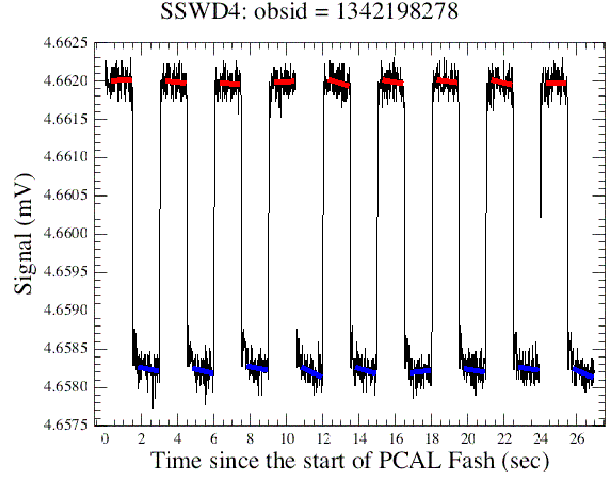
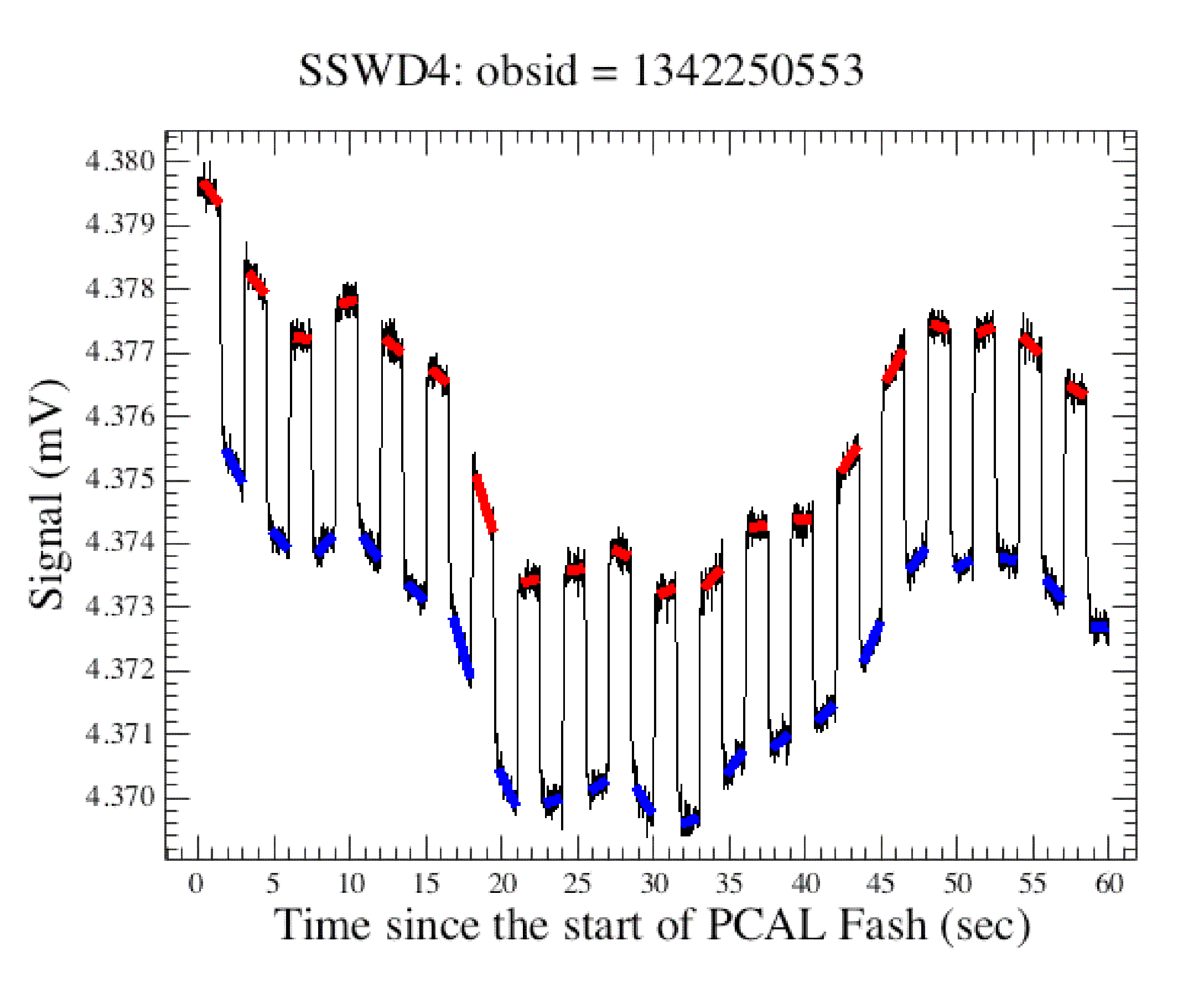
Figure 2: Two examples of PCAL flashes on the detector SSWD4. The actual data samples are shown in black curves. The fits to the power-off and power-on signal plateaus are shown as red or blue lines, respectively.

Fig. 3 illustrates our fitting of eq. (5) to the bright-source mode PCAL data pairs (i.e., $V^{\rm off}_{m}$ and $\delta V_{m}$) we accumulated over the entire mission for the two central detectors, SSWD4 and SLWC3. The voltage coverage along the X-axis ranges from dark sky observations (at the high voltage end) to those from two Saturn observations. It is evident that the data points are still sparse at the low voltage end, leading to possibly a lower flux calibration accuracy for bright targets such as Saturn. For each detector, we defined a voltage range of $V^{\rm off}_{m}{\rm(min)}$ to $V^{\rm off}_{m}{\rm(max)}$, within which the nonlinearity correction based on the fit is deemed to be valid. The value of $V^{\rm off}_{m}{\rm(min)}$ is set to 5% below the smallest voltage sample observed and that of $V^{\rm off}_{m}{\rm(max)}$ to 3% above the largest voltage sample we have. If we compare the PCAL $\delta V$ values on the same background source between the bright-source and nominal modes (for the nominal mode counterpart to Fig. 3 here, see their Fig. 5 in Swinyard et al. 2013), in general, the detector responsivity in the bright-source mode is about a quarter of that in the nominal mode.

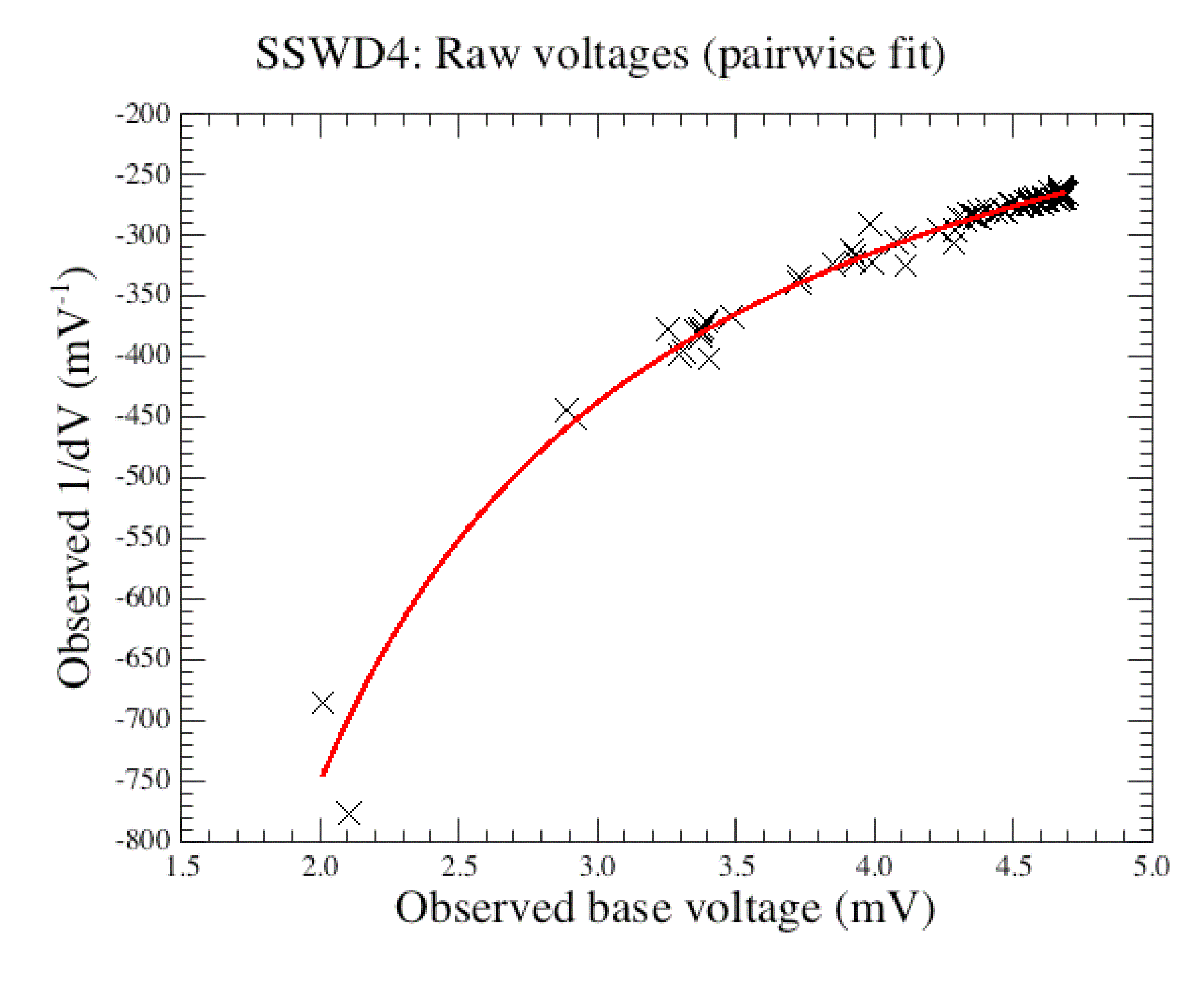
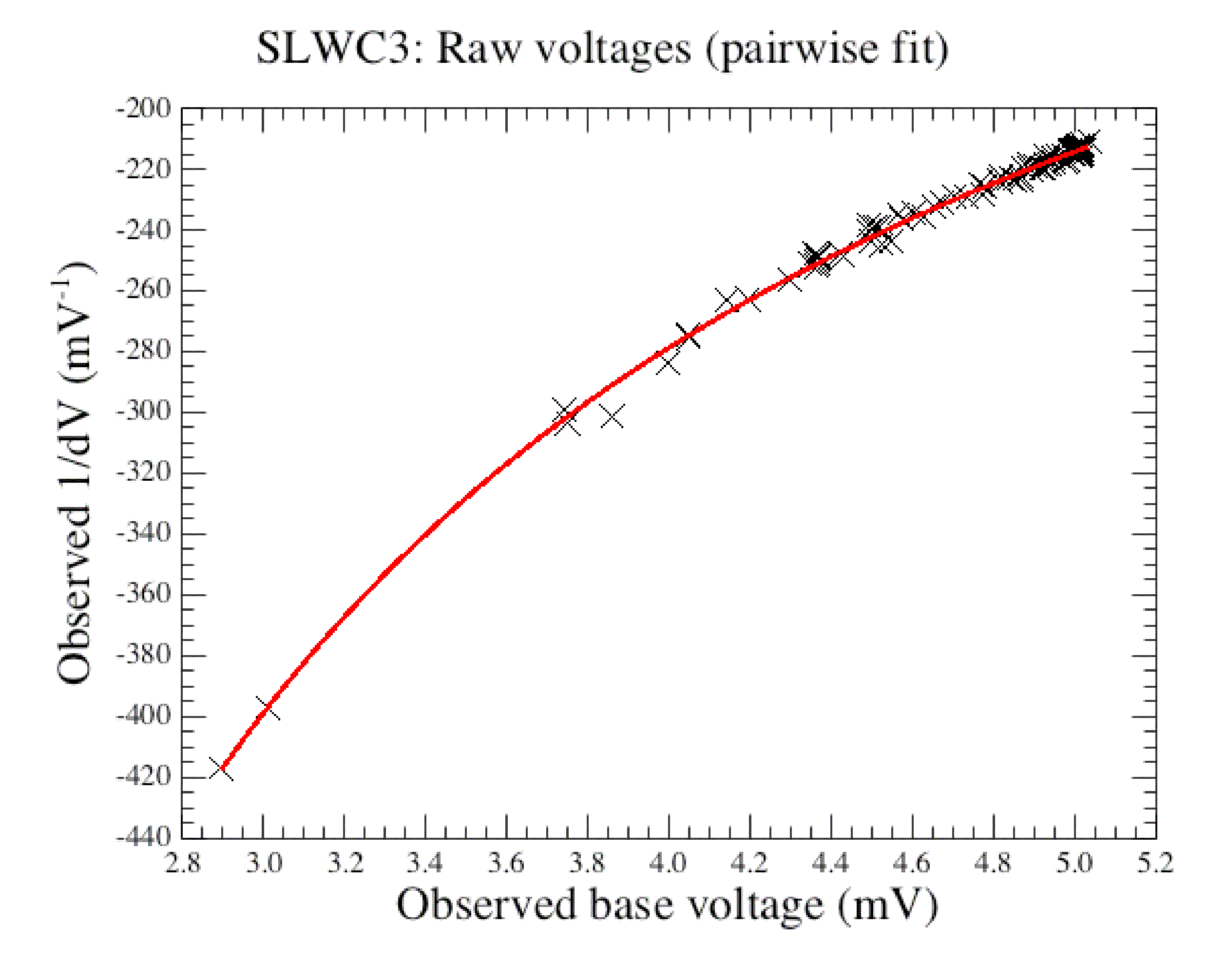
Figure 3: Bright-source mode bolometer nonlinear responsivity fits of eq. (5) to the PCAL data for the two central detectors, SSWD4 (on the left-hand side) and SLWC3 (on the right). The median results from individual sets of PCAL flashes are shown in black crosses. The two data points with the lowest observed base voltages are from PCAL flashes on Saturn. The best fit is shown as a red curve.

2.3 Zero-point Gain Correction

As an example, Fig. 4 shows the linearized PCAL voltages [via eq. (4)] for the detector SSWD4 in the nominal mode (on the left-hand side) and bright-source mode (on the right). These plots also illustrate that, for the majority of the detectors, the typical sample standard deviation for the linearized PCAL signals is of the order of $2\%$ for the bright-source mode and is less than $1\%$ for the nominal mode. Since the linearized voltage is proportional to the optical load on the detector, and the PCAL power and illumination pattern was kept the same for both detector modes, the linearized voltage ratio of the nominal mode to the bright-source mode gives a zero-point gain scaling factor, $G_{0}$, from the bright-source to nominal mode. The resulting $G_{0}$ varies between 4.1 and 5.4, depending on specific detector.

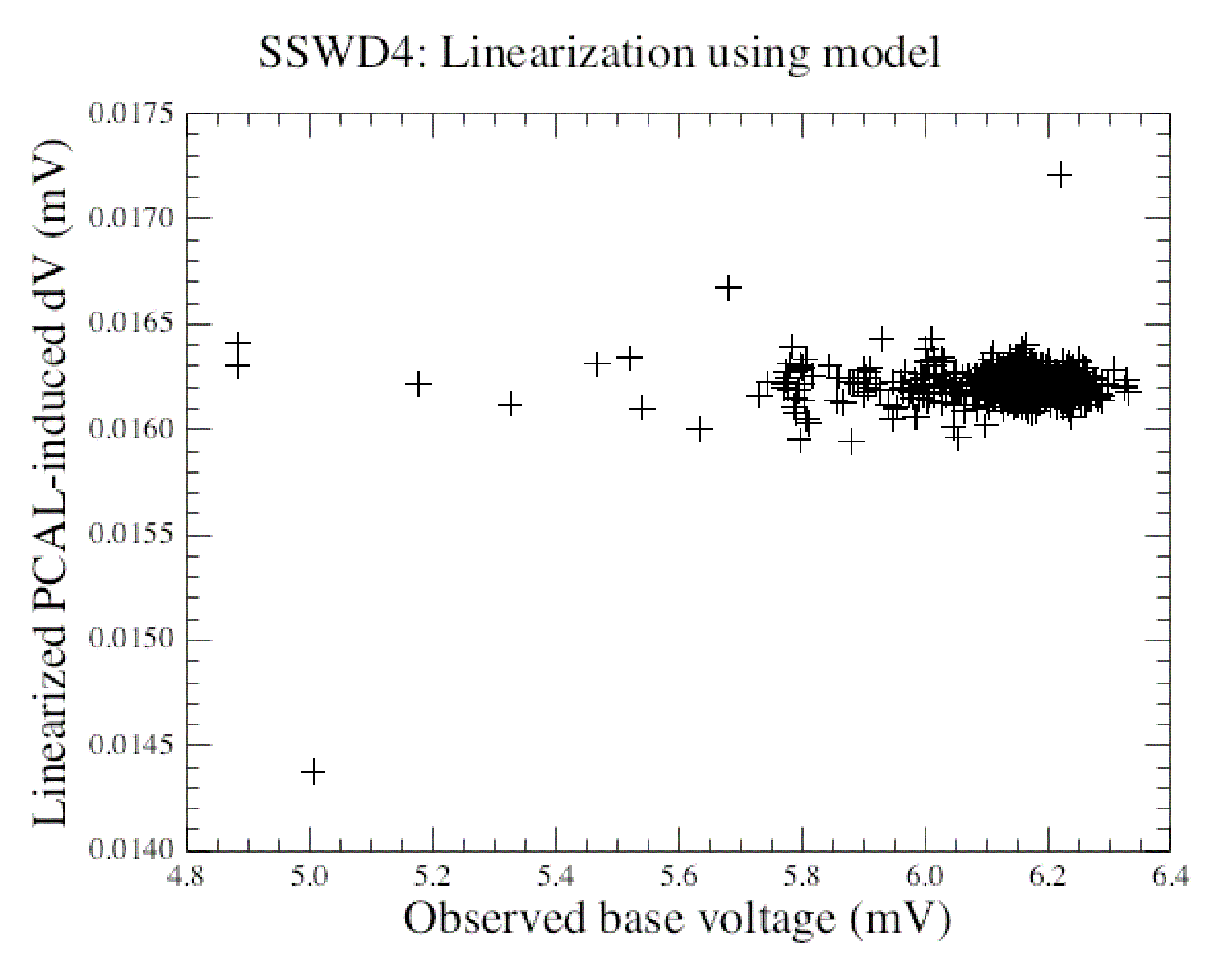
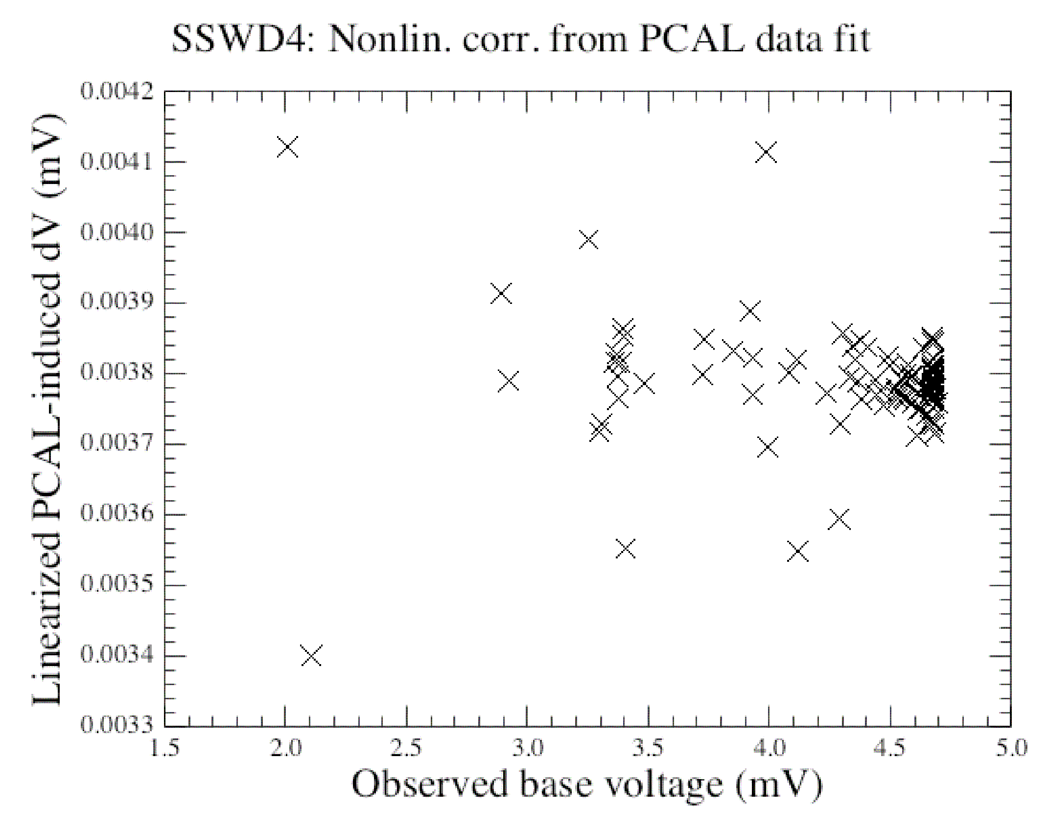
Figure 4: Linearized PCAL signals for the central detector SSWD4, from the nominal model on the left-hand side and from the bright-source mode on the right.

2.4 Frequency-dependent Gain Correction

In addition to $G_{0}$, which was derived from low-frequency PCAL signal time lines, we also expect an additional frequency-dependent scaling factor between the two detector setting modes to account for the higher frequency signal modulations in interferograms. This can arise from the fact that bolometer time constant depends on the bias voltage used. While there is a correction for the finite bolometer time constant implemented in the pipeline, any residual effect from imperfect correction could lead to some spectral shape distortion. In the nominal mode, this potential residual spectral shape distortion is simply corrected for at the flux calibration step in the pipeline. To make use of the same flux calibration product for the bright-source mode, we introduced a frequency-dependent gain factor, $G_{f}$, which is to be applied to bright-source mode spectra.

Fig. 5 shows a number of pair-wise ratios of the nominal to bright-source mode for the two central detectors, SSWD4 and SLWC3, using dark sky spectra taken in the low spectral resolution configuration. Only the zero-point gain correction, $G_{0}$, has been applied to the bright-source data here. Each pair of observations were carried out close in time so that the telescope emission, which dominates the signal observed, remained unchanged over the observational pair. Apart from an increased uncertainty at the low frequency end, where the removal of the instrument emission, which is significant only near that end of SLW, introduces additional flux uncertainties, the ratios show approximately a linear dependence on frequency for each detector array. A linear fit was applied to the data of SSWD4 or SLWC3, resulting $G_{f}$ as a function of frequency. Note that the correction associated with $G_{f}$ is less than ${\sim}5\%$. Similar fits were obtained for all the other detectors.

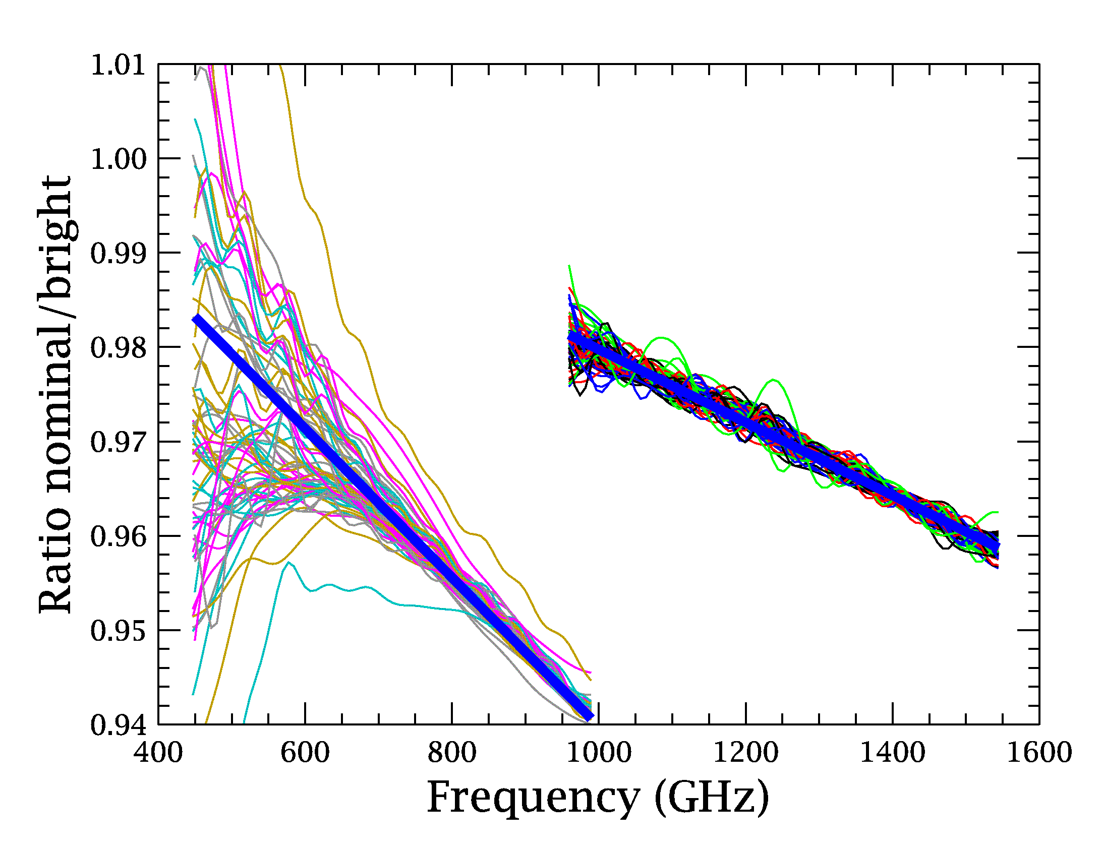
Figure 5: Frequency dependency of pairwise dark spectrum ratios of the nominal mode to the bright-source mode for the two central detectors, SSWD4 and SLWC3. Only the zero-point gain correction, $G_{0}$, was applied to the data of the bright mode here. Independent data pairs are coded in different colors. The spectra have been slightly smoothed in frequency to reduce noise. The two thick blue lines are the best linear fits to the data over SSWD4 and SLWC3, respectively.

3 Pipeline Implementation

Fig. 6 is a flow chart illustration on how the bright-source mode data processing is folded into the standard nominal-mode pipeline. The bright-source mode pipeline processing is the same for the nominal mode except for the following three stages in the pipeline: (a) The phase-related gain correction option is turned on for the bright-source mode at the step of the engineering data conversion. (b) While both detector modes share the sample nonlinearity correction module, they use separate nonlinearity calibration products. (c) After the Fourier transform, there is an extra step for the bright-source mode, i.e., each spectrum is multiplied by a combined gain correction factor, $G_{0}\,G_{f}$, which is a linear function of frequency for each detector.

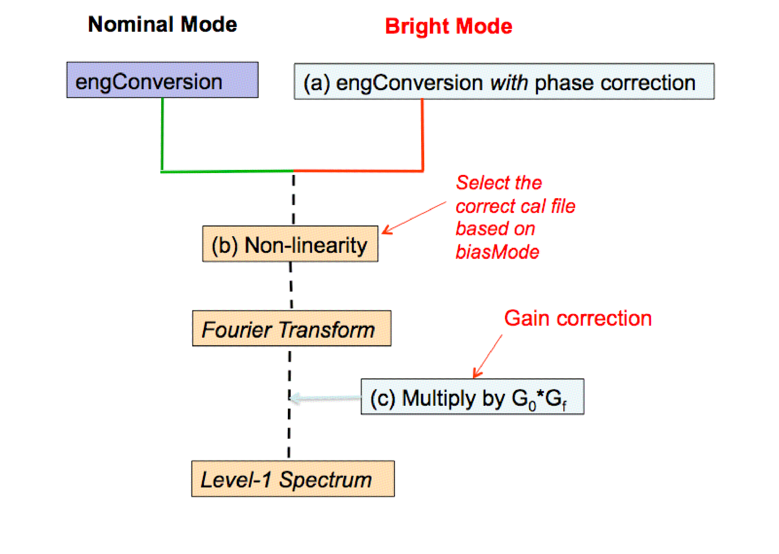
Figure 6: A flow chart illustration on the integration of the bright-source mode data processing into the existing nominal mode pipeline. The three processing stages where the two detector modes are treated differently are marked by (a), (b) and (c), respectively, and are described in the text.

4 Calibration Results

The validity and consistency of the calibration scheme described above can be studied by comparing the bright-source pipeline results with those from the nominal mode for some bright sources that are observable in both observing modes or with independent flux models of very bright celestial standards. Fig. 7 checks the pipeline results of all the high-resolution dark sky observations taken in the bright-source mode over the entire mission. The two central detectors, SSWD4 and SLWC3, are shown here. Individual spectra have been smoothed to reduce effects of noise and fringes. A dark observation is dominated by the warm telescope emission, with an in-beam flux density of ${\sim}200-800\,$Jy over the whole FTS bandwidth. A perfect flux calibration would yield a flat spectrum at 0 Jy for these observations as the telescope emission is removed in the pipeline. It is evident that the mean from these dark sky spectra is close to 0 Jy. The sample standard deviation is of the order of 0.5 Jy, except for the low frequency end of SLWC3 where the scatter is somewhat elevated mainly due to the fact that the removal of the instrument emission, which is significant only near that end of SLW, introduces additional flux uncertainties.

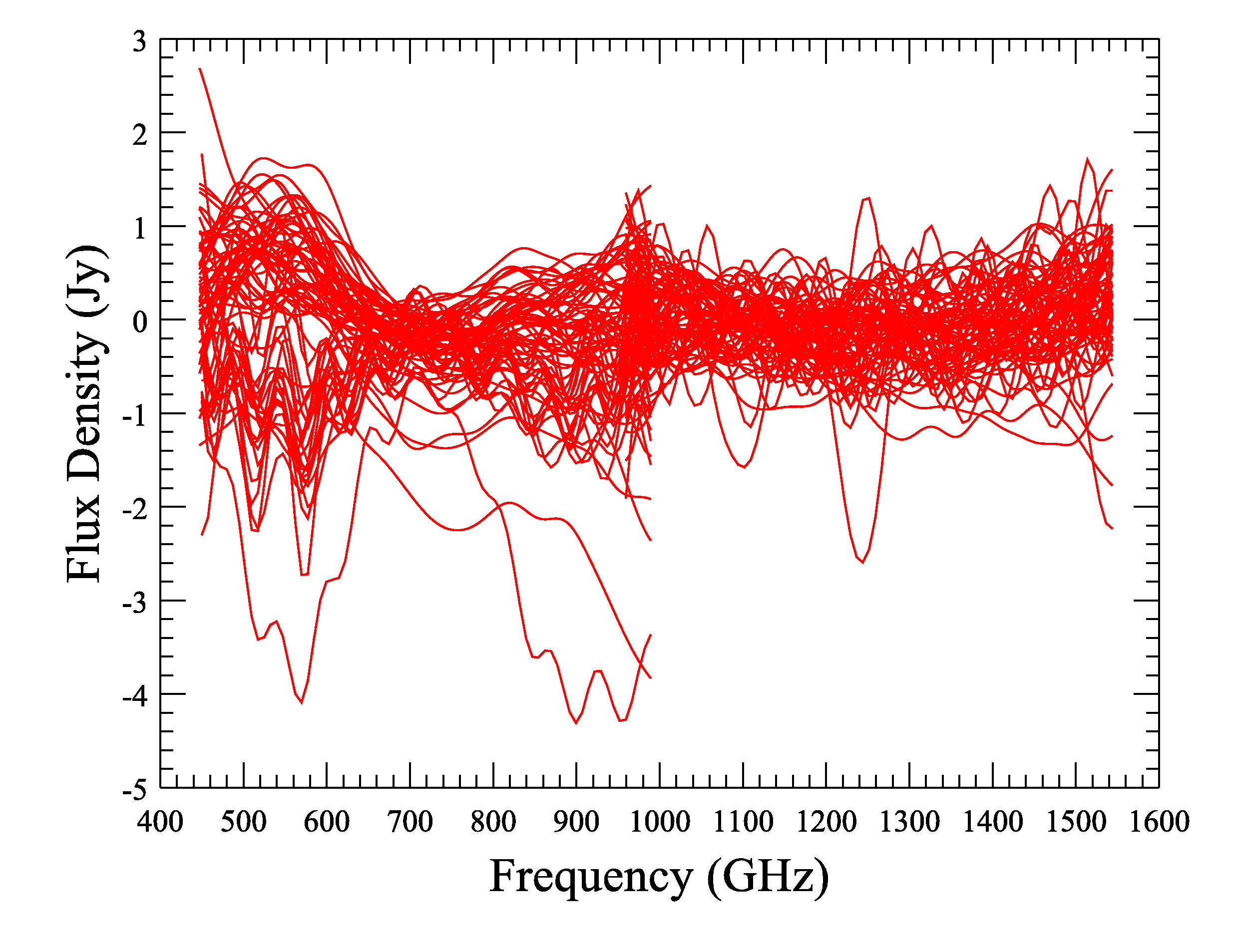
Figure 7: Pipeline spectra of all the high-resolution dark sky observations made in the bright-source mode over the entire mission. Shown here are the two central detectors, SSWD4 and SLWC3. Each spectrum has been smoothed to reduce noise and fringes.

Fig. 8 shows the (smoothed) spectral ratios of the nominal mode to the bright-source mode for a few independent observations of Neptune and Uranus in the central detectors, SSWD4 and SLWC3. Neptune and Uranus are the main photometric flux standards for SPIRE and span a flux-density range from a few tens of Jy to 220 and 500 Jy, respectively, within the SPIRE FTS bandwidth. It is evident that these spectral ratios are all within 2%.

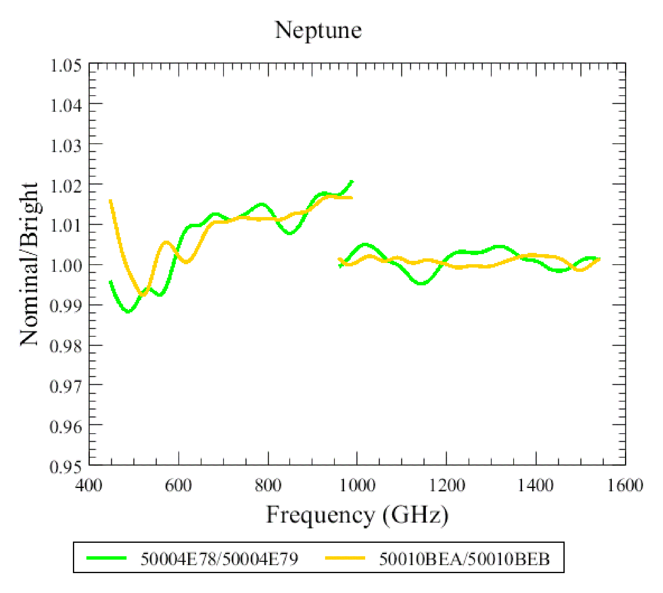
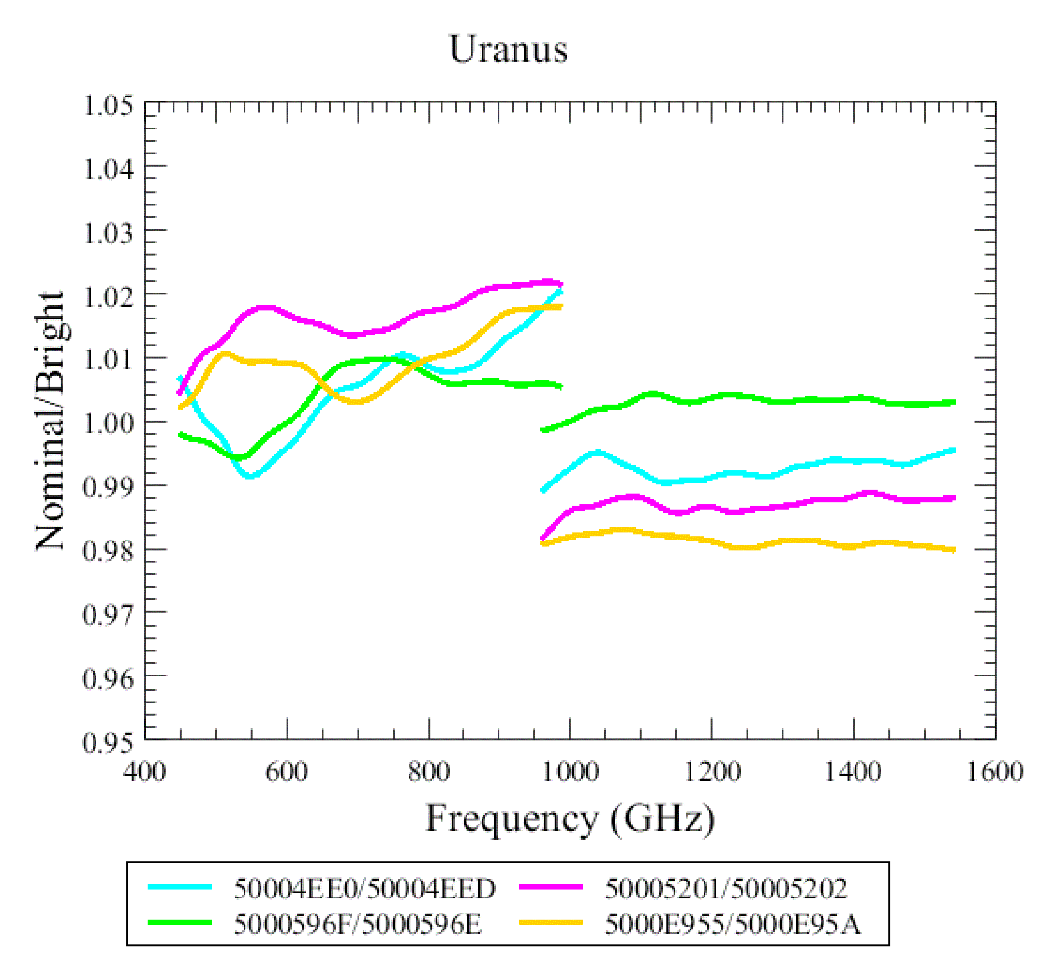
Figure 8: Spectral ratios of the nominal mode to the bright-source mode for a few independent observations of Neptune (on the left-hand side) and Uranus (on the right) in the central detectors, SSWD4 and SLWC3. Individual observations are coded in different colors. All the spectra have been smoothed to reduce noise.

Fig. 9 shows the (smoothed) spectral ratios of the nominal mode to the bright mode for two massive stars, Eta Car and AFGL 2591. Within the SPIRE FTS beams and bandwidth, these two sources span a flux density range from a few tens of Jy to about 600 and 1,000 Jy, respectively. The flux differences between the bright-source and nominal modes are again within about 2% here.

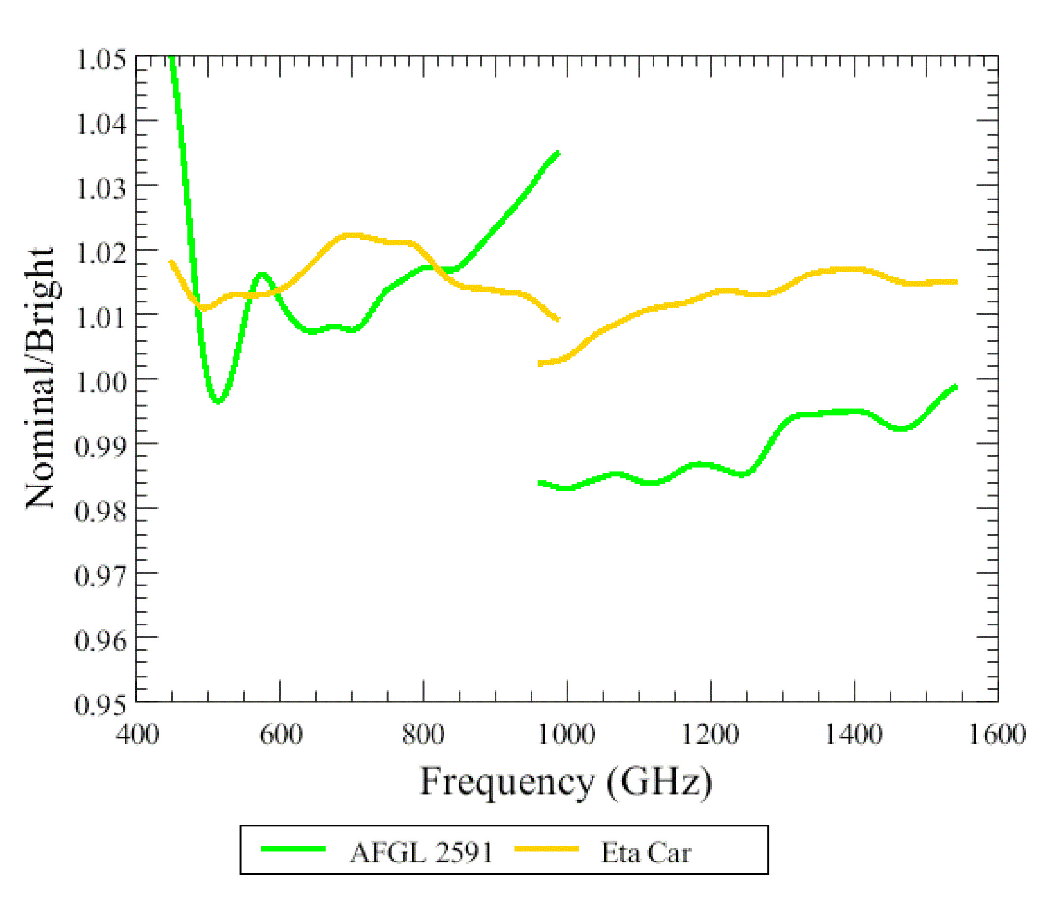
Figure 9: Spectral ratios of the nominal mode to the bright mode for two massive stars, Eta Car (in green color) and AFGL 2591 (in brown), observed in the central detectors SSWD4 and SLWC3. The spectra have been smoothed to reduce noise.

For sources even brighter than those in Fig. 9, there is no longer any nominal mode data for comparison as severe saturation would have occurred. For a few bright planets, there are reasonably accurate model spectra available. We compared our bright-source mode observations with the model spectra for Mars and Saturn. Fig. 10 compares the spectra from three independent, bright-source mode observations of Mars with the model-calculated flux densities at a few selected frequencies. The latter data were derived from an online Mars brightness model provided by E. Lellouch and H. Amri, available at http://www.lesia.obspm.fr/perso/emmanuel-lellouch/mars/. For the three observations, Mars was at different distances, hence had different apparent diameters (given in the figure caption) and fluxes. The SPIRE spectra have been corrected for a finite angular size appropriate at the time of the observation, using the SPIRE semi-extended source correction tool (Wu et al. 2013). The agreement with the model fluxes is generally good to within a few percent.

The recommended flux density limit for the nominal mode is ${\sim}500\,$Jy, or roughly ${\sim}$1,000 Jy including the telescope background. The bright-source mode suppresses voltage signals by a factor of ${\sim}8$ (with a factor of ${\sim}2$ from the de-phased amplifier and a factor of ${\sim}4$ from the reduced detector responsivity). The corresponding targeted upper flux density limit for the bright-source mode is therefore on the order of 7,500 Jy ($=8\times$1,000 Jy less $500\,$Jy of the telescope background). This is comparable to the flux density of Mars in Fig. 10 and encompasses the range seen in the vast majority of the bright-source mode science observations. Only a few objects brighter than Mars, such as Saturn, were ever observed during the entire mission.

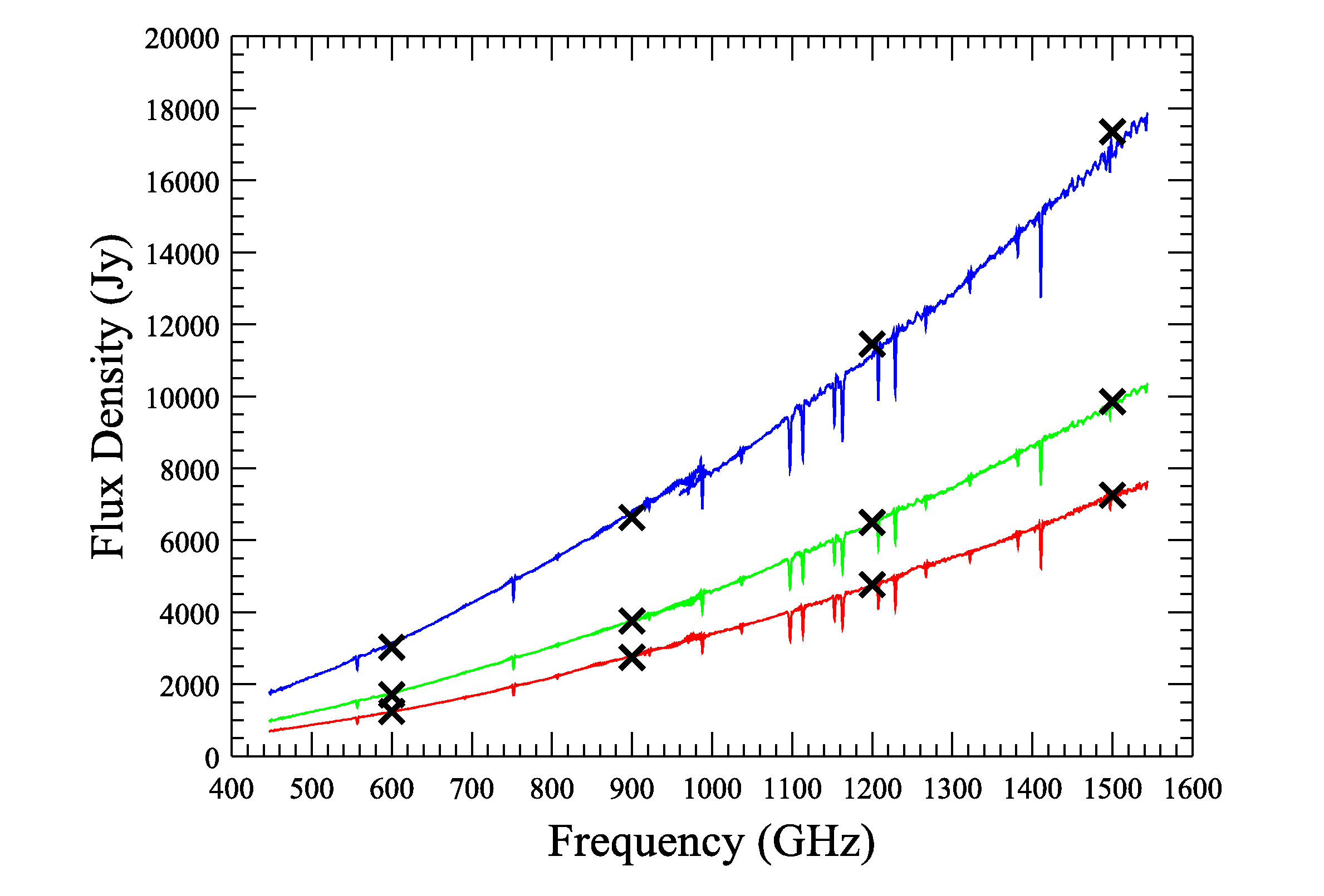
Figure 10: Comparison of the spectra from three independent bright-mode observations of Mars with the model predicted flux densities (crosses) at a few selected frequencies. The three observations are identified by the following obs. ID: 0x5000D22D (or 1342231085; red curve, the angular size used is $\theta=5.5^{\prime\prime}$), 0x50011293 (or 1342247571; green curve, $\theta=6.6^{\prime\prime}$), and 0x50010BD8 (or 1342245848; blue curve, $\theta=8.8^{\prime\prime}$). Each SPIRE spectrum has been corrected for the finite angular size, $\theta$, of Mars appropriate at the time of the observation using the SPIRE semi-extended source correction tool.

Fig. 11 compares an observed SPIRE FTS spectrum in the bright-source mode with a model spectrum for Saturn. The model spectrum is from Fletcher et al. (2012) after scaling their spectrum to the angular size ($=17.4^{\prime\prime}$) of Saturn at the time of our bright-source mode observation. Saturn is so bright that its induced bolometer voltages are at the low voltage end of the calibrated range for the detector nonlinearity correction, and its flux levels are significantly above the targeted upper flux density limit for the bright-source mode. The flux calibration in this case is likely less accurate than in those of typical bright-source mode observations (i.e., fluxes up to that of Mars). Nevertheless, the largest flux discrepancy in Fig. 11 is still less than 10% at such extreme flux levels. A few other independent Saturn observations also confirm a flux uncertainty of less than 10%.

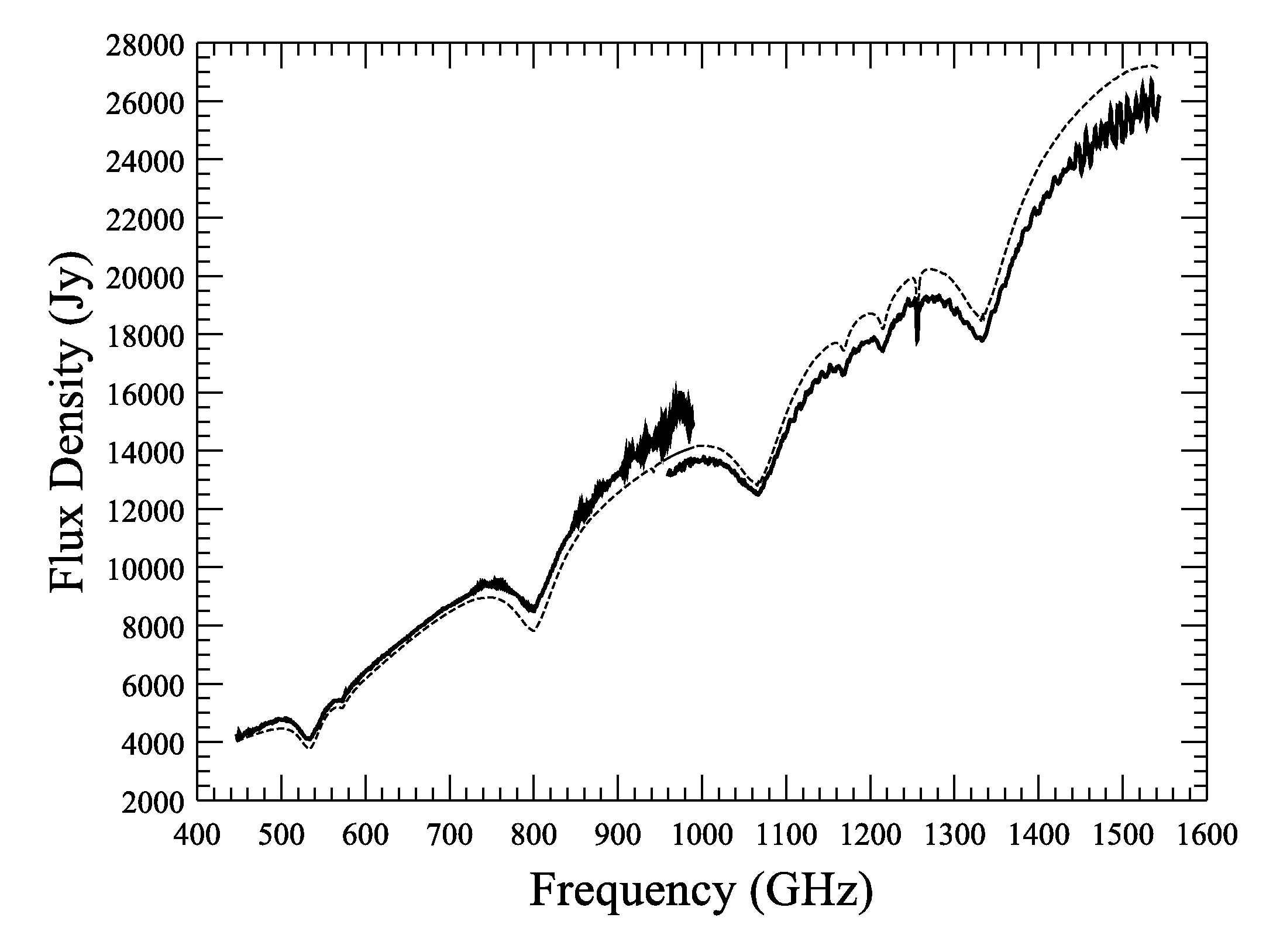
Figure 11: Comparison of an observed spectrum (obs. ID = 0x50011346 or 1342247750; thick curve) of Saturn with the model predicted spectrum (thin, dashed curve). The SPIRE spectrum has been corrected for a finite angular size of $17.4^{\prime\prime}$ for Saturn at the time of the observation, using the SPIRE semi-extended source correction tool.

Finally, Fig. 12 shows the average sensitivity ratio of the bright-source mode to the nominal mode, based on the dark observations taken post Operational Day 1011. The sensitivity prior to that day is very similar. This sensitivity was derived from the observed spectral noise of the dark observations. For each dark spectrum, the 1-$\sigma$ r.m.s. noise was calculated within each and every spectral bin of 50 GHz. The noise of a specific spectrum was further normalized to a reference integration time before the average sensitivity was finally calculated for each observing mode. The results show that the bright-source mode is about 3 to 4 times less sensitive than the nominal mode.

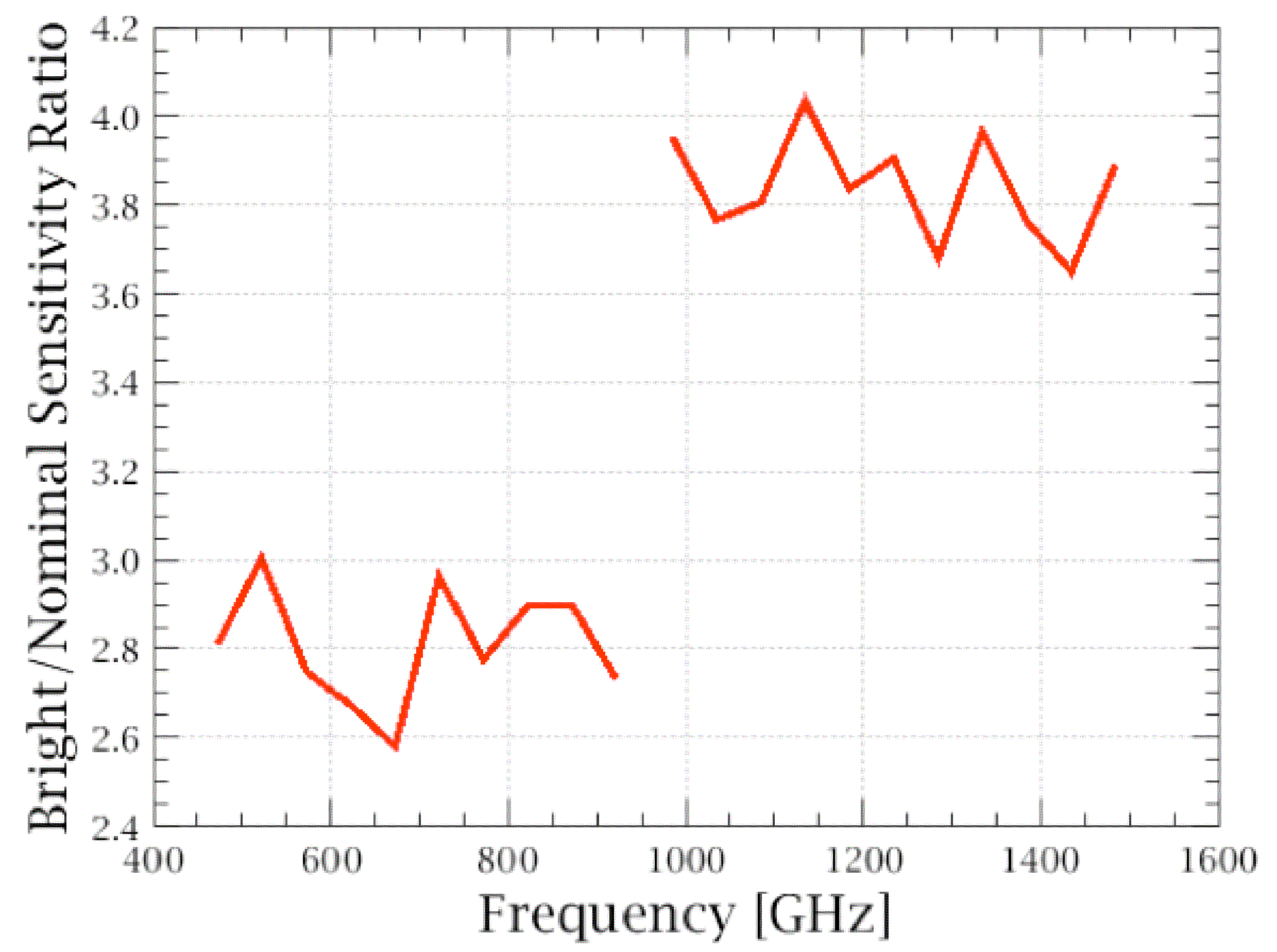
Figure 12: Average sensitivity ratio of the bright-source mode to the nominal mode, based on all the dark observations post Operational Day 1011. It shows that the bright-source mode is about 3 to 4 times less sensitive than the nominal mode.

5 Summary

SPIRE spectrometer bright-source mode calibration went through a major upgrade in March 2013 [i.e., starting in Herschel Interactive data Processing Environment (HIPE), version 11], by adopting a full nonlinearity correction scheme and integrating its data processing into the existing data processing pipeline of the nominal detector mode. This simplified data processing scheme requires only one additional phase-related gain correction procedure and two calibration products unique to the bright-source mode: a nonlinearity correction product and a frequency-dependent, composite gain correction. The derivations of these calibration products were given in this paper. We have demonstrated that the bright-source mode flux calibration is within ${\sim}2\%$ of that of the nominal mode for their overlapping flux range, and agrees within a few percent with the model spectrum of Mars at flux levels as high as ${\sim}$10,000 Jy, which is close to the targeted upper flux density calibration for the bright-source mode. This represents a clear improvement over the 10% flux consistency between the two detector modes achieved in the earlier calibration versions (i.e., HIPE 9 and 10). We showed that the bright-source mode sensitivity is about 3-4 times less than that of the nominal mode.

- (1) Bock, J. J., Glenn, J., Grannan, S. M., Irwin, K. D., Lange, A. E., Leduc, H. G., Turner, A. D.: Silicon nitride micromesh bolometer arrays for SPIRE, SPIE 3357, 297-304 (1998)
- (2) Fletcher, L. N., Swinyard, B., Salji, C., et al.: Sub-millimtre spectroscopy of Saturn’s trace gases from Herschel/SPIRE, A&A, 539, 44 (2012)
- (3) Fulton, T. R., Baluteau, J.-P., Bendo, G., et al.: The data processing pipelines for the Herschel/SPIRE imaging Fourier transform spectrometer, SPIE, 7731, 99 (2010)
- (4) Fulton, T., et al.: The data processing pipeline for Herschel SPIRE Fourier transform spectrometer, A&A, in preparation (2013)
- (5) Griffin, M. J., Abergel, A., Abreu, A., et al.: The Herschel-SPIRE instrument and its in-flight performance, A&A, 518, L3 (2010)
- (6) Nguyen, H. T., Bock, J. J., Ringold, P., et al.: A report on the laboratory performance of the spectroscopic detector arrays for SPIRE/HSO, Proc. SPIE 5498, 196 (2004)
- (7) Ott, S.: The Herschel data processing system - HIPE and pipelines - up and running since the start of the mission, ASPC, 434, 139 (2010)
- (8) Pilbratt, G. L., Riedinger, J. R., Passvogel, T., et al.: Herschel Space Observatory. an ESA facility for far-infrared and submillimeter astronomy, A&A, 518, L1 (2010)
- (9) Pisano, G., Hargrave, P., Griffin, M., Collins, P., Beeman, J., & Hermoso, P.: Thermal illuminators for far-infrared and submillimeter astronomical instruments, Appl. Opt., 44, 3208 (2005)
- (10) Schulz, B., Bock, J. J., Lu, N., et al.: Noise performance of the Herschel-SPIRE bolometers during instrument ground tests, SPIE, 7020, 52 (2008)
- (11) Schulz, B., Zhang, L., Ganga, K., Nguyen, H., Holmes, W.: An analysis package for bolometer ground testing, ASPC, 347, 158 (2005)
- (12) Sudiwala, R. V., Griffin, M. J., Woodcraft, A. L.: Thermal modeling and characterization of semiconductor bolometers, Int. Journal of Infrared and Mm Waves, 23, 545 (2002)
- (13) Swinyard, B. M., Ade, P., Baluteau, J.-P., et al.: In-flight calibration of the Herschel-SPIRE instrument, A&A, 518, L4 (2010)
- (14) Swinyard, B. M., Polehampton, E. T., Hopwood, R., et al.: Calibration of the Herschel SPIRE Fourier transform spectrometer, MNRAS, in preparation (2013)
- (15) Woodcraft, A. L., Sudiwala, R. V., Griffin, M. J., et al.: High precision characterisation of semiconductor bolometers, Int. Journal of Infrared and Mm Waves, 23, 575 (2002)
- (16) Wu, R., Polehamption, E. T., Etxaluze, M., et al.: Observing extended sources with the Herschel SPIRE Fourier transform spectrometer, A&A, 556, 116 (2013)