Variance-based control of regime shifts: bistability and oscillations

Abstract

A variety of real world and experimental systems can display a drastic regime shift, as the evolution in one its paramaters crosses a threshold value. Assimilation of such a transition with a bifurcation has allowed to identify so called “early warning signals”, at the level of the time series generated by the system underscope. The literature in early warning detection methods is currently expanding and their potential for practical applicability is being discussed in different contexts. In this work, we elaborate on the use of the variance of a system variable, which constitutes the simplest early warning indicator, to gain control on the long-term dynamics of the system, while extending an exploitation phase. In particular, we address the cases of the cusp and Hopf normal forms, as prototypical examples of bistability and oscillations. Our results provide insights on the interplay between the time-scale for the system observation, the degree of sensitivity of the control feedback and the intensity of the random perturbations, in shaping the long-term control efficiency.

I Introduction

Along the last few decades an increasing number of scholars has been contributing to develop a coherent and further integral body of knowledge on complex real world systems. Cross-fertilization of concepts and tools stemming from dynamical systems, statistical physics and information and computation theories has allowed to identify and analyse systems whose observable behaviors result from similar underlying mechanisms NicolisI ; Politi . As a result of these attempts, a key finding has been realization of the ubiquity of nonlinear feedbacks in the dynamics of different classes of systems.

In particular, the occurence of drastic, qualitative shifts of the functioning regime of systems –as resulting from strong positive and negative feedbacks– has attracted interest in diverse research fields, as diverse as microscopic physical systems at equilibrium Stanley and their macroscopic non-equilibrium counterpart NicolisII ; Cross , ecology SchefferIV ; Scheffer , socio-physics Castellano and Earth system science Lenton ; Scheffer .

Insights into the phenomenology, related to regime shifts and the development of new methods for their early detection, have relied on minimal models. A frequent idea in this approach is to cast the description of the system evolution as a stochastic differential equation Gardiner , of the form:

$$\textbf{dx}=\textbf{F}(\textbf{x},\lambda)dt+d\textbf{$\textbf{W}_{x}$}$$ (1)

The key variables of the system are represented as a vector $\textbf{x}=(x_{1},x_{2},\dots,x_{N})$ and their dynamic interrelationships are considered as deterministic laws, described as a vector field F. Vector $\textbf{W}_{x}$ aims at introducing the effect of incessant perturbations on the x components, as typically resulting from endogenous meso-scale dynamic complexity and from an infinite number of uncorrelated environmental factors. Consequently, $\textbf{W}_{x}$ is assimilated to a Gaussian Wiener process Gardiner with standard deviation $\omega_{x}$. The parameter $\lambda$ controls the qualitative behavior of solutions to the deterministic part of system (1) around a stationary state $\textbf{x}_{s}$. In this framework, a regime shift is represented as a local bifurcation occuring in the deterministic part of the system at a critical point $(\textbf{x}_{s},\lambda_{c})$, i.e., that the Jacobian matrix of F, evaluated at $\textbf{x}_{c}$, possesses one eigenvalue whose real part tends to zero as $\lambda$ approaches the value $\lambda_{c}$ Guckenheimer . Thereby, the response of the system to random fluctuations can be studied along the evolution towards the bifurcation point.

Given the relevance of applications and implications of regime shifts in real world systems, it is of increasing interest to construct early warning indicators (EWI) SchefferI ; SchefferII – with focus on identifying statistical signatures of the loss of stability in the time series generated by the evolution of the system towards criticality. Conjointly, a relevant phenomenon is the slowing down of the fast stabilizing dynamic modes –often referred as critical slowing down. This results from the real part of the leading eigenvalue becoming zero as the system closely approaches the bifurcation point SchefferI .

As illustrated in a pioneering work by S. Carpenter Carpenter on EWI-based monitoring of shallow lake ecosystems, the onset of the critical slowing down can lead to a drastic increase in the variance of a variable of the system. More recently, the skewness Guttal , kurtosisBiggs and the autocorrelation function Livina of a system variable have been shown to capture relevant information on the increased loss of stability close to the bifurcation point.

The literature in early warning detection is rapidly expanding and their potential applications within a broad range of real world problems is being discussed SchefferI ; SchefferII . Within this contextual frame, it becomes natural to inquire about the possible long-term complex behavior that would arise if EWIs are repeatedly used to control systems potentially undergoing regime shifts. As far as we know, this question remains open, in the light of earlier and further recent advanced methods in the construction of EWI’s Dakos .

In order to tackle this question, we propose to analyze the dynamics of a system represented by (1) subject to a control process. The basic idea is that such a steering control should: 1) re-establish the stability of the system before it crosses a critical point, or 2) re-establish a lost initial system regime once a critical point has been crossed, to then let the system evolve again towards criticality.

Let us explore this idea by considering a control system which reacts upon the behavior of an EWI, denoted by $I_{\tau}$, whose construction is based on information about the past states of the system within a sliding observation time window of size $\tau$. In other words, we are interested in analyzing the coupled dynamics of (1) with an evolution equation for $\lambda$, of the form

$$d\lambda=\Phi(I_{\tau},\alpha)dt+dW_{\lambda}$$ (2)

Here we require the control functional $\Phi$ to operate a change of sign, at the level of $d\lambda$, once $I_{\tau}$ crosses a reference value $V_{R}$. In order to allow for differences in the degree of sensitivity of the control system, let us consider the control response to changes in the ratio $I_{\tau}/V_{R}$ as modulated by a parameter $\alpha$. Moreover, let us assume that the control response may exhibit random variability as a result of the influence of many uncorrelated factors. Thus, we denote by $W_{\lambda}$ a Gaussian Wiener process with standard deviation $\omega_{\lambda}$.

In the domain of application of EWIs, relevant cases are those where the control variable $\lambda$ is driven by human interventions. In many of these instances, the evolution of the system towards criticality is the result of an “exploitation” process, that is sought to be intensified and mantained, while avoiding a system regime shift. Consider for instance catching rates in sustainable fisheries Ray , agriculture related leaching rates of phosphorus into a shallow lake, whose oligotrophic regime is to be preserved SchefferIII , or the increase in the autocatalytic production of chemical species in a well-stirred reactor NicolisIII , where a low entropy production regime may be desirable. Consequently, we characterize the dynamics of system (1)-(2) in terms of two phases: exploitation if $\Phi>0$ and recovery if $\Phi<0$.

Central questions for us are:

• The role of the time-scale $\tau$, considered for the construction of the EWIs, in shaping the emergence of control properties in a system (1)-(2).

• The long-term complex dynamics that can result from the temporal non-locality introduced by the EWI into the dynamics of the coupled system (1)-(2). In other words, in the long-term, the control exerts changes on the system on the basis of the past dynamics of the system and its control as a whole. This opens the possibility to observe different complex behaviors, as the effective dimension of the system-control is augmented by its dependency on the past.

• The efficiency of the control process in terms of: its capacity to increase and mantain explotation in a selected regime as a function of the observation window $\tau$, of the control response sensitivity $\alpha$ and of the variance of stochastic perturbations $\omega_{x}$ and $\omega_{\lambda}$.

In Sec.II we address these questions, by exploring numerically the performance of control on minimal dynamical systems of generic character, that reproduce the prototypical phenomena of bistability and oscillations. Each of these controlled systems is first studied in absence of noise, in order to reveal the role of the observation time scale in shaping the leading deterministic dynamics. Upon the basis of the insights thereby generated, for each system, we introduce a suitable measure of control efficiency. Subsequently, we address the influence of the variance of noise, for different observation time windows and different degrees of control response, on the efficiency of both systems under consideration. Finally, in Sec.III we summarize our main results and conclusions.

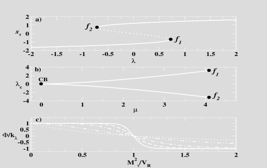
Figure 1: a) plot of a fold bifurcation diagram, as provided by the stationary solutions of the cusp normal form 5, as a function of parameter $\lambda$ and for $\mu=3/2$. The solid lines correspond to the stable branches and the dashed line to the unstable one. Unstable and stable branches meet and anhihilate each other at the saddle-node bifurcation points $f_{1}$ and $f_{2}$; b) plot of the branches formed by the critical values of $\lambda$ corresponding to both $f_{1}$ and $f_{2}$ bifurcation points, as a function of a second parameter $\mu$. Both branches converge to the cusp bifurcation point CB at $\mu=0$. Finally, plot $\Phi/k_{\lambda}$ vs $M^{2}_{\tau}/V_{R}$, for $\alpha=1$ (dot), $\alpha=2$ (dot-dot-dash), $\alpha=5$ (dot-dash), $\alpha=10$ (dash) and $\alpha=20$ (solid).

II Normal forms and control

Regardless of the complexity of its dynamics, as a system evolves further into the vicinity of a bifurcation point, there is a decrease in the number of degrees of freedom necessary to effectively describe the dynamics. This remarkable fact can be understood as a direct consequence of the gradual run out of the fast-relaxation dynamic modes that occurs along with the critical slowing down. A corner stone in local bifurcation theory is the application of the centre manifold method Guckenheimer to identifying canonical descriptions of the nonlinear behavior around a bifurcation point, in terms of a reduced number of variables that contain the whole information about the dynamics of the slow leading modes. Such simple representations –so called normal forms– describe the long-term behavior of the normalized amplitude of the stable solutions that emerge at criticality. The importance of normal forms lies on the fact that the dynamics of different types of systems, around the critical point, can be mapped one-to-one continuously onto the one displayed by a normal form NicolisIV . This property –known as topological equivalence– allows to define classes of universality, where near the critical point, the dynamics of systems belonging to the same class can be mapped onto each other by a change of variables preserving the direction of trajectories. Naturally, a simple and most representative element in a class of universality is thus the corresponding normal form.

With the aim of tackling questions i)-iii) above in a general context, we shall focus our analysis of control dynamics on selected normal forms. As an EWI we consider the variance $M^{2}_{\tau}[\delta x_{j}]=\frac{1}{\tau}\int_{t-\tau}^{t}(\delta x_{j}(t^{\prime}))^{2}dt^{\prime}$ of deviations of a system variable around its mean value, within the time window $\tau$, i.e. $\delta x_{j}=x_{j}-\frac{1}{\tau}\int_{t-\tau}^{t}x_{j}(t^{\prime})dt^{\prime}$. Consistently with the minimal character of the normal form description, let us consider a simple expression for the control functional in (2), of the form

$$\Phi(\tau,\alpha)=k_{\lambda}\Bigg{(}1-2\frac{M_{\tau}^{2}[\delta x_{j}]^{\alpha}}{M_{\tau}^{2}[\delta x_{j}]^{\alpha}+V_{R}^{\alpha}}\Bigg{)}\mbox{, $k_{\lambda},\alpha>0$}$$ (3)

where $k_{\lambda}$ corresponds to the maximum exploitation and recovery rates. For low values in $\alpha$ both the exploitation and recovery phases develop weakly as $M_{\tau}^{2}[\delta x_{j}]$ crosses the threshold value $V_{R}$. As $\alpha$ is arbitrarily increased, the functional $\Phi$ sharply approaches a Heavyside function (see (Fig.(1)c)) –which emulates a full blown response of the control system (2) to a threshold overshooting

$$\Phi(\tau,\alpha\rightarrow\infty)=\left\{\begin{array}[]{c l}k_{\lambda}&\mbox{$\frac{V_{R}}{M_{\tau}^{2}[\delta x_{j}]}>1$}\\ \\ 0&\frac{V_{R}}{M_{\tau}^{2}[\delta x_{j}]}=1\\ \\ -k_{\lambda}&\mbox{otherwise}\end{array}\right.$$ (4)

Here, a comment is in order with regard to the choice of the variance of a system variable as an EWI. As discussed in DakosI , in the more general case where the standard deviation of the random perturbations is a time dependent function, the variance of a system variable may not constitute a reliable EWI. Consequently, we shall restrain ourselves to the case where both standard deviations $\omega_{x}$ and $\omega_{\lambda}$ in (1)-(2) are constants.

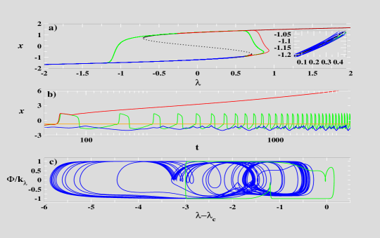
Figure 2: For $\tau=10$ (red), $\tau=11$ (green) and $\tau=35$ (blue), a) plot of a CCS deterministic trajectories ($\omega_{x}=0,\omega_{\lambda}=0$) in the ($\lambda,x$)-plane (in black lines the bifurcation diagram of the cusp normal form); b) plot x vs time (in orange the critical value $x_{c}$) and c) Plot of $\Phi/k_{\lambda}$ vs $\lambda-\lambda_{c}$, as related to the system trajectories in panels a) and b), for $\tau=11$ and $\tau=35$. Here, values $\Phi>0$ and $\Phi<0$ are considered as exploitation and recovery, respectively. Parameters and initial condition: $\mu=3/2$, $k_{\lambda}=1/10$, $\alpha=2$, $V_{R}=1/100$. $x(0)=-3/2$, $\lambda(0)=-5$. Time step $dt=5\times 10^{-3}$, numerical integration over $5\times 10^{5}$ time steps.

II.1 The cusp-control system (CCS)

As pointed out in SchefferI ; Hastings , the phenomenology observed in so called catasrophic regime shifts in different types of systems can be suitably assimilated with a saddle-node bifurcation. As a parameter evolves, a saddle-node bifurcation occurs when a stable (node) and an unstable (saddle) fixed point solution, to the deterministic evolution law of the system, approach each other and anhihilate upon meeting. This entails the destabilization of the system, which is thus led to an abrupt runaway –this constitutes a catastrophic regime shift. However, since in real systems unbounded runaways are ruled out, saddle-node bifurcations are typically found in cases where the branch formed by the system fixed points folds upon itself, within a range of values in the control parameter $\lambda$ (see Fig.1a). The presence of such a folding entails the existence of a region where two stable solution branches coalesce along with an unstable one. In this picture, the unstable branch marks the boundary line between the two basins of attraction, associated to both stable branches. In general, the distance between the bifurcation points at the extremes of the s-shape folding ($f_{1}$ and $f_{2}$ in Fig.1b) is determined by a second paramater $\mu$. Examples of such a bistability are reported in different types of systems, ranging from laser and cell division, to ecoystems and climate SchefferI .

In order to explore the question of bifurcation control in the context of bistability, let us consider the cusp normal form

$$F(x,\lambda)=x(\mu\pm x^{2})+\lambda$$ (5)

The solutions to the stationary form $F(x_{s},\lambda)=0$ (with the sign minus in (5)), as a function of $\lambda$, correspond to those plotted in Fig.1a. The position of the saddle-node bifurcation points $f_{1,2}$ are determined by the relation $f_{1,2}=\{(\lambda,\mu)|\lambda=\pm\frac{2}{3\sqrt{3}}\mu^{3/2}\}$. Accordingly, both branches approach each other and merge as $\mu$ tends to zero, at the so-called cusp bifurcation point (Fig.1b). A similar behavior occurs when changing the sign in the second term in (5), which amounts to inverting the s-shaped folding.

We carry out the numerical integration of the variance-based cusp-control system (CCS) (1), (2), (3 and 5) via a standard Euler-Maruyama approximation Gardiner .

II.1.1 CCS deterministic dynamics

In order to illustrate the dynamics of the CCS in absence of noise ($\omega_{x}=0,\omega_{\lambda}=0$), let us consider exploitation as initially occuring along the negative branch in Fig.1a, a moderate degree of control response $(\alpha=5)$ (see Fig.1c) and a small variance reference threshold $V_{R}=1/100$.

According to the numerical results, we distinguish three basic long-term CCS behaviors:

• Exploitation runaway: If the time window is small as compared to a critical value $\tau_{c}$, the system crosses the bifurcation point $f_{1}$ and a regime shift occurs. As the system is expelled onto the upper branch, the control mechanism reacts to the overshooting of the reference value $V_{R}$. This triggers a recovery stage ($\Phi<0$) along the upper branch. However, as the system evolves along the upper branch, it eventually losses completely the “memory” on the original low branch regime. As a result, the variance decreases gradually below $V_{R}$, recovering is interrupted and the CCS switches to runaway explotation (red lines in Figs.2a,b).

• Hysteretic pathways: When the observation window is now greater than the critical value $\tau_{c}$, a transition occurs, from runaway exploitation to long-term control. For specific $\tau$-ranges, the system crosses the bifurcation point $f_{1}$ and it starts recovering along the upper branch. However, differently from B1, the upper branch recovering continues further and the bifurcation point $f_{2}$ is crossed. Thus, the system undergoes again a regime shift towards the original lower branch. As the system stability increases and information about the upper branch is lost, the CCS eventually switches to exploitation, beyond $f_{1}$ (green lines in Figs.2a,b). This exploitation-recovery process is mantained in the long-term. Processes describing cycles along the zone of bistability are commonly refered as hysteretic. Figure 2c depicts the long-term hysteretic exploitation-recovery process, as a function of the proximity to the critical value $\lambda_{c}$ corresponding to the bifurcation point $f_{1}$.

• Branch-confined pathways: For large $\tau$ values, escapes to the upper branch are supressed and the system remains oscillating aperiodically without crossing the bifurcation point $f_{1}$ (blue line, Figs.2a,b). This aperiodic dynamics is predictable in the sense that the average growth of an initially small deviation around a reference state NicolisI is sub-exponential (not shown). The increase in complexity of the dynamics occuring along with $\tau$ is illustrated by the inset of Fig.2a and by Fig.2c (blue lines). The overall range of exploitation and recovery becomes larger as $\tau$ is increased Fig.2c. In contrast with case B1, the evolution towards the bifurcation point is marked by short exploitation-recovery-exploitation cycles Fig.2c, where effective recovery avoids a system regime shift. For certain $\tau$-ranges long-term intermittence between behaviors B2 and B3 arises (not shown).

It is worth noticing from Fig.2a that the regime shifts occur past and not at the crossing of the critical point $(x_{c},\lambda_{c})$ –following apparent extensions of the lower stable branch, beyond the critical point. Such an “inertia” effect is a result of the critical slowing down, where the dynamics of x becomes ’slaved’ by the slower dynamics of $\lambda$.

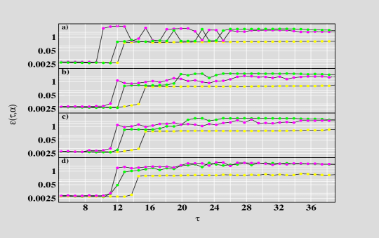
Figure 3: For $\alpha=1$ (yellow), $\alpha=5$ (green) and $\alpha=20$ (magenta) and $\omega_{\lambda}=0$, a) plot of $\epsilon$ vs $\tau$ for deterministic CCS trajectories ($\omega_{x}=0$). Similar plots for stochastic trajectories with b) $\omega_{x}=5$, c) $\omega_{x}=10$ and d) $\omega_{x}=25$. Parameter values, initial condition and numerical integration as in Fig.2. Here, each $\epsilon$ value has been computed for $1\times 10^{6}$ time steps.

II.1.2 CCS control efficiency

A meaningful way to characterize further the CCS dynamics is to quantify the control capacity to increase and mantain long-term explotation within a selected stable branch, as a function of the model paramaters. Accordingly, we quantify the efficiency as

$$\epsilon(\tau,\alpha)=\lim_{T\rightarrow\infty}\frac{\omega^{2}_{R}}{TM_{T}^{2}}\int_{0}^{T}\frac{\Phi(\tau,\alpha)H(\Phi(\tau,\alpha))H(-x(t))}{k_{\lambda}}dt$$ (6)

H denotes a Heavyside function, whose value is zero for negative argument or one otherwise. The product of the Heavyside functions in the integral plays the role of an AND boolean operator, entailing that the contributions to the time average of $\Phi$ are considered only if $\Phi$ is positive and $x$ negative. The variance of deviations from the initial to the final time T, in the denominator of (6), aims at amplifying differences between hysteretic (B2) and branch-confined (B3) control regimes. Without loss of generality, hereafter we set the reference value $\omega^{2}_{R}=1$ in (6).

In the next subsections we focus on the behavior of the efficiency as a function of the size of the observation window $\tau$, of the degree of control response $\alpha$ and of the variance of random fluctuations $\omega_{x}$ and $\omega_{\lambda}$.

II.1.3 Deterministic CCS efficiency

Figure 3a summarizes the behavior of the efficiency (6) over the deterministic CCS trajectories corresponding to different values in $\tau$ and $\alpha$. Efficient control rises sharply as the observation window is increased above an $\alpha$-specific threshold $\tau_{c}$ –since below this value the CCS undergoes exploitation runaway (B1). Above $\tau_{c}$, the behavior of the efficiency becomes highly dependent on the degree of control response. For a low control response $(\alpha=1)$, the efficiency exhibits a quasi-constant plateau for $\tau>\tau_{c}$. This plateau consists of hysteretic cases (B2). In cases of moderate ($\alpha=5$) and high ($\alpha=20$) degree of control response, the behavior of the CCS efficiency becomes non-trivial. For values $\tau\gg\tau_{c}$ the efficiency is remarkably enhanced (see the appearance of a second plateau occurring for $\tau\geq 25$ in Fig3a), as a result of the suppression of the CCS hysteretic control pathways, in favour of branch-confined recovery-exploitation cycles (B3). For intermediate values $\tau>\tau_{c}$, a combination of pathways (B2) and (B3) is observed –where low efficiency values correspond to hysteretic control pathways (B2). Such a $\tau$-dependent selection of control pathways is further illustrated by the histogram of the x variable in Fig.4a, for the high control response case. It shows that the dynamics of the CCS becomes confined to $\textit{x}<0$ values as $\tau$ is slightly shifted, which explains the alternace of low and high efficiency ranges appearing at intermediate $\tau$ values. Comparing the different control response cases in Fig.3a, it can be observed that the moderate one is the most efficient for $\tau\gg\tau_{c}$.

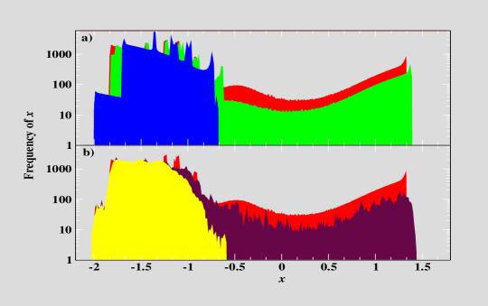
Figure 4: For $\alpha=20$, a) frequency histograms of CCS deterministic trajectories ($\omega_{x}=0$, $\omega_{\lambda}=0$) for $\tau=22.5$ (red), $\tau=22$ (green) and $\tau=19.5$ (blue). For $\tau=22.5$ and $\omega_{\lambda}=0$, b) histograms of stochastic trajectories with $\omega_{x}=10$ (brown) and $\omega_{x}=25$ (yellow), as well as histogram of the deterministic case (red), as in panel a). Parameter values, initial condition and numerical integration as in Fig.(2).

II.1.4 Stochastic CCS efficiency

Let us address now the case where the evolution of x is marked by continuous random perturbations (i.e., $\omega_{x}\neq 0$, $\omega_{\lambda}=0$ in Eqs. (1) and (2)). Panels b) to d) in Fig.(3) illustrate the influence of noise on the CCS efficiency. In the case of low control response, the behavior of the efficiency with $\tau$ appears to be independent of the standard deviation of noise $\omega_{x}$. In contrast, for moderate and high control responses, the overall efficiency becomes enhanced by an increase in the intensity of noise, in the sense that low efficiency values tend to disappear while high efficiency occurs all the way above the $\tau_{c}$-value (compare Fig.3a with Figs. 3b–d). However, if the variance of noise is marginally large (Fig.3a-c), the high control response case is less efficient as compared with the moderate one. For strong noise (Fig.3d), both moderate and high control response cases converge to a similar efficiency value for large $\tau$.

Since, for high and moderate response cases, low efficiency values tend to disappear when increasing intensity noise, it is natural to inquire about the influence of strong noise on hystheretic pathways. This effect is shown by the histogram of x Fig.4b for a single realization with $\alpha=20$. Notice the similarity between panels (a) and (b), which illustrates the equivalence in the control pathway selection that occurs either by changes in $\tau$ (Fig.4a) or by an increase in the standard deviation of the random fluctuations $\omega_{x}$ (Fig.4b).

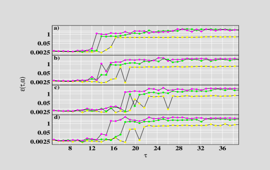
Figure 5: For $\alpha=1$ (yellow), $\alpha=5$ (green) $\alpha=20$ (magenta) and $\omega_{x}=0$, plot of $\epsilon$ vs $\tau$ for stochastic CCS trajectories with a) $\omega_{\lambda}=5$, b) $\omega_{\lambda}=10$ and c) $\omega_{\lambda}=20$. In d), similar plots for $\omega_{\lambda}=25$ and $\omega_{x}=20$. Parameter values, initial condition and numerical integration as in Fig.2. Here, each $\epsilon$ value has been computed for $1\times 10^{6}$ time steps.

Interestingly enough, we observe a similar effect of efficiency enhancement and uniformization in the case of noise at the level of the control system (i.e., $\omega_{x}=0$, $\omega_{\lambda}\neq 0$) Fig.5a-c, as compared with the deterministic CCS (Fig.3a). However, in this case the emergence of efficient control occurs for larger values in $\tau$, as the intensity of noise increases. Finally, in the case of strong noise at the level of both the state variable x and control (i.e., $\omega_{x}\gg 0$, $\omega_{\lambda}\gg 0$) Fig.5d, the case of high control response becomes the most efficient one, in comparison with the ($\omega_{x}\neq 0$, $\omega_{\lambda}=0$) cases (Fig.3d).

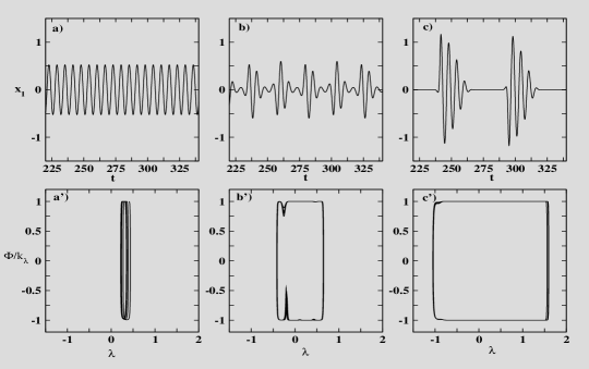
Figure 6: Behavior of the deterministic HCS ($\omega_{x}=0,\omega_{\lambda}=0$). Plot of $x_{1}$ vs time for a) $\tau=0.5$, b) $\tau=3$, c) $\tau=10$. Corresponding to these $\tau$ values, panels a’)-c’) show the plot $\Phi/k_{\lambda}$ vs $\lambda$.

II.2 The Hopf-control system (HCS)

A relevant and also frequently observed type of regime shift consists in the onset of time periodic behavior, as a stationary system regime becomes unstable at a threshold value in a system parameter. Examples of processes and systems where such phenomenon is present are for instance, chemical clocks at the mesoscopic McEwen and macroscopic Epstein scales, cellular biochemical cycles Goldbeter , prey-predator population dynamics Murray , shallow lake ecosystems Scheffer , the ocean-atmosphere system Vallis , or non-equilibrium economics models Hallegatte . All models accounting for the emergence of oscillatory behavior involve at least two variables and in all cases it has been possible to assimilate the mechanisms underlying the critical onset of oscillations to a Hopf bifurcation Guckenheimer . In what follows we focus on the dynamics of the coupled system of control (2)-(3) and the deterministic evolution law in (1), given by the Hopf normal form –which we refer hereafter as the Hopf-control system (HCS). For illustrative purposes and without loss of generality, we consider the supercritical version of the Hopf normal form

$$\begin{array}[]{c l}F_{1}(x_{1},x_{2},\lambda)=\lambda x_{1}-x_{2}-x_{1}(x_{1}^{2}+x_{2}^{2}),&F_{2}(x_{1},x_{2},\lambda)=\lambda x_{2}-x_{1}-x_{2}(x_{1}^{2}+x_{2}^{2})\end{array}$$ (7)

The stationary solution $x_{1}=0$, $x_{2}=0$ to the Hopf normal form (7) losses stability as $\lambda$ approaches zero along the negative axis. Above the critical value $\lambda_{c}=0$, the system variables $(x_{1},x_{2})$ describe stable oscillations whose amplitudes increase as $\sqrt{\lambda}$.

Here, the control functional (3) is fed by either of both system variables $(x_{1},x_{2})$, whose dynamics is subjected to stochastic perturbations with same standard deviation $\omega_{x}$.

II.2.1 Deterministic HCS dynamics

For an initial condition around the stationary solution $x_{1}=0$, $x_{2}=0$ and for an intial value $\lambda<0$, Figs.6a-c show the deterministic dynamics of the $x_{1}$ component under the influence of control for different values of the time window $\tau$. In complete absence of control, the linear growth in the value of $\lambda$, beyond the critical point, leads to oscillations of increasing amplitude $\sqrt{\lambda}$. In contrast, for small values $\tau\gtrsim 0$ the amplitude of oscillations becomes constant (Fig.6a). In this situation, both recovery ($\Phi<0$) and exploitation ($\Phi>0$) phases succeed each other rapidly, while the control variable always remains above the critical value $\lambda_{c}=0$ (Fig. 6a’). A further increase in $\tau$ induces a temporal alternance of small and large oscillation amplitudes (Fig.6b), as the recovery and exploitation phases lead the system back and forth accross $\lambda_{c}$ (Fig.6b’). If $\tau$ is large enough, oscillations are temporally suppressed (Fig.6c), during a time interval that increases with $\tau$. This situation results from the fact that the $\lambda$-interval covered by the recovery and exploitation phases becomes enlarged (Fig.6c’). In contrast with the CCS Fig.5c, no substantial increase in the complexity of the dynamics is observed as the time window $\tau$ is arbitrarily increased.

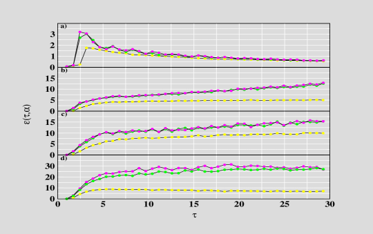
Figure 7: For $\alpha=1$ (yellow), $\alpha=5$ (green), $\alpha=20$ (magenta) and $\omega_{\lambda}=0$, a) plot of $\epsilon$ vs $\tau$ for deterministic HCS trajectories ($\omega_{x}=0$). Similar plots for stochastic trajectories with b) $\omega_{x}=5$, c) $\omega_{x}=10$ and d) $\omega_{x}=25$. Parameter values, initial condition and numerical integration as in Fig.2. Here, each $\epsilon$ value has been computed for $1\times 10^{6}$ time steps.

II.2.2 Deterministic and stochastic HCS efficiency

In a similar vein as for the CCS, we define the efficiency of the HCS as the capacity to increase and mantain long-term subcritical explotation, while keeping the oscillation amplitudes to a minimum. Thus we write the efficiency as

$$\epsilon(\tau,\alpha)=\lim_{T\rightarrow\infty}\frac{\omega^{2}_{R}}{TM_{T}^{2}}\int_{0}^{T}\frac{\Phi(\tau,\alpha)H(\Phi(\tau,\alpha))H(-\lambda(t))}{k_{\lambda}}dt$$ (8)

where H denotes a Heavyside function, such as defined for (6).
As shown by Figs.6a’–c’, subcritical exploitation increases with the size of the observation window $\tau$. However, it is also observed that the amplitude of oscillations along the recovery phase also increases with $\tau$ (Figs.6a–c). Therefore, an optimum is expected to occur in the efficiency (8) as a function of $\tau$. This situation is actually illustrated in Fig.7a for different degrees of control response. Notice that compared to the efficiency of the deterministic CCS Fig.6a, the sharp rise towards efficient control occurs at a small value $\tau_{c}$, above which efficiency gradually decays for larger $\tau$ values.

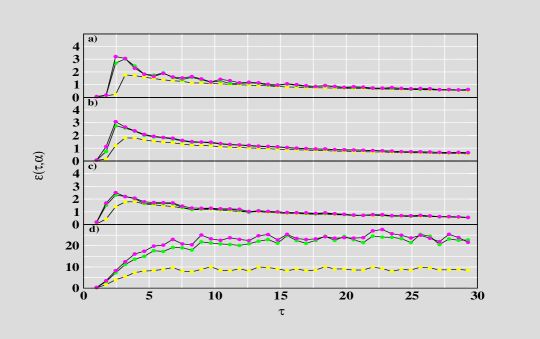
Figure 8: For $\alpha=1$ (yellow), $\alpha=5$ (green) $\alpha=20$ (magenta) and ($\omega_{x}=0$), plot of $\epsilon$ vs $\tau$ for stochastic HCS trajectories with a) $\omega_{\lambda}=5$, b) $\omega_{\lambda}=10$ and c) $\omega_{\lambda}=20$. In d), similar plots for $\omega_{\lambda}=25$ and $\omega_{x}=20$. Parameter values, initial condition and numerical integration as in Fig.2.

In presence of noise at the level of the system variables ($x_{1},x_{2}$) (i.e. $\omega_{x}\neq 0,\omega_{\lambda}=0$), it is observed that the efficiency increases along with $\tau$, for the moderate and high control response cases, while for low control response it remains at low practically constant value (Fig.7b). Similarly as for the CCS (Fig.3), the efficiency is in overall enhanced by the intensity of noise Fig.7b–d. Moreover, the behavior of the efficiency is practically the same for moderate and high control response cases, with the exception of the strong noise case Fig.7d, where high control response is highest for arbitrary large $\tau$ values.

When considering the effect of stochastic perturbations on the control dynamics (i.e. $\omega_{x}=0,\omega_{\lambda}\neq 0$) Figs.8a–c, the behavior of the efficiency remains qualitatively the same as in the purely deterministic case Fig.7a. Regardless the intensity of control fluctuations, a maximum in efficiency is observed at an approximately same $\tau$ value. The efficiency associated with high and moderate control responses exhibit a similar dependency on $\tau$. In both cases, the maximum in efficiency is higher as compared to the low response one. However, the highest efficiency peaks are slightly lowered when augmenting the intensity of noise at the level of control. For all the control response cases, when increasing $\tau$ the corresponding efficiencies tend to converge to a same low value, independently of the intensity of noise in control.

Finally, in presence of strong fluctuations at the level of the dynamics of both the system and the control (i.e. $\omega_{x}\gg 0,\omega_{\lambda}\gg 0$), the efficiency rises towards a plateau for larger values of $\tau$. In this case it is observed that the presence of strong fluctuations enhances the control efficiency and to a greater extent in the cases of high and moderate control response.

III Summary and conclusions

In this work we addressed the variance-based control of systems evolving towards criticality. As testbed models we considered the cusp and Hopf normal forms, displaying the prototypical phenomena of bistability and oscillations, respectively.

In relation to the core questions i)–iii) exposed in Sec. I, our main results can be summarized as follows:

i) In absence of noise, effective control in both the cusp and the Hopf systems rises above a threshold value in the size of the observation time window.

ii) In the cusp-control system, changes in the observation time window provide a means to selecting among different control pathways, namely, hysteretic, branch-confined control, as well as an intermittent combination of both. The branch-confined regime becomes dominant when considering a large observation window. This entails an increase in the complexity of the dynamics, in the form of aperiodic control-system trajectories. In the case of the Hopf-control system, the crossing of the bifurcation point could not be avoided, for the range of paramaters explored. Instead, as the observation time window is enlarged, exploitation and recovery phases occur for longer periods. This gives rise to the alternace of time intervals where oscillations are suppressed, followed by amplified oscillations.

iii) In both systems, random fluctuations, at the level of the system variables, enhance the efficiency of control, and especially for large observation time windows. In the case of the cusp-control system, the intensity of noise induces a control pathway selection, similarly as in the deterministic case when varying the observation time window. From the deterministic to the strong fluctuations cases, the efficiency of the cusp-control system tends to increase for large values in the size of the observation window. In the Hopf-control system, an increase in the intensity of noise induces a reduction in the amplitude of oscillations, which entails an increase in the control efficiency. Random fluctuations at the level of the control dynamics exert opposite influences on the control efficiency of the cusp and Hopf control systems. In the former it increases, while for the latter it tends to diminish the peak of efficiency. For both cusp and Hopf control systems, the combination of fluctuations in the control and in the system dynamics amplifies the efficiency in particular for large observation time windows. Regarding the interplay between the efficiency, the degree of control response, the intensity of noise, and the observation time window, we observe: in both systems, the low control response case exhibits a low efficiency, independently of the intensity of noise and observation window. When increasing the variance of fluctuations in the dynamics of the cusp system, a moderate control response leads to a higher efficiency; the opposite situation occurs when considering fluctuations on the control dynamics. In the Hopf system, the moderate and high control response perform very similar, regardless the intensity of noise and size of the time window. In this situation, for both moderate and high response cases, the efficiency converges to the lower value associated with a low control response, as the observation time window is increased.

For the systems here addressed, it remains to be studied the influence of other parameters, such as the rate of change in the control system ($k_{\lambda}$), the control reference parameter ($V_{R}$), as well as alternative approaches towards bifurcation, such as variation of the parameter $\mu$ in the cusp map –which would induce flickering patterns at the vicinity of the critical point.

Potential applications of this approach to real world systems include ecosystem models, non-equilibrium mesoscopic physico-chemical systems or non-equilibrium models in economics, among others. Similarly, it is of interest to extend this work to address the control properties associated to different alternative early warning indicators. Moreover, our analisis could be extended to address the control of coupled systems, forming networks whose nodes consist in dynamical systems subject to control.

Certainly, the structure of the evolution equations of real world models, involving a large number of parameters, lacks the degree of symmetry that confers to normal forms their characteristic simplicity. Moreover, not every dynamical system exhibiting a bifurcation belongs to a class of universality. It is thus important to address further the relation between the observation time scales leading to effective control and the geometrical properties, such as the curvature, of the system solution branches, while considering different early warning indicators.

IV Acknowledgements

We acknowledge the Federal Ministry of Education and Research (BMBF) through the program “Spitzenforschung und Innovation in den Neuen Länden” (contract “Potsdam Research Cluster for Georisk Analysis, Environmental Change and Sustainability” D.1.1) and the European Community’s Seventh Framework Programme under Grant Agreement No. 308497 (Project RAMSES) for financial support. A.G.C.R. acknowledges Christian Pape, Prof. Gregoire Nicolis and Doctors Elena Surovyatkina, Vasileos Basios and Flavio Pinto for fruitful discussions and for encouraging this work.

References

- [1] Nicolis G. and Prigogine I. Exploring Complexity: An Introduction. W. H. Freeman Press, 1989.
- [2] R. Badii and Politi A. Complexity: Hierarchical structures and scaling in physics. Cambridge Press, 1997.
- [3] H. E. Stanley. Introduction to Phase Transitions and Critical Phenomena. Oxford Press, 1987.
- [4] Nicolis G. and Prigogine I. Self-organization in Nonequilibrium Systems. John Wiley and Sons Inc., 1977.
- [5] Cross M. and Greenside H. Pattern Formation and Dynamics in Nonequilibrium Systems. Cambridge Press, 2009.
- [6] Scheffer M., Carpenter S., Foley J.A., Folke C., and Walker B. Catastrophic shifts in ecosystems. Nature, 413:591–596, 2001.
- [7] Scheffer M. Critical Transitions in Nature and Society. Princeton Press, 2009.
- [8] Castellano C., Fortunato S., and Loret V. Statistical physics of social dynamics. Rev. Mod. Phys., 81:591–646, 2009.
- [9] Lenton T. M., Held H., Kriegler E., Hall J. W., Lucht W., Rahmstorf S., and Schellnhuber H. J. Tipping elements in the earth’s climate system. Proc. Natl. Acad. Sci., 105:1786–1793, 2008.
- [10] Gardiner C. Stochastic Methods: A Handbook for the Natural and Social Sciences. Springer-Verlag, 2009.
- [11] Guckenheimer J. and Holmes P. Nonlinear Oscillations, Dynamical Systems, and Bifurcations of Vector Fields, Applied Mathematical Sciences 42. Springer-Verlag, 1983.
- [12] Scheffer M. et al et al. Early-warning signals for critical transitions. Nature, 461:53–59, 2009.
- [13] Scheffer M. et al et al. Anticipating critical transitions. Science, 338:344–348, 2012.
- [14] Carpenter S. R. & Brock W. A. Rising variance: a leading indicator of ecological transition. Ecology Letters, 9:311–318, 2006.
- [15] Guttal V. and Jayaprakash C. Changing skewness: an early warning signal of regime shifts in ecosystems. Ecology Letters, 11:450–460, 2008.
- [16] Biggs R., Carpenter S. R., and Brock W. A. Turning back from the brink: Detecting an impending regime shift in time to avert it. Proc. Nat. Acad. Sci. USA, 106:826–831, 2009.
- [17] Livina V.N. and Lenton T. M. A modified method for detecting incipient bifurcations in a dynamical system. Geophys. Res. Lett, 34:L03712, 2007.
- [18] Dakos V. et al et al. Methods for detecting early warnings of critical transitions in time series illustrated using simulated ecological data. PLoS ONE, 7:e41010, 2012.
- [19] Hilborn R. Reinterpreting the state of fisheries and their management. Ecosystems, 10:1362–1369, 2007.
- [20] Scheffer M., Hosper S. H., Meijer M. L., and B. Moss. Alternative equilibria in shallow lakes. Trends Ecol. Evol., 8:275–279, 1993.
- [21] Nicolis G. and Nicolis C. Dynamics of switching in nonlinear kinetics. J. Phys.: Condens. Matter, 19:065131, 2007.
- [22] Nicolis G. Introduction to Nonlinear Science. Cambridge Press, 1999.
- [23] V. Dakos, van Nes E.H., D’Odorico P., and Scheffer M. Tipping elements in the earth’s climate system. Ecology, 9:264–271, 2012.
- [24] Boettiger C. and Hastings A. Quantifying limits to detection of early warning for critical transitions. Interface, 9:2527–2539, 2012.
- [25] McEwen J.S., García Cantú Ros A., Gaspard P., Visart de Bocarme T., and Kruse N. Non-equilibrium surface pattern formation during catalytic reactions with nanoscale resolution: Investigations of the electric field influence. Catalysis Today, 154:75–78, 2010.
- [26] Epstein I.R. and Pojman J.A. An introduction to nonlinear chemical dynamics: oscillations, waves, patterns, and chaos. Oxford Press, 1998.
- [27] Goldbeter A. Biochemical Oscillations and Cellular Rhythms: The Molecular Bases of Periodic and Chaotic Behaviour. Cambridge Press, 1997.
- [28] Murray G.D. Mathematical Biology: I. An Introduction. Springer-Verlag, 2000.
- [29] Vallis G.K. Conceptual models of el niño and the southern oscillation. J. Geophys. Res., 93:13979–13991, 1988.
- [30] Hallegatte S., Ghil M., Dumas P., and Hourcade J.C. Business cycles, bifurcations and chaos in a neo-classical model with investment dynamics. Journal of Economic Behavior and Organization, 67:57–77, 2008.