Drag correlation for dilute and moderately dense fluid-particle systems using the lattice Boltzmann method

Abstract

This paper presents a numerical study of flow through static random assemblies of monodisperse, spherical particles. A lattice Boltzmann approach based on a two relaxation time collision operator is used to obtain reliable predictions of the particle drag by direct numerical simulation. From these predictions a closure law $F(Re_{p},\varphi)$ of the drag force relationship to the bed density $\varphi$ and the particle Reynolds number $Re_{p}$ is derived. The present study includes densities $\varphi$ ranging from $0.01$ to $0.35$ with $Re_{p}$ ranging up to $300$, that is compiled into a single drag correlation valid for the whole range. The corelation has a more compact expression compared to others previously reported in literature. At low particle densities, the new correlation is close to the widely-used Wen & Yu – correlation.

Recently, there has been reported a discrepancy between results obtained using different numerical methods, namely the comprehensive lattice Boltzmann study of Beetstra et al. (2007) and the predictions based on an immersed boundary - pseudo-spectral Navier-Stokes approach (Tenneti et al., 2011). The present study excludes significant finite resolution effects, which have been suspected to cause the reported deviations, but does not coincide exactly with either of the previous studies. This indicates the need for yet more accurate simulation methods in the future.

1 Introduction

Many of the mineral processing unit operations involve multi-phase systems that can be classified as either solid-liquid system such as hydrocyclone, high wet intensity magnetic separator, fluidized bed, thickener, spiral concentrator; solid-gas system such as gas fluidized bed; or solid-gas-liquid system such as flotation column. The volume fraction of solid particles that is fed into these units varies from sometimes very low concentrations as in the case of hydrocyclones or magnetic separators to very high concentrations as in the case of fluidized beds. The mineral processing industry is considered as one of the most polluting industries and therefore it is desirable to use only as few experiments as possible. Computer simulations prior to and accompanying experiments cannot only reduce the number of experiments, but are also cheaper. With the advent of high speed computers, it is now possible to obtain solutions faster and with better accuracy. This does not only save time, money and material, but is also pollution-free.

Several approaches like continuum models (Swain and Mohanty, 2013; Mohanty et al., 2011), discrete models (Mishra and Tripathy, 2010) and a combination of discrete and continuum models (Chu et al., 2009) have been reported in literature for various mineral processing unit operations. In practice, multi-fluid models such as Eulerian-Eulerian models, which treat the phases as inter-penetrating continua, are more common because in an actual system it is difficult to capture the dynamics of all individual particles present. It has been reported by van der Hoef et al. (2006) that for millimeter size particles the linear dimension of the system that can be simulated with the existing computers is about $0.1$ m. For larger systems, multi-fluid continuum models have become more popular that treat the granular solid phase as a continuum and the momentum balance equations for both the phases are solved to predict the flow profile of the phases. These mathematical models require several closure laws, primarily for the drag force, to account for the momentum exchange between the phases. The earliest correlations available were those by Wen and Yu (1966) for dilute systems and the Ergun’s equation (Ergun, 1952) for denser systems. Both are based on experimental data. Other correlations commonly used in two-fluid models are the ones proposed by Gidaspow (1986) and Shyamlal and O’Brien (1987). The Gidaspow correlation reduces to the Wen and Yu correlation for low solid volume fraction and Ergun’s equation at high solid volume fraction. The correlation by Shyamlal and O’Brien is based on the terminal velocity correlation proposed by Richardson and Zaki (1954). The reliability of these correlations for mono-dispersed system has been questioned by some authors (Beetstra et al., 2007), as Ergun derived the correlation based on experiments carried out using sand and pulverized coke in addition to that carried out with spheres.

1.1 Studies on drag closure laws based on DNS

With the advent of high speed computers, several direct numerical simulation (DNS) methods have been adopted by a number of researchers to obtain drag closure laws. Pioneering studies on particulate suspensions by Ladd (1994a, b); Ladd and Verberg (2001) using the lattice Boltzmann method (LBM) enabled the work on establishing drag closure laws. The earliest systematic studies on drag force relations by Hill et al. (2001a) considered a fixed bed of spheres arranged in simple cubic, face centered and random order. The volume fraction of solids ranged from approximately $0.001$ to $0.64$ at low Reynolds number $Re_{p}$. Subsequently, the effect of the Reynolds number, up to $Re_{p}\leq 100$, on the drag force for the same arrangement of spheres was studied by the same authors (Hill et al., 2001b). Later, van der Hoef et al. (2005) used LBM to study the drag force on fixed arrays of mono-dispersed and bi-dispersed spheres arranged in random order in the limit of zero Reynolds number. They established a normalized drag force correlation, defined as the ratio of the drag force for a given Reynolds number and solid volume fraction to that calculated using the Stokes-Einstein equation. They also reported that when their drag force correlation was extrapolated to $Re_{p}=0$, there was no significant difference between drag force at $Re_{p}=0.2$ and $Re_{p}=0$. Beetstra et al. (2007) later extended this work to $Re_{p}$ up to $1000$. They also obtained a correlation for the normalized drag force as a function of solid volume fraction and Reynolds number. Reportedly, the Ergun type correlation fits the simulation data better than the Wen and Yu type. Benyahia et al. (2006) modified the correlations proposed by Hill et al. (2001a) so that a continuous function can be obtained for all range of solid volume fraction and Reynolds number. Tenneti et al. (2011) have used a particle resolved DNS method that they call “Particle-resolved Uncontaminated-fluid Reconcilable Immersed Boundary Method” to study the drag force on a fixed array of randomly arranged assembly of mono-dispersed spheres in the solid volume fraction range of 0.1-0.4 and Reynolds number up to 300. The results are compared with Hill et al. (2001b) and Beetstra et al. (2007). The three studies agree quite well at low Reynolds number. At higher Reynolds number, the data of Tenneti et al. (2011) and Beetstra et al. (2007) disagree by up to $30\%$. Tenneti et al. (2011) attribute the mismatch to the constant resolution used in Beetstra et al. (2007) over the whole range of Reynolds numbers.

All of the above studies assume static beds of spheres without changes in the relative positions. However, some work on moving particles for bi-dispersed spheres of equal size but different densities (Yin and Sundaresan, 2009a) as well as of different sizes (Yin and Sundaresan, 2009b) at low Reynolds number and solid volume fraction of $0.1..0.4$, have been reported using LBM. Holloway et al. (2010) used the data from Yin and Sundaresan (2009a, b) and that by Beetstra et al. (2007) to obtain a drag correlation for poly-dispersed particles in the solid volume fraction range $0.2..0.4$, particle diameter ratio between $1$ and $2.5$ and $0\leq Re_{p}\leq 40$.

1.2 Objective of the present study

Most studies using LBM have reported drag laws for solid volume fraction above $0.1$ and higher Reynolds numbers, primarily aimed at fluidized beds. Hence, there is currently a lack of studies carried out in the low solid volume fraction range, except for the results reported by Hill et al. (2001b) for low Reynolds numbers. Several unit operations in mineral processing operate with lower solid volume fractions and higher Reynolds number. Also, in the same system there can be regions with low as well as high solid volume fraction. Therefore a drag law applicable over a wider range of particle concentration, including solid volume fraction $\leq 0.1$ at a given range of Reynolds number would be desirable. In the following study, a drag law for solid-fluid dispersions with solid volume fraction ranging from $0.01$ to $0.35$ and Reynolds numbers $Re_{p}\leq 300$ is derived from simulations.

All the lattice Boltzmann studies on fluid-particle drag mentioned in Sec. 1.1 have been carried out with the code developed by Ladd (Ladd, 1994a, b; Ladd and Verberg, 2001). One common disadvantage of these efforts is that the sphere is represented by a staircase like approximation (bounce back boundary conditions) in simulations and thus a certain error will be introduced. However, it has been established already in the original work that LBM still delivers accurate predictions, for instance by comparing it with analytical solutions for Stokes flow of Hasimoto (1959) and Sangani and Acrivos (1982). Another common disadvantage of the aforementioned LBM studies is the usage of a single relaxation time collision operator. This is known to introduce a viscosity-dependent error in the boundary placement (Ginzbourg and Adler, 1994), and forces the authors to apply a correction for the effective hydrodynamic radius of the particles for the given relaxation time. The present work is based on a two relaxation time lattice Boltzmann code, tailored to circumvent the viscosity-dependent boundary placement (Ginzbourg and Adler, 1994; Ginzburg et al., 2008) to obtain more reliable results. Details on the simulation methodology are given in Sec. 2. Simulation results can be found in Sec. 3. The presentation of the main results of this paper in Sec. 3.3 - 3.5 is preceeded by a verification experiment of the numerical model (Sec. 3.1). Most importantly, we have conducted a resolution sensitivity study to show that there is no significant error stemming from under-resolved physics in the present study (Sec. 3.2).

Without relying on supercomputers the present study would not have been successful, as simulation of dilute particle concentrations at high Reynolds numbers is quite resource demanding. E.g., for $\varphi=0.01$ at a resolution of $d=40$ lattice sites per particle diameter, one needs a domain size of approximately $450^{3}$ grid points. To accomplish efficient simulations, the present study is based on the waLBerla code base (Feichtinger et al., 2011). This framework has been shown to offer extendibility to numerous physical applications involving fluid-structure interaction (e.g., Bogner and Rüde, 2013), while providing a highly efficient implementation for a wide range of supercomputers, even for complex fluids like suspensions (Götz et al., 2010).

2 Numerical Method: Two Relaxation Time LBM for Particle Beds

For the simulated hydrodynamics we employ a lattice Boltzmann approach (Benzi et al., 1992; Chen and Doolen, 1998; Aidun and Clausen, 2010) using the D3Q19 lattice model (Qian et al., 1992). The evolution of the distribution function $\mathbf{f}=(f_{0},f_{1},..,f_{Q-1})$ on the lattice for the finite set of lattice velocities $\{\mathbf{c}_{q}\,|\,q=0,..,Q-1\}$ is described by the following equations, Eq.s (1) and (2). We use a collision operator with two relaxation times as proposed by Ginzburg et al. (2008); Ginzburg (2005).

$$f_{q}(\mathbf{x}+\mathbf{c}_{q},t+1)=\tilde{f_{q}}(\mathbf{x},t),\\$$ (1)

$$\tilde{f_{q}}(\mathbf{x},t)=f_{q}(\mathbf{x},t)+\lambda_{+}(f_{q}^{+}-f_{q}^{eq,+})+\lambda_{-}(f_{q}^{-}-f_{q}^{eq,-})+F_{q},$$ (2)

Here, Eq. (1) is referred to as the streaming step, and Eq. (2) is the collision step, with independent relaxation times $\lambda_{+},\lambda_{-}\in(-2,0)$ for the even (symmetric) and odd (anti-symmetric) parts of the distribution function. Often the symmetric relaxation time is expressed as $\tau=-1/\lambda_{+}\in(0.5,\infty)$. $F_{q}$ is a source term that will be defined later. For the discrete range of values $q\in\{0,..,Q-1\}$, the opposite index $\bar{q}$ is defined by the equation $\mathbf{c}_{q}=-\mathbf{c}_{\bar{q}}$ and thus,

$$f_{q}^{+}=\frac{1}{2}(f_{q}+f_{\bar{q}}),\;\text{ and }\;f_{q}^{-}=\frac{1}{2}(f_{q}-f_{\bar{q}}),$$ (3)

respectively. The polynomial equilibrium function $\mathbf{f}^{eq}$ is given by

$$f_{q}^{eq}(\rho,\mathbf{U})=\rho w_{q}\left[1+\frac{\mathbf{c}_{q}^{T}\mathbf{U}}{c_{s}^{2}}+\frac{(\mathbf{c}_{q}^{T}\mathbf{U})^{2}}{2c_{s}^{4}}-\frac{\mathbf{U}^{T}\mathbf{U}}{2c_{s}^{2}}\right],$$ (4)

where the $w_{q}=w_{|\mathbf{c}_{q}|}$ are the lattice weights given in Qian et al. (1992), and $c_{s}=1/\sqrt{3}$ is the lattice speed of sound of the model. To exert a body force on the flow we use the source term

$$F_{q}=w_{q}\rho\left(\frac{\mathbf{c}_{q}-\mathbf{U}}{c_{s}^{2}}+\frac{\mathbf{c}_{q}^{T}\mathbf{U}}{2c_{s}^{4}}\mathbf{c}_{q}\right)^{T}\mathbf{a},$$ (5)

where $\mathbf{a}$ is a gravitation vector (Luo, 1998; Guo et al., 2002). Macroscopic quantities are defined as moments over $\mathbf{f}$. In particular, the moments of zeroth and first order,

$$\rho=\frac{1}{c_{s}^{2}}P =\sum_{q}f_{q},$$ (6)

$$\rho\mathbf{U}=\rho\mathbf{u}-\frac{\rho\mathbf{a}}{2} =\sum_{q}\mathbf{c}_{q}f_{q},$$ (7)

yield the pressure $P$ and fluid velocity $\mathbf{u}$. The shift in the fluid momentum by $\rho\mathbf{a}/{2}$ is necessary if a source term $F_{q}$ is used in Eq. (2) (cf. Buick and Greated, 2000; Ginzburg et al., 2008). The parameterization of $f^{eq}$ in Eq. (2) stays unchanged and is given by $f^{eq}_{q}=f^{eq}_{q}(\rho,\mathbf{U})$.

Fluid-structure interaction

To incorporate spherical particles into the flow, we use the bounce-back rule similar to Ladd (1994a, b), for all lattice links intersecting with the surface of a particle. For a boundary node $\mathbf{x}_{b}$ with boundary-intersecting link $q$ one has

$$f_{\bar{q}}(\mathbf{x}_{b},t+1)=\tilde{f_{q}}(\mathbf{x}_{b},t).$$ (8)

This approximation of a non-slip boundary condition can be made effectively independent of the lattice viscosity, $\eta=-(\lambda_{+}^{-1}+1/2)/3=(\tau-1/2)/3$ by fixing the second relaxation time $\lambda_{-}$, to satisfy

$$\Lambda_{\pm}:=(\frac{1}{2}+\frac{1}{\lambda_{+}})(\frac{1}{2}+\frac{1}{\lambda_{-}})\approx\frac{1}{4},$$ (9)

as shown by Ginzbourg and Adler (1994); Ginzburg et al. (2008); d’Humieres and Ginzburg (2009). The optimal value of $\lambda_{-}$ may slightly differ depending on the geometry of the flow (Ginzburg et al., 2008). Here, we used $\Lambda_{\pm}=3/16$. This is an important difference of the present approach from previous lattice Boltzmann studies on drag relations such as those reported by van der Hoef et al. (2005), Beetstra et al. (2007) and Hill et al. (2001a, b). These studies are all based on collision schemes that do not allow viscosity-independent simulations of flow around particles and thus come with an additional source of error, which can be controlled only by fixing the lattice viscosity to a constant value. Pan et al. (2006) have shown that the elimination of the viscosity-dependent error is significant, especially when relaxation times $\tau>1.0$ are used, as typically the case for low Reynolds-number flows. It should be noted, that the bounce-back rule yields a first-order accurate approximation of the particle boundaries (Ginzburg et al., 2008; Junk and Yang, 2005). Higher-order schemes (Bouzidi et al., 2001; Ginzburg and d’Humieres, 2003; Mei et al., 2002) exist, but are more complex to apply since they require interpolations over a number of compute nodes. Also, according to (Ginzburg et al., 2008; d’Humieres and Ginzburg, 2009; Pan et al., 2006), not all of them allow viscosity-independent parameterization according to Eq. (9), and thus may complicate the parameterization in terms of lattice viscosity. Hence, for the present study, we decided to use only the bounce-back rule, but to include a resolution sensitivity study, showing that the error due to boundary conditions is sufficiently converged (cf. Sec. 3.2).

The drag force exerted by the fluid on the particles is obtained by the momentum exchange algorithm (Ladd, 1994a; Yu et al., 2003). For a particle $p$, let $B_{p}$ be the set of boundary nodes, where for all $\mathbf{x_{b}}\in B_{p}$, the set of links $I_{p}(\mathbf{x_{b}})\subseteq\{0,..,Q-1\}$, intersecting with the surface of the particle $p$ is non-empty. The net force $\mathbf{f}_{p}$ exerted on the particle is then given by

$$\mathbf{f}_{p}=\sum_{\mathbf{x}_{b}\in B_{p}}\sum_{q\in I_{p}(\mathbf{x}_{p})}\Delta\mathbf{j}_{q}(\mathbf{x}_{b}),$$ (10)

where $\Delta\mathbf{j}_{q}(\mathbf{x}_{b})=\mathbf{c}_{q}(\tilde{f}_{q}+f_{\bar{q}})$ is the momentum transferred along a single intersecting link in direction $q$ from the boundary node $\mathbf{x}_{b}$. Note that in our specific case, the incoming population $f_{\bar{q}}$ is actually equal to the outgoing $\tilde{f}_{q}$ because of the bounce-back rule.

Drag force computations

The flow through random fixed configurations (beds) of $N$ non-overlapping spherical particles of diameter $d$ is simulated by accelerating the flow along a certain direction with a given uniform gravity $g$. The drag force evaluation is done after the flow has reached a balanced state. The particle Reynolds number is expressed as,

$$Re_{p}=\frac{\rho\bar{u}d}{\eta},$$ (11)

where

$$\bar{u}=\frac{\mathbf{a}^{T}}{|\mathbf{a}|L^{3}}\sum_{\mathbf{x}\in\Omega}(\mathbf{u}(\mathbf{x})-\mathbf{u}_{p})$$ (12)

is the average flow rate (directed with gravity $\mathbf{a}$) within a periodic cubic domain $\Omega$ of length $L$, relative to the particle velocity $\mathbf{u}_{p}$, that is taken as zero, since the particle positions are fixed with respect to the given frame of reference. The characteristic length $d$ can also be interpreted as the Sauter mean diameter that is often used to study heterogeneous, non-spherical particle beds. The approximated drag force $\mathbf{f}_{d}$ is obtained by averaging Eq. (10) over the whole number of particles, i.e., $\mathbf{f}_{d}=\frac{1}{N}\sum_{p=1}^{N}\mathbf{f}_{p}$. The solid volume fraction of the bed is given by

$$\varphi=\frac{NV_{p}}{V},$$ (13)

where $V_{p}$ is the particle volume, and $V=L^{3}$ the total volume of the bed.

In many practically relevant conditions, the flow in the particle bed will be driven by a static pressure gradient, yielding an additional buoyancy force $\mathbf{f}_{b}=-V_{p}\nabla P$ on each particle. Hence, the total hydrodynamic force (averaged per particle) is actually $\mathbf{f}_{t}=\mathbf{f}_{d}+\mathbf{f}_{b}$. Often, $\mathbf{f}_{t}$ is referred to as the drag force in literature. However, assuming the system to be in a balanced state, i.e., the driving force equals the total force exerted on the particles ($-V\nabla P=N\mathbf{f}_{t}$), the two definitions of the drag force can be directly related as $\mathbf{f}_{d}=(1-\varphi)\mathbf{f}_{t}$. Since a pressure gradient cannot be included in simulations using periodic domains, we will simply assume $\mathbf{f}_{b}=V_{p}\rho\mathbf{a}$ and interpret the results as equivalent to a pressure driven flow. The dimensionless drag force is accordingly defined as

$$C=\frac{f_{t}}{3\pi\eta d\bar{u}},\text{ or }C_{d}=\frac{f_{d}}{3\pi\eta d\bar{u}},$$ (14)

respectively.

3 Results: Simulation of Flow in Random Particle Beds

After two verification studies in Sec. 3.1 and Sec. 3.2, demonstrating the validity of our method, we study the flow through randomly generated fixed arrangements of spheres. Sec. 3.3 presents qualitative results for the most extreme cases studied. Finally, we present a comprehensive and systematic flow study in Sec. 3.4 including its compilation into a drag force closure relation and compare the result with two other numerical studies in Sec. 3.5. Quantities obtained as results from numerical experiments will be labeled with a superscript $*$ in the following.

3.1 Verification: Stokes flow in regular simple cubic array

For the verification of our code, we first evaluate the linear flow through a regular periodic array of spheres. For the case of a simple cubic array, Sangani and Acrivos (1982) have presented analytical results valid over a wide range of solid volume fractions $\varphi(\chi)=\pi\chi^{3}/6$, extending the prior work of Hasimoto (1959). By varying the radius $R$ of a sphere placed within a periodic unit cell of length $L=32$ and $L=64$ in lattice units, respectively, a set of different $\varphi$ is realized. The normalized drag force obtained from simulations, $C^{*}$, and the error relative to the analytical solution $C$ by Sangani and Acrivos (1982) is shown in Tab. 1. The average flow rate $\bar{u}^{*}$ in these simulations is also shown. Note, that the Mach and Reynolds numbers are always kept low (i.e., $u/c_{s}<0.01$ and $Re_{p}<0.03$) for exclusion of compressibility effects and assuring a good approximation to the Stokes regime, respectively. To speed up the convergence, the Mach number could be increased (typically one chooses $0.01<u/c_{s}<0.1$ (Succi, 2001) - here it was easier to compute with constant $\lambda_{+}=-1/3$ and gravitation $10^{-6}$). The relative errors are below $5\%$ in all cases, which shows the validity of our code. It also shows that the method is capable of accurate predictions of the drag force on spheres, even if the resolution of the sphere, or the gap in between the spheres, respectively, is relatively small.

Drag Force Computation in Simple Cubic Array
	$\varphi$	0.0042	0.014	0.034	0.065	0.11	0.18	0.27	0.38
$L$	$\chi$	0.2	0.3	0.4	0.5	0.6	0.7	0.8	0.9
$32$	R	3.2	4.8	6.4	8	9.6	11.2	12.8	14.4
	$\bar{u}^{*}$	4.75E-4	2.49E-4	1.51E-4	8.91E-5	5.45E-5	3.03E-5	1.59E-5	7.21E-6
	$C^{*}$	1.37	1.75	2.16	2.93	4.00	6.15	10.29	20.06
	$\frac{C^{*}-C}{C}$	-1.13%	2.74%	0.45%	2.93%	0.57%	2.49%	2.43%	4.69%
$64$	R	6.4	9.6	12.8	16	19.2	22.4	25.6	28.8
	$\bar{u}^{*}$	1.87E-3	1.02E-3	6.00E-4	3.61E-4	2.17E-4	1.23E-4	6.36E-5	2.97E-5
	$C^{*}$	1.39	1.70	2.17	2.89	4.00	6.08	10.25	19.52
	$\frac{C^{*}-C}{C}$	0.37%	0.27%	0.92%	1.63%	0.73%	1.27%	1.95%	1.86%

Table 1: Drag force on spheres in simple cubic array and the relative error compared to the analytic solution from Sangani and Acrivos (1982) at two different resolutions.

3.2 Verification: Resolution sensitivity

(a) $Re_{p}=100$
$\delta_{x}$	$\tau$	$d/\delta_{x}$	$Re_{p}^{*}$	$C_{d}^{*}$	$\delta_{b}/\delta_{x}$
0.02 (!)	0.500563	14.5726	102	26.6	1.4572
0.015625	0.500922	18.653	100	27.2	1.8653
0.01	0.50225	27.5089	99	27.5	2.751
0.005	0.509	58.2906	100	27.2	5.8291
(b) $Re_{p}=200$
$\delta_{x}$	$\tau$	$d/\delta_{x}$	$Re_{p}^{*}$	$C_{d}^{*}$	$\delta_{b}/\delta_{x}$
0.015625 (!)	0.500922	18.653	202	38.5	1.319
0.01	0.50225	29.1453	198	41.3	2.0609
0.005	0.509	58.2906	198	41.5	4.1218
0.0025	0.536	116.581	202	40.5	8.2435
(c) $Re_{p}=300$
$\delta_{x}$	$\tau$	$d/\delta_{x}$	$Re_{p}^{*}$	$C_{d}^{*}$	$\delta_{b}/\delta_{x}$
0.00625	0.50576	46.6325	300	55.4	2.6923
0.005	0.509	58.2906	300	55.6	3.3654
0.0025	0.536	116.581	300	54.0	6.7308

Table 2: Sensitivity of drag coefficient on resolution. The cases marked with (!) would eventually become unstable. Also shown is the approximate boundary layer thickness $\delta_{b}$ in lattice units.

		$d/\delta_{x}$
		46.6325	58.2906	116.581
$\Lambda_{\pm}$	3/16	55.4	55.6	54.0
	1/4	55.0	54.0	53.5
	3/8	53.4 (!)	54.0	53.4

Table 3: Normalized drag $C_{d}^{*}$ for various “magic parameter” settings in the $Re_{p}=300$ – case (c).

For particle Reynolds numbers in the unsteady regime numerical instabilities may arise in under-resolved cases. We therefore study the dependency of the estimated drag $C_{d}^{*}$ obtained from simulations on the grid spacing $\delta_{x}$. Our setup consists of a randomly arranged bed of $N=27$ spheres in a cubic periodic domain of unit length and solid volume fraction $\varphi=0.35$. In order to keep the Reynolds number constant while varying the resolution parameter $\delta_{x}$, we adjust the sphere diameter and lattice relaxation time accordingly (i.e., the apparent physical viscosity and length is kept constant). The study is repeated for three different target Reynolds numbers $Re_{p}=100$, $200$ and $300$.

For the first two cases ($Re_{p}=100$, $200$), the flow is driven by a constant body force starting from zero uniform initial velocity, and evaluated after a balanced state is reached. Tab. 2 shows the results for different Reynolds numbers. Due to the “staircase” discretization of the spheres the resulting $Re_{p}^{*}$ varies slightly. For the highest Reynolds number, $Re_{p}=300$, we dynamically adjusted the fluid acceleration $\mathbf{a}$ during simulations, in order to circumvent a manual calibration process. Even in the under-resolved situations marked with an (!) where one would expect instability, we observe that the predicted $C_{d}^{*}$-value does not deviate significantly from the well-resolved cases. From the magnitude of the deviations in the data (less than $3\%$ when excluding the unstable solutions), it can be concluded that the chosen lattice resolutions are sufficiently high. In fact, the results show that there is a minimum required resolution that increases with the Reynolds number, but also that further increase of resolution does not significantly effect the resulting drag forces. This is an important observation, since it has been reported by Tenneti et al. (2011) that previous studies based on the LBM (Beetstra et al., 2007) would lack validity at intermediate Reynolds numbers due to poor lattice resolutions. As noted by Tenneti et al. (2011), the boundary layer thickness ($\delta_{b}\sim d/\sqrt{Re_{p}}$) must be sufficiently resolved and can be used as a guideline when choosing the spatial resolution. For the given regime, one should have $\delta_{b}\sim 3$ or higher for numeric stability. Further increase of resolution yields only slight improvement in terms of accuracy. Hence for the following study in Sec.s 3.3-3.4, we chose grid spacings of the order of the second-to-last row of Tab. 2 as a compromise between accuracy and efficiency.

Influence of parameterization $\Lambda_{\pm}$ on numerical solution

For completeness, we also studied the influence of the magic parameter $\Lambda_{\pm}$ on the simulations in the transitional regime $Re_{p}=300$. This allows us to estimate the errors stemming from the parameterization of our scheme in Sec. 3.5, when comparing to the results from other authors – and the variation between the respective studies is most considerable for large $Re_{p}$. The optimal choice of $\Lambda_{\pm}$ is unknown for arbitrary geometries, so it is important to control whether the computed solutions depend on it. Because, for this regime, one has only small values of $\tau$, the effect on the solution is expected to be non-significant (cf. also Pan et al. (2006)). In Tab. 3 the resulting drags for different parameterizations is shown. Indeed, the influence was very small for the given geometry at the given relaxation times $\tau$. The parameterization $\Lambda_{\pm}=3/8$ lead to instabilities at the lowest resolution.

3.3 Study: Qualitative evaluation of different flow regimes

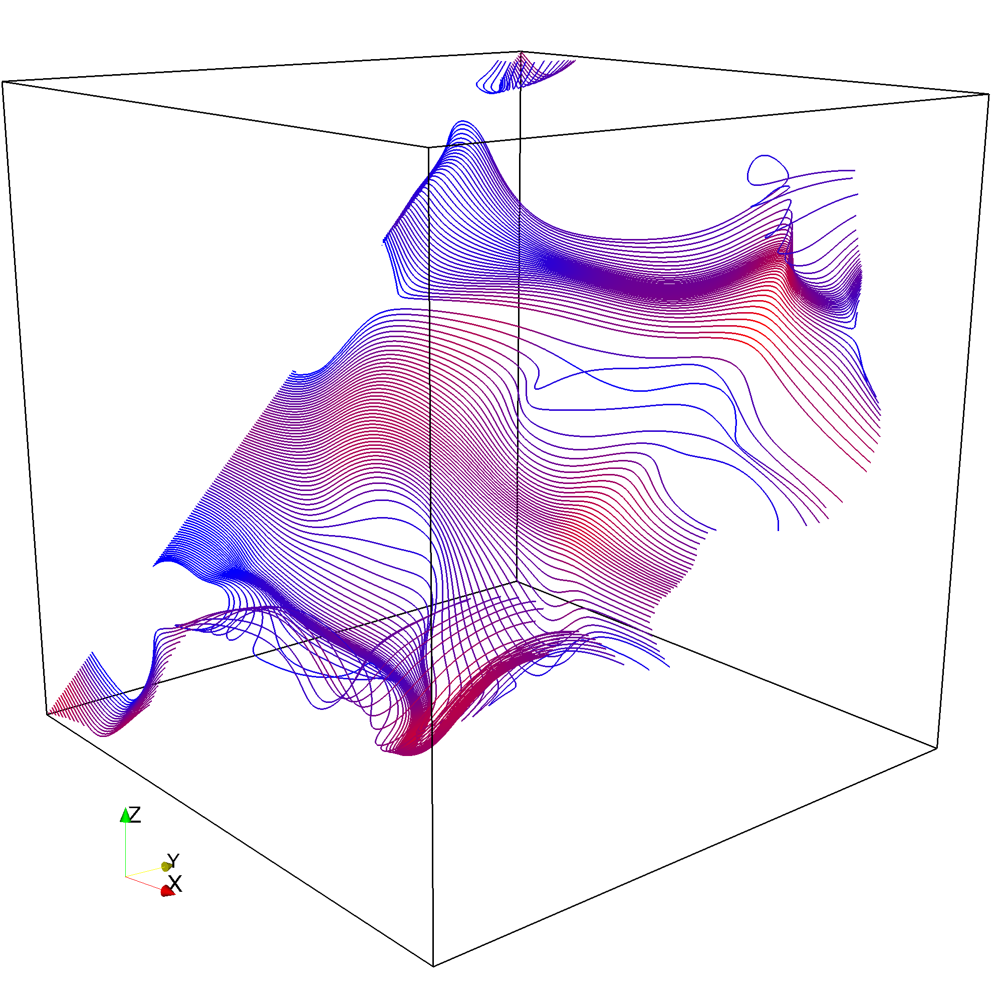
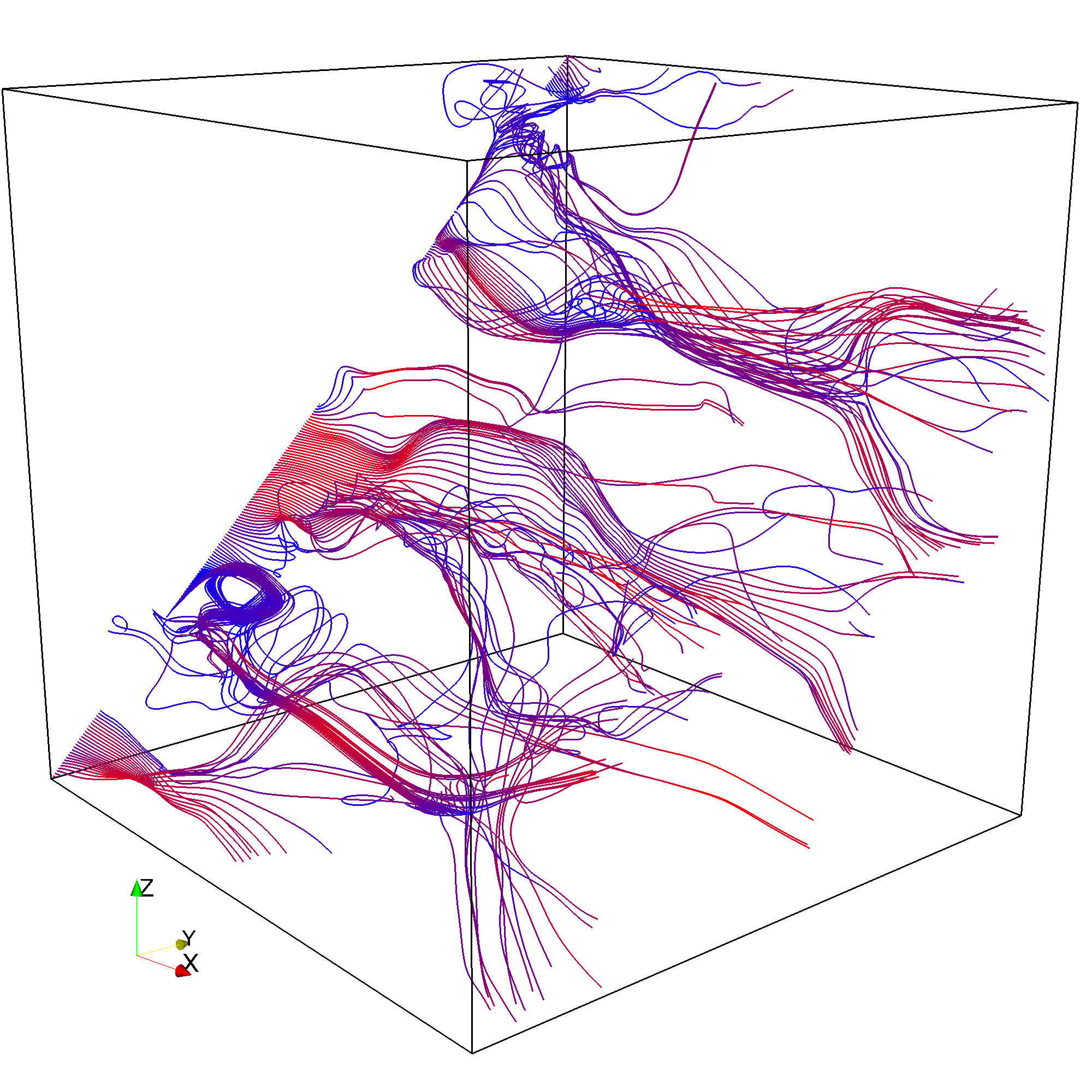
Figure 1: Streamlines in bed of solid volume fraction $\varphi=0.35$ in the laminar ($Re_{p}=3.6$, left), and in the transient regime ($Re_{p}=300$, right). Blue color indicates lower, red color indicates a higher flow velocity, respectively.

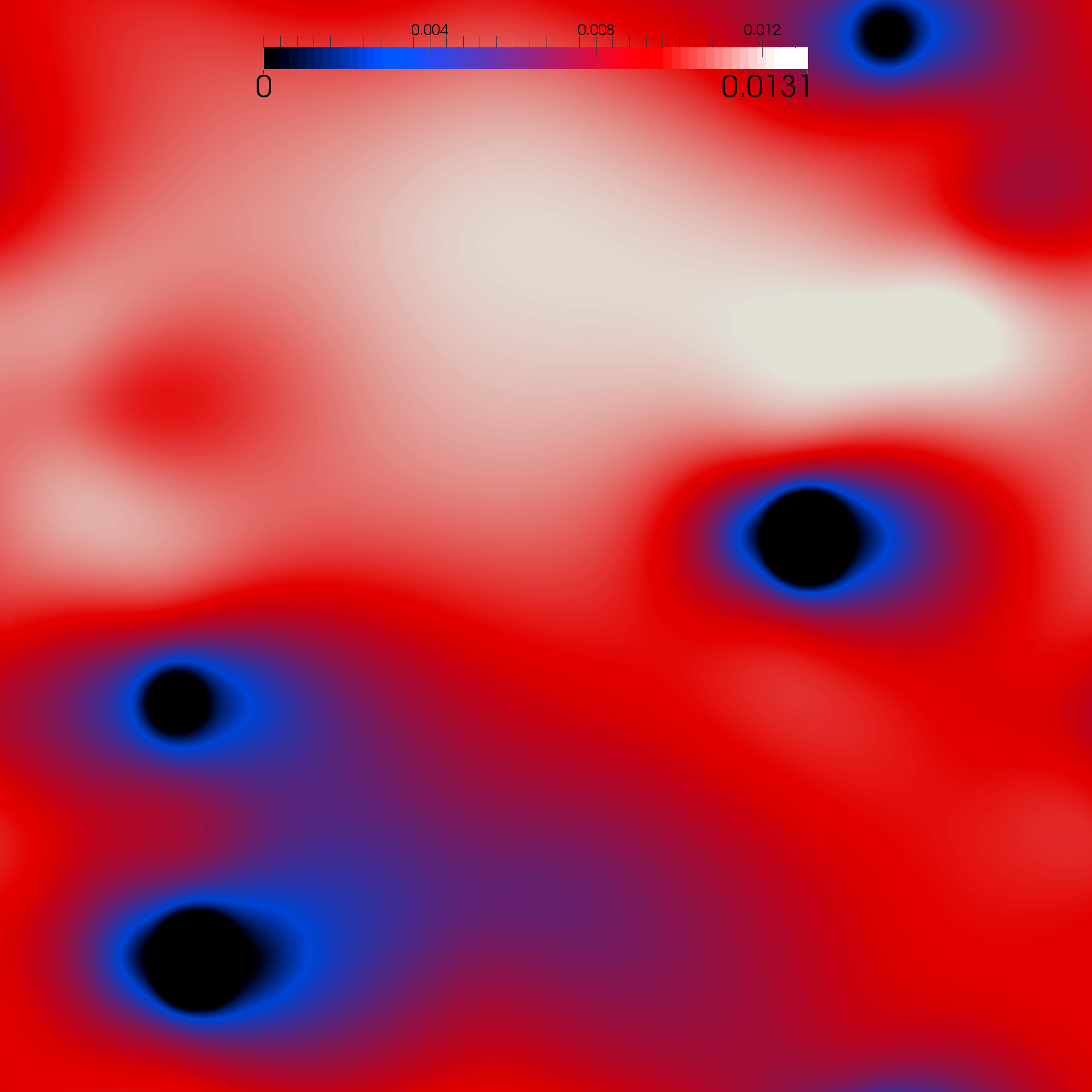
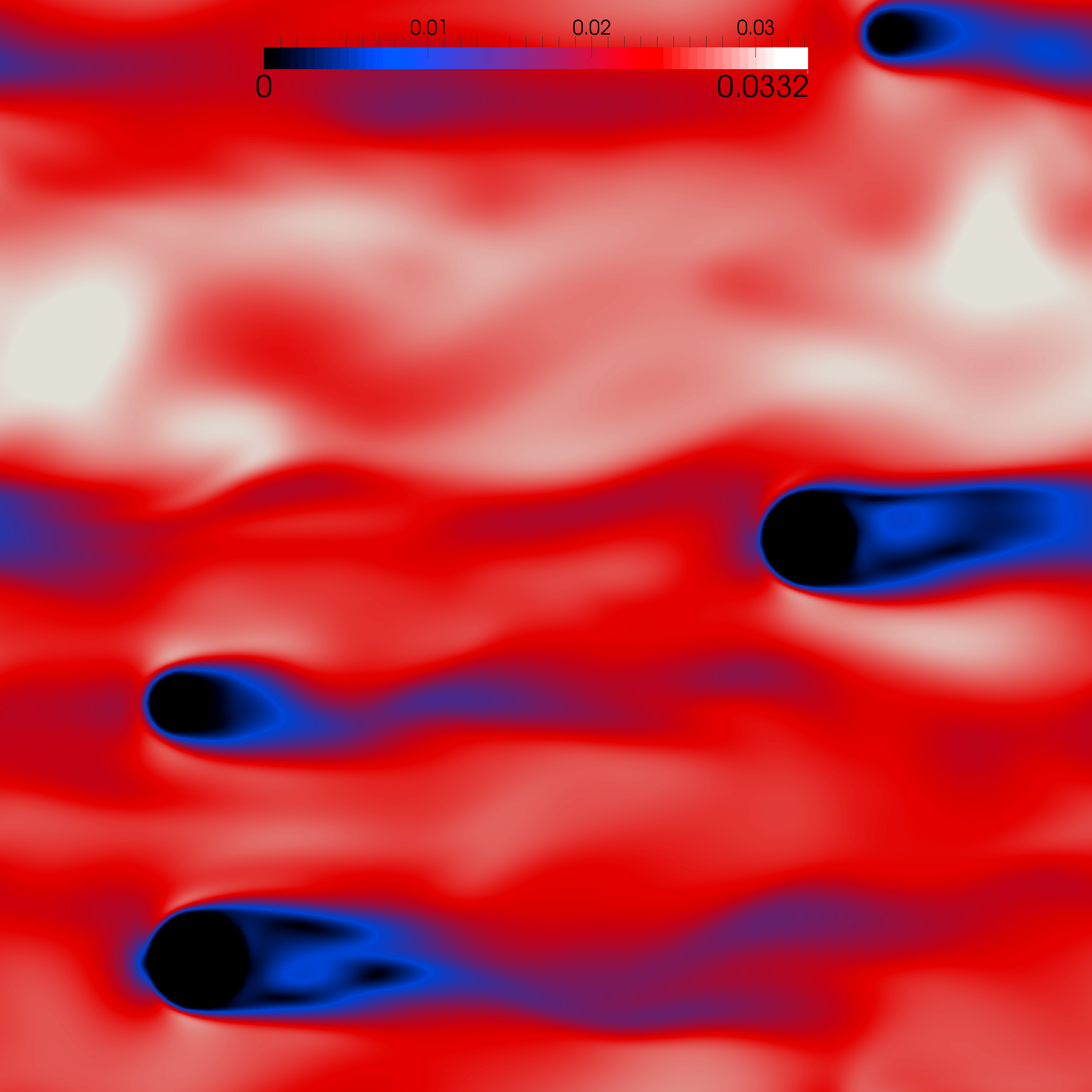
Figure 2: Velocity magnitude plot (slice $y=50$) in particle bed of volume fraction $\varphi=0.01$ in the laminar regime ($Re_{p}=2.4$, left), and in the transient regime ($Re_{p}=300$, right). Flow direction is from left two right in both cases. As indicated by the color bar, the flow velocity is zero at the black spots where the particles are located, and highest within the white areas.

Fig. 1 shows the flow profile of fluid through a bed of spheres with solid volume fraction $\varphi=0.35$ at a low Reynolds number compared with the profile at a high Reynolds number $Re_{p}=300$ through the same bed. To visualize the flow, a number of streamlines has been traced through the flow field, starting at equally spaced points along a diagonal line in the back plane, $x=0$, of the domain with the flow directed along the x-axis. The plots differ significantly at the two different regimes.

As a second example, we consider the velocity field in a bed of low volume fraction $\varphi=0.01$. Fig. 2 shows the velocity magnitude, indicated by color, in a plane slicing through the domain, at two different regimes. In the transient case ($Re_{p}=300$) we observe the appearance of eddies behind the particles that are located at the black spots.

3.4 Study: Drag force within random static assemblies of spheres

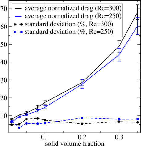
Figure 3: Normalized drag values for $Re_{p}=250,\,300$. Each data point corresponds to the mean value of $5$ runs. The standard deviation is shown as error bars and separately in percent. The percent values are strictly below $10\%$ and not correlated with the solid volume fraction.

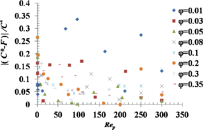
Figure 4: Pointwise relative deviation of the computed values $C^{*}$ from the fit correlation $F$ given by Eq. (15).

For the present study of the drag force within mono-disperse fixed assemblies of spheres, the solid volume fraction takes the values $\varphi\in$ $\{0.01,$ $0.03,$ $0.05,$ $0.08,$ $0.1,$ $0.2,$ $0.3,$ $0.35\}$, while the particle Reynolds number $Re_{p}$ is varied from $0.05$ to $300$. A series of simulations was carried out, repeating each pair $(\varphi,Re_{p})$ at least five times. In our approach, the average flow velocity in the domain may vary depending on the randomly generated bed. Hence, the resulting Reynolds numbers has also been averaged for each series. For higher target Reynolds numbers ($Re_{p}\geq 200$), however, the gravitation parameter $g$ was adjusted dynamically to fix the Reynolds number. The resolution in this study was varied between $d=17$ and $d=47$ lattice units per sphere diameter, and the number of spheres taken for each simulation was either $N=27$ or $N=54$. A cubic domain of length varying from 74 to 449 lattice units, depending on the desired volume fraction $\varphi$, was used with periodic boundary conditions for all the exterior boundaries. The domain length to particle diameter ratio varied between $3.43$ and $11.18$. For each run a randomized arrangement of spheres is generated, and the resulting dimensionless drag values are averaged over the whole series to obtain the approximated bed-independent dimensionless drag force. The number of 5 runs was found to be sufficient to even out artifacts from the random bed generation, in consistency with the reports by Hill et al. (2001a) and Tenneti et al. (2011). We did not apply any “check-reject-repeat” – strategy to eliminate any spikes in our data. The variation of the resulting absolute values is largest for higher $Re_{p}$. Fig. 3 shows the data for the two highest Reynolds numbers included in this study, and the standard deviation for each data point. The situation is similar for the lower Reynolds number, however with smaller absolute values.

A dimensionless drag correlation $F$ is obtained using the conjugate gradient method to minimize the objective function

$$E=\sum_{(\varphi,Re_{p})}\frac{|F-C^{*}|}{F},$$

between the correlation and the LBM simulated values $C^{*}$ (averaged over $5$ random beds) with an average absolute percentage error of $9.69\%$ compared with the simulated data and with a coefficient of determination $R^{2}=0.995$. Using the model function $F(\varphi,Re_{p})=(1-\varphi)^{a}[b+c{Re_{p}}^{d}+e(1+Re_{p})^{-f\varphi}+g(1+Re_{p})^{-h\varphi}]$, with parameters $a,b,..,h$, one obtains the correlation $C=F(\varphi,Re_{p})$, with

$$\begin{split}F=&(1-\varphi)^{-5.726}\big{[}1.751+0.151\,{Re_{p}}^{0.684}\\ &-0.445\,(1+Re_{p})^{1.04\varphi}-0.16\,(1+Re_{p})^{0.0003\varphi}\big{]}.\end{split}$$ (15)

Fig. 4 shows the pointwise deviation $|F-C^{*}|/C^{*}$ between Eq. (15) and the simulated values. One observes the largest deviations for small volume fractions. The average absolute percentage error with respect to $C^{*}$ is $9.3\%$. Unlike the correlations reported by other authors (for instance Beetstra et al., 2007; Benyahia et al., 2006), which consist of two parts; the first part for the Stokes region, i.e., $Re_{p}\ll 1$, and a function of volume fraction only; the second part a function of solid volume fraction and $Re_{p}$, we chose a unified expression.

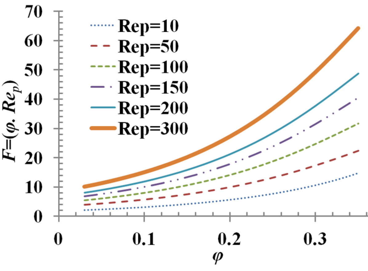
(a) Normalized drag force based on total hydrodynamic force as a function of solid volume fraction for different particle Reynolds number.

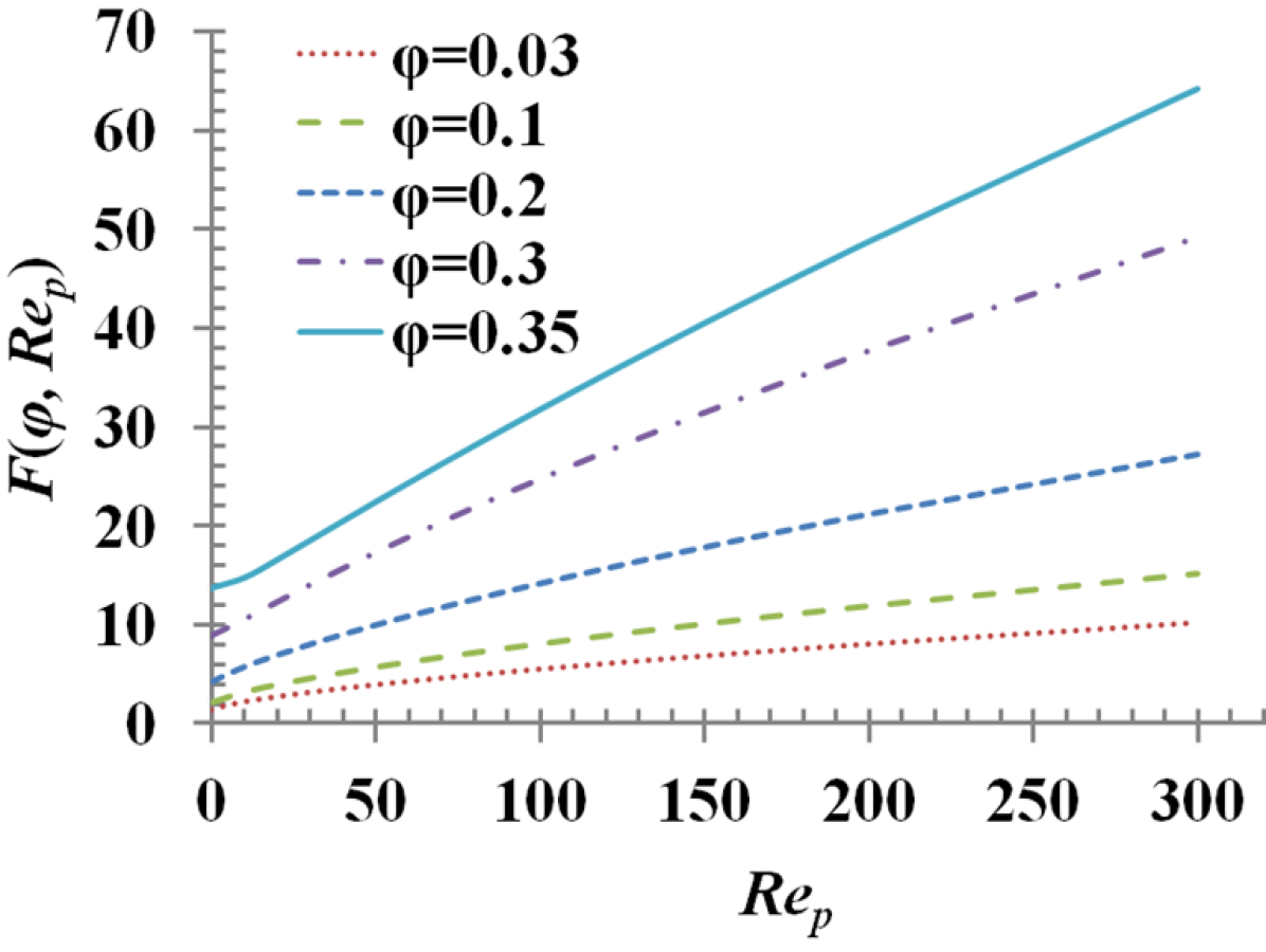
(b) The normalized drag force as a function of the Reynolds number $Re_{p}$ for various solid volume fractions.

Figure 5: Drag correlation derived from present study.

Fig. 5(a) shows the effect of $\varphi$ on the normalized drag force at constant Reynolds number. It can be seen that the increase in drag force with increase in $\varphi$ is more significant at high Reynolds number. Similarly, it can be seen from Fig. 5(b) that at a constant $\varphi$ the normalized drag force increases with the Reynolds number. The slope becomes steeper with increasing concentration $\varphi$. At low concentrations and Reynolds number beyond $Re_{p}>200$, the increase of drag with $Re_{p}$ is least significant.

3.5 Comparison with previous studies

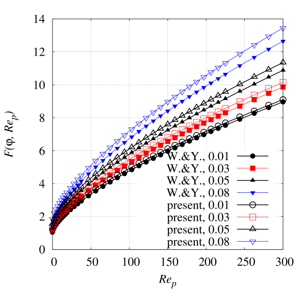
Figure 6: Wen & Yu - correlation for low solid volume fractions $\varphi=0.01\,..\,0.08$ (filled symbols) in comparison to the present study (hollow symbols).

At low solid volume fractions $\varphi\lesssim 0.2$, there is the well-established correlation by Wen and Yu (1966), compiled from experimental data. Because of the emphasis on the dilute case in our study, we compare to this relation first. Fig. 6 shows that the newly presented correlation is close to the Wen & Yu - relation for the most dilute cases included in this study. The smallest average deviation is $+4.3\%$ for $\varphi=0.01$, and increases with $\varphi$. The average deviation for $\varphi=0.2$ is $+10.8\%$ as shown in Fig. 7. Note, that the correlation given by Wen and Yu is applicable only for $\varphi\lesssim 0.2$, whereas the proposed correlation can be used up to $\varphi\approx 0.35$.

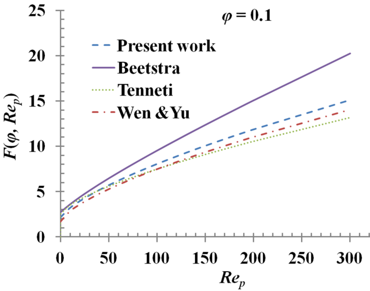
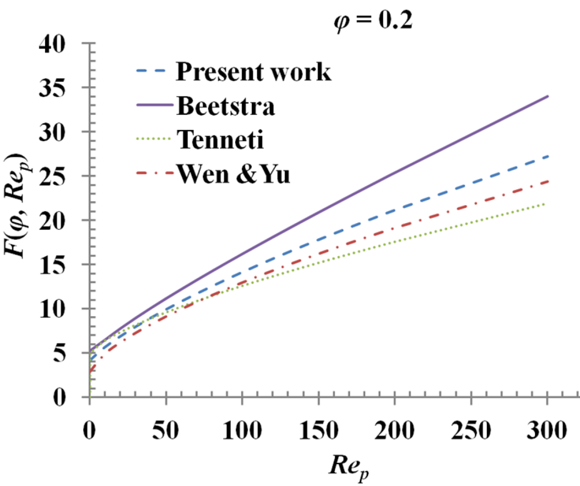
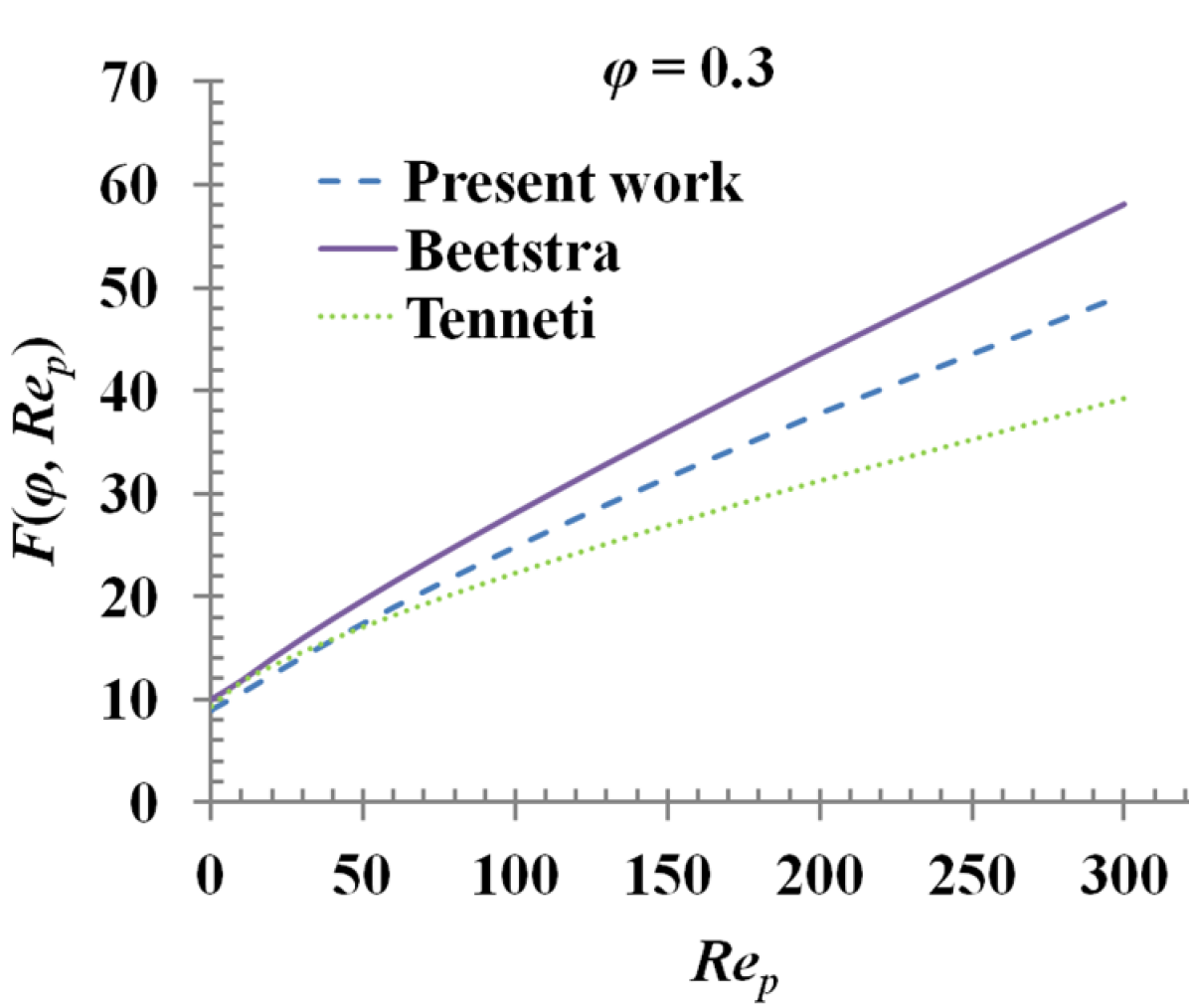
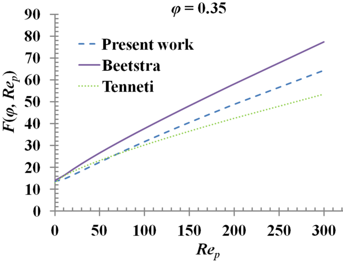
Figure 7: Normalized drag force predicted by our correlation compared to that reported by other authors.

Fig. 7 shows the drag law predicted by Eq. (15) in comparison to the correlations obtained in the numerical studies by Beetstra et al. (2007) and Tenneti et al. (2011). In these references, both the simulated hydrodynamic force and average flow rate is averaged over all runs of each $(\varphi,Re_{p})$ – pair, to therefrom obtain the unknown dimensionless drag. The maximum and minimum average deviation when compared with the drag law reported by Tenneti et al. (2011) is approximately $+12\%$ for $\varphi=0.2$, and $+7\%$ for $\varphi=0.35$, respectively. The deviation increases with the Reynolds number. When compared with the results reported by Beetstra et al. (2007), the maximum and minimum average deviation is approximately $-20\%$ for $\varphi=0.1$ and $-14\%$ for $\varphi=0.3$, respectively. Tenneti et al. (2011) comment that the deviation of more than $30\%$ between the values reported by Beetstra et al. (2007) and their own is due to the poor lattice resolutions applied in the latter work. Hence, of the two references, the study of Tenneti et al. (2011) should be regarded more accurate. The lattice resolutions for the present study are comparable those applied by Tenneti, and have been chosen based on the considerations of Sec. 3.2. The present LBM-scheme does not suffer from a viscosity dependent error at the solid boundaries. As we have also demonstrated numerically (cf. Tab. 3) for $Re=300$, where the deviation from the other studies was most significant, this deviation is independent from the parameterization according to Eq. (9). The sensitivity study of Sec. 3.2 indicates that errors due to unresolved flow phenomena do not affect the present study significantly. However, a small error stemming from the first-order staircase approximation of the sphere boundaries is present and can roughly be estimated to yield an overshoot of a few percent. We believe that the deviations between the present study and that of Tenneti et al. (2011) is partially due to that reason.

4 Conclusion

Fluid flow through random static assemblies of spheres has been studied by means of the lattice Boltzmann method. Compared with previous studies, our approach does not suffer from viscosity dependent boundary conditions. As a result, a wide range of Reynolds numbers can be studied by simple adjustment of the lattice viscosity - provided that a sufficient grid resolution is chosen. A convergence study demonstrates that the results are effectively independent of the lattice resolution. From systematic numerical studies of flow through random arrays at varying solid volume fraction ($0.01\leq\varphi\leq 0.35$), a new correlation for the average normalized drag force for particle Reynolds numbers up to $300$ is obtained.

Despite a certain expected error from the first order boundary conditions (“bounce back-rule”), we successfully showed the reliability of the present approach for the given range of moderate Reynolds numbers. The comparison with Wen and Yu (1966) shows that the correlation predicts well at very low concentrations ($\varphi<0.1$) and at the same time can be used up to a solid volume fraction of $0.35$. The deviations of the results obtained with our lattice Boltzmann scheme to the simulations of Tenneti et al. (2011) are not as dramatic as reported in the same reference in comparison to previous lattice Boltzmann studies. This confirms the reliability of the LBM. On the other hand, the existing deviations between different numerical approaches also indicate a need for further studies conducted with more accurate numerical schemes in the future, as it is presently unclear which results are the more reliable. This could be achieved by using a lattice Boltzmann method equipped with a higher order boundary scheme (Bouzidi et al., 2001; Ginzburg and d’Humieres, 2003; Mei et al., 2002), for instance.

The normalized drag correlation proposed in the present study will be useful in predicting the flow behavior of particles in fluid-particulate systems, where the solid volume fractions range from very low to moderate values. Usually, more than one correlations are used when the range of solid volume fraction and Reynolds number is large. The correlation proposed by us has a simpler expression compared to those proposed by, e.g., Beetstra et al. (2007) or Benyahia et al. (2006), and is purely based on LBM simulated data. Future work will aim at obtaining a correlation that can be used for higher solid volume fractions and higher Reynolds numbers.

References

- Aidun and Clausen (2010) C. K. Aidun and J. R. Clausen. Lattice-Boltzmann method for complex flows. Annu. Rev. Fluid Mech., 42:439–472, 2010.
- Beetstra et al. (2007) R. Beetstra, M. A. van der Hoef, and J. A. M. Kuipers. Drag force of intermediate Reynolds number flow past mono- and bidisperse arrays of spheres. Fluid Mechanics and Transport Phenomena, 53(2):489–501, 2007. doi: 10.1002/aic.11065.
- Benyahia et al. (2006) S. Benyahia, M. Syamlal, and T. J. O’Brien. Extension of Hill-Koch-Ladd - drag correlation over all ranges of Reynolds number and solids volume fraction. Powder Technology, 162:166–174, 2006.
- Benzi et al. (1992) R. Benzi, S. Succi, and M. Vergassola. The lattice Boltzmann equation: theory and applications. Physics Reports, 222(3):145–197, 1992.
- Bogner and Rüde (2013) S. Bogner and U. Rüde. Simulation of floating bodies with the lattice Boltzmann method. Computers and Mathematics with Applications, 65:901–913, 2013.
- Bouzidi et al. (2001) M. Bouzidi, M. Firdaouss, and P. Lallemand. Momentum transfer of a Boltzmann-lattice fluid with boundaries. Physics of Fluids, 13(11):3452, 2001.
- Buick and Greated (2000) J.M. Buick and C.A. Greated. Gravity in a lattice Boltzmann model. Phys. Rev. E, 61(5):5307, 2000.
- Chen and Doolen (1998) S. Chen and G. D. Doolen. Lattice Boltzmann method for fluid flows. Annu. Rev. Fluid Mech., 30:329–364, 1998.
- Chu et al. (2009) K. W. Chu, B. Wang, A. B. Yu, A. Vince, G. D. Barnett, and P. J. Barnett. CFD–DEM study of the effect of particle density distribution on the multiphase flow and performance of dense medium cyclone. Minerals Engineering, 22:893–909, 2009.
- d’Humieres and Ginzburg (2009) D. d’Humieres and I. Ginzburg. Viscosity independent numerical errors for lattice Boltzmann models: From recurrence equations to ”magic” collision numbers. Computers and Mathematics with Applications, 58:823–840, 2009.
- Ergun (1952) S. Ergun. Fluid flow through packed columns. Chemical Engineering Progress, 48:89–94, 1952.
- Feichtinger et al. (2011) C. Feichtinger, S. Donath, H. Köstler, J. Götz, and U. Rüde. WaLBerla: HPC software design for computational engineering simulations. Journal of Computational Science, 2(2):105–112, 2011. doi: 10.1016/j.jocs.2011.01.004.
- Gidaspow (1986) D. Gidaspow. Hydrodynamics of fluidization and heat transfer: supercomputer modeling. Applied Mechanics Review, 39:1–23, 1986.
- Ginzbourg and Adler (1994) I. Ginzbourg and P.M. Adler. Boundary flow condition analysis for three-dimensional lattice Boltzmann model. Journal of Physics II France, 4:191–214, 1994.
- Ginzburg (2005) I. Ginzburg. Equilibrium-type and link-type lattice Boltzmann models for generic advection and anisotropic-dispersion equation. Advances in Water Resources, 28:1171–1195, 2005.
- Ginzburg and d’Humieres (2003) I. Ginzburg and D. d’Humieres. Multireflection boundary conditions for lattice Boltzmann models. Physical Review E, 68:066614–1 – 066614–29, 2003.
- Ginzburg et al. (2008) I. Ginzburg, F. Verhaeghe, and D. d’Humieres. Two-relaxation-time lattice Boltzmann scheme: About parametrization, velocity, pressure and mixed boundary conditions. Communications in Computational Physics, 3(2):427–478, 2008.
- Götz et al. (2010) J. Götz, K. Iglberger, M. Stürmer, and U. Rüde. Direct numerical simulation of particulate flows on 294912 processor cores. In Proceedings of the 2010 ACM/IEEE International Conference for High Performance Computing, Networking, Storage and Analysis, pages 1–11. IEEE Computer Society, 2010.
- Guo et al. (2002) Z. Guo, Chuguang Zheng, and Baochang Shi. Discrete lattice effects on the forcing term in the lattice Boltzmann method. PHYSICAL REVIEW E, 65:046308–1 – 046308–6, 2002.
- Hasimoto (1959) H. Hasimoto. On the periodic fundamental solutions of the Stokes equations and their application to viscous flow past a cubic array of spheres. Journal of Fluid Mechanics, 5:317–328, 1959.
- Hill et al. (2001a) R. J. Hill, D. L. Koch, and A. J. C. Ladd. The first effects of fluid inertia on flows in ordered and random arrays of spheres. Journal of Fluid Mechanics, 448:213–241, 2001a. doi: 10.1017/S0022112001005948.
- Hill et al. (2001b) R. J. Hill, D. L. Koch, and A. J. C. Ladd. Moderate-Reynolds-number flows in ordered and random arrays of spheres. Journal of Fluid Mechanics, 448:243–278, 2001b. doi: 10.1017/S0022112001005936.
- Holloway et al. (2010) W. Holloway, X. Yin, and S. Sundaresan. Fluid-particle drag in inertial polydisperse gas-solid suspensions. American Institute of Chemical Engineers Journal, 56(8):1995–2004, 2010.
- Junk and Yang (2005) M. Junk and Z. Yang. Asymptotic analysis of lattice boltzmann boundary conditions. Journal of Statistical Physics, 121 (1/2):3–35, 2005.
- Ladd (1994a) A.-J.-C. Ladd. Numerical simulations of particulate suspensions via a discretized Boltzmann equation. Part 1. Theoretical foundation. Journal of Fluid Mechanics, 271:285–309, July 1994a.
- Ladd (1994b) A.-J.-C. Ladd. Numerical simulations of particulate suspensions via a discretized Boltzmann equation. Part 2. Numerical results. Journal of Fluid Mechanics, 271:311–339, July 1994b.
- Ladd and Verberg (2001) A. J. C. Ladd and R. Verberg. Lattice-Boltzmann simulations of particle-fluid suspensions. Journal of Statistical Physics, 104:1191–1251, 2001.
- Luo (1998) L.-S. Luo. Unified theory of lattice Boltzmann models for nonideal gases. Phys. Rev. Lett., 81(8):1618, 1998.
- Mei et al. (2002) R. Mei, D. Yu, W. Shyy, and L.-S. Luo. Force evaluation in the lattice Boltzmann method involving curved geometry. Phys. Rev. E, 65:041203, Apr 2002.
- Mishra and Tripathy (2010) B. K. Mishra and A. Tripathy. Preliminary study of particle separation in spiral concentrators using dem. International Journal of Mineral Processing, 94:192–195, 2010.
- Mohanty et al. (2011) S. Mohanty, B. Das, and B.K. Mishra. A preliminary investigation into magnetic separation process using cfd. Minerals Engineering, 24:1651–1657, 2011.
- Pan et al. (2006) C. Pan, L.-S. Luo, and C. T. Miller. An evaluation of lattice Boltzmann schemes for porous medium flow simulation. Computers & Fluids, 25:898–909, 2006.
- Qian et al. (1992) Y. H. Qian, D. d’Humieres, and P. Lallemand. Lattice BGK models for Navier-Stokes equations. Europhysical Letters, 17(6):479–484, 1992.
- Richardson and Zaki (1954) J. F. Richardson and W. N. Zaki. Sedimentation and fluidisation. part i. Transactions of the Institution of Chemical Engineers, 32:35–53, 1954.
- Sangani and Acrivos (1982) A. S. Sangani and A. Acrivos. Slow flow through a periodic array of spheres. International Journal of Multiphase Flow, 8(4):343–360, 1982.
- Shyamlal and O’Brien (1987) M. Shyamlal and T. J. O’Brien. A generalized drag correlation for multiparticle systems. Morgantown Energy Technology Center DOE Report, 1987.
- Succi (2001) S. Succi. The Lattice Boltzmann Equation for Fluid Dynamics and Beyond. Oxford Science Publications, 2001.
- Swain and Mohanty (2013) S. Swain and S. Mohanty. A 3-dimensional Eulerian-Eulerian CFD simulation of a hydrocyclone. Applied Mathematical Modelling, 37:2921–2932, 2013.
- Tenneti et al. (2011) S. Tenneti, R. Garg, and S. Subramaniam. Drag law for monodisperse gas-solid systems using particle-resolved direct numerical simulation of flow past fixed assemblies of spheres. International Journal of Multiphase Flow, 37:1072–1092, 2011.
- van der Hoef et al. (2005) M. A. van der Hoef, R. Beetstra, and J. A. M. Kuipers. Lattice-Boltzmann simulations of low-Reynolds-number flow past mono- and bidisperse arrays of spheres: results for the permeability and drag force. Journal of Fluid Mechanics, 528:233–254, 2005. doi: 10.1017/S0022112004003295.
- van der Hoef et al. (2006) M. A. van der Hoef, M. Ye, M. van Sint Annaland, A. T. Andrews, S. Sundaresan, and J. A. M. Kuipers. Multiscale modeling of gas-fluidized beds. Advances in Chemical Engineering, 31:64–149, 2006.
- Wen and Yu (1966) C. Y. Wen and Y. H. Yu. Mechanics of fluidization. Chem Eng Prog Symp Ser., 62:100–111, 1966.
- Yin and Sundaresan (2009a) X. Yin and S. Sundaresan. Drag law for bidisperse gas-solid suspensions containing equally sized spheres. Industrial and Engineering Chemistry Research, 48:227–241, 2009a.
- Yin and Sundaresan (2009b) X. Yin and S. Sundaresan. Fluid-particle drag in low-Reynolds-number polydisperse gas-solid suspensions. American Institute of Chemical Engineers Journal, 55:1352–1368, 2009b.
- Yu et al. (2003) D. Yu, R. Mei, L.-S. Luo, and W. Shyy. Viscous flow computations with the method of lattice Boltzmann equation. Progress in Aerospace Sciences, 39:329–367, 2003.