Analysis and simulations
of multifrequency induction hardening

Abstract

We study a model for induction hardening of steel. The related differential system consists of a time domain vector potential formulation of the Maxwell’s equations coupled with an internal energy balance and an ODE for the volume fraction of austenite, the high temperature phase in steel. We first solve the initial boundary value problem associated by means of a Schauder fixed point argument coupled with suitable a-priori estimates and regularity results. Moreover, we prove a stability estimate entailing, in particular, uniqueness of solutions for our Cauchy problem. We conclude with some finite element simulations for the coupled system.

1 Introduction

In induction hardening a coil that is connected to an alternating current source generates a periodically changing electro-magnetic field. The temporal changing magnetic flux induces a current in the workpiece that is enclosed by the induction coil. Due to the resistance of the workpiece, some part of the power is transformed into eddy current losses that result in Joule heating. The latter leads to a change of microstructure to the high temperature phase in steel called austenite. After switching off the current and possibly a short holding time the workpiece is cooled rapidly and the austenite layer produced upon heating is transformed to another phase called martensite, responsible for the desired hardening effect.

Induction heat treatments can easily be integrated into a process chain. Moreover, they are energy efficient since the heat is generated directly in the workpiece. That is why induction hardening is still the most important surface treatment technology.

Due to the skin effect, the eddy currents tend to distribute in a small surface layer. The penetration depth of these eddy currents depends on the material and essentially on the frequency. Therefore, it is difficult to obtain a uniform contour hardened zone for complex workpiece geometries such as gears using a current with only one frequency. If for example, a high frequency (HF) is applied, then the penetration depth is small and it is possible to harden only the tip of the gear. With a medium frequency (MF) it is possible to heat the root of the gear, but not the tip. With a single frequency, a hardening of the complete tooth can only be achieved by increasing the heating time. But then, the complete tooth is heated beyond the austenitization temperature, which results in a complete martensitic structure of the tooth after quenching, which is not desirable, since this will foster fatigue effects.

Recently, a new approach has been developed which amounts to supplying medium and high frequency powers simultaneously on the induction coil. This concept is called multifrequency induction hardening, see also Figure 1.

Figure 1: The effect of medium-, high- and multifrequency induction heating. MF (left): only the root of the gear is heated, HF (middle): only the tip of the gear is heated, MF+HF (right): tip and root of the gear are heated.

The inductor current consists of a medium frequency fundamental oscillation superimposed by a high frequency oscillation. The amplitudes of both frequencies are independently controllable, which allows separate regulation of the respective shares of the output power of both frequencies according to the requirements of the workpiece. This provides the ability to control the depth of hardening at the root and the tip of the tooth individually [19].

The main building blocks for a mathematical model of multifrequency hardening are an eddy current formulation of the Maxwell equations in the time domain, coupled to the balance of internal energy to describe the temperature evolution, and a model for the evolution of the high temperature phase austenite. Since the electric conductivity and the magnetic permeability may depend on temperature and/or the phase fractions and the Joule effect in the time domain is modelled by the square of the time derivative of the magnetic vector potential we are faced with a strongly coupled nonlinear system of evolution equations.

In two recent papers the simpler frequency domain situation of Joule heating has been studied. In [8] the Boccardo-Galluet approach has been used to prove existence of a weak solution, while in [4] new regularity results established in [3] have been used to prove existence and stability in the frequency domain setting. In [11, 12] the eddy current model has been considered in the time domain. In the former the existence of a weak solution to the fully coupled model has been proven, in the latter also stability results are established, but only for a model with one-sided coupling in which the electric conductivity and permeability are assumed to be constant.

The main novelty of the present paper is an existence and stability result for the strongly coupled time domain eddy current and Joule heating system. The paper is organised as follows. In the next section we derive the model equations and show that it complies with the second law of thermodynamics in form of the Clausius-Duhem inequality. In Section 3 we formulate the main mathematical results, the proofs of which are given in Section 4. The last section is devoted to presenting some results of numerical simulations for the coupled system based on a two time step approach with sequential decoupling of the evolution equations.

2 The model

We restrict to the following idealized geometric setting (cf. the following Figure 2). Let $D\in\mathbb{R}^{3}$ be a domain containing the inductor coil $\Omega$ and the workpiece $\Sigma$. Assume that $\overline{\Omega}\subset D$, $\overline{\Sigma}\subset D$, $\overline{\Omega}\cap\overline{\Sigma}=\emptyset$ and $\partial\Omega$, $\partial\Sigma$, $\partial D$ are of class $C^{1,1}$. Call $G=\Omega\cup\Sigma$ the set of conductors and define the space-time domain as $Q=\Sigma\times(0,T)$.

\begin{overpic}[width=142.26378pt]{gebiet2.png} \put(50.0,50.0){$\Sigma$} \put(30.0,30.0){$D$} \put(70.0,40.0){$\Omega$} \end{overpic}

Figure 2: Domain $D$ consisting of the inductor $\Omega$, the workpiece $\Sigma$ and the surrounding air.

Following the model derivation of [11], in the eddy current problems we neglect displacement currents and so we get the following Maxwell’s equations (cf. [2]) in $D\times(0,T)$:

(2.1) $$\operatorname{curl}H=J,$$

(2.2) $$\operatorname{curl}E=-B_{t},$$

(2.3) $$\operatorname{div}B=0\,,$$

where $E$ is the electric field, $B$ the magnetic induction, $H$ the magnetic field, $J$ the spatial current density.

We include phase transitions by describing the evolution of the volume fraction of austenite $z$ with the following problem derived in [15] and [6]:

(2.4) $$z_{t}(t)=\frac{\left(z_{eq}(\vartheta)-z\right)^{+}}{\tau(\vartheta)}\quad\hbox{in }Q\,,$$

$$z(0)=0\quad\hbox{in }\Sigma\,.$$

We will make precise the assumption on $\tau$ and $z_{eq}$ in the following section, however note that $z_{eq}\in[0,1]$ is an equilibrium fraction of austenite, $\tau(\vartheta)$ a time constant, and by $(\cdot)^{+}$ we denote the positive part function.

Then, we assume the Ohm’s law and a linear relation between the magnetic induction and the magnetic field in $D\times(0,T)$:

(2.5) $$J=\sigma E\,,$$

$$B=\mu H\,,$$

where the electrical conductivity $\sigma$ and the magnetic permeability $\mu$ (sufficiently regular and bounded from below and above) may depend both on the spatial variables and also on the phase parameter $z$ and on the absolute temperature $\vartheta$:

(2.6) $$\sigma(x,z,\vartheta)=\begin{cases}0,\quad&x\in D\setminus G\,,\\ \sigma_{w}(z,\vartheta),\quad&x\in\Sigma\,,\\ \sigma_{i},\quad&x\in\Omega\,,\end{cases}$$

with its derivative with respect to the $z$-variable

(2.7) $$\sigma_{z}(x,z,\vartheta)=\begin{cases}0,\quad&x\in D\setminus\Sigma\,,\\ \sigma_{w}^{\prime}(z,\vartheta),\quad&x\in\Sigma\,,\end{cases}$$

and

(2.8) $$\mu(x,z,\vartheta)=\begin{cases}\mu_{0},\quad&x\in D\setminus G\,,\\ \mu_{w}(z,\vartheta),\quad&x\in\Sigma\,,\\ \mu_{i},\quad&x\in\Omega\,,\end{cases}$$

with

(2.9) $$\mu_{z}(x,z,\vartheta)=\begin{cases}0,\quad&x\in D\setminus\Sigma\,,\\ \mu_{w}^{\prime}(z,\vartheta),\quad&x\in\Sigma\,.\end{cases}$$

In view of (2.3), we introduce the magnetic vector potential $A$ such that

(2.10) $$B=\operatorname{curl}A\quad\hbox{in }D$$

and, since $A$ is not uniquely defined, we impose the Coulomb gauge

$$\operatorname{div}A=0\quad\hbox{in }D\,.$$

Using (2.2) and (2.10), we define the scalar potential $\phi$ by

(2.11) $$E+A_{t}=-\nabla\phi\quad\hbox{in }D\times(0,T)\,.$$

Using (2.5), we then obtain the following form for the total current density

(2.12) $$J=-\sigma A_{t}-\sigma\nabla\phi\quad\hbox{in }D\times(0,T)\,,$$

which, together with (2.10) and (2.1), gives

(2.13) $$\sigma A_{t}+\operatorname{curl}\left(\frac{1}{\mu}\operatorname{curl}A\right)=J_{source}\quad\hbox{in }D\times(0,T)\,,$$

where, for a given coil geometry (here a torus with rectangular cross-section), the source current density

(2.14) $$J_{source}=-\sigma\nabla\phi$$

can be precomputed analytically and it can be used as control for optimization, i.e., it can be taken of the form $J_{source}=u(t)J_{0}$, where $J_{0}$ is the spatial current density prescribed in the induction coil $\Omega$

(2.15) $$J_{0}(x)=\begin{cases}J_{i}(x),\quad&x\in\Omega\\ 0,\quad&x\in D\setminus\Omega\,,\end{cases}$$

and $u=u(t)$ denotes a time-dependent control on $[0,T]$. Assuming to have as constant density $\rho=1$ (for simplicity), the internal energy balance in $Q$ results as

(2.16) $$e_{t}+\operatorname{div}q=JE=\sigma|A_{t}+\nabla\phi|^{2}=\sigma|A_{t}|^{2}\,,$$

where $e$ denotes the internal energy of the system and $q$ the heat flux, which, accordingly to the standard Fourier law is assumed as follows

(2.17) $$q=-\kappa(\vartheta)\nabla\vartheta,\quad\kappa>0\,.$$

In case $\kappa(\vartheta)=\kappa>0$ constant, we get the standard Fourier law. From the Helmholtz relation $e=\psi+\vartheta s$, where $\psi=\psi(\vartheta,z)$ denotes the free energy of the system, (2.16) and (2.17), we have that the Clausius-Duhem inequality

(2.18) $$\vartheta\left(s_{t}+\operatorname{div}\left(\frac{q}{\vartheta}\right)\right) =e_{t}-\psi_{\vartheta}\vartheta_{t}-\psi_{z}z_{t}-\vartheta_{t}s-\frac{q}{\vartheta}\nabla\vartheta+\operatorname{div}q$$

$$=e_{t}+\operatorname{div}q-(\psi_{\vartheta}+s)\vartheta_{t}-\psi_{z}z_{t}+\frac{\kappa|\nabla\vartheta|^{2}}{\vartheta}$$

$$=\sigma|A_{t}|^{2}-(\psi_{\vartheta}+s)\vartheta_{t}-\psi_{z}z_{t}+\frac{\kappa|\nabla\vartheta|^{2}}{\vartheta}$$

$$\geq 0$$

is satisfied e.g. if we assume the standard relations $\psi_{\vartheta}+s=0$ and $L\tau(\vartheta)z_{t}=-\psi_{z}$, and hence (cf.(2.4)) $\psi_{z}=-L(z_{eq}(\vartheta)-z)^{+}$, for some positive constant $L>0$. Then, using the definition of the specific heat $c_{v}=\vartheta s_{\vartheta}$ (cf., e.g., [16]), we get

$$e_{t}=c_{v}\vartheta_{t}+(\psi_{z}+\vartheta s_{z})z_{t}=c_{v}\vartheta_{t}+\mathcal{F}(\vartheta,z)z_{t}\,,$$

where we have denoted for simplicity by

(2.19) $$\mathcal{F}(\vartheta,z)=\psi_{z}-\vartheta(\psi_{z})_{\vartheta}=-L(z_{eq}(\vartheta)-z)^{+}+L\vartheta z_{eq}^{\prime}(\vartheta)\mathcal{H}(z_{eq}(\vartheta)-z)\,.$$

Here $\mathcal{H}$ represents the Heaviside function. Hence, the internal energy balance (2.16) can be rewritten as

(2.20) $$c_{v}\vartheta_{t}+\operatorname{div}q=\sigma|A_{t}|^{2}-\mathcal{F}(\vartheta,z)z_{t}\quad\hbox{in }Q.$$

Finally, we couple the system (2.4), (2.13), (2.14), (2.17), (2.19–2.20) with suitable boundary conditions. We assume that the tangential component of $A$ vanishes on $\partial D$, i.e.

(2.21) $$n\times A=0\quad\hbox{on }\partial D\times(0,T)\,,$$

where $n$ denotes the outward unit normal vector to $\partial D$; for the absolute temperature we neglect the possible radiative heat transfer between the inductor and the workpiece assuming

(2.22) $$\kappa\frac{\partial\vartheta}{\partial\nu}+\eta\vartheta=g\quad\hbox{on }\partial\Sigma\times(0,T)\,,$$

where $\nu$ denotes the outward unit normal vector to $\partial\Sigma$, $\eta$ stands for an heat transfer coefficient and $g$ is a given boundary source.

In the following sections we will study the well-posedness for the Cauchy system associated to a suitable variational formulation of (2.4), (2.13), (2.14), (2.17), (2.19–2.22).

3 Well-posedness results

In this section we introduce the functional framework, the main notation, and the assumptions on the data in order to deal with system (2.4), (2.13), (2.14), (2.17), (2.19–2.22). Moreover, we state here our main results concerning well-posedness and regularity for a suitable weak formulation of the corresponding Cauchy problem. The proofs of these results are given in Section 4. For analytical reasons our analysis is restricted to the case $\sigma=\sigma(x,z)$, $\mu=\mu(x,z)$ in (2.6) and (2.8), that is we drop the explicit temperature dependence. Since the phase fraction grows with growing temperature we still maintain the effect of temperature change on the parameter values. Moreover, we consider the standard Fourier law with $\kappa$ positive constant in (2.17).

3.1 Notation and preliminaries

We first recall the definitions of generalized $\operatorname{curl}$ and $\operatorname{div}$ operators as well as the related embedding results we need in the sequel. Referring to the Figure 2, let $D\subseteq\mathbb{R}^{3}$ be a bounded domain. Assume that $\overline{\Omega}\subset D$, $\overline{\Sigma}\subset D$, $\overline{\Omega}\cap\overline{\Sigma}=\emptyset$ and $\partial\Omega$, $\partial\Sigma$, $\partial D$ are of class $C^{1,1}$. Define $G=\Omega\cup\Sigma$ and the space-time domain $Q=\Sigma\times(0,T)$. Let us denote with the symbol $\mathbb{W}$ the vector-valued counterpart of the Banach space $W$. Let us use the symbol $\mathbb{L}^{q}(U\times(0,t))$ for the space $L^{q}(0,t;\mathbb{L}^{q}(U))$, for every $q\in[1,+\infty)$, $t\in(0,T]$, $U$ bounded and $C^{1,1}$ domain in $\mathbb{R}^{3}$. Let $p\in(1,+\infty)$ and $\psi\in\mathbb{L}^{p}(D)$, then, we write $\operatorname{curl}\psi\in\mathbb{L}^{p}(D)$ if there exists $\xi\in\mathbb{L}^{p}(D)$ such that

$$\int_{D}\psi\operatorname{curl}\phi\;\!\mathrm{d}x=\int_{D}\xi\phi\;\!\mathrm{d}x\,,$$

for all $\phi\in\mathbb{C}^{\infty}_{c}(D)$. We define $\operatorname{curl}\psi:=\xi$, as the uniquely determined vector $\xi$. Analogously, we write $\operatorname{div}\psi\in L^{p}(D)$ if there exists $\zeta\in L^{p}(D)$ such that

$$\int_{D}\psi\cdot\nabla\eta\;\!\mathrm{d}x=-\int_{D}\zeta\eta\;\!\mathrm{d}x\,,$$

for all $\eta\in C^{\infty}_{c}(D)$. We define $\operatorname{div}\psi:=\zeta$, as the uniquely determined vector $\zeta$. Then, we introduce the Banach spaces (with the graph norms) $\mathbb{L}^{p}_{curl}(D)=\{\psi\in\mathbb{L}^{p}(D)\,:\,\operatorname{curl}\psi\in\mathbb{L}^{p}(D)\}$ and $\mathbb{L}^{p}_{div}(D)=\{\psi\in\mathbb{L}^{p}(D)\,:\,\operatorname{div}\psi\in L^{p}(D)\}$. For $\psi\in L^{2}_{curl}(D)$ we define the the linear bounded trace operator $\gamma_{\tau}(\psi)$ using the well-known Green’s formula (cf., e.g. [5])

(3.1) $$\int_{D}\psi\operatorname{curl}\phi\;\!\mathrm{d}x-\int_{D}\operatorname{curl}\psi\cdot\phi\;\!\mathrm{d}x=-\int_{\partial D}(n\times\psi)\cdot\phi\;\!\mathrm{d}s=:\langle{\gamma_{\tau}(\psi),\phi}\rangle\,,$$

for all $\phi\in\mathbb{H}^{1}(D)$, where (with an abuse of notation) the integral over $\partial D$ has to be understood as the duality between $\mathbb{H}^{-1/2}(\partial D)$ and $\mathbb{H}^{1/2}(\partial D)$ and $n$ denotes the outward unit normal vector to $\partial D$. Similarly, for $\psi\in L^{2}_{div}(D)$ we introduce the linear bounded trace operator $\gamma_{n}(\psi)$ by the Green’s formula

(3.2) $$\int_{D}\psi\cdot\nabla\phi\;\!\mathrm{d}x+\int_{D}\operatorname{div}\psi\cdot\phi\;\!\mathrm{d}x=\int_{\partial D}(n\cdot\psi)\phi\;\!\mathrm{d}s=:\langle{\gamma_{n}(\psi),\phi}\rangle\,,$$

for all $\phi\in H^{1}(D)$, where (with an abuse of notation) the integral over $\partial D$ has to be understood as the duality between $H^{-1/2}(\partial D)$ and $H^{1/2}(\partial D)$. Finally, we introduce the Hilbert space

$$\mathbb{X}=\{v\in\mathbb{L}^{2}_{curl}(D)\,:\,\operatorname{div}v=0\quad\hbox{and }\gamma_{\tau}(v)=0\}\,.$$

Notice that, since $\partial D\in C^{1,1}$, then the space $\mathbb{X}$, equipped with the norm

$$\|v\|_{\mathbb{X}}=\|\operatorname{curl}v\|_{\mathbb{L}^{2}(D)}\,,$$

is a closed subspace of $\mathbb{H}^{1}(D)$. Moreover, let us notice that, from the Green’s formula it follows that: if $A\in\mathbb{X}$, then $\gamma_{n}(A)=0$. Indeed, if we denote by $w=\operatorname{curl}A\in\mathbb{L}^{2}(D)$, then $\operatorname{div}w=0$ and $\gamma_{n}(w)\in H^{-1/2}(\partial D)$. Moreover the following Green’s formulas hold true for every test function $\phi\in H^{1}(D)$:

(3.3) $$\langle{\gamma_{n}(w),\phi}\rangle= \int_{D}\left(\operatorname{div}w\phi+w\cdot\nabla\phi\right)\;\!\mathrm{d}x=\int_{D}\operatorname{curl}A\cdot\nabla\phi\;\!\mathrm{d}x$$

$$= \int_{D}\operatorname{curl}A\cdot\nabla\phi-\int_{D}A\cdot\operatorname{curl}\nabla\phi\;\!\mathrm{d}x$$

$$= \langle{\gamma_{\tau}(A),\nabla\phi}\rangle\,.$$

Hence, if $A\in\mathbb{X}$, then $\gamma_{n}(\operatorname{curl}A)=0$ (cf., e.g., [7, Chapter 2]).

We recall here some results which will be useful in the sequel of the paper. The first one is an embedding result which is a consequence of [9, Thm. 3.3]. The complete proof of a more general result can be found in [3, Prop. 2.2, p. 7].

Lemma 3.1.

Let $U\subset\mathbb{R}^{3}$ be a bounded $C^{1}$ domain, then the space

$$\mathcal{W}^{p,\alpha}(U)=\{u\in\mathbb{L}^{p}_{curl}(U)\cap\mathbb{L}^{p}_{div}(U)\,:\,\gamma_{n}(u)\in L^{\alpha}(\partial U)\}$$

continuously embeds in the space $\mathbb{L}^{\xi}(U)$ for $\xi:=\min\{\frac{3\alpha}{2},p^{*}\}$, where $p^{*}$ is the Sobolev embedding exponent

$$p^{*}:=\begin{cases}\frac{3p}{3-p}\quad&\hbox{if }1\leq p<3\,,\\ s\in[1,+\infty)\quad&\hbox{if }p=3\,,\\ +\infty\quad&\hbox{if }p>3\,.\end{cases}$$

Moreover, we recall the following interpolation inequality, holding true for $p,q,r\in[1,+\infty]$, with $p<r<q$, $1/r=\alpha/p+(1-\alpha)/q$, $\alpha\in(0,1)$, and $v\in\mathbb{L}^{q}(D)$:

(3.4) $$\|v\|_{\mathbb{L}^{r}(D)}\leq\|v\|_{\mathbb{L}^{p}(D)}^{\alpha}\|v\|_{\mathbb{L}^{q}(D)}^{1-\alpha}\,.$$

3.2 Hypotheses

We list here our basic assumptions on the functions $\sigma$, $\mu$, $J_{0}$, $u$, $\tau$, and $z_{eq}$ in (2.13), (2.4), and (2.20), where we take the constants $c_{v}$, $\kappa$, $\eta$, and $L$ equal to 1, for simplicity.

Hypothesis 3.2.

Assume that

• $\sigma(x,z)\,:\,\overline{D}\times[0,1]\to\mathbb{R}$ is a continuous and Lipschitz continuous (w.r.t. $z$ for almost all $x\in D$) function defined in (2.6) and (2.7), where $\sigma_{w}\in C^{1,1}([0,1])$, $\sigma_{i}>0$, constant. Assume moreover that there exists two constants $0<\underline{\sigma}\leq\overline{\sigma}$ such that

  $$\underline{\sigma}\leq\sigma(x,z)\leq\overline{\sigma}\quad\hbox{in }\overline{D}\times[0,1]\,;$$

• $\mu(x,z)\,:\,\overline{D}\times[0,1]\to\mathbb{R}$ is a continuous and Lipschitz continuous (w.r.t. $z$ for almost all $x\in D$) function defined in (2.8), (2.9), where $\mu_{w}\in C^{1,1}([0,1])$, $\mu_{i},\,\mu_{0}\in\mathbb{R}^{+}$. Assume moreover that there exists two constants $0<\underline{\mu}\leq\overline{\mu}$ such that

  $$\underline{\mu}\leq\mu(x,z)\leq\overline{\mu}\quad\hbox{in }\overline{D}\times[0,1]\,;$$

• $u\in H^{1}(0,T)$, $J_{0}\,:\,D\to\mathbb{R}^{3}$ is an $\mathbb{L}^{2}_{curl}(D)$-function defined in (2.15);

• $\tau,\,z_{eq}\in C^{2}(\mathbb{R})$ and there exists positive constants $0<\tau_{*}\leq\tau^{*}$ and $M>0$ such that

  $$\tau_{*}\leq\tau(\vartheta)\leq\tau^{*},\,0\leq z_{eq}(\vartheta)\leq 1\,\hbox{ for all }\vartheta\in\mathbb{R},\,\|\tau\|_{C^{2}(\mathbb{R})}\leq M,\,\|z_{eq}\|_{C^{2}(\mathbb{R})}\leq M\,,$$

  $$|-z_{eq}(\vartheta)+\vartheta z_{eq}^{\prime}(\vartheta)|\leq M\quad\hbox{for all }\vartheta\in\mathbb{R},\quad|\vartheta z_{eq}^{\prime\prime}(\vartheta)|\leq M\,;$$

• $g\in L^{\infty}(0,T;L^{\infty}(\partial\Sigma))$;

• $A_{0}\in\mathbb{X}\cap\mathbb{H}^{3}(D)$, $\vartheta_{0}\in W^{2,5/3}(\Sigma)$.

Remark 3.3.

We will use in the following weak formulation (3.10) of the internal energy balance (2.20) the notation $f(\vartheta,z)=-L(z_{eq}(\vartheta)-z-\vartheta z^{\prime}_{eq}(\vartheta))$. Indeed, using (2.4) we can rewrite $-\mathcal{F}(\vartheta,z)z_{t}=-f(\vartheta,z)z_{t}$ for $z\geq z_{eq}(\vartheta)$ and $-\mathcal{F}(\vartheta,z)z_{t}=0=-f(\vartheta,z)z_{t}$ for $z<z_{eq}(\vartheta)$. Notice moreover that Hyp. 3.2 (iv) implies that

(3.5) $$f\in C^{0,1}(\mathbb{R}\times[0,1]),\quad|f(\vartheta,z)|\leq C_{f}\quad\forall(\vartheta,z)\in\mathbb{R}\times[0,1]\,,$$

for some positive constant $C_{f}$ depending on $M$. Finally, let us observe that the assumption (3.5) are the only ones we need in order to get our next results, i.e., we do not need the explicit form (2.19) of $f$ which was assumed in the previous section in order to comply with Thermodynamics. However, other thermodynamically-compatible choices are possible.

3.3 Weak formulation and main theorem.

We are ready now to state the weak formulation of the Cauchy problem (2.4), (2.13), (2.14), (2.17), (2.19–2.22).

Problem 3.4.

Find a triple $(A,\vartheta,z)$ with the regularity properties

(3.6) $$A\in H^{2}(0,T;\mathbb{L}^{2}(D))\cap W^{1,\infty}(0,T;\mathbb{X}),\quad\operatorname{curl}A\in L^{\infty}(0,T;\mathbb{L}^{6}(D))\,,$$

(3.7) $$\vartheta\in W^{1,5/3}(0,T;L^{5/3}(\Sigma))\cap L^{5/3}(0,T;W^{2,5/3}(\Sigma))\cap L^{2}(0,T;H^{1}(\Sigma))\cap L^{\infty}(Q)\,,$$

(3.8) $$z\in W^{1,\infty}(0,T;W^{1,^{\infty}}(\Sigma)),\quad 0\leq z<1\hbox{ a.e. in }Q\,,$$

solving the following system

(3.9) $$\int_{G}\sigma(x,z)A_{t}\cdot v\;\!\mathrm{d}x+\int_{D}\frac{1}{\mu(x,z)}\operatorname{curl}A\cdot\operatorname{curl}v\;\!\mathrm{d}x=\int_{\Omega}J_{0}(x)u(t)\cdot v\;\!\mathrm{d}x$$

$$\qquad\qquad\qquad\qquad\hbox{ for all }v\in\mathbb{X},\hbox{ a.e. in }(0,T)\,,$$

(3.10) $$\vartheta_{t}-\Delta\vartheta=-f(\vartheta,z)z_{t}+\sigma(x,z)|A_{t}|^{2}\quad\hbox{a.e. in }Q\,,$$

(3.11) $$z_{t}=\frac{1}{\tau(\vartheta)}\left(z_{eq}(\vartheta)-z\right)^{+}\quad\hbox{a.e. in }Q\,,$$

(3.12) $$\frac{\partial\vartheta}{\partial\nu}+\vartheta=g\quad\hbox{a.e. on }\partial\Sigma\times(0,T)\,,$$

(3.13) $$A(0)=A_{0},\quad\hbox{a.e. in }D,\quad\vartheta(0)=\vartheta_{0},\quad z(0)=0\quad\hbox{a.e. in }\Sigma\,.$$

and satisfying the following estimate

(3.14) $$\|A\|_{H^{2}(0,T;\mathbb{L}^{2}(D))\cap W^{1,\infty}(0,T;\mathbb{X})}+\|\operatorname{curl}A\|_{L^{\infty}(0,T;\mathbb{L}^{6}(D))}$$

$$+\|\vartheta\|_{W^{1,5/3}(0,T;L^{5/3}(\Sigma))\cap L^{5/3}(0,T;W^{2,5/3}(\Sigma))\cap L^{2}(0,T;H^{1}(\Sigma))\cap L^{\infty}(Q)}$$

$$+\|z\|_{W^{1,\infty}(0,T;W^{1,^{\infty}}(\Sigma))}\leq S$$

where the constant $S$ depends on the data of the problem.

We are now ready to state our main result.

Theorem 3.5.

Let Hypothesis 3.2 hold true. Then, there exists a unique solution to Problem 3.4. Moreover, if we denote by $(A_{i},\vartheta_{i},z_{i})$ ($i=1,2$) two triples of solutions corresponding to data $(A_{0,i},\vartheta_{0,i},u_{i})$, then, there exists a positive constant $C=C(S)$ (cf. estimate (3.14)) such that the following stability estimate holds true

(3.15) $$\|(A_{1}-A_{2})(t)\|_{\mathbb{L}^{2}(D)}^{2}+\|\operatorname{curl}(A_{1}-A_{2})\|_{\mathbb{L}^{2}(D\times(0,T))}^{2}$$

$$\quad+\|\partial_{t}(A_{1}-A_{2})(t)\|_{\mathbb{L}^{2}(D)}^{2}+\|\operatorname{curl}(\partial_{t}(A_{1}-A_{2}))\|_{\mathbb{L}^{2}(D\times(0,T))}^{2}$$

$$\quad+\|(\vartheta_{1}-\vartheta_{2})(t)\|_{L^{2}(\Sigma)}^{2}+\|\vartheta_{1}-\vartheta_{2}\|_{L^{2}(0,T;H^{1}(\Sigma))}^{2}$$

$$\quad+\|(z_{1}-z_{2})(t)\|_{H^{1}(\Sigma)}^{2}+\|\partial_{t}(z_{1}-z_{2})\|_{L^{2}(0,T;H^{1}(\Sigma))}^{2}$$

$$\leq C\left(\|A_{0,1}-A_{0,2}\|_{\mathbb{X}}^{2}+\|(\partial_{t}(A_{1}-A_{2}))(0)\|_{\mathbb{L}^{2}(D)}^{2}+\|\vartheta_{0,1}-\vartheta_{0,2}\|_{L^{2}(\Sigma)}^{2}\right.$$

$$\quad\left.+\|u_{1}J_{0}-u_{2}J_{0}\|_{L^{2}(0,T)}^{2}+\|u_{1}^{\prime}J_{0}-u_{2}^{\prime}J_{0}\|_{L^{2}(0,T)}^{2}\right)\quad\hbox{for all }t\in[0,T]\,.$$

4 Proof of Theorem 3.5

In this Section we prove Theorem 3.5 in three steps: first we prove local existence of solutions by means of Schauder fixed point argument. Secondly we prove the global a-priori estimates necessary in order to extend the solution to the whole time interval $[0,T]$. Finally, we prove the stability estimate (3.15) entailing, in particular, uniqueness of solution to Problem 3.4.

4.1 Existence of a (local in time) solution

We start the proof by solving (locally in time) Problem 3.4 by means of a standard fixed point argument of Schauder type.

For a fixed $T_{0}\in(0,T]$ (which shall be specified later on) and a fixed constant $R>0$, let us introduce the space

$$\mathbb{O}=\{\vartheta\in L^{2}(0,T_{0};L^{2}(\Sigma))\,:\,\|\vartheta\|_{L^{2}(0,T_{0};L^{2}(\Sigma))}\leq R\}\,.$$

In the following, we shall construct an operator $\mathcal{T}$, which maps $\mathbb{O}$ into itself for a suitable time $0<T_{0}\leq T$, in such a way that any fixed point of $\mathcal{T}$ yields a solution to Problem 3.4. We shall prove that $\mathcal{T}$ is compact and continuous w.r.t. the topology of $L^{2}(0,T_{0};L^{2}(\Sigma))$. Hence, by the Schauder theorem $\mathcal{T}$ admits (at least) a fixed point $\vartheta$ in $\mathbb{O}$, whence the existence of a solution $(A,\vartheta,z)$ to the Cauchy Problem 3.4 on the interval $[0,T_{0}]$. Finally, the (local) uniqueness result will be a consequence of the stability estimate (4.23) below.

Definition of the fixed point map $\mathcal{T}$. We construct the operator $\mathcal{T}$ in this way: given $\bar{\vartheta}\in\mathbb{O}$, the operator

$$\mathcal{T}\,:\,\mathbb{O}\to L^{5/3}(0,T;W^{2,5/3}(\Sigma))\cap W^{1,5/3}(0,T;L^{5/3}(\Sigma))$$

$$\mathcal{T}\,:\,\bar{\vartheta}\mapsto\vartheta\quad\hbox{ where $\vartheta$ solves}$$

(4.1) $$\vartheta_{t}-\Delta\vartheta=-f(\bar{\vartheta},z)z_{t}+\sigma(x,z)|A_{t}|^{2}\quad\hbox{a.e. in }Q\,,$$

(4.2) $$\frac{\partial\vartheta}{\partial\nu}+\vartheta=g\quad\hbox{a.e. on }\partial\Sigma\times(0,T)\,,$$

(4.3) $$\vartheta(0)=\vartheta_{0},\quad\hbox{a.e. in }\Sigma\,,$$

and $z\in W^{1,\infty}(0,T;L^{\infty}(\Sigma))$, $A\in H^{1}(0,T;\mathbb{X})\cap W^{1,\infty}(0,T;\mathbb{L}^{2}(D))$ solve

(4.4) $$z_{t}=\frac{1}{\tau(\bar{\vartheta})}\left(z_{eq}(\bar{\vartheta})-z\right)^{+}\quad\hbox{a.e. in }Q,\quad z(0)=0\quad\hbox{a.e. in }\Sigma\,,$$

(4.5) $$\int_{G}\sigma(x,z)A_{t}\cdot v\;\!\mathrm{d}x+\int_{D}\frac{1}{\mu(x,z)}\operatorname{curl}A\cdot\operatorname{curl}v\;\!\mathrm{d}x=\int_{\Omega}J_{0}(x)u(t)\cdot v\;\!\mathrm{d}x$$

$$\qquad\qquad\qquad\qquad\hbox{ for all }v\in\mathbb{X},\hbox{ a.e. in }(0,T),\quad A(0)=A_{0},\quad\hbox{a.e. in }D\,.$$

$\mathcal{T}$ maps $\mathbb{O}$ in itself. Notice that, given $\bar{\vartheta}\in\mathbb{O}$, [12, Lemma 2.5, p. 1093] ensures that there exists a unique solution $z\in W^{1,\infty}(0,T_{0};L^{\infty}(\Sigma))$ to (4.4) such that

$$\|z\|_{W^{1,\infty}(0,T_{0};L^{\infty}(\Sigma))}\leq C_{1}\,,$$

with $C_{1}$ independent of $\bar{\vartheta}$, and $0\leq z<1$ a.e. in $\Sigma$.

Then, given $z\in W^{1,\infty}(0,T_{0};L^{\infty}(\Sigma))$, it is possible to find a unique solution $A\in H^{1}(0,T_{0};$ $\mathbb{X})\cap W^{1,\infty}(0,T_{0};\mathbb{L}^{2}(D))$ to (4.5) by means of a standard implicit time-discretization scheme (cf., e.g., the monograph [13]). The basic estimates are the discrete versions of the ones which follows from taking $v=A_{t}$ in (4.5) (cf. also the following Second estimate) and taking the time derivative of (4.5) with $v=A_{t}$ (cf. also the following and Third estimate). These give the bound

$$\|A\|_{H^{1}(0,T_{0};\mathbb{X})\cap W^{1,\infty}(0,T_{0};\mathbb{L}^{2}(D))}\leq C_{2}\,,$$

with $C_{2}$ independent of $\bar{\vartheta}$. Then, using the fact that $A_{t}\in L^{\infty}(0,T_{0};\mathbb{L}^{2}(D))$, $A_{t}\in L^{2}(0,T_{0};\mathbb{X})\hookrightarrow L^{2}(0,T_{0};\mathbb{L}^{6}(D))$ (due to the continuous embedding of $\mathbb{H}^{1}(D)$ into $\mathbb{L}^{6}(D)$) and employing the interpolation inequality (3.4) with $q=6$, $p=2$ and $r=10/3$, we get $A_{t}\in\mathbb{L}^{10/3}(D\times(0,T_{0}))$. This implies that $|A_{t}|^{2}\in L^{5/3}(D\times(0,T_{0}))$ on the right hand side of (4.1) and

$$\|A_{t}\|_{\mathbb{L}^{10/3}(D\times(0,T_{0}))}\leq C_{3}\,.$$

Applying now the standard maximal regularity results in $L^{p}$-spaces (cf., e.g., [18, Thm. 3.1, Prop. 3.3]) to (4.1–4.3), and Hyp. 3.2 (iv) (cf. also Remark 3.3), we can conclude that there exists a unique $\vartheta\in L^{5/3}(0,T_{0};W^{2,5/3}(\Sigma))\cap W^{1,5/3}(0,T_{0};L^{5/3}(\Sigma))$ solving (4.1–4.3) and such that

$$\|\vartheta\|_{L^{5/3}(0,T_{0};W^{2,5/3}(\Sigma))\cap W^{1,5/3}(0,T_{0};L^{5/3}(\Sigma))}\leq C_{4}\,,$$

with $C_{4}$ independent of $\bar{\vartheta}$. Moreover, testing equation (4.1) by $\vartheta$, we get

$$\|\vartheta\|_{L^{2}(0,T_{0};H^{1}(\Sigma))\cap L^{\infty}(0,T_{0};L^{2}(\Sigma))}\leq C_{5}\,,$$

with $C_{5}$ independent of $\bar{\vartheta}$. This implies in particular

$$\|\vartheta\|_{L^{2}(0,t;L^{2}(\Sigma))}\leq t^{1/2}\|\vartheta\|_{L^{\infty}(0,T_{0};L^{2}(\Sigma))}\leq t^{1/2}C_{5}\quad\hbox{for every }t\in[0,T_{0})\,.$$

Then, if we choose $T_{0}$ such that $T_{0}^{1/2}C_{5}\leq R$ the map $\mathcal{T}$ maps $\mathbb{O}$ into itself.

$\mathcal{T}$ is compact. The map $\mathcal{T}$ is compact due to the compact embedding

$$L^{5/3}(0,T_{0};W^{2,5/3}(\Sigma)\cap L^{2}(0,T_{0};H^{1}(\Sigma))\cap W^{1,5/3}(0,T_{0};L^{5/3}(\Sigma))\hookrightarrow\hookrightarrow L^{2}(0,T_{0};L^{2}(\Sigma))$$

(cf. [20, Thm. 4, Cor. 5]).

$\mathcal{T}$ is continuous. The continuity of $\mathcal{T}$ follows from these facts:

• From [12, Lemma 2.5] we have that, if $\bar{\vartheta}_{k}\to\vartheta$ strongly in $L^{2}(0,T_{0};L^{2}(\Sigma))$, for $k\to+\infty$, then $z_{k}\to z$ strongly in $W^{1,p}(0,T_{0};L^{p}(\Sigma))$ for every $p\in[1,+\infty)$, where $z_{k}$ (and $z$) are the solutions to (4.4) corresponding to $\bar{\vartheta}_{k}$ (and $\bar{\vartheta}$), respectively.

• From the compact embedding of $H^{1}(0,T_{0};\mathbb{X})\cap W^{1,\infty}(0,T_{0};\mathbb{L}^{2}(D))$ into $\mathbb{L}^{q}(D\times(0,T_{0}))$ (for $q\in[1,10/3)$), we get that $\partial_{t}A_{k}\to\partial_{t}A$ strongly in $\mathbb{L}^{q}(D\times(0,T_{0}))$ for every $q\in[1,10/3)$, and $\operatorname{curl}A_{k}\to\operatorname{curl}A$ weakly in $H^{1}(0,T_{0};\mathbb{L}^{2}(D))$ (at least for a subsequence of $k$), where $A_{k}$ are the solutions to (4.5) corresponding to $z_{k}$. We need now to show that the limit $A$ is the solution of (4.5) corresponding to $z$. Then, the convergence will hold true for the whole sequence $A_{k}$. Indeed, from the strong convergence of $z_{k}$ and using Hyp. (3.2) (i), (ii), we get that $\sigma(x,z_{k})\to\sigma(x,z)$ and $\mu(x,z_{k})\to\mu(x,z)$ strongly in $L^{p}(0,T_{0};L^{p}(\Sigma))$ for every $p\in[1,+\infty)$. This implies that we can pass to the limit for $k\to+\infty$ and the limit $A$ solves (4.5).

• Finally, we can come back to equation (4.1) and we have that $|\partial_{t}A_{k}|^{2}\to|\partial_{t}A|^{2}$ in $L^{s}(\Sigma\times(0,T_{0}))$ for some $s\in[1,5/4)$ because $\partial_{t}A_{k}\to\partial_{t}A$ strongly in $\mathbb{L}^{q}(D\times(0,T_{0}))$ for every $q\in[1,10/3)$ and $\partial_{t}A_{k}$, $\partial_{t}A$ are bounded (uniformly in $k$) in $\mathbb{L}^{2}(D\times(0,T_{0}))$. This fact, together with the strong convergence $\partial_{t}z_{k}\to\partial_{t}z$ strongly in $L^{p}(0,T_{0};L^{p}(\Sigma))$ for every $p\in[1,+\infty)$, $f(\bar{\vartheta}_{k},z_{k})\to f(\bar{\vartheta},z)$ strongly in $L^{2}(0,T_{0};L^{2}(\Sigma))$ (cf. Hyp. 3.2 (iv) and Remark 3.3), imply that also $\vartheta_{k}\to\vartheta$ strongly in $L^{2}(\Sigma\times(0,T_{0}))$, for $k\to+\infty$, where $\vartheta_{k}$ (and $\vartheta$) are are the solutions to (4.1) corresponding to $z_{k}$, $A_{k}$ (and $z$, $A$), respectively.

Hence, by the Schauder theorem $\mathcal{T}$ admits (at least) a fixed point $\vartheta$ in $\mathbb{O}$, whence the existence of a solution $(A,\vartheta,z)$ to the Cauchy Problem 3.4 on the interval $[0,T_{0}]$.

4.2 Global a-priori estimates

In order to extend the solution to the whole time interval $[0,T]$ we need to prove suitable global (independent of $T_{0}$) a-priori estimates. In what follows the positive constants are denoted by the same symbol $C$ even if they are different from line to line. They may depend on $\sigma$, $\mu$, $\tau$, $z_{eq}$, $A_{0}$, $\vartheta_{0}$, $g$, $u$, $J_{0}$, and $T$, but not on $T_{0}$.

First estimate. First of all, we can apply [12, Lemma 2.5, p. 1093] to the equation (3.11) entailing the following estimate:

(4.6) $$\|z\|_{W^{1,\infty}(0,T_{0};L^{\infty}(\Sigma))}\leq C\,,\quad 0\leq z(x,t)<1\quad\hbox{a.e. in }Q\,.$$

Second estimate. Take $t\in(0,T_{0})$ and $v=A_{t}$ in (3.9). Using Hyp 3.2 (i), (ii) (cf. also (2.9)), we get (using the symbol $s$ for the time variable and $x$ for the space variable inside the integrals, but making the dependence on $x$ and $s$ explicit only when it is necessary):

(4.7) $$\underline{\sigma}\int_{0}^{t}\int_{G}|A_{s}|^{2}\;\!\mathrm{d}x\;\!\mathrm{d}s+ \int_{0}^{t}\int_{D}\frac{1}{\mu(x,z)}\operatorname{curl}A\cdot\operatorname{curl}A_{s}\;\!\mathrm{d}x\;\!\mathrm{d}s$$

$$= \int_{0}^{t}\int_{\Omega}u(s)J_{0}(x)\cdot A_{s}\;\!\mathrm{d}x\;\!\mathrm{d}s\,.$$

Now, integrating by parts in time the second term in (4.7), we get

$$\int_{0}^{t}\int_{D}\frac{1}{\mu(x,z)}\operatorname{curl}A\cdot\operatorname{curl}A_{s}\;\!\mathrm{d}x\;\!\mathrm{d}s= \frac{1}{2}\int_{0}^{t}\int_{\Sigma}\frac{\mu^{\prime}_{w}(z)z_{s}}{\mu^{2}(x,z)}|\operatorname{curl}A|^{2}\;\!\mathrm{d}x\;\!\mathrm{d}s$$

$$+\int_{D}\frac{1}{2\mu(x,z(t))}|\operatorname{curl}A|^{2}(t)\;\!\mathrm{d}x$$

$$-\frac{1}{2}\int_{D}\frac{1}{\mu(x,0)}|\operatorname{curl}A_{0}|^{2}\;\!\mathrm{d}x\,.$$

Then, using estimate (4.6) and Hyp. 3.2 (ii), we get

$$\frac{\underline{\sigma}}{2}\int_{0}^{t}\int_{G}|A_{s}|^{2}\;\!\mathrm{d}x\;\!\mathrm{d}s +\frac{1}{2\overline{\mu}}\int_{D}|\operatorname{curl}A|^{2}(t)\;\!\mathrm{d}x\leq\frac{1}{2\underline{\mu}}\int_{D}|\operatorname{curl}A_{0}|^{2}\;\!\mathrm{d}x$$

$$+C\left(\int_{0}^{t}\int_{D}|\operatorname{curl}A|^{2}\;\!\mathrm{d}x\;\!\mathrm{d}s+\int_{0}^{t}\int_{\Omega}|u(s)|^{2}|J_{0}|^{2}\;\!\mathrm{d}x\;\!\mathrm{d}s\right)\,.$$

Using now a standard Gronwall lemma together with Hyp 3.2 (vi), we obtain

(4.8) $$\int_{0}^{t}\int_{G}|A_{s}|^{2}\;\!\mathrm{d}x\;\!\mathrm{d}s+\int_{D}|\operatorname{curl}A|^{2}(t)\;\!\mathrm{d}x\leq C\left(1+\int_{0}^{t}\int_{\Omega}|u(s)|^{2}|J_{0}(x)|^{2}\;\!\mathrm{d}x\;\!\mathrm{d}s\right)\,.$$

Third estimate. We can now formally (in order to make it rigorous one should perform the estimate, e.g., on a time discrete scheme) differentiate (3.9) with respect to $t$ and take $v=A_{t}$ as test function. Integrating over $(0,t)$, using Hyp 3.2 (i), (ii), as well-as the integration by parts in time in the second summand, gives (cf. also (2.7), (2.9)):

$$\frac{\underline{\sigma}}{2}\int_{G}|A_{t}|^{2}(t)\;\!\mathrm{d}x +\frac{1}{2\overline{\mu}}\int_{0}^{t}\int_{D}|\operatorname{curl}A_{s}|^{2}\;\!\mathrm{d}x\;\!\mathrm{d}s\leq\overline{\sigma}\int_{D}|A_{t}(0)|^{2}\;\!\mathrm{d}x$$

$$-\frac{1}{2}\int_{0}^{t}\int_{\Sigma}\sigma_{w}^{\prime}(z)z_{s}|A_{s}|^{2}\;\!\mathrm{d}x\;\!\mathrm{d}s+\int_{0}^{t}\int_{\Sigma}\frac{\mu_{w}^{\prime}(z)z_{s}}{\mu^{2}(x,z)}\operatorname{curl}A\cdot\operatorname{curl}A_{s}\;\!\mathrm{d}x\;\!\mathrm{d}s$$

$$+\int_{0}^{t}\int_{\Omega}|u^{\prime}(s)|^{2}|J_{0}(x)|^{2}\;\!\mathrm{d}x\;\!\mathrm{d}s\,.$$

Using now estimates (4.6), (4.8), and Hyp. 3.2 (i), (ii), (vi), we obtain

(4.9) $$\int_{G}|A_{t}|^{2}(t)\;\!\mathrm{d}x +\int_{0}^{t}\int_{D}|\operatorname{curl}A_{s}|^{2}\;\!\mathrm{d}x\;\!\mathrm{d}s$$

$$\leq C\left(1+\int_{0}^{t}\int_{\Omega}\left(|u^{\prime}(s)|^{2}+|u(s)|^{2}+|u(0)|^{2}\right)|J_{0}(x)|^{2}\;\!\mathrm{d}x\;\!\mathrm{d}s\right)\,,$$

where we have used the inequality $\|A_{t}(0)\|^{2}_{\mathbb{L}^{2}(D)}\leq C(\|A_{0}\|_{\mathbb{H}^{2}(D)}^{2}+\int_{\Omega}|u(0)|^{2}|J_{0}(x)|^{2}\;\!\mathrm{d}x)$.

Fourth estimate. Collecting (4.8) and (4.9) and using the continuous embedding of $\mathbb{H}^{1}(D)$ into $\mathbb{L}^{6}(D)$) and employing the interpolation inequality (3.4) with $q=6$, $p=2$ and $r=10/3$, and Hyp. 3.2 (iii), we get

(4.10) $$\|A\|_{H^{1}(0,T_{0};\mathbb{X})\cap W^{1,\infty}(0,T_{0};\mathbb{L}^{2}(D))}+\|A_{t}\|_{\mathbb{L}^{10/3}(D\times(0,T_{0}))}\leq C\,.$$

This implies that $|A_{t}|^{2}\in L^{5/3}(Q)$ in the right hand side of (3.10). Applying now the standard maximal regularity results in $L^{q}$-spaces (cf., e.g., [18, Thm. 3.1, Prop. 3.3]) to (3.10), (3.12–3.13₂), together with Hyp. 3.2 (iv), (v), (vi) we can deduce the estimate

(4.11) $$\|\vartheta\|_{L^{5/3}(0,T_{0};W^{2,5/3}(\Sigma))\cap W^{1,5/3}(0,T_{0};L^{5/3}(\Sigma))}\leq C\,.$$

Moreover, we can test (3.10) by $\vartheta$ obtaining, in particular, the estimate

(4.12) $$\|\vartheta\|_{L^{2}(0,T_{0};H^{1}(\Sigma))\cap L^{\infty}(0,T_{0};L^{2}(\Sigma))}\leq C\,.$$

Moreover, from the non-negativity of the r.h.s in (3.10) and of the initial and boundary conditions we also get $\vartheta\geq 0$ a.e. More in general, we also get from the standard maximal regularity results in $L^{q}$-spaces (cf., e.g., [18, Thm. 3.1, Prop. 3.3])

(4.13) $$\|\vartheta\|_{L^{\frac{2p}{3(p-2)}}(0,T_{0};W^{2,\frac{p}{2}}(\Sigma))\cap W^{1,\frac{2p}{3(p-2)}}(0,T_{0};L^{\frac{p}{2}}(\Sigma))}\leq C\,,$$

for all $p\in(2,6]$.

Sixth estimate. By comparison in the ODE (3.11), using (4.13) and Hyp. 3.2 (iv), we get, for all $p\in(2,6]$

(4.14) $$\|z_{t}\|_{L^{2}(0,T_{0};W^{2,p/2}(\Sigma))}+\|z_{tt}\|_{L^{\frac{2p}{3(p-2)}}(0,T_{0};L^{p/2}(\Sigma))}\leq C\,,$$

implying

$$\|\nabla z\|_{L^{\infty}(0,T_{0};W^{1,p/2}(\Sigma))}\leq C\,,$$

and so

(4.15) $$\|\nabla z\|_{L^{\infty}(\Sigma\times(0,T_{0}))}\leq C\,.$$

Sixth estimate. Using the $L^{\infty}(0,T_{0};\mathbb{L}^{2}(D))$-regularity of $A_{t}$ (cf. (4.10)) and Hyp. 3.2 (iii) on $u$ and $J_{0}$, by comparison in (3.9), we get

$$\left\|\operatorname{curl}\left(\frac{1}{\mu(x,z)}\operatorname{curl}A\right)\right\|_{L^{\infty}(0,T_{0};\mathbb{L}^{2}(D))}\leq C\,.$$

Moreover, we can formally compute the divergence operator of $\frac{1}{\mu(x,z)}\operatorname{curl}A$ and we get (applying Hyp. 3.2 (ii))

$$\operatorname{div}\left(\frac{1}{\mu(x,z)}\operatorname{curl}A\right)=\frac{\mu_{w}^{\prime}(z)\nabla z}{\mu^{2}(x,z)}\operatorname{curl}A\in L^{\infty}(0,T_{0};\mathbb{L}^{2}(\Sigma))\,,$$

because $\operatorname{curl}A\in L^{\infty}(0,T_{0};\mathbb{L}^{2}(D))$ and $\nabla z\in L^{\infty}(0,T;L^{\infty}(\Sigma))$ due to (4.15). Thus, applying Lemma 3.1 with $p=2$, $U=D$, $\xi=6$, we obtain

(4.16) $$\|\operatorname{curl}A\|_{L^{\infty}(0,T_{0};\mathbb{L}^{6}(D))}\leq C\,.$$

Notice that we can apply Lemma 3.1 with every exponent $\alpha$ (hence $\xi=p^{*}=6$) because, due to formula (3.3) and to the fact that $A\in L^{\infty}(0,T;\mathbb{X})$, we have that $\gamma_{n}(\operatorname{curl}A)=0$.

Seventh estimate. We can now formally (in order to make it rigorous one should perform the estimate, e.g., on a time discrete scheme) differentiate (3.9) with respect to $t$ and take $v=A_{tt}$ as test function. Integrating over $(0,t)$ and using Hyp 3.2 (i), (ii) (cf. (2.7), (2.9)) we get

$$\underline{\sigma}\int_{0}^{t}\int_{D}|A_{ss}|^{2}\;\!\mathrm{d}x\;\!\mathrm{d}s+\frac{1}{2\overline{\mu}}\int_{D}|\operatorname{curl}A_{t}|^{2}(t)\;\!\mathrm{d}x= \frac{1}{2\underline{\mu}}\int_{D}|\operatorname{curl}A_{t}(0)|^{2}\;\!\mathrm{d}x$$

$$-\int_{0}^{t}\int_{\Sigma}\frac{\mu_{w}^{\prime}(z)}{\mu^{2}(x,z)}z_{s}|\operatorname{curl}A_{s}|^{2}\;\!\mathrm{d}x\;\!\mathrm{d}s$$

$$-\int_{0}^{t}\int_{\Sigma}\sigma_{w}^{\prime}(z)z_{s}A_{s}A_{ss}\;\!\mathrm{d}x\;\!\mathrm{d}s$$

$$-\int_{0}^{t}\int_{\Sigma}\frac{\mu_{w}^{\prime}(z)}{\mu^{2}(x,z)}z_{s}\operatorname{curl}A_{ss}\operatorname{curl}A\;\!\mathrm{d}x\;\!\mathrm{d}s$$

$$+\int_{0}^{t}\int_{\Omega}J_{0}(x)u^{\prime}(s)\;\!\mathrm{d}x\;\!\mathrm{d}s\,.$$

We start estimating the second integral in the r.h.s using Hyp 3.2 (ii) and estimates (4.6), (4.10) as follows:

$$-\int_{0}^{t}\int_{\Sigma}\frac{\mu_{w}^{\prime}(z)}{\mu^{2}(x,z)}z_{s}|\operatorname{curl}A_{s}|^{2}\;\!\mathrm{d}x\;\!\mathrm{d}s\leq C\|\operatorname{curl}A_{t}\|_{L^{2}(0,T_{0};\mathbb{L}^{2}(D))}\leq C\,.$$

In order to bound the third integral we use Hyp. 3.2 (i) and again estimates (4.6), (4.10) as follows:

$$-\int_{0}^{t}\int_{\Sigma}\sigma_{w}^{\prime}(z)z_{s}A_{s}A_{ss}\;\!\mathrm{d}x\;\!\mathrm{d}s \leq C\|A_{t}\|_{L^{2}(0,T_{0};\mathbb{L}^{2}(D))}^{2}+\frac{1}{2\underline{\sigma}}\int_{0}^{t}\int_{D}|A_{ss}|^{2}\;\!\mathrm{d}x\;\!\mathrm{d}s$$

$$\leq C+\frac{\underline{\sigma}}{2}\int_{0}^{t}\int_{D}|A_{ss}|^{2}\;\!\mathrm{d}x\;\!\mathrm{d}s\,.$$

In the fourth integral we need to use the integration by parts formula, Hyp. 3.2 (ii), and estimates (4.6), (4.10), and (4.16):

$$\int_{0}^{t}\int_{\Sigma}\frac{\mu_{w}^{\prime}(z)}{\mu^{2}(x,z)}z_{s}\operatorname{curl}A_{ss}\operatorname{curl}A\;\!\mathrm{d}x\;\!\mathrm{d}s$$

$$\leq C\int_{0}^{t}\|\operatorname{curl}A_{s}\|_{\mathbb{L}^{2}(D)}\|\operatorname{curl}A\|_{\mathbb{L}^{6}(D)}\|z_{ss}\|_{L^{3}(\Sigma)}\;\!\mathrm{d}s+C\int_{0}^{t}\|\operatorname{curl}A_{s}\|_{\mathbb{L}^{2}(D)}^{2}\;\!\mathrm{d}s$$

$$\leq C\int_{0}^{t}\|\operatorname{curl}A_{s}\|_{\mathbb{L}^{2}(D)}\|z_{ss}\|_{L^{3}(\Sigma)}\;\!\mathrm{d}s+C\int_{0}^{t}\|\operatorname{curl}A_{s}\|_{\mathbb{L}^{2}(D)}^{2}\;\!\mathrm{d}s\,.$$

Now, we use Hyp. 3.2 (iii), (vi), estimate (4.14) with $p=3$, and apply a standard Gronwall lemma to the following inequality

$$\frac{\underline{\sigma}}{2}\int_{0}^{t}\int_{D}|A_{ss}|^{2}\;\!\mathrm{d}x\;\!\mathrm{d}s+\frac{1}{2\overline{\mu}}\int_{D}|\operatorname{curl}A_{t}|^{2}(t)\;\!\mathrm{d}x\leq C+C\int_{0}^{t}\|\operatorname{curl}A_{s}\|_{\mathbb{L}^{2}(D)}\|z_{ss}\|_{L^{3}(\Sigma)}\;\!\mathrm{d}s\,,$$

getting the desired estimate

(4.17) $$\|A_{tt}\|_{L^{2}(0,T_{0};\mathbb{L}^{2}(D))}+\|\operatorname{curl}A_{t}\|_{L^{\infty}(0,T_{0};\mathbb{L}^{2}(D))}\leq C\,.$$

and so, since $|A_{t}|^{2}\in L^{\infty}(0,T_{0};\mathbb{L}^{3}(D))$, using [14], we get

(4.18) $$\|\vartheta\|_{L^{\infty}(\Sigma\times(0,T_{0}))}\leq C\,.$$

Collecting estimates (4.6), (4.10), (4.11), (4.16), (4.17), and (4.18), we can now extend the solution we found on $[0,T_{0}]$ to the whole time interval $[0,T]$. Finally, notice that testing (3.10) by $-\vartheta^{-}$ ($(\cdot)^{-}$ denoting the negative part), and using the definition of $f$ (2.19) together with Hyp. 3.2 (v), (vi), we gain the non-negativity of $\vartheta$. This concludes the proof of existence of solutions to Problem 3.4.

4.3 Stability estimate

In this part we prove the stability estimate (3.15), entailing, in particular, uniqueness of solutions to Problem 3.4. Consider the time derivative of equation (3.9) and rewrite it in the following form

(4.19) $$\int_{G}\left(h(x,z,z_{t})A_{t}+\sigma(x,z)A_{tt}\right)\cdot v\;\!\mathrm{d}x$$

$$\qquad+\int_{D}\left(\frac{1}{\mu(x,z)}\operatorname{curl}A_{t}+\ell(x,z,z_{t})\operatorname{curl}A\right)\cdot\operatorname{curl}v\;\!\mathrm{d}x=\int_{\Omega}J_{0}(x)u^{\prime}(t)\cdot v\;\!\mathrm{d}x\,,$$

for all $v\in\mathbb{X}$ and a.e. in $(0,T)$, where

$$h(x,z,z_{t}):=\sigma^{\prime}(x,z)z_{t},\quad\ell(x,z,z_{t}):=\frac{\mu_{z}(x,z)z_{t}}{\mu^{2}(x,z)}\,.$$

Let $(A_{i},\vartheta_{i},z_{i})$ ($i=1,2$) be two triples of solutions corresponding to data $(A_{0,i},\vartheta_{0,i},u_{i})$. Take the difference between (4.19)₁ and (4.19)₂ and take the test function $v=\bar{A}_{t}:=(A_{1}-A_{2})_{t}$. Then, denoting by $\bar{z}:=z_{1}-z_{2}$, we get, integrating over $(0,t)$

(4.20) $$\frac{\underline{\sigma}}{2}\int_{G}|\bar{A}_{t}(t)|^{2}\,\;\!\mathrm{d}x+\frac{1}{\overline{\mu}}\int_{0}^{t}\int_{D}|\operatorname{curl}\bar{A}_{s}|^{2}\,\;\!\mathrm{d}x$$

$$\leq\frac{\underline{\sigma}}{2}\int_{G}|\bar{A}_{t}(0)|^{2}\,\;\!\mathrm{d}x+C_{\sigma}\int_{0}^{t}\left(\|\bar{z}\|_{L^{\infty}(\Sigma)}+\|\bar{z}_{s}\|_{L^{\infty}(\Sigma)}\right)\|\bar{A}_{s}\|_{\mathbb{L}^{2}(D)}^{2}\,\;\!\mathrm{d}s$$

$$\qquad+C_{\sigma}\int_{0}^{t}\left(\|\bar{A}_{s}\|_{\mathbb{L}^{2}(D)}^{2}+\|\bar{z}\|_{L^{\infty}(\Sigma)}\|A_{1,ss}\|_{\mathbb{L}^{2}(D)}\|\bar{A}_{s}\|_{L^{2}(D)}\right)\,\;\!\mathrm{d}s$$

$$\qquad+C_{\mu}\int_{0}^{t}\left(\|\bar{z}\|_{L^{\infty}(\Sigma)}+\|\bar{z}_{s}\|_{L^{\infty}(\Sigma)}\right)\|\bar{A}_{s}\|_{\mathbb{L}^{2}(D)}^{2}\,\;\!\mathrm{d}s$$

$$\qquad+C_{\mu}\int_{0}^{t}\left(\|\operatorname{curl}\bar{A}\|_{\mathbb{L}^{2}(D)}\|\bar{A}_{s}\|_{\mathbb{L}^{2}(D)}+\|\bar{z}\|_{L^{\infty}(\Sigma)}\|\operatorname{curl}\bar{A}_{s}\|_{\mathbb{L}^{2}(D)}\right)\,\;\!\mathrm{d}s$$

$$\qquad+C\int_{0}^{t}\|u_{1}^{\prime}-u_{2}^{\prime}\|\bar{A}_{s}\|_{\mathbb{L}^{2}(D)}\,\;\!\mathrm{d}s,$$

where we have used the following inequalities (holding true for a.e. $x$) due to Hyp. 3.2 (i), (ii):

$$|h(x,z_{1},z_{1,t})-h(x,z_{2},z_{2,t})|\leq C_{\sigma}\left(|z_{1,t}||z_{1}-z_{2}|+|z_{1,t}-z_{2,t}|\right)\,,$$

$$|h(x,z_{2},z_{2,t}|\leq C_{\sigma}|z_{2,t}|\,,$$

$$|\ell(x,z_{1},z_{1,t})-\ell(x,z_{2},z_{2,t})|\leq C_{\mu}\left(|z_{1}-z_{2}||z_{1,t}|+|(z_{1}-z_{2})_{t}|\right)\,,$$

$$|\ell(x,z_{2},z_{2,t}|\leq C_{\mu}|z_{2,t}|\,.$$

Test now (3.10)₁-(3.10)₂ by $\bar{\vartheta}:=\vartheta_{1}-\vartheta_{2}$, integrate over $(0,t)$, and use the following inequalities

(4.21) $$\|\bar{z}\|_{L^{\infty}(\Sigma)} +\int_{0}^{t}\|\bar{z}_{s}\|_{L^{\infty}(\Sigma)}\,\;\!\mathrm{d}s\leq C\int_{0}^{t}\|\bar{\vartheta}\|_{L^{\infty}(\Sigma)}\,\;\!\mathrm{d}s\leq C\int_{0}^{t}\|\bar{\vartheta}\|_{W^{2,3/2}(\Sigma)}\,\;\!\mathrm{d}s$$

$$\leq C\int_{0}^{t}\left(\||A_{1,s}|^{2}-|A_{2,s}|^{2}\|_{\mathbb{L}^{3/2}(D)}+\|\bar{z}_{s}\|_{L^{2}(\Sigma)}\right)\,\;\!\mathrm{d}s$$

$$\leq C\int_{0}^{t}\left(\left(\|A_{1,s}\|_{\mathbb{L}^{6}(D)}+\|A_{2,s}\|_{\mathbb{L}^{6}(D)}\right)\|\bar{A}_{s}\|_{\mathbb{L}^{2}(D)}+\|\bar{\vartheta}\|_{L^{2}(\Sigma)}\right)\,\;\!\mathrm{d}s\,,$$

obtaining (for all positive $\delta$)

(4.22) $$\|\bar{\vartheta}(t)\|_{L^{2}(\Sigma)}^{2}+\int_{0}^{t}\|\nabla\bar{\vartheta}\|_{L^{2}(\Sigma)}^{2}\,\;\!\mathrm{d}s\leq C\|\bar{\vartheta}(0)\|_{L^{2}(\Sigma)}^{2}$$

$$\quad+\delta\int_{0}^{t}\|\bar{\vartheta}\|_{L^{6}(\Sigma)}^{2}\,\;\!\mathrm{d}s+C_{\delta}\int_{0}^{t}\left(\|\bar{\vartheta}\|_{L^{2}(\Sigma)}^{2}+\left(\|A_{1,s}\|_{\mathbb{L}^{6}(D)}+\|A_{2,s}\|_{\mathbb{L}^{6}(D)}\right)\|\bar{A}_{s}\|_{\mathbb{L}^{2}(D)}\right)\,\;\!\mathrm{d}s\,.$$

Add now the term $\int_{0}^{t}\|\bar{\vartheta}\|_{L^{2}(\Sigma)}^{2}$ to both sides of (4.22), choose $\delta$ sufficiently small and sum the result up to (4.20), getting (for all positive constant $\eta$)

(4.23) $$\|\bar{A}_{t}(t)\|_{\mathbb{L}^{2}(D)}^{2}+\int_{0}^{t}\|\operatorname{curl}\bar{A}_{t}\|_{\mathbb{L}^{2}(D)}^{2}\,\;\!\mathrm{d}s+\|\bar{\vartheta}(t)\|_{L^{2}(\Sigma)}^{2}+\int_{0}^{t}\|\bar{\vartheta}\|_{H^{1}(\Sigma)}^{2}\,\;\!\mathrm{d}s$$

$$\leq C\|\bar{A}_{t}(0)\|_{\mathbb{L}^{2}(D)}^{2}+C\|\operatorname{curl}\bar{A}(0)\|_{\mathbb{L}^{2}(D)}^{2}+C\|\bar{\vartheta}(0)\|_{L^{2}(\Sigma)}^{2}+C\int_{0}^{t}|u_{1}(s)-u_{2}(s)|^{2}\,\;\!\mathrm{d}s$$

$$\qquad+\eta\int_{0}^{t}\|\operatorname{curl}\bar{A}_{s}\|_{\mathbb{L}^{2}(D)}^{2}\,\;\!\mathrm{d}s+C_{\eta}\int_{0}^{t}\|\bar{\vartheta}\|_{L^{2}(\Sigma)}^{2}\,\;\!\mathrm{d}s$$

$$\qquad+C_{\eta}\int_{0}^{t}\left(\|A_{1,s}\|_{\mathbb{L}^{6}(D)}^{2}+\|A_{2,s}\|_{\mathbb{L}^{6}(D)}^{2}+\|A_{1,ss}\|_{\mathbb{L}^{2}(D)}^{2}\right)\|\bar{A}_{s}\|_{\mathbb{L}^{2}(D)}^{2}\,\;\!\mathrm{d}s\,,$$

where we have used once more (4.21). Choosing now $\eta$ sufficiently small in (4.23) and applying a standard Gronwall lemma together with the regularity properties (3.6) of the solution, we obtain the desired stability estimate (3.15). This concludes the proof of Theorem 3.5.

5 Numerical simulations

In this section, numerical simulations for Problem 3.4 are carried out. We use the same setting as in Section 3, all material parameters are assumed to depend on the phase fraction $z$ but not on the temperature $\vartheta$. The physical, temperature dependent parameters taken from literature are replaced by average values over the typical temperature range for induction hardening processes. For further numerical simulations and an experimental verification for the complete temperature dependent induction hardening problem where also mechanical strains and stresses are considered, we refer to [10].

The coupled system consisting of the vector potential equation, the heat equation and the rate law for the phase fraction is solved using the finite element method. For this, we use the software pdelib that is developed at WIAS. In order to discretize the temperature $\vartheta$ we use standard$P1$ elements. As space for the vector potential $A$ we take the Hilbert space $H(\text{curl},D)=\mathbb{L}^{2}_{curl}(D)$. In order to discretize $A$, curl-conforming finite elements of Nédélec type are used [17]. These admit only tangential continuity across interelement boundaries while the normal component, especially at material interfaces, might be discontinuous. Instead of nodal values as for classical finite elements, the degrees of freedom are the tangential components along edges of the underlying triangulation of the domain $D$.

Regarding the discretization in space, one has to account for the skin effect: alternating currents tend to distribute in a small surface layer of the workpiece. The computational grid has to resolve this small surface region. This is resolved by creating an adaptive grid, that has a high resolution in the surface area of the workpiece and is coarse in regions where a high accuracy is not necessary.

Regarding the time discretization, the system has to be solved using different time steps, since the vector potential equation and the heat equation admit different time scales. If we consider the vector potential equation for a given temperature $\vartheta$, then it represents a parabolic equation that admits a time periodic solution due to the time periodic source term. We solve this equation for some periods using an order two time stepping scheme with time step $\delta t$.

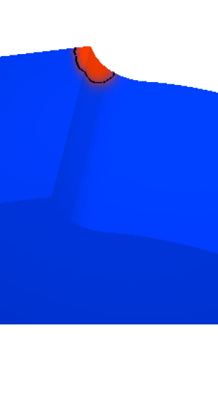
(a) $t=0.1\,$s

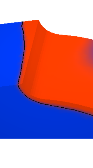
(b) $t=0.2\,$s

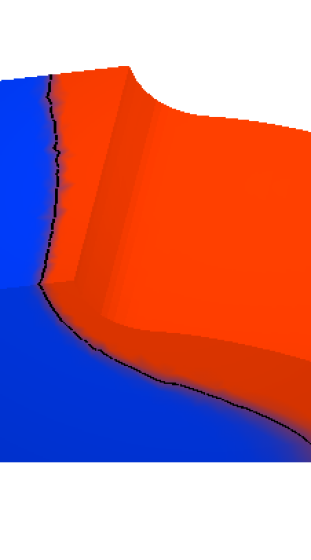
(c) $t=0.3\,$s

Figure 3: Numerical simulation of induction heating of a gear using the multifrequency approach, temperature (top row) and volume fraction of austenite (bottom row).

The heat equation also represents a parabolic equation with rapidly varying right hand side $\sigma|A_{t}|^{2}$. Since heat conduction is supposed to happen on a time scale that is much slower than the oscillating current, the temperature changes at a time scale that is much larger than that of the right hand side, which is governed by the frequency of the source current. The usual approach is to approximate the Joule heat term by its average over one period, [1]. Then, the heat equation together with the rate law describing the phase transition can be solved using time steps $\Delta t\gg\delta t$, where the rapidly varying Joule heat is replaced by an averaged Joule heat term that is obtained from the solution of the vector potential equation.

In order to reduce computational time, we make use of symmetry conditions. The cross section through the gear represents a symmetry plane, it is only necessary to consider the upper half of the geometry shown in Figure 2. In addition, it is sufficient to perform the computations only for half of a tooth. The boundary conditions on the cutting planes are adapted accordingly.

Figure 3 shows the temperature and the phase fraction of austenite for different time snapshots for a simulation using the multifrequency approach. Starting from room temperature, the temperature increases in the surface layer of the tooth and finally rises above the austenitization temperature. The formation of the high temperature phase austenite starts. After $0.3\,$s, one obtains an austenitic profile that follows the contour of the tooth. The corresponding temperature profile is shown in Figure 3 (c), the temperature is not homogeneous across the tooth, the highest temperatures are attained at the top edge of the root and at the tip of the tooth. This is an important for engineers planning a heat treatment in order to prevent a melting of the gear during the hardening process.

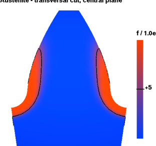
(a) MF

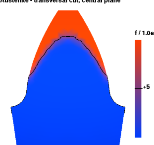
(b) HF

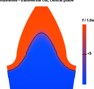
(c) MF+HF

Figure 4: Austenitic profile $z$ of a gear heated with medium-, high- and multifrequency power.

In Figure 4, simulations of the austenitic fraction using only a single frequency, either MF or HF, are compared to the multifrequency case. As one can see, in the case of MF only the root of the tooth is hardened while high frequency leads to a hardening of the tip of the tooth. Only a suitable combination of MF power, HF power and heating time leads to a contour hardening of the tooth using the multifrequency approach. The numerical computations reflect the physical aspects as explained in the introduction, see also Figure 1.

References

- [1] S. Clain, J. Rappaz, M. Swierkosz, and R. Touzani: Numerical modeling of induction heating for two-dimensional geometries, Math. Models Methods Appl. Sci., 3 (1993), 805–822.
- [2] R. Dautray, J.-L. Lions: Mathematical analysis and numerical methods for science and technology, Vol. 3, Springer, Berlin, 1990.
- [3] P.E. Druet: Higher integrability of the Lorentz force for weak solutions to Maxwell’s equations in complex geometries, WIAS preprint no. 1270, Berlin, 2007.
- [4] P.E. Druet, O. Klein, J. Sprekels, F. Tröltzsch, I. Yousept: Optimal control of three-dimensional state-constrained induction heating problems with nonlocal radiation effects. SIAM J. Control Optim. 49 (2011), 1707–1736.
- [5] G. Duvaut, J.-L. Lions: Inequalities in mechanics and physics, Springer, Berlin–New York, 1976.
- [6] J. Fuhrmann, D. Hömberg: Numerical simulation of the surface hardening of steel, Internat. J. Numer. Methods Heat Fluid Flow, 9 (1999), 705–724.
- [7] V. Girault, P.-A. Raviart: Finite element methods for Navier-Stokes equations. Theory and algorithms, Springer Series in Computational Mathematics, 5, Springer, Berlin, 1986.
- [8] M.T. González Montesinos, F. Ortegón Gallego: On an induction-conduction PDEs system in the harmonic regime, Nonlinear Analysis: Real World Applications, 15 (2014), 58-66.
- [9] R. Griesinger: The boundary value problem , vanishing at the boundary and the related decompositions of and : existence, Ann. Univ. Ferrara Sez. VII (N.S.), 36 (1990), 15–43 (1991).
- [10] D. Hömberg et. al.: Simulation of multi-frequency-induction-hardening including phase transitions and mechanical effects. In preparation.
- [11] D. Hömberg: A mathematical model for induction hardening including mechanical effects, Nonlinear Anal. Real World Appl., 5 (2004), 55–90.
- [12] D. Hömberg, J. Sokołowski: Optimal shape design of inductor coils for surface hardening, SIAM J. Control Optim., 42 (2003), 1087–1117 (electronic).
- [13] J. Kačur: Method of Rothe in evolution equations, Teubner Texts in Mathematics, 80, BSB B. G. Teubner Verlagsgesellschaft, Leipzig, 1985.
- [14] T. Kawanago: Estimation – des solutions de , C. R. Acad. Sci. Paris Sér. I Math., 317 (1993), 821–824.
- [15] J.-B. Leblond, J. Devaux: A new kinetic model for anisothermal metallurgical transformations in steels including effect of austenite grain size, Acta Metallurgica, 32 (1984), 137–146.
- [16] J. Lemaitre, J.-L. Chaboche: Mechanics of solid materials, Cambridge University Press, Cambridge, 1990.
- [17] J. C. Nédélec: Mixed finite elements in , Numer. Math., 35 (1980), 315–341.
- [18] J. Prüss: Maximal regularity for evolution equations in -spaces, Conf. Semin. Mat. Univ. Bari, 285 (2003), 1–39.
- [19] W. R. Schwenk: Simultaneous dual-frequency induction hardening, Heat Treating Progress, 3 (2003), 35–38.
- [20] J. Simon: Compact sets in the space , Ann. Mat. Pura Appl., (4) 146 (1987), 65–96.