Josephson oscillations and self-trapping of superfluid fermions
in a double-well potential

Abstract

We investigate the behaviour of a two-component Fermi superfluid in a double-well potential. We numerically solve the time dependent Bogoliubov-de Gennes equations and characterize the regimes of Josephson oscillations and self-trapping for different potential barriers and initial conditions. In the weak link limit the results agree with a two-mode model where the relative population and the phase difference between the two wells obey coupled nonlinear Josephson equations. A more complex dynamics is predicted for large amplitude oscillations and large tunneling.

I Introduction

The Josephson effect josephson ; barone is one of the key features of superconductors and superfluids. It involves very fundamental properties of these systems and has important applications. The physics of the Josephson junctions can be effectively investigated with ultracold gases confined in a double-well potential leggett ; book ; gati . The case of weakly linked Bose-Einstein condensates (BEC) has been widely studied. In the seminal papers of Smerzi et al. smerzi , coupled nonlinear Josephson equations for the relative population and the phase difference between the two wells were derived by assuming the system to be described by a superposition of left and right localized condensates (two-mode model) governed by the Gross-Pitaevskii (GP) equation (see also two-mode ). Such nonlinear Josephson equations admit solutions in the form of small periodic oscillations, whose period is determined by two key parameters: the mean-field (on-site) energy and the tunnelling energy. When the nonlinearity arising from the mean-field interaction exceeds a critical value, the system may exhibit self-trapped solutions with the relative population oscillating around a nonzero value. A large number of theoretical papers have been published along this line and experiments have also been performed gati ; florence ; oberthaler ; steinhauer ; leblanc .

Much less is known about Josephson effects in dilute Fermi gases. The Bogoliubov-de Gennes (BdG) equations for a two-component superfluid in the crossover from the Bardeen-Cooper-Schrieffer (BCS) phase to BEC were used in Ref. strinati to describe a stationary supercurrent flowing in the presence of a three-dimensional barrier with a slab geometry; the current-phase relation and the critical current were studied in the crossover for relatively low barriers, i.e., height of the barrier smaller than the chemical potential of the superfluid. The same problem was also investigated by means of a density functional approach describing bosonic Cooper pairs salasnich ; the equation of state of the gas was included via a suitable parametrization and the order parameter of the superfluid was obtained as the solution of a nonlinear Schrödinger equation (NLSE). This method gives results in good agreement with the BdG results of Ref. strinati from unitarity to the BEC limit. For a double-well potential in the weak link limit (i.e., large barriers) the same density functional can be used to derive coupled nonlinear equations for the relative population and the phase difference analog to those for BECs salasnich2 . A similar NLSE has been used to discuss in detail the transition from Josephson oscillations to self-trapping adhikari .

Some open issues are worth considering. First, the applicability of a two-mode model to weakly linked dilute Fermi superfluids has been tested so far only within a density functional approach describing a gas of bosonic pairs (namely Cooper pairs, which become molecules in the BEC limit); being a generalization of the GP equation, the theory naturally reduces to the two-mode model under the same assumptions as for coupled BECs. It is thus interesting to test the two-mode model also within a more microscopic theory like BdG which includes fermionic degrees of freedom. Second, the available BdG calculations strinati and their comparison with the density functional results salasnich are limited to the case of a stationary current through a low and thick barrier, where the flow is almost hydrodynamic and a local density approximation can be applied watanabe ; time dependent simulations with higher and thinner barriers can provide a a more stringent and informative test. Finally, the stationary BdG equations does not include bosonic collective modes (e.g., phonons) in the spectrum of excitations and cannot address the problem of dynamical instabilities, soliton nucleation, phase slips, etc., which may occur in a superfluid flow in the presence of a potential barrier. This type of physics can instead be addressed by time-dependent BdG simulations.

Motivated by the above arguments, we numerically solve the time-dependent BdG equations of a superfluid gas of fermions confined in a box with a square potential barrier at the center. The square barrier is a convenient choice for computational reasons, but the main results of this work would not change by using barriers of different shape. In the limit of weakly linked superfluids we find periodic oscillations whose frequency approaches the prediction of the two-mode model, namely the Josephson “plasma” frequency $\hbar\omega_{p}=\sqrt{E_{C}E_{J}}$ book , where the tunneling energy $E_{J}$ and the on-site mean-field energy $E_{C}$ are obtained by solving the stationary BdG equations in the same configurations. By increasing the population imbalance we explore the transition from Josephson oscillations to self-trapping. We compare the results with those obtained by solving the NLSE of Refs. salasnich ; salasnich2 ; adhikari , as well as with the predictions of the coupled nonlinear Josephson equations which can be derived from the NLSE in the weak link limit. The latter equations turn out to agree surprisingly well with the BdG simulations, provided the parameters $E_{J}$ and $E_{C}$ are consistently calculated within the same BdG theory. Finally, for large amplitude oscillations and lower barriers the dynamics is complex, involving a combination of Josephson-like oscillations, phonons and solitons.

II Bogoliubov-de Gennes equations and system configuration

We consider a three-dimensional atomic Fermi gas at zero temperature with equal populations of two spin components. The interaction between atoms in different spin states is characterized by the s-wave scattering length $a$. In experiments, this parameter can be tuned from small negative (BCS regime) to small positive (BEC regime) values by applying an external magnetic field through a Feshbach resonance. On resonance the scattering length diverges and the Fermi gas manifests universal properties (unitarity) rmp08 . We describe the gas in the BCS-BEC crossover by means of the BdG equations BdG

$$\left[\begin{array}[]{cc}\hat{H}&\Delta(r)\\ \Delta^{*}({\bf r})&-\hat{H}\end{array}\right]\left[\begin{array}[]{c}u_{\eta}({\bf r})\\ v_{\eta}({\bf r})\end{array}\right]=\varepsilon_{\eta}\left[\begin{array}[]{c}u_{\eta}({\bf r})\\ v_{\eta}({\bf r})\end{array}\right]$$ (1)

where the functions $u_{\eta}$ and $v_{\eta}$ are the fermionic quasiparticle amplitudes and $\varepsilon_{\eta}$ the corresponding quasiparticle eigenenergy; $\hat{H}=-\hbar^{2}\nabla^{2}/(2m)+V_{\rm ext}({\bf r})-\mu$ is a single-particle grand-canonical Hamiltonian for atoms of mass $m$ subject to an external potential $V_{\rm ext}$, and $\mu$ is the chemical potential. The quasiparticle amplitudes obey the normalization condition $\int d^{3}r\left[u_{\eta}^{*}({\bf r})u_{\eta^{\prime}}({\bf r})+v_{\eta}^{*}({\bf r})v_{\eta^{\prime}}({\bf r})\right]=\delta_{\eta,\eta^{\prime}}$. The order parameter of the superfluid phase is $\Delta({\bf r})=-\sum_{\eta}g_{\rm eff}({\bf r})u_{\eta}({\bf r})v_{\eta}^{*}({\bf r})$, where $g_{\rm eff}$ is a coupling constant which accounts for the interaction between atoms (see Eq. (4)); finally, the atom density is $n({\bf r})=2\sum_{\eta}\left|v_{\eta}({\bf r})\right|^{2}$. We also solve the time-dependent version of the BdG equations challis :

$$\left[\begin{array}[]{cc}\hat{H}&\Delta({\bf r},t)\\ \Delta^{*}({\bf r},t)&-\hat{H}\end{array}\right]\left[\begin{array}[]{c}u_{\eta}({\bf r},t)\\ v_{\eta}({\bf r},t)\end{array}\right]=i\hbar\frac{\partial}{\partial t}\left[\begin{array}[]{c}u_{\eta}({\bf r},t)\\ v_{\eta}({\bf r},t)\end{array}\right]\;.$$ (2)

We use an external potential $V_{\rm ext}(x)$ which depends on the longitudinal coordinate $x$ only, consisting of two hard walls placed at $x=\pm L/2$ and a rectangular barrier of height $V_{0}$ and width $d$ centered at $x=0$. The lengths $L$ and $d$ are such that the density and the order parameter of the superfluid are almost constant in the central region of each potential well on the left and right sides of the barrier. In the transverse directions the system is assumed to be uniform; in practice, we solve the equations in a transverse square box of size $L_{\perp}=13k_{F}^{-1}$ imposing periodic boundary conditions for all functions $u$ and $v$; we checked that this value of $L_{\perp}$ is large enough to make finite size effects negligible. The average density $n_{0}$ of the ground state in this potential can be used to define the Fermi wave vector of noninteracting fermions of that density, $k_{F}=(3\pi^{2}n_{0})^{1/3}$. We use $k_{F}^{-1}$ as the unit of length; we also use the corresponding Fermi energy, $E_{F}=\hbar^{2}k_{F}^{2}/(2m)$, as energy unit and $\hbar/E_{F}$ as time unit. In the calculations we can either fix the total number of atoms in the box or the density at a point at will.

The BdG equations are solved by using the same numerical method as in scott . In particular, the solution of the stationary equations (1) are found by a self-consistent iterative procedure. From the solution we can calculate the grand canonical energy $E=\langle\hat{H}-\mu\hat{N}\rangle$ of the system as

$$E=\int\!d{\bf r}\sum_{\eta}[2(\mu-\varepsilon_{\eta})|v_{\eta}({\bf r})|^{2}+\Delta^{*}({\bf r})u_{\eta}({\bf r})v_{\eta}^{*}({\bf r})]\;.$$ (3)

The time-dependent equations (2) are instead integrated by means of a $4$-th order Runge-Kutta algorithm.

The BdG equations require a regularization procedure to cure ultraviolet divergences. Here we use the method suggested in Ref. bulgac . For this, we choose a cutoff energy $E_{\rm cut}$ sufficiently far above the Fermi energy. Then, for a given external potential $V_{\rm ext}({\bf r})$ and chemical potential $\mu$, we define a local Fermi wave vector $k_{F}({\bf r})$ from the relation $\mu=\hbar^{2}k_{F}^{2}({\bf r})/(2m)+V_{\rm ext}({\bf r})$ and a cutoff wave vector $k_{\rm cut}$ from $E_{\rm cut}=\hbar^{2}k_{\rm cut}^{2}({\bf r})/(2m)+V_{\rm ext}({\bf r})-\mu$. Finally, the regularization of the interaction consists of replacing the bare coupling constant $g=4\pi\hbar^{2}a/m$, in the definition of $\Delta$ with an effective $g_{\rm eff}$ given by

$$\frac{1}{g_{\rm eff}({\bf r})}=\frac{1}{g}-\frac{mk_{\rm cut}({\bf r})}{2\pi^{2}\hbar^{2}}\left[1-\frac{k_{F}({\bf r})}{2k_{\rm cut}({\bf r})}\ln\frac{k_{\rm cut}({\bf r})+k_{F}({\bf r})}{k_{\rm cut}({\bf r})-k_{F}({\bf r})}\right]\;.$$ (4)

The cutoff energy, $E_{\rm cut}$ is chosen large enough to ensure the convergence to cutoff independent results.

III Dynamics of weakly linked Fermi superfluids at unitarity

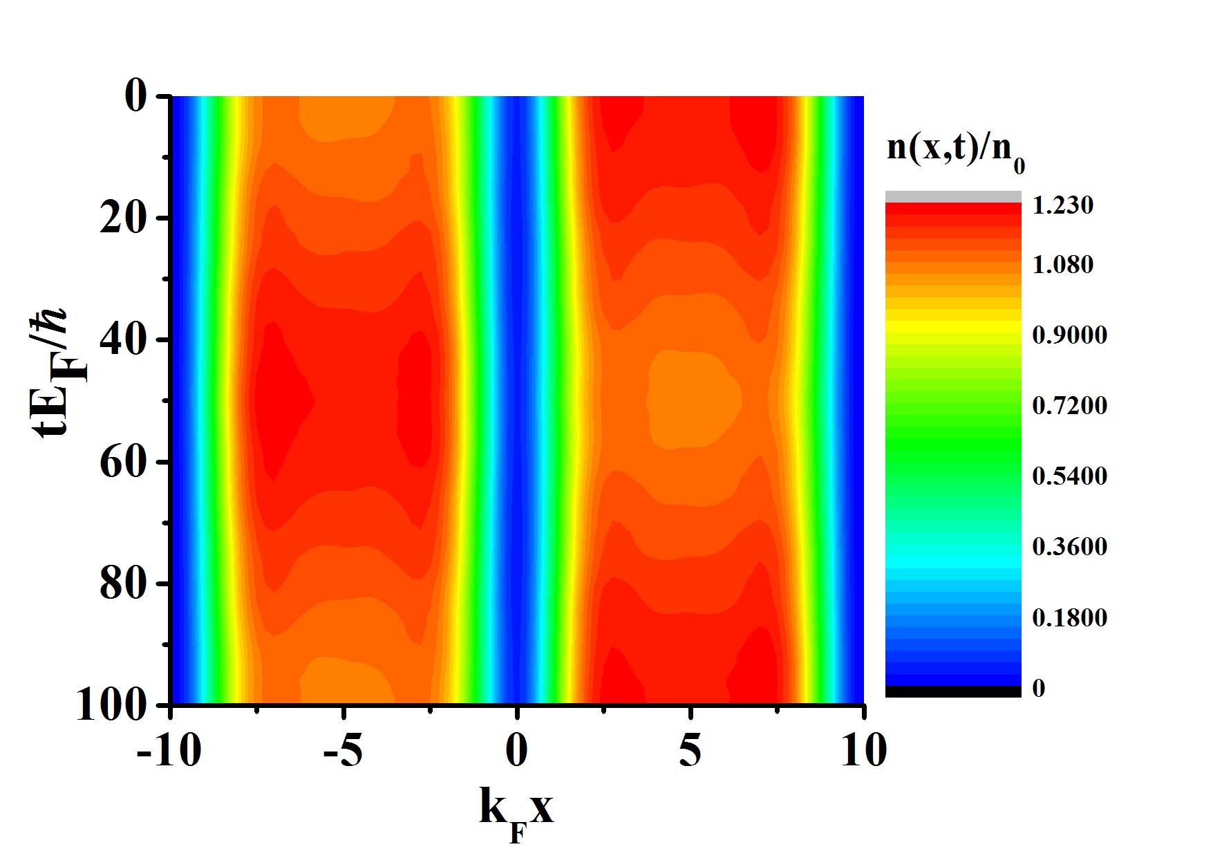
Figure 1: Evolution of the density distribution $n(x,t)/n_{0}$ of a two-component superfluid Fermi gas at unitarity and zero temperature obtained by solving the time-dependent BdG equations (2). Time, in units of $\hbar/E_{F}$, flows from top to bottom. The gas is uniform in the transverse directions and confined between hard walls in the longitudinal direction at $x=\pm L/2$ with $L=20k_{F}^{-1}$, with a central square barrier of height $V_{0}=5E_{F}$ and width $d=0.6k_{F}^{-1}$ respectively. The number of atoms is $N=100$. The initial imbalance is produced by adding a constant offset potential $V_{\rm off}$ at $t<0$ on the left side only; here we use $V_{\rm off}=0.05E_{F}$, which corresponds to an initial relative imbalance $z_{0}=(N_{L}-N_{R})/N=-0.06$. At $t=0$ the offset potential is removed and the system is let to evolve in time.

Let us consider fermions at unitarity ($1/(k_{F}a)=0$) in the presence of a thin ($d\sim k_{F}^{-1}$) and high ($V_{0}>\mu$) square barrier centered at $x=0$. We can define the number of atoms on the left, $N_{L}$, and right, $N_{R}$, as the integrals of the atom density $n(x)$ separately in the two regions of negative and positive $x$, respectively. The relative population imbalance can be defined as $z=(N_{L}-N_{R})/N$, where $N=N_{L}+N_{R}$. Another key quantity is the phase $\phi(x)$ of the complex order parameter $\Delta(x)$, which can also be different in the two wells. We define the right and left phases as $\phi_{R}=\phi(x=L/4)$ and $\phi_{L}=\phi(x=-L/4)$ respectively, and the phase difference as $\Phi=\phi_{R}-\phi_{L}$.

Our simulations start from an imbalanced configuration with $z_{0}\equiv z(t=0)\neq 0$. This is obtained by first solving the stationary BdG equations (1) with a small constant offset potential $V_{\rm off}$ on the left side of the barrier. The ground state solution in such an asymmetric potential is then used as the initial ($t=0$) state in the integration of the time-dependent BdG equations (2) in the symmetric double-well, after removing $V_{\rm off}$.

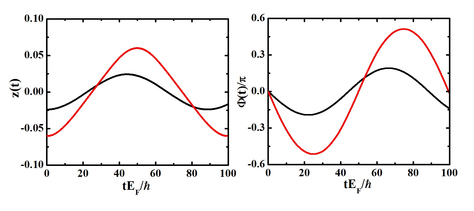
Figure 2: Relative population imbalance (left) and phase difference (right) as a function of time for the same simulation of Fig. 1 ($|z_{0}|=0.06$, red lines) and for another simulation with an even smaller initial imbalance ($|z_{0}|=0.024$, black lines).

If the initial imbalance is small ($|z_{0}|\ll 1$), the time evolution of the density and the order parameter shows clean periodic oscillations. As an example, in Fig. 1 we show the behavior of the density distribution for an initial imbalance $|z_{0}|=0.06$ and with a thin and large barrier ($d=0.6k_{F}^{-1}$ and $V_{0}=5E_{F}$). The evolution of the relative population imbalance $z(t)$ and the phase difference $\Phi(t)$ is reported in Fig. 2. The results for an even smaller imbalance are also shown in the same figure.

Josephson oscillations between weakly linked superfluids ($V_{0}\gg\mu$) are characterized by the sinusoidal relation between current and phase difference book :

$$I(t)=I_{J}\sin\Phi(t)\;,$$ (5)

where the quantity $I_{J}$ has the meaning of critical Josephson current. In our case, the current flowing at the barrier position can be easily calculated as $I=dN_{R}/dt=-dN_{L}/dt=-(N/2)dz/dt$. Fig. 3 shows four examples of the current-phase relation obtained in our simulations with different values of the initial imbalance. The upper plots correspond to the simulation of Fig. 2.

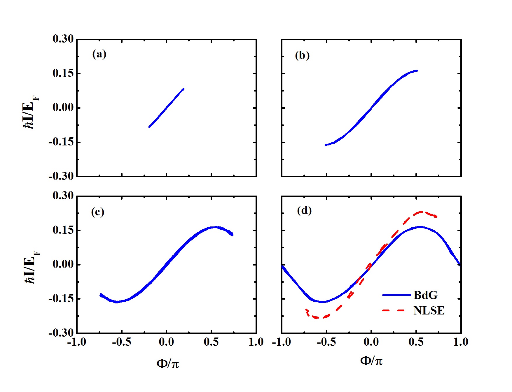
Figure 3: The current-phase relation obtained in four BdG simulations with the same barrier ($V_{0}=5E_{F}$ and $d=0.6k_{F}^{-1}$) and different initial imbalance, $z_{0}=-0.024$ (a), $-0.06$ (b), $-0.078$ (c), and $-0.096$ (d). The red dashed line in panel (d) is obtained by solving the nonlinear Schrödinger equation (10) in the same configuration and for the same initial imbalance.

If the initial imbalance exceeds a critical value, the system enters into a different dynamical regime, where one of the two wells remains always more populated than the other. The two numbers $N_{L}$ and $N_{R}$ oscillate in time, but around unequal mean values. This phenomenon is known as macroscopic quantum self-trapping smerzi . In Fig. 4 and 5 we show a typical example. The transition from the regime of Josephson oscillations and the regime of self-trapping can be visualized by plotting the trajectories in the diagram of the population imbalance vs. the phase difference. Our results for the barrier with $V_{0}=5E_{F}$ and $d=0.6k_{F}^{-1}$ are shown in Fig. 6. Josephson oscillations correspond to close trajectories, which become elliptic for small amplitudes, while self-trapping correspond to open trajectories. For the barrier used in these simulations, the transition between the two regime occurs at an initial relative imbalance $|z_{0}|\approx 0.0869$.

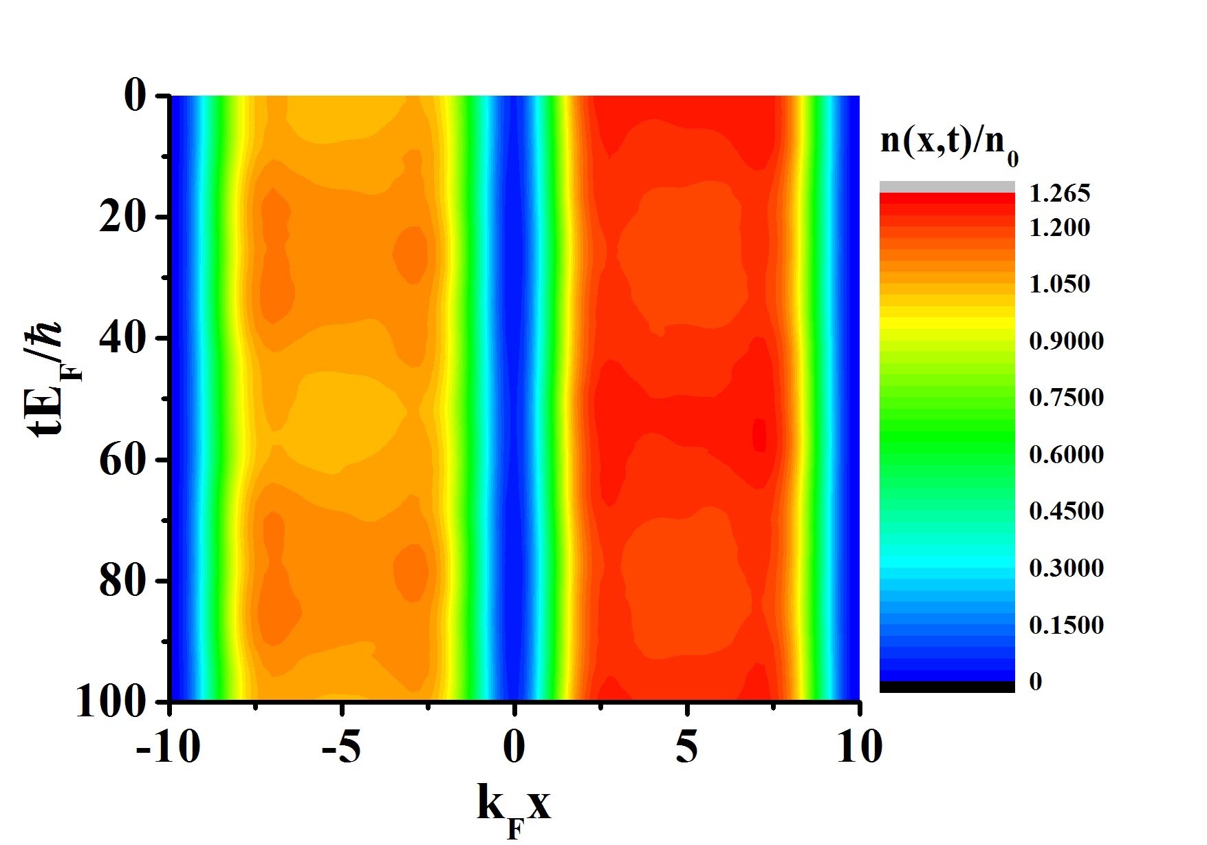
Figure 4: Same as in Fig. 1 but for a larger initial imbalance ($z_{0}=-0.096$), such to cause self-trapping.

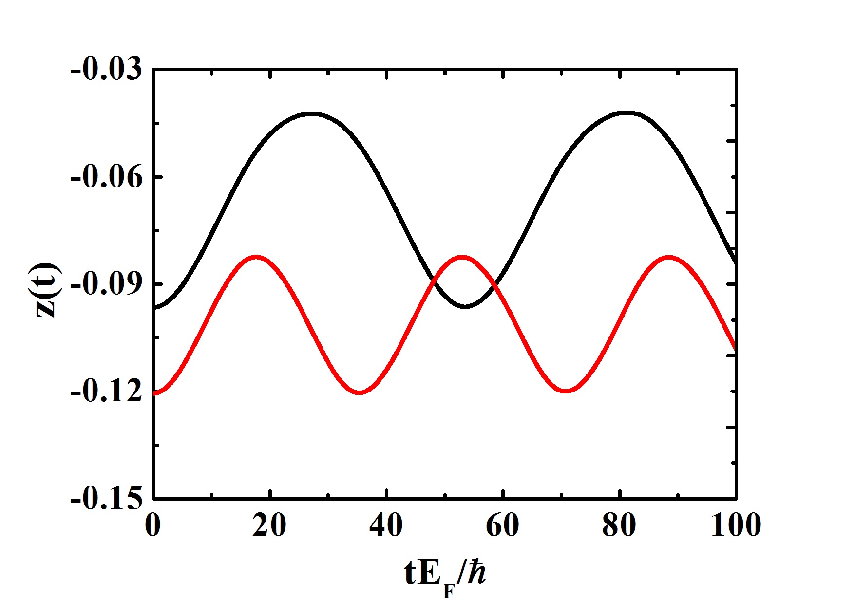
Figure 5: Relative population imbalance $z(t)$ for the same simulation of Fig. 4 ($|z_{0}|=0.096$, black line) and another simulation with an even larger initial imbalance ($|z_{0}|=0.121$, red line).

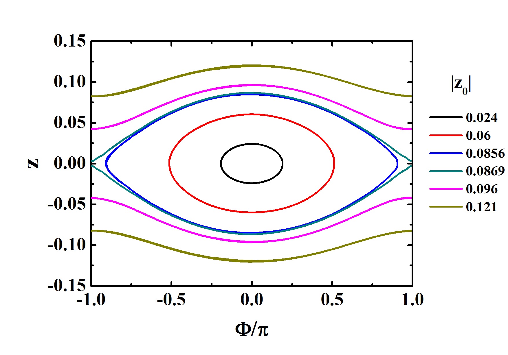
Figure 6: Population imbalance vs. phase difference in simulations with the same barrier ($V_{0}=5E_{F}$ and $d=0.6k_{F}^{-1}$) and different initial imbalance, $|z_{0}|=0.024$, $0.06$, $0.0856$, $0.0869$, $0.096$, $0.121$, from the inner ellipse to the outer open trajectory. The red ellipse corresponds to the simulation in Fig. 1; the pink open trajectory corresponds to the simulation in Fig. 4. The transition from Josephson oscillations to self-trapping occurs at about $|z_{0}|\approx 0.0869$.

IV Two-mode model for small Josephson oscillations

The purpose of this section is to show that the above BdG results for small oscillations are well reproduced by Josephson junction equations for the two dynamical variables $z(t)$ and $\Phi(t)$, provided the barrier is large enough to remain in the weak link regime. In such a situation, the system can be described as composed by two superfluids located in each well and weakly coupled by tunneling (two-mode model). Unfortunately, a rigourous derivation of the Josephson equations from the BdG equations (2) within a two-mode approximation is not available. We thus proceed by analogy with the case of bosons where, in the Josephson regime, the population imbalance and the phase difference can be seen as canonically conjugates variables entering a classical Josephson Hamiltonian of the form book

$$H_{J}=\frac{E_{C}}{2}k^{2}-E_{J}\cos\Phi\;.$$ (6)

The quantity $k$ is defined as $k=(N_{L}^{\rm(B)}-N^{\rm(B)}_{R})/2$, where $N_{L}^{\rm(B)}$ and $N^{\rm(B)}$ are the number of bosons on the left and right side of the barrrier, and is assumed to be small. The quantities $E_{C}$ and $E_{J}$ have the meaning of on-site energy (local interaction within each well) and tunneling energy (or Josephson coupling energy), respectively. From (6) one gets the equations of motion

$$\frac{\partial k}{\partial t} = -\frac{\partial H_{J}}{\partial(\hbar\Phi)}=-\frac{E_{J}}{\hbar}\sin\Phi$$ (7)

$$\frac{\partial\Phi}{\partial t} = \frac{\partial H_{J}}{\partial(\hbar k)}=\frac{E_{C}}{\hbar}k\;.$$ (8)

If $|\Phi|\ll 1$, the two equations admit harmonic solutions corresponding to Josephson oscillations of frequency

$$\omega_{p}=\frac{1}{\hbar}\sqrt{E_{C}E_{J}}$$ (9)

also known as plasma frequency. These results are valid in the Josephson regime where $E_{C}/E_{J}$ is of order $1$ or less, but much larger than $N^{-2}$; different regimes are obtained when $E_{C}/E_{J}\ll N^{-2}$ (Rabi regime) and $E_{C}/E_{J}\gg 1$ (Fock regime) leggett ; gati ; smerzi .

In order to check the applicability of this scheme to the BdG results of the previous section, we need to know how to calculate $E_{C}$ and $E_{J}$ within the same theory. We first notice that the tunneling energy $E_{J}$ can be easily related to the energy difference $\Delta E=E^{-}-E^{+}$, where $E^{+}$ and $E^{-}$ are the energies of the lowest symmetric and antisymmetric states in the double-well potential with zero imbalance ($k=0$). In fact, these states have $\Phi=0$ and $\Phi=\pi$, respectively, and hence the Hamiltonian (6) gives $E_{J}=\Delta E/2$. Moreover we can relate both $E_{J}$ and $\Delta E$ to the Josephson current $I_{J}$. In fact, the number of bosons, i.e., pairs of fermionic atoms, tunneling through the barrier at $x=0$ per unit time is $I^{\rm(B)}=-dk/dt$, so that the current of atoms is $I=2I^{\rm(B)}=(2E_{J}/\hbar)\sin\Phi$, as in Eq. (5), with $I_{J}=2E_{J}/\hbar=\Delta E/\hbar$.

A nice feature of the last relation is that it can be numerically tested by performing two independent calculations. On one hand, the Josephson current $I_{J}$ can be obtained by solving the time dependent BdG equations (2): by looking at the current-phase plots, like those in Fig. 3, the current $I_{J}$ can be extracted as the maximum of the curve. On the other hand, the energy difference $\Delta E$ can be calculated by solving the stationary BdG equations (1) for the ground (symmetric) state and the lowest antisymmetric state (see details in the Appendix). In Fig. 7 we show the results obtained with $100$ particles in a box of size $L=20k_{F}^{-1}$ and different barriers. The figure shows that the relation $I_{J}=\Delta E/\hbar$ is remarkably well satisfied.

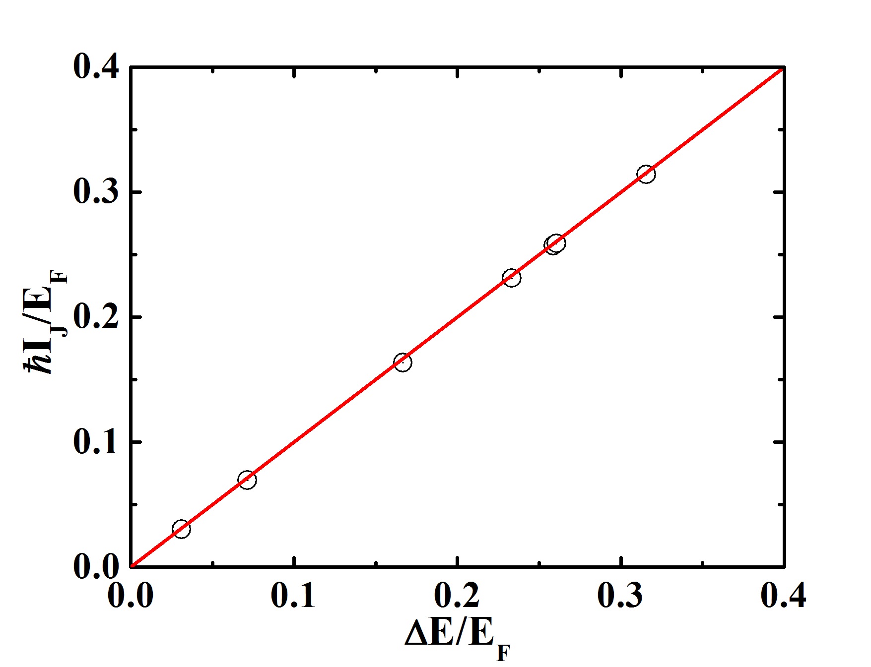
Figure 7: The Josephson current $I_{J}$ extracted from time dependent BdG simulations in the regime of small oscillations and weak tunneling is plotted as a function of the energy difference $\Delta E=E^{-}-E^{+}$, between the lowest antisymmetric and symmetric solutions of the stationary BdG equations (1). All points correspond to $E_{\rm cut}=50E_{F}$, $N=100$, $L=20k_{F}^{-1}$ and $L_{\perp}=13k_{F}^{-1}$, while ($V_{0}/E_{F}$, $k_{F}d$) is (5,1), (5,0.8), (5,0.6), (6,0.45), (5,0.5), (4,0.6), (4,0.55), for points from bottom-left to top-right. The red line represents the equality $\hbar I_{J}=\Delta E$.

The on-site energy $E_{C}$ accounts for the variation of the interaction energy of the system due to the exchange of particles between the two wells. For a bosonic superfuid in a symmetric well, this parameter is given $E_{C}=2d\mu^{\rm(B)}/dN_{L}^{\rm(B)}$ book , where $\mu^{\rm(B)}$ is the chemical potential and its derivative is calculated at $N_{L}^{\rm(B)}=N^{\rm(B)}/2$. Expressing the same quantity in terms of the chemical potential of the fermionic atoms and the number of atoms, we can write $E_{C}=8d\mu/dN_{L}$. This quantity can be obtained by solving the stationary BdG equations (1) for different atom numbers in the same double-well. Having $E_{J}$ and $E_{C}$, we can finally calculate the plasma period $T_{p}=2\pi/\omega_{p}=h/\sqrt{E_{C}E_{J}}$ and compare it with the period of the oscillations observed in the time-dependent BdG simulations. The comparison is reported in Fig. 8, where we plot $T_{\rm BdG}$ (black solid line) and $T_{p}$ (red dashed line) as a function of $E_{J}=\Delta E/2$. As one can see, in the limit of small tunneling ($\Delta E\to 0$), the period observed in the BdG simulations nicely approach the plasma period $T_{p}$.

These results show that the small oscillations of two weakly coupled fermionic superfluids at unitarity, as obtained with the BdG equations, can be accurately reproduced by a two-mode model for Josephson oscillations.

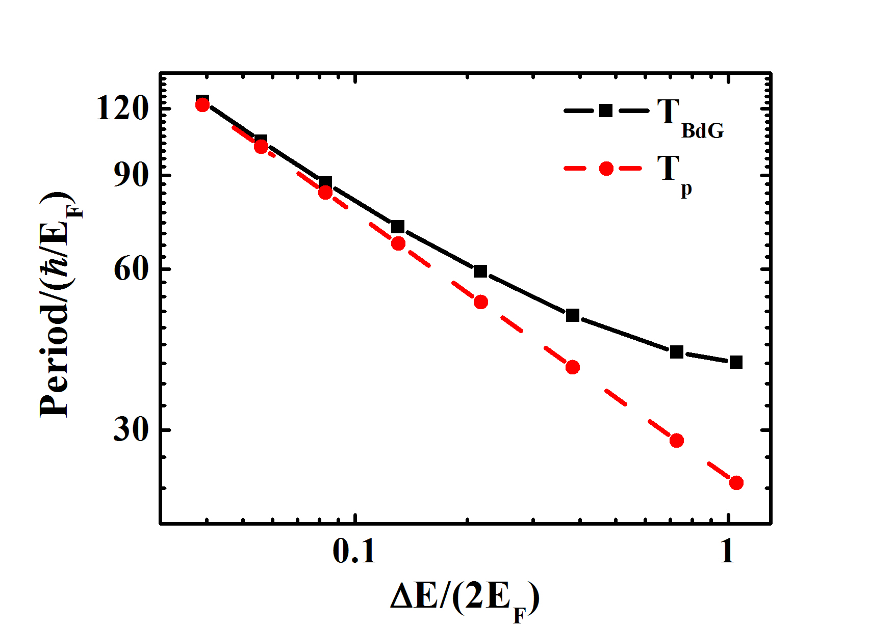
Figure 8: Period of small amplitude Josephson oscillations as a function of $\Delta E/2$, in log-log scale. The black solid line is the period $T_{BdG}$ observed in time dependent BdG simulations for $100$ atoms in a double-well potential. For each black point the width of the barrier is the same, $d=0.6k_{F}^{-1}$, while its height decreases from $V_{0}=7E_{F}$ (leftmost point) to $0.6E_{F}$ (rightmost point). The red dashed line is the period $T_{p}=2\pi/\omega_{p}=h/\sqrt{E_{C}E_{J}}$ of plasma oscillations, where $E_{C}$ and $E_{J}$ are calculated by solving the stationary BdG equations (1), assuming $E_{J}=\Delta E/2$.

V Large oscillations and self-trapping

Let us now consider larger oscillations and the transition to self-trapping. The classical Josephson Hamiltonian (6) does not apply anymore and we may wonder whether nonlinear effects can be properly included in a two-mode model. For Bose-Einstein condensates governed by the Gross-Pitaevskii equation, coupled nonlinear Josephson junction equations for the number imbalance and the phase were analytically derived by Smerzi et al. smerzi . A similar derivation is also available for fermions in the BCS-BEC crossover within a phenomenological density functional theory salasnich2 . This theory is based on the use of the following nonlinear Schrödinger equation (also named density functional GP equation, or extended Thomas-Fermi equation)

$$i\hbar\frac{\partial}{\partial t}\Psi({\bf r},t)=[-\frac{\hbar^{2}}{4m}\nabla^{2}+2V_{ext}({\bf r})+\mu_{\rm loc}^{(B)}(n,a)]\Psi({\bf r},t)$$ (10)

for the order parameter $\Psi$ of Cooper pairs of mass $2m$, with $|\Psi({\bf r})|^{2}=n({\bf r})/2$, if $n$ is the atom density. The key ingredient of this nonlinear Schrödinger equation is the local "bulk" chemical potential of Cooper pairs, $\mu_{\rm loc}^{(B)}(n,a)=2\mu(n,a)+\hbar^{2}/(ma^{2})$, where $\mu(n,a)$ is the chemical potential of a uniform Fermi gas of density $n$ and the second term is the binding energy of the pair. Its expression is an input of the theory; it can be taken from ab initio Monte Carlo calculations of the equation of state or from the mean-field BdG theory, or different suitable parametrizations. Once $\mu_{\rm loc}(n,a)$ is given, the NLSE (10) can be numerically solved for studying stationary and/or time dependent configurations. The advantages and the limits of this approach have been widely discussed in the literature (see for instance the recent discussion in forbes , and references therein). Here we only focus on the fact that, when applied to a double-well potential in the weak link limit, the NLSE can be cast into the form of Josephson junction equations salasnich2 . This is done by assuming the order parameter to be a superposition of the left and right parts,

$$\Psi({\bf r},t)=c_{L}(t)\Psi_{L}({\bf r})+c_{R}(t)\Psi_{R}({\bf r})$$ (11)

having an exponentially small overlap under the central barrier. By inserting this ansatz for $\Psi$ into Eq. (10), after integration over space and neglecting exponentially small $\Psi_{L}\Psi_{R}$ terms, one obtains the equations

$$i\hbar\frac{\partial}{\partial t}c_{L}(t) = E_{L}c_{L}(t)-{\cal K}c_{R}(t)$$ (12)

$$i\hbar\frac{\partial}{\partial t}c_{R}(t) = E_{R}c_{R}(t)-{\cal K}c_{L}(t)$$ (13)

for the two complex coefficients $c_{i}(t)$ in region $i$, with $i=L,R$. The energy $E_{i}=E_{i}^{0}+E_{i}^{I}$ is the sum of

$$E^{0}_{i}(\sqrt{N_{i}})=\int d{\bf r}\Psi_{i}({\bf r})[-\frac{\hbar^{2}}{4m}\nabla^{2}+2V_{\rm ext}({\bf r})]\Psi_{i}({\bf r})$$ (14)

$$E^{I}_{i}(\sqrt{N_{i}})=\int d{\bf r}\Psi_{i}({\bf r})\mu^{(B)}_{\rm loc}(n_{i},a)\Psi_{i}({\bf r})\;,$$ (15)

while the coupling term is given by

$${\cal K}=-\int d{\bf r}\Psi_{L}({\bf r})[-\frac{\hbar^{2}}{4m}\nabla^{2}+2V_{\rm ext}({\bf r})]\Psi_{R}({\bf r})\;.$$ (16)

The functions $\Psi_{R}(\textbf{r})$ and $\Psi_{L}(\textbf{r})$ are real, obey the orthonormality condition $\int d\textbf{r}\Psi_{i}\Psi_{j}=\delta_{i,j}$ and are localized in each of the two wells. In a symmetric system (i.e., $V_{\rm ext}(-\rm\textbf{r})=V_{\rm ext}(\rm\textbf{r})$), one has $\Psi_{R}(-\textbf{r})=\Psi_{L}(\textbf{r})$ and thus $E_{L}^{0}=E_{R}^{0}$ and $E_{L}^{I}=E_{R}^{I}=E^{I}$. By writing $c_{L,R}=\sqrt{N_{L,R}/2}\exp(i\phi_{L,R})$ and inserting it into Eqs. (12) and (13), one gets salasnich2

$$\frac{\partial z}{\partial t} = -\frac{2{\cal K}}{\hbar}\sqrt{1-z^{2}}\sin\Phi$$ (17)

$$\frac{\partial\Phi}{\partial t} = \frac{1}{\hbar}[E^{I}(\sqrt{N_{L}})-E^{I}(\sqrt{N_{R}})]+\frac{2{\cal K}}{\hbar}\frac{z\cos\Phi}{\sqrt{1-z^{2}}}$$ (18)

where the imbalance $z$ and the phase difference $\Phi$ are the same already defined at the beginning of section III.

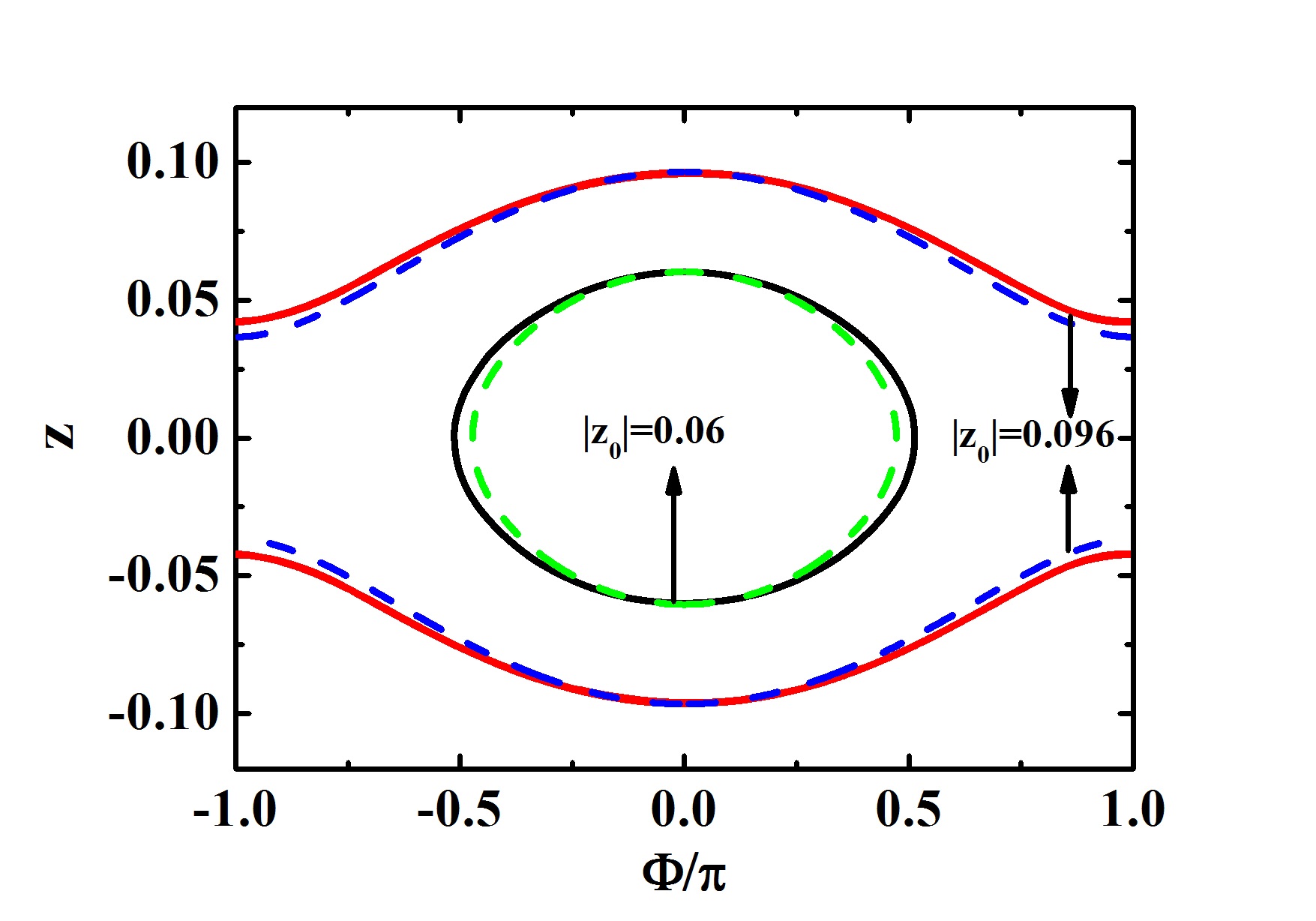
Figure 9: Population imbalance vs. phase difference. The potential barrier has height $V_{0}=5E_{F}$ and width $d=0.6k_{F}^{-1}$, as in Fig. 6. Solid lines are the results of time-dependent BdG simulations, while dashed lines are the solutions of the nonlinear Josephson equations (17) and (19), with $E_{J}=0.0833E_{F}$ and $E_{C}=0.0678E_{F}$ taken from the solutions of the stationary BdG equations. Closed trajectories correspond to Josephson oscillations with initial imbalance $|z_{0}|=0.06$, while open trajectories correspond to self-trapped states with $|z_{0}|=0.096$.

At unitarity the chemical potential of the uniform Fermi gas of density $n$ is $\mu(n)=(1+\beta)E_{F}(n)$, where $\beta$ is a universal parameter rmp08 . This implies $E^{I}(\sqrt{N_{i}})=U(N_{i}/2)^{2/3}$ with $U=[\hbar^{2}(3\pi^{2})^{2/3}(1+\beta)/m]\int\!d{\bf r}\Psi_{i}^{10/3}$, and Eq. (18) becomes

$$\frac{\partial\Phi}{\partial t}=\frac{2{\cal K}}{\hbar}\left(\Lambda[(1+z)^{2/3}-(1-z)^{2/3}]+\frac{z\cos\Phi}{\sqrt{1-z^{2}}}\right)$$ (19)

where $\Lambda=(N/4)^{2/3}U/2{\cal K}$ adhikari ; noteN . The corresponding classical Hamiltonian is

$$\frac{H}{2{\cal K}}=\frac{3\Lambda}{5}[(1+z)^{5/3}+(1-z)^{5/3}]-\sqrt{1-z^{2}}\cos\Phi\;.$$ (20)

In the limit of small amplitude oscillations ($|\Phi|\ll 1$ and $|z|\ll 1$), the equations of motion (17) and (19) reduce to the linear Josephson equations (7) and (8) provided the two parameters $\Lambda$ and ${\cal K}$ are related to the on-site interaction energy $E_{C}$ and the tunneling energy $E_{J}$ by

$${\cal K}=\frac{2E_{J}}{N}\;,\;\Lambda=\frac{3}{4}\left(\frac{N^{2}E_{c}}{16E_{J}}-1\right)\;.$$ (21)

At this point we are ready to compare our BdG results of section III with the two-mode model including the nonlinear regime. For each configuration (i.e., for each set of parameters $L,L_{\perp},V_{0},d,N$) we can calculate the two energies $E_{C}$ and $E_{J}$ by solving the stationary BdG equations as explained in section IV. Then we can use them in (21) to calculate ${\cal K}$ and $\Lambda$ and solve the nonlinear Josephson equations (17) and (19) for different values of the initial population imbalance. The results can then be compared with those obtained by solving the time dependent BdG equations (2). In Fig. 9 we show typical results for the imbalance vs. phase diagram, for the same configuration of Fig. 6. The agreement between BdG equations (solid lines) and nonlinear Josephson equations (dashed lines) is remarkably good both in the case of Josephson oscillations (inner ellipse) and self-trapping (open trajectories). In the BdG simulations the transition between the two regimes occurs at $|z_{0}|\approx 0.0869$. In the case of the nonlinear Josephson equations (17) and (19) the same transition is obtained when the energy (20) reaches the critical value adhikari

$$E_{\rm cr}=2{\cal K}\left(\frac{6\Lambda}{5}+1\right)=\frac{4E_{J}}{N}\left(\frac{9N^{2}E_{C}}{160E_{J}}+\frac{1}{10}\right)\;.$$ (22)

For the parameters of Fig. 9, this condition corresponds to $|z_{0}|\approx 0.0893$, which is again very close to the BdG result.

The agreement between BdG equations and nonlinear Josephson equations is not restricted to unitarity. We tested that a similar agreement is found also for $1/(k_{F}a)\neq 0$, both at the BEC side ($1/(k_{F}a)>0$) and BCS side ($1/(k_{F}a)<0$) of the BCS-BEC crossover. This suggests that the validity of the nonlinear Josephson equations (17) and (18) is more general than the validity of the NLSE (10) which is known to be accurate in the BEC regime but not in the BCS regime, where it misses the fermionic degrees of freedom. In Ref. salasnich2 it was noticed that, despite this inaccuracy of the NLSE, the nonlinear Josephson equations can still be used in the whole crossover, provided the tunnelling energy is taken as a phenomenological parameter. Our numerical results show that the same nonlinear Josephson equations are a very good approximation of the weak link limit of the BdG equations, the parameters $E_{C}$ and $E_{J}$ being consistently calculated within the same BdG theory.

The difference between NLSE and BdG equations can be appreciated by looking at Fig. 10, where we plot the results for the maximum Josephson current, $I_{J}$, together with the energy difference $\Delta E$. The quantity $I_{J}$ is extracted from time dependent simulations, either solving the BdG equations (2) (red solid line) or the NLSE (10) (upper dashed line), while $\Delta E$ is calculated from the corresponding stationary (time independent) equations; in Eq. (10) we use the mean-field equation of state (MF EOS) for the local chemical potential salasnich2 . As discussed in section IV, in the weak link limit, where the nonlinear Josephson equations are expected to hold, the quantity $\Delta E$ should be equal to twice the tunneling energy $E_{J}$ and one should find $\hbar I_{J}=\Delta E$. This is clearly the case for BdG equations where $\Delta E$ (black solid line) and $\hbar I_{J}$ (red solid line) are almost indistinguishable in the whole crossover, the small difference in the BEC limit being likely due to the finite cutoff energy in the BdG calculations, which becomes a more critical parameter as $1/(k_{F}a)$ increases. Conversely in the case of NLSE, the two quantity are significantly different and the critical current $I_{J}$ is increasingly larger than the BdG prediction in the BCS limit. The difference can be seen also in Fig. 3 where we show an example of Josephson oscillations at unitarity as obtained by solving Eq. (10) (dashed line) and Eq. (2) (solid line) for the same configuration. The fact that $I_{J}$ is larger in the NLSE than in BdG equations is well known and is simply due to pair-breaking processes which are included in BdG combescot but are absent in the NLSE. This effect was already discussed in Ref. salasnich2 in a regime of wider ($d>k_{F}^{-1}$) and lower ($V_{0}<E_{F}$) barriers. Here, on purpose, we have chosen thinner barriers, i.e, $d$ of the order or less than $k_{F}^{-1}$, in order to test the applicability of the two-mode model to cases where density and phase variations occur on the lengthscale of the inverse Fermi wave vector, such that the local density approximation becomes questionable and fermionic degrees of freedom might play a role. Our results indicate that, at least in the weak link limit and within a mean-field theory, the dynamics is still dominated by tunneling of bosonic pairs and is suprisingly well described by the nonlinear Josephson equations (17)-(18).

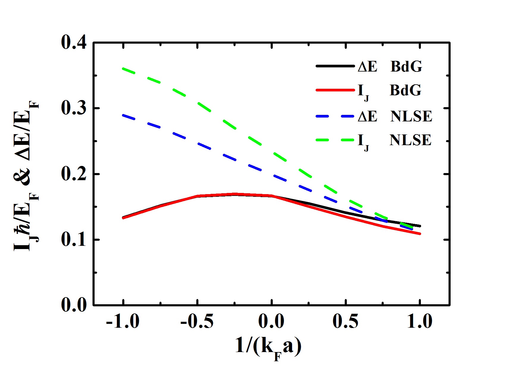
Figure 10: Energy difference $\Delta E$ and maximum Josephson current $I_{J}$ calculated with the BdG equations (solid lines) and the NLSE (dashed lines), as a function of the interaction strength $1/(k_{F}a)$. The parameters of the barrier are $d=0.6k_{F}^{-1}$ and $V_{0}=5E_{F}$, and the number of atoms $N=100$.

The situation is rather different when the coupling between the two wells is strong. An example is shown in Fig. 11, where we plot the density $n(x,t)$ in a BdG simulation with a low barrier ($V_{0}=E_{F}$ and $d=0.6k_{F}^{-1}$) and large initial imbalance. The Josephson current through the barrier is strongly coupled to the collective motion of the gas in the two wells. One can distinguish a density wave bouncing back and forth with a velocity of the order of the sound speed in a unitary Fermi gas with the same average density, $\sqrt{(1+\beta)/3}\ v_{F}$rmp08 . In addition, at about $t=15\hbar/E_{F}$, when the density under the barrier almost vanishes, a grey soliton is nucleated. The soliton appears as a density depletion travelling leftward (dashed line) at a velocity smaller than the speed of sound. The phase of the order parameter has a variation of the order of $\pi$ across the soliton. In the case of an infinite system, this mechanism of soliton nucleation induces a dissipation of the superfluid current due to phase slip piazza . In our confined double-well system, solitons and collective sound-like waves are coupled by nonlinear mixing and eventually lead to a decay of the initial Josephson oscillation.

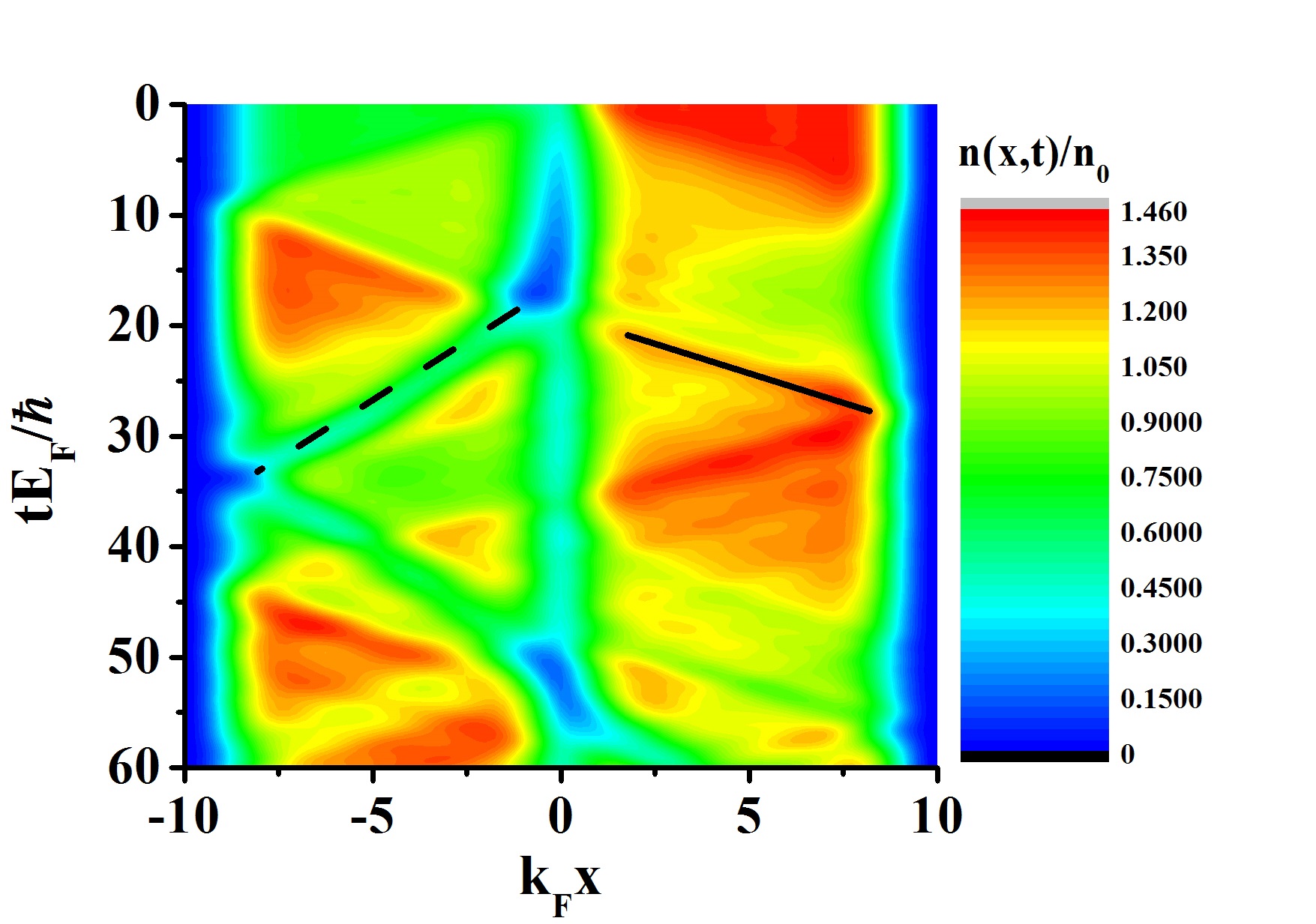
Figure 11: Evolution of the density distribution $n(x,t)/n_{0}$ at unitarity, obtained by solving the time-dependent BdG equations (2), as in Fig. 1, but for a lower barrier ($V_{0}=E_{F}$ and $d=0.6k_{F}^{-1}$). The initial imbalance is $|z_{0}|=0.353$. Solid and dashed lines represent the propagation of a sound-like density wave packet and a grey soliton, respectively.

VI Conclusions

Two weakly linked Fermi superfluids in a double well geometry exhibit dynamical regimes of Josephson oscillations and self-trapping. The nonlinear Josephson equations that describe both regimes are the analog of those for Bose superfluids described by the GP equation smerzi ; indeed the fermionic versions of such equations were previously derived starting from a generalized GP equation salasnich2 . Here we show that the same nonlinear Josephson equations are in remarkable agreement with time-dependent BdG simulations, with the on-site energy, $E_{C}$, and the tunneling energy, $E_{J}$, consistently calculated within the same BdG theory. Such an agreement could not be foretold a priori since, on one hand, a formal derivation of the nonlinear Josephson equations from the BdG equations is yet missing and, on the other hand, the role played by fermionic degrees of freedom in the dynamics of a superfluid subject to density and phase variations on the lengthscale of the inverse Fermi wave vector is largely unkown. Our results indicate that the dynamics at the weak link is dominated by tunneling of bosonic pairs, with the caveat that the critical Josephson current $I_{J}$ in the BCS side of the crossover is determined by pair-beaking processes. For lower barriers and large tunneling, the dynamics involves the collective motion of the superfluid in the two wells and possible phase slip processes due to the nucleation of solitons. Our predictions complement those of Ref. strinati and are intended to stimulate new experimental investigations with ultracold Fermi gases in double-well potentials.

Appendix: Calculation of the energy difference $\Delta E$

In this appendix we provide some details about the calculations of the energy difference, $\Delta E=E^{-}-E^{+}$, where $E^{+}$ is the energy of the (symmetric) ground state of the gas and $E^{-}$ is the energy of the lowest anti-symmetric state with the same number of particles $N$ in the box. Here symmetric and anti-symmetric refer to spatial reflection in the $x$-direction around $x=0k_{F}^{-1}$. The anti-symmetric state corresponds to the solutions of Eq. (1) exhibiting a $\pi$ phase jump in the order parameter $\Delta$ when crossing the center of the box. For weakly coupled superfluids the quantity $\Delta E$ is directly related to the Josephson tunnelling energy, $E_{J}$ as already seen in section IV.

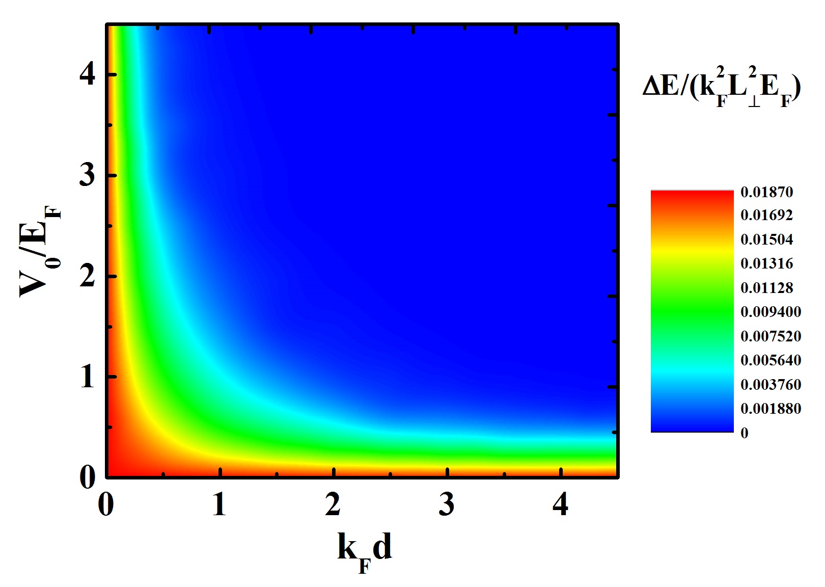
Figure 12: Energy difference $\Delta E=E^{-}-E^{+}$, divided by the area $L_{\perp}^{2}$, as a function of the barrier height $V_{0}$ and width $d$. Here $N=156$, $L_{\perp}=13k_{F}^{-1}$, $L=30k_{F}^{-1}$, and $E_{\rm cut}=70E_{F}$.

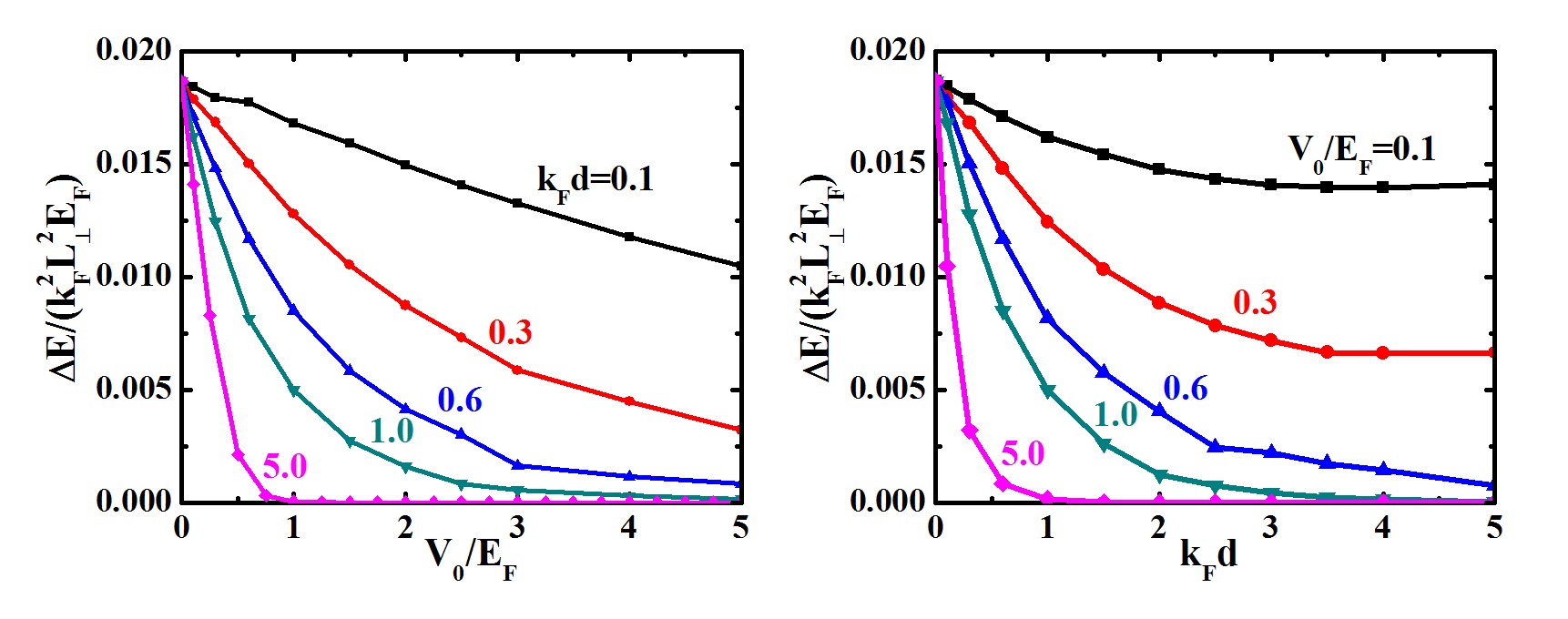
Figure 13: Left: energy difference $\Delta E=E^{-}-E^{+}$, divided by the area $L_{\perp}^{2}$, as a function of the barrier height $V_{0}$ for different widths $d$. Right: the same quantity as a function of the barrier width $d$ for different values of height $V_{0}$. All the other parameters are the same as in the previous figure.

Since the quantity $\Delta E$ is typically much smaller than the energies $E^{-}$ and $E^{+}$, we must take care of all possible sources of numerical inaccuracy, in particular those introduced by the finite cutoff energy and the finite box. We have first checked that, at unitarity, without barrier and in the limit of large $L$, the energy $E^{+}$ converges to the energy of a uniform infinite gas: $(E^{+}/N)=(3/5)\mu=(3/5)(1+\beta)E_{F}=0.354E_{F}$, where $\beta=-0.41$ is the value of the Bertsch parameter in BdG theory rmp08 . In the same situation, the quantity $\Delta E$ measures the cost in energy associated to creation of the density depletion and the nodal structure of the order parameter at the box center, corresponding to a dark soliton antezza . The energy per unit surface of a planar dark soliton at unitarity is $\epsilon_{s}=\Delta E/(E_{F}k_{F}^{2}L_{\perp}^{2})$ and BdG theory gives $\epsilon_{s}=(1+\beta)^{1/2}/(8\pi\sqrt{3})\simeq 0.0176$ brand . We have checked that both analytic values are reproduced within an accuracy of about $2$%, which is enough for our purposes.

Our results for $\Delta E$ as a function of $V_{0}$ and $d$ are shown in Figs. 12 and 13. All results in these figures are obtained by using $N=156$, $L_{\perp}=13k_{F}^{-1}$, $L=30k_{F}^{-1}$, and $E_{\rm cut}=70E_{F}$. As expected, $\Delta E$ approaches the same value in the limit of vanishingly small barrier (i.e, for $V_{0}\to 0$ at finite $d$). This value is $\Delta E/(k_{F}^{2}L_{\perp}^{2}E_{F})\simeq 0.0185$, which is slightly larger than the energy of dark soliton in an infinite system, due to the finite box sixe. For $d$ of the order of $k_{F}^{-1}$, the quantity $\Delta E$ is rapidly decreasing when $V_{0}$ increases. The case of large barriers and small tunnelling (weak link) is where the physics of the Josephson effect is expected to manifest.

Finally we note that for $V_{0}$ much smaller than $E_{F}$ the quantity $\Delta E$ tends to be a constant value when $d\to\infty$. A simple explanation of this behavior is obtained by considering that, for a very wide and low barrier, the effect of the barrier is that of lowering the “bulk” density in the central region of the box. If $d$ is larger that the soliton width, which is of the order of a few $k_{F}^{-1}$, this effect can be accounted for by calculating the energy of a dark soliton in uniform gas of reduced density. Further increasing the width of the barrier has no effects on the soliton energy and hence $\Delta E$ remains constant.

References

- (1) B. D. Josephson, Phys. Lett. 1, 251 (1962).
- (2) A. Barone and G. Paterno, Physics and Applications of the Josephson Effect (Wiley, New York, 1982).
- (3) A.J.Leggett, Rev. Mod. Phys. 73, 307 (2001).
- (4) L.Pitaevskii and S.Stringari, Bose-Einstein Condensation (Oxford Science Publications, 2003).
- (5) R.Gati and M.K.Oberthaler, J. Phys. B: At. Mol. Opt. Phys. 40, R61 (2007).
- (6) A. Smerzi, S. Fantoni, S. Giovanazzi, and S.R.Shenoy, Phys. Rev. Lett. 79, 4950 (1997); S.Raghavan, A.Smerzi, S.Fantoni, and S.R.Shenoy, Phys. Rev. A 59, 620 (1999).
- (7) E.A. Ostrovskaya, Y. S. Kivshar, M. Lisak, B. Hall, F. Cattani, and D. Anderson, Phys. Rev. A 61, 031601R (2000); D. Ananikian and T. Bergeman, Phys. Rev. A 73, 013604 (2006).
- (8) F.S.Cataliotti, S. Burger, C. Fort, P. Maddaloni, F. Minardi, A. Trombettoni, A. Smerzi, and M. Inguscio, Science 293, 843 (2001).
- (9) Th.Anker, M.Albiez, R.Gati, S.Hunsmann, B.Eiermann, A.Trombettoni, and M.K.Oberthaler, Phys. Rev. Lett. 94, 020403 (2005); M.Albiez, R.Gati, J.Foelling, S.Hunsmann, M.Cristiani, M.K.Oberthaler, Phys. Rev. Lett. 95, 010402 (2005); T.Zibold, E.Nicklas, Ch.Gross, and M.K.Oberthaler, Phys. Rev. Lett. 105, 204101 (2010).
- (10) S. Levy, E. Lahoud, I. Shomroni, and J. Steinhauer, Nature 449, 579 (2007).
- (11) L. J. LeBlanc, A. B. Bardon, J. McKeever, M. H. T. Extavour, D. Jervis, J. H. Thywissen, F. Piazza, A. Smerzi, Phys. Rev. Lett. 106, 025302 (2011).
- (12) P. Pieri and G. C. Strinati, Phys. Rev. Lett. 91, 030401(2003).
- (13) A. Spuntarelli, P. Pieri, and G. C. Strinati, Phys. Rev. Lett. 99, 040401(2007), and Phys. Reports 488, 111 (2010).
- (14) F.Ancilotto, L.Salasnich, F.Toigo, Phys. Rev. A 79, 033627 (2009).
- (15) L.Salasnich, N.Manini, F.Toigo, Phys. Rev. A 77, 043609 (2008); L. Salasnich, F. Ancilotto, N. Manini, F. Toigo, Laser Phys. 19, 636 (2009).
- (16) S. K. Adhikari, Hong Lu, and Han Pu, Phys. Rev. A 80, 063607 (2009).
- (17) G.Watanabe, F. Dalfovo, F. Piazza, L. P. Pitaevskii, S. Stringari, Phys. Rev. A 80, 053602 (2009).
- (18) S.Giorgini, L.Pitaevskii, S.Stringari, Rev. Mod. Phys. 80, 1215 (2008).
- (19) P.G. de Gennes, Superconductivity of Metals and Alloys, (Benjamin, new York, 1966); A.J. Leggett, in Modern Trends in the Theory of Condensed Matter, edited by A. Pekalski and R. Przystawa (Springer-Verlag, Berlin, 1980); M. Randeria, in Bose Einstein Condensation, edited by A. Griffin, D. Snoke, and S. Stringari (Cambridge, Cambridge, England,1995).
- (20) K. J. Challis, R. J. Ballagh, and C.W. Gardiner, Phys. Rev. Lett. 98, 093002 (2007).
- (21) R. G. Scott, F. Dalfovo, L. P. Pitaevskii, and S. Stringari, Phys. Rev. Lett. 106, 185301(2011).
- (22) Aurel Bulgac and Yongle Yu, Phys. Rev. Lett. 88, 042504(2002).
- (23) M. McNeil Forbes and R. Sharma, arXiv:1308.4387.
- (24) Here the notation is the same as in Ref.adhikari except for the meaning of which, in the present work, is the number of fermionic atoms, while in adhikari is the number of bosonic dimers. In the context of NLSE the two numbers differ only by a factor two.
- (25) R. Combescot, M. Yu. Kagan, and S. Stringari, Phys. Rev A 74, 042717 (2006).
- (26) M. Antezza, F. Dalfovo, L. P. Pitaevskii, and S. Stringari, Phys. Rev. A 76, 043610 (2007).
- (27) R. Liao and J. Brand, Phys. Rev. A 83, 041604(R) (2011).
- (28) F. Piazza, L. A. Collins, A. Smerzi, Phys. Rev. A 81, 033613 (2010).