Parameter estimation for an expanding universe

Abstract

We study the parameter estimation for excitations of Dirac fields in the expanding Robertson-Walker universe. We employ quantum metrology techniques to demonstrate the possibility for high precision estimation for the volume rate of the expanding universe. We show that the optimal precision of the estimation depends sensitively on the dimensionless mass $\tilde{m}$ and dimensionless momentum $\tilde{k}$ of the Dirac particles. The optimal precision for the ratio estimation peaks at some finite dimensionless mass $\tilde{m}$ and momentum $\tilde{k}$. We find that the precision of the estimation can be improved by choosing the probe state as an eigenvector of the hamiltonian. This occurs because the largest quantum Fisher information is obtained by performing projective measurements implemented by the projectors onto the eigenvectors of specific probe states.

I Introduction

The field of quantum metrology has been developed to study the ultimate limit of precision in estimating a physical quantity, when quantum strategies are exploited advances . Classically, for a given measurement scheme, the effect of statistical errors can be reduced by repeating the same measurement and averaging the outcomes. Explicitly, by repeating the same independent measurements $N$ times, the uncertainty about the measured parameter $\Theta$ will be reduced to the standard quantum limit $\Delta\Theta\simeq 1/\sqrt{N}$. However, if squeezed or entangled states are used as probe systems which undergo an evolution that depends on the parameters to be estimated, the precision can be enhanced and the uncertainty can approach the Heisenberg limit $\Delta\Theta\simeq 1/N$ which beats the standard quantum limit Braunstein1994 . It has been demonstrated that the sensitivity of the detectors in the Laser Interferometer Gravitational-Wave Observatory (LIGO) approaches the Heisenberg limit by using squeezed states of light Aasi . Furthermore, quantum entanglement plays an important role in open questions such as the information loss problem of black holes and many authors have recently recently studied how relativistic effects might affect entanglement, classical and quantum discord as well as quantum nonlocality RQI1 ; Ralph ; adesso2 ; RQI2 ; RQI3 ; RQI4 ; RQI5 ; RQI7 in a relativistic frame. Most recently, the study of quantum metrology has been applied to the area of relativistic quantum information RQI6 ; aspachs ; HoslerKok2013 ; downes ; mostrecent ; RQM ; RQM2 . It was shown that quantum metrology methods can be exploited to improve probing technologies of Unruh-Hawking effect RQI6 ; aspachs ; HoslerKok2013 and gravitation downes ; mostrecent . It was found that quantum metrology can be employed to estimate the Unruh temperature of a moving cavity at experimental reachable acceleration RQM ; RQM2 . These preliminary results are of great importance for the observation of relativistic effects in a laboratory casimirwilson ; casimir2 and space-based quantum information processing tasks zeilingerteleport ; Bruschi1306 ; Bruschi1309 .

To obtain a better understanding of the application of quantum metrology to relativistic settings, it is interesting to extend the studies to curved frameworks. We notice that the quantum metrology for scalar fields in a relativistic frame has been the focus of research RQI6 ; aspachs ; HoslerKok2013 ; RQM ; RQM2 , but such technology has not yet been applied to quantum parameter estimation for fermionic fields. It is well known that neutrinos are one kind of fermions and the time-evolution of a neutrino in an expanding universe can be described by Dirac equation. In the standard cosmology model, relic neutrinos act as witnesses and participants for landmark events in the history of the universe from the era of big-bang nucleosynthesis to the era of large scale structure formation Weinberg2 ; Steigman . Thus, understanding the behavior of fermions, especially the neutrinos is crucial for estimating the age of our universe and its fate. We also notice that the neutrinos are usually considered as spin $1/2$ fermions while the spinless neutrinos is only discussed in few articles such as Alex . Here we study the massive Dirac field without the consideration of spin therefore can not model the neutrinos directly. But the model in this paper can in principle be applied to the study of spin $1/2$ fermion fredericivy1 in the Robertson-Walker universe as well. Besides, the estimation of the expansion of the universe is significant to understand the source and mechanisms of primary particle production.

In this paper, we apply techniques from quantum metrology to estimate the expansion rate of the universe in the two-dimensional conformally flat Robertson-Walker (RW) metric Birrelldavies ; dun1 ; Bergs ; fredericivy ; fredericivy1 ; fredericivy2 ; fredericivy3 for Dirac fields. The interplay between the expansion of the universe and entanglement in this context was studied in Refs. fredericivy ; fredericivy1 ; fredericivy2 ; fredericivy3 both for scalar and Dirac fields. It was found that a single qubit initially in its vacuum state evolves to an entangled state in the particle number degree of freedom in the expanding universe. We will analytically calculate the quantum Fisher information (QFI) paris in terms of the dimensionless mass $\tilde{m}$ and the dimensionless wave vector $\tilde{k}$ of the Dirac fields, where the classical expanding universe constitutes the unitary channel. By applying a quantum metrology strategy on the final states, the precision of the estimated parameter can be related to the QFI. Such procedure corresponds to finding the set of measurements that allows us to estimate the parameter with the highest precision. At the same time, information about the history of the expanding universe can be extracted from measurements on the states in the asymptotic future region, while the ultimate precision limit is related to the QFI. We then find that the precision of the estimation can be improved by choosing the projective measurements corresponding to eigenvectors of the particle states with some certain masses and momentums.

The outline of the paper is as follows. In Sec. II we introduce the quantization of Dirac fields in the RW spacetime. In Sec. III some concepts for quantum metrology are presented, in particular the QFI. In Sec. IV we calculate the QFI and seek the best proposal for the cosmological parameter estimation. The last section is devoted to a brief summary.

II Quantization of Dirac fields in expanding universe

In this paper we study fermions for the following two reasons. Firstly, quantum metrology strategies for scalar fields in a relativistic frame have been the focus of research in Refs. RQI6 ; aspachs ; HoslerKok2013 ; RQM ; RQM2 , while quantum parameter estimation for the fermionic field has not been discussed. Secondly, the cosmic neutrino background (C$\upsilon$B) was produced approximately 1 second after the big bang and permeates the present day universe Benjamin . It is similar to the cosmic microwave background (CMB) in the sense that both of them are relic distributions created after the big bang. However, differently from the CMB that formed after the universe was approximately four hundred thousand years old, the C$\upsilon$B formed only about one second after the big bang Weinberg2 ; Steigman ; Benjamin . Thus, understanding the behavior of fermions, especially the relic neutrinos is crucial for understanding the inflationary phase of the universe and the estimating the age of our universe. For more details please see Ref. fredericivy1 .

To quantize Dirac fields in the RW spacetime Birrelldavies ; dun1 ; Bergs , we introduce the local tetrad field ${\rm g}^{\mu\nu}=e^{\mu}_{~{}a}(x)e^{\nu}_{~{}b}(x)\eta^{ab}~{}$, where ${\rm g}^{\mu\nu}$ and $\eta_{ab}$ are metrics of the RW spacetime and Minkowski spacetime, respectively. The covariant Dirac equation for field $\Psi$ with mass $m$ in a curved background readsBrill

$$i\gamma^{\mu}(x)\left(\frac{\partial}{\partial x^{\mu}}-\Gamma_{\mu}\right)\Psi=m\Psi~{}.$$ (1)

where the curvature-dependent Dirac matrices $\gamma^{\mu}(x)$ relate to flat ones through $\gamma^{\mu}(x)=e^{\mu}_{~{}a}(x)\bar{\gamma}^{a}$, and $\bar{\gamma}^{a}$ are the flat-space Dirac matrices that satisfies $\{\bar{\gamma}^{a},\bar{\gamma}^{b}\}=2\eta^{ab}$. Here $\Gamma_{\mu}=\frac{1}{8}[\gamma^{\alpha},\gamma^{\beta}]e_{\alpha}{}^{\nu}e_{\beta\nu;\mu}$ are the spin connection coefficients. Throughout this paper we adopt the conventions $\hbar=c=1$.

We solve the Dirac equation in a two-dimensional RW spacetime, which is proved to embody all the fundamental features of the higher dimensional counterparts fredericivy1 . The corresponding line element reads

$$ds^{2}=[a(\eta)]^{2}(d\eta^{2}-dx^{2}),$$ (2)

where the conformal time $\eta$ is related to cosmological time $t$ by $a(\eta)=\int{a^{-1}(t)dt}$. We specialize to a conformal factor of a form (see dun1 ; fredericivy1 ; fredericivy2 ; fredericivy3 ; Bernard ), in which the conformal factor $a(\eta)$ can be written as $a(\eta)=1+\epsilon(1+\tanh\rho\eta)$, where $\epsilon$ and $\rho$ are positive real parameters, corresponding to the ratio between the initial and final volume and the expansion rate of the universe fredericivy1 ; Birrelldavies , respectively. Note that $a(\eta)$ is constant in the far past $\eta\rightarrow-\infty$ and far future $\eta\rightarrow+\infty$, which means that the spacetime tends to a flat Minkowskian spacetime asymptotically. In the asymptotic past ($in$)- and future ($out$)-regions the vacuum states and one-particle states may be well defined Birrelldavies . Given the particular choice of spacetime background the spin connections read $\Gamma_{\mu}=\frac{\dot{a}(\eta)}{4a(\eta)}[\bar{\gamma}_{\mu},\bar{\gamma}_{0}]$, where $\dot{a}(\eta)=\frac{\partial a(\eta)}{\partial\eta}$. To solve the Dirac equation Eq. (1) in the metric Eq. (2), we re-scale the field as $\Psi=a^{-3/2}[\bar{\gamma}^{\nu}\partial_{\nu}-ma(\eta)]\psi$ fredericivy1 ; fredericivy2 , and the dynamic equation becomes $\eta^{\mu\nu}\partial_{\mu}\partial_{\nu}\psi-\bar{\gamma}^{0}\dot{ma(\eta)}\psi-[ma(\eta)]^{2}\psi=0$. Moreover, we can represent the re-scaled solution $\psi$ into a spatial and temporal separable form and find that

$$\ddot{\psi_{k}}^{(\pm)}+\left[|{{\pm k}}|^{2}+m^{2}a(\eta)^{2}\pm im\dot{a}(\eta)\right]\psi_{k}^{(\pm)}=0.$$ (3)

Actually $\psi_{k}^{(+)}$ and $\psi_{k}^{(-)}$ are positive and negative frequency modes with respect to conformal time $\eta$ near the asymptotic past and future, i.e. $i\dot{\psi_{k}}^{(\pm)}(\eta)\approx\mp\omega_{in/out}\psi_{k}^{(\pm)}(\eta)$ with $\omega_{in/out}=\sqrt{|{{\pm k}}|^{2}+m^{2}a^{2}(\eta\rightarrow\mp\infty)}$ and $|{{\pm k}}|^{2}=k^{2}$. In the asymptotic past region, the positive and negative frequency solutions dun1 ; fredericivy1 ; dun2 of Eq. (3) are

$$\psi^{(\pm)}_{in} = \exp\left[-i\omega_{(+)}\eta-\frac{i\omega_{(-)}}{\rho}\ln(2\cosh\rho\eta)\right]$$ (4)

$$\times \sum_{n=0}^{\infty}\frac{[\rho+i\zeta_{(-)}^{\pm}]_{n}[i\zeta_{(-)}^{\mp}]_{n}}{[\rho-i\omega_{in}]_{n}}\frac{\Lambda_{+}^{n}}{2^{n}n!},$$

where $[q]_{n}=q(q+1)\ldots(q+n-1)$, $\Lambda_{+}=1+\tanh(\rho\eta)$, $\zeta_{(\pm)}^{\pm}=\omega_{(\pm)}\pm m\epsilon$ and $\omega_{(\pm)}=(\omega_{out}\pm\omega_{in})/2$. Similarly, one may obtain the modes of the Dirac fields that behaving as positive and negative frequency modes in the asymptotic future region

$$\psi^{(\pm)}_{out}=\exp\left[-i\omega_{(+)}\eta-\frac{i\omega_{(-)}}{\rho}\ln(2\cosh\rho\eta)\right]\sum_{n=0}^{\infty}\frac{[\rho+i\zeta_{(-)}^{\pm}]_{n}[i\zeta_{(-)}^{\mp}]_{n}}{[\rho+i\omega_{out}]_{n}}\frac{\Lambda_{-}^{n}}{2^{n}n!},$$ (5)

where $\Lambda_{-}=1-\tanh(\rho\eta)$. The whole information about the evolution of the spacetime is encoded in $\epsilon$ and $\rho$. However, these two parameters contribute to construct one quantity, i.e., the scaling factor a($\eta$) which affects the modes. We also notice that the expansion rate $\rho$ is a scaling quantity for timescales. Therefore, the only expanding parameter we can estimate is $\epsilon$ while $\rho$ can not be measured independently. Here we can introduce the dimensionless mass as $\tilde{m}=m/\rho$ and the dimensionless wave number as $\tilde{k}=k/\rho$. It is now possible to quantize the field and find the relation between the vacuum state in the asymptotic future region and that in asymptotic past. Such relation can be described by a certain set of Bogoliubov transformations Birrelldavies between $in$ and $out$ modes $\psi_{in}^{(\pm)}(\tilde{k})={\cal A}_{\tilde{k}}^{\pm}\psi^{(\pm)}_{out}(\tilde{k})+{\cal B}_{\tilde{k}}^{\pm}\psi^{(\mp)*}_{out}(\tilde{k})$, where ${\cal A}^{\pm}_{\tilde{k}}$ and ${\cal B}^{\pm}_{\tilde{k}}$ are Bogoliubov coefficients that take the form

$${\cal A}^{\pm}_{\tilde{k}} = \sqrt{\frac{\omega_{out}}{\omega_{in}}}\frac{\Gamma(1-i\omega_{in})\Gamma(-i\omega_{out})}{\Gamma(1-i\zeta_{(+)}^{\mp})\Gamma(-i\zeta_{(+)}^{\pm})},$$

$${\cal B}^{\pm}_{\tilde{k}} = \sqrt{\frac{\omega_{out}}{\omega_{in}}}\frac{\Gamma(1-i\omega_{in})\Gamma(i\omega_{out})}{\Gamma(1+i\zeta_{(-)}^{\pm})\Gamma(i\zeta_{(-)}^{\mp})}.$$ (6)

We can see that the Bogoliubov coefficients are independent of $\rho$, since they are functions of only the dimensionless mass and dimensionless wave number. The Dirac field undergoes a $\epsilon$-dependent Bogoliubov transformation, where $\epsilon$ is the parameter to be estimated.

To find the relation between the asymptotic past and future vacuum states, we use the relationship between the operators $b_{in}(\tilde{k})=\left[{{\cal A}^{-}_{\tilde{k}}}^{\ast}b_{out}(\tilde{k})-{{\cal B}^{-}_{\tilde{k}}}^{\ast}\chi(\tilde{k})a_{out}^{\dagger}(-\tilde{k})\right]$, where $\chi(\tilde{k})=\frac{\tilde{\mu}_{out}}{\mid\tilde{k}\mid}(1-\frac{\tilde{\omega}_{out}}{\tilde{\mu}_{out}})$ with $\mu_{out}=\rho\tilde{m}\sqrt{a^{2}(\eta\rightarrow+\infty)}$. The annihilation and creation operators of the Dirac fields satisfy the canonical anticommutation $\{b_{out}(\tilde{k}),b_{out}^{\dagger}(\tilde{k}^{\prime})\}=\delta_{\tilde{k}\tilde{k}^{\prime}}$ and $\{b_{out}(\tilde{k}),b_{out}(\tilde{k}^{\prime})\}=\{b_{out}^{\dagger}(\tilde{k}),b_{out}^{\dagger}(\tilde{k}^{\prime})\}=0$, where $\{.,.\}$ denotes the anticommutator. The creation operator $a_{out}^{\dagger}(-\tilde{k})$, acting upon the vacuum state $||0\rangle\rangle_{out}$ antifermi , will populate the asymptotic future vacuum with a single antifermion. Here we denote the states in the antisymmetric fermionic Fock space by double-lined Dirac notation $||.\rangle\rangle$ antifermi rather than $|.\rangle$. Imposing $b_{in}(\tilde{k})||0\rangle\rangle_{in}=0$ and the vacuum normalization ${}_{in}\langle\langle 0||0\rangle\rangle_{in}=1$, we obtain the asymptotically past vacuum state in terms of the asymptotic future fermionic Fock basis

$$||0\rangle\rangle_{in}=\bigotimes_{k}\frac{||0\rangle\rangle_{out}-\gamma^{F\ast}_{\tilde{k}}\chi_{\tilde{k}}||1_{k}1_{-k}\rangle\rangle_{out}}{\sqrt{1+|\gamma_{\tilde{k}}^{F}\chi_{\tilde{k}}|^{2}}},$$ (7)

where

$$\left|\gamma^{F}_{\tilde{k}}\right|^{2}=\frac{\zeta_{(-)}^{+}\zeta_{(+)}^{+}}{\zeta_{(-)}^{-}\zeta_{(+)}^{-}}\ \!\!\frac{\sinh\left[\pi\zeta_{(-)}^{-}\right]\sinh\left[\pi\zeta_{(-)}^{+}\right]}{\sinh\left[\pi\zeta_{(+)}^{+}\right]\sinh\left[\pi\zeta_{(+)}^{-}\right]}.$$ (8)

We can see that a single qubit prepared initially in a unexcited state $||0\rangle\rangle_{in}$ evolves to an entangled state in the particle number degree of freedom in the expanding universe. The system is entangled by gravity during the expanding and the information about the volume ratio $\epsilon$ is codified in the final state.

III Fisher information and quantum metrology

The aim of quantum metrology is to determine the value of a parameter with higher precision than classical approaches, by using entanglement and other quantum resources advances . A key concept for quantum metrology is the quantum Fisher information paris , which relates with a measurement outcome $\xi$ of a positive operator valued measurement (POVM) $\{\hat{E}(\xi)\}$ and takes the form of

$$\mathcal{F}_{\xi}(\epsilon)=\sum_{\xi}P(\xi|\epsilon)\left(\frac{\partial\ln{P}(\xi|\epsilon)}{\partial\epsilon}\right)^{2},$$ (9)

where $P(\xi|\epsilon)$ is the probability with respect to a chosen POVM and the corresponding measurement result $\xi$, and $\epsilon$ is the parameter to be estimated. According to the classical Cramér-Rao inequality Cramer:Methods1946 , the mean square fluctuation of the unbiased error for $\epsilon$ is

$$\Delta\epsilon\geq 1/\sqrt{\mathcal{F}_{\xi}(\epsilon)}.$$ (10)

Furthermore, the Fisher information is $N\mathcal{F}_{\xi}(\epsilon)$ for $N$ repeated trials of measurement, which leads to Cramér-Rao Bound(CRB) on the phase uncertainty, $N(\Delta\epsilon)^{2}\geq 1/\mathcal{F}_{\xi}(\epsilon)$ which gives the maximum precision in $\epsilon$ for a particular measurement scheme. Optimizing over all the possible quantum measurements provides an lower bound Braunstein1994

$$N(\Delta\epsilon)^{2}\geq\frac{1}{\mathcal{F}_{\xi}(\epsilon)}\geq\frac{1}{\mathcal{F}_{Q}(\epsilon)},$$ (11)

where $\mathcal{F}_{Q}(\epsilon)$ is the quantum Fisher information. Usually, the QFI can be calculated from the density matrix of the state by the maximum $\mathcal{F}_{Q}(\epsilon):=\max_{\{\hat{E}(\xi)\}}{\mathcal{F}}_{\xi}(\epsilon)$, which is saturated by a particular POVM and defined in terms of the symmetric logarithmic derivative (SLD) Hermitian operator $\mathcal{L}_{\epsilon}$

$$\mathcal{F}_{Q}(\epsilon)={\rm Tr}\left(\rho_{\epsilon},\mathcal{L}_{\epsilon}^{2}\right)={\rm Tr}\left[\left(\partial_{\epsilon}\,\rho_{\epsilon}\right)\,\mathcal{L}_{\epsilon}\right],$$ (12)

where

$$\partial_{\epsilon}\,\rho_{\epsilon}=\frac{1}{2}\left\{\rho_{\epsilon},\mathcal{L}_{\epsilon}\right\},$$ (13)

where $\partial_{\epsilon}\equiv\frac{\partial}{\partial\epsilon}$ and $\left\{\,\cdot\,,\,\cdot\,\right\}$ denotes the anticommutator. Although now we have a concise definition of QFI, the calculation of $\mathcal{L}_{\epsilon}$ is somewhat not easy. Thus, we should rephrase the QFI by a spectrum decomposition of the state as $\rho_{\epsilon}=\sum_{i=1}^{N}\lambda_{i}|\psi_{i}\rangle\langle\psi_{i}|$, which has the form of

$$\mathcal{F}_{Q}(\epsilon)=2\sum_{m,n}^{N}\frac{|\langle\psi_{m}|\partial_{\epsilon}\rho_{\epsilon}|\psi_{n}\rangle|^{2}}{\lambda_{m}+\lambda_{n}},$$ (14)

where the eigenvalues $\lambda_{i}\geq 0$ and $\sum_{i}^{N}\lambda_{i}=1$. For a quantum state with non-full-rank density matrix, the QFI can be expressed as Zhong

$$\mathcal{F}_{Q}(\epsilon)=\sum_{m^{\prime}}\frac{\left(\partial_{\epsilon}\lambda_{m^{\prime}}\right)^{2}}{\lambda_{m^{\prime}}}+2\sum_{m\neq n}\frac{\left(\lambda_{m}-\lambda_{n}\right)^{2}}{\lambda_{m}+\lambda_{n}}\left|\left\langle\psi_{m}|\partial_{\epsilon}\psi_{n}\right\rangle\right|^{2},$$ (15)

where the summations involve sums over all $\lambda_{m^{\prime}}\neq 0$ and $\lambda_{m}+\lambda_{n}\neq 0$, respectively.

IV QFI and optimal bounds for parameter estimations in RW universe

Our aim is to study how precisely one can in principle estimate the cosmological parameters that appear in the expansion of universe. Specifically, we will estimate the volume ratio $\epsilon$ of the universe based on the quantum Cram$\mathrm{\acute{e}}$r-Rao inequality Cramer:Methods1946 . Thus we should at first calculate the operational QFI in terms of the Bogoliubov coefficients which encode in the estimated parameter. The reduced density matrix corresponding to particle states of fixed momentum $\tilde{k}$ is found to be

$$\varrho^{F}_{\tilde{k}}=\frac{1}{(1+|\gamma_{\tilde{k}}^{F}\chi_{\tilde{k}}|^{2})}(||0\rangle\rangle\langle\langle 0||+|\gamma_{\tilde{k}}^{F\ast}\chi_{\tilde{k}}|^{2}||1_{k}\rangle\rangle\langle\langle 1_{k}||),$$ (16)

which is obtained after tracing out the antiparticle modes $n_{-k}$ and all other modes with different $k$ since all modes decouple during the evolution of spacetime except for modes with opposite momenta $k$ fredericivy1 . Assuming that now we live in the universe that corresponds to the asymptotic future of the spacetime, we can estimate the volume ratio of the expanding universe by taking measurements on the particle state Eq. (16).

Generally, an estimation scheme can be performed in three steps: probe preparations, evolution of the probes in the dynamic system, and measure the probes after the evolution advances . In this system, the state between the created fermions and anti-fermions act as the probe. For different positive operator valued measurements (POVM) $\hat{E}(\xi)$, different values of Fisher information can be obtained. The aim of this paper is looking for highest precision for the estimation. Then we should find the optimal estimation scheme, i.e. finding the optimal POVM that allows us to get the largest Fisher information, i.e., the QFI. Now our main task is to find the optimal estimation strategy, i.e. finding an optimal measurement obtaining the QFI. In this paper the eigenvector $|\psi_{m}\rangle$ of the final state Eq.(7) is easily to be calculated. Then the projective measurement can be constituted by the eigenvectors $|\psi_{m}\rangle$ of the final state and the measured probabilities $p(\xi\mid T)$ are exactly the eigenvalues $p_{m}$ of the final state. The symmetric logarithmic derivative operator $\mathcal{L}_{\epsilon}$ for the parameter $\epsilon$ is $\mathcal{L}_{\epsilon}=2\langle\langle j||\partial_{\epsilon}(\varrho^{F}_{\tilde{k}})||l\rangle\rangle$, where $j(\neq l)=(0,1)$ and the QFI is found to be

$$\mathcal{F}_{Q}(\epsilon)= (1+|\gamma_{\tilde{k}}^{F}\chi_{\tilde{k}}|^{2})[\partial_{\epsilon}(\frac{1}{1+|\gamma_{\tilde{k}}^{F}\chi_{\tilde{k}}|^{2}})]^{2}+\frac{1+|\gamma_{\tilde{k}}^{F}\chi_{\tilde{k}}|^{2}}{|\gamma_{\tilde{k}}^{F\ast}\chi_{\tilde{k}}|^{2}}[\partial_{\epsilon}(\frac{|\gamma_{\tilde{k}}^{F\ast}\chi_{\tilde{k}}|^{2}}{1+|\gamma_{\tilde{k}}^{F}\chi_{\tilde{k}}|^{2}})]^{2},$$ (17)

from which we can see that the expanding parameter $\epsilon$ is involved in the expression of QFI. It is worth mentioning that particles are created by the expansion of spacetime even if initially the field was in its vacuum state. Pairs of entangled particles with opposite momentum $\tilde{k}$ are produced. We can exploit these particles for our purposes. In some extreme cases, for example when $\tilde{m}=\tilde{k}=1$ and $\epsilon\rightarrow\infty$, equation (8) becomes $\gamma^{F}_{\tilde{k}}\rightarrow\frac{1-e^{(1-\sqrt{2})\pi}}{e^{\sqrt{2}\pi+1}-1},$ and the QFI vanishes because the partial derivatives $\partial_{\epsilon}(\frac{1}{1+|\gamma_{\tilde{k}}^{F}\chi_{\tilde{k}}|^{2}})$ and $\partial_{\epsilon}(\frac{|\gamma_{\tilde{k}}^{F\ast}\chi_{\tilde{k}}|^{2}}{1+|\gamma_{\tilde{k}}^{F}\chi_{\tilde{k}}|^{2}})$ equal to zero. In other words, the quantum parameter estimation has the lowest precision when $\epsilon\rightarrow\infty$.

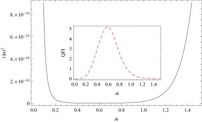
Figure 1: (Color online) The optimal bound $(\Delta\epsilon)^{2}$ in the estimation of the volume ratio $\epsilon$ of the universe over the dimensionless mass $\tilde{m}$ of the Dirac particles. The parameters are fixed with $\epsilon=\tilde{k}=1$. The measurements repeated $n=10^{11}$ times. The QFI (dashed red line) of the Dirac fields as a function of dimensionless mass $\tilde{m}$ for fixed $\epsilon=\tilde{k}=1$.

The adjustable parameters in the probe state Eq.(16) are the dimensionless mass $\tilde{m}$ and the dimensionless momentum $\tilde{k}$ of the particle and antiparticles. Finally, we proceed to compute the error bounds which are our main quantity of interest. The optimal bound for the error in the estimation process can be calculated by using Eqs. (11) and (17). In Fig. (1) we plot the optimal bound $(\Delta\epsilon)^{2}$ in the estimation of the volume ratio $\epsilon$ as a function of dimensionless mass $\tilde{m}$ of the Dirac fields. It is found that the bounds decrease rapidly as the mass for the light Dirac fields increases. We find that there is a finite range of masses that allows for a better estimation of the volume ratio. Thus one can find a method for obtaining the lowest bound by choosing the final projection operator to be on the eigenvectors of the particle states with a chosen mass, determined by the desired outcome. In this way, one can improve the quantum estimation technologies for the volume ratio $\epsilon$ in an expanding universe.

In Fig. (1) we also plot the QFI (dashed red line) of the Dirac fields in the expanding universe as a function of dimensionless mass $\tilde{m}$ for fixed $\epsilon=\tilde{k}=1$. It is interesting to note that in Fig. 2 of Ref. fredericivy1 , the behaviour of entanglement for Dirac fields is very similar with the behaviour of QFI in this paper. Then we arrive to a conclusion that the precision of the estimation of parameters in the expanding universe will be improved from the increase of quantum entanglement. This conclusion corroborate that the precision of quantum parameter estimation can be enhanced if squeezed or entangled states are used as probe systems. For some very larger masses, the QFI diminishes due to the disappearance of quantum entanglement.

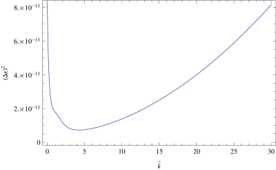
Figure 2: (Color online) The optimal bound $(\Delta\epsilon)^{2}$ in the estimation of the volume ratio $\epsilon$ of the universe over $\tilde{k}$. The parameters are fixed with $\epsilon=\tilde{m}=1$. The measurements repeated $n=10^{11}$ times.

In Fig. (2) we plot the optimal bounds $(\Delta\epsilon)^{2}$ as a function of $\tilde{k}$. The minimum bound is obtained by numerical optimization over $\tilde{k}$. It is shown that the bond $(\Delta\epsilon)^{2}$ deceases at first and then increase as the increasing $\tilde{k}$, which means that the minimum possible bound for the estimation of the volume ratio $\epsilon$ can be find for some optimal $\tilde{k}$. In other words, one can get the highest precision by choosing some fermions with some certain $\tilde{k}$ in the quantum measuring process.

V Conclusions

We studied cosmological quantum metrology by incorporating the effect of universe expansion in quantum parameter estimation. It is shown that the expanding spacetime background changes the value of QFI. At the same time, information about the history of the expanding universe can be extracted from measurements on quantum states in the asymptotic future region. We show that the optimal precision of the estimations depend sensitively on the dimensionless mass $\tilde{m}$ and dimensionless momentum $\tilde{k}$ of the Dirac particles. We find that the precision of the estimation of a parameter in the expanding universe will benefit from the increase of quantum entanglement, which corroborates the fact that the precision can be enhanced if squeezed or entangled states are used as probe systems. It was also shown that the precision of the estimation can be improved by choosing the probe state as an energy eigenvector (i.e., defined by particle number). Such result can be understood from the fact that the largest quantum Fisher information can be obtained by projective measurements corresponding to eigenvectors of the particle states of specific masses and momentums.

- (1) V. Giovanetti, S. Lloyd, and L. Maccone, Nature Photon. 5, 222 (2011).
- (2) S. L. Braunstein and C. M. Caves, Phys. Rev. Lett. 72, 3439 (1994).
- (3) Aasi, J. et al., Nature Photon. 7, 613 (2013).
- (4) P. M. Alsing and G. J. Milburn, Phys. Rev. Lett. 91, 180404 (2003); I. Fuentes-Schuller and R. B. Mann, Phys. Rev. Lett. 95, 120404 (2005).
- (5) T. C. Ralph, G. J. Milburn, and T. Downes, Phys. Rev. A 79, 022121 (2009); J. Doukas and L. C. L. Hollenberg, Phys. Rev. A 79, 052109 (2009); S. Moradi, Phys. Rev. A 79, 064301 (2009).
- (6) M. Aspachs, G. Adesso, and I. Fuentes, Phys. Rev. Lett 105, 151301 (2010).
- (7) S. Khan, M. K. Khan, J. Phys. A: Math. Theor. 44, 045305, (2011); X. Xiao, M. Fang, J. Phys. A 44, 145306 (2011); M. Z. Piao, X. Ji, J. Mod. Optics, 59, 21 (2012); M. Ramzan, Eur. Phys. J. D 67, 170 (2013).
- (8) J. Feng, Y.-Z. Zhang, M. D. Gould, H. Fan, Phys. Lett. B 726, 527(2013); D. J. Hosler and P. Kok, Phys. Rev. A 88, 052112. (2013).
- (9) S. Xu, X.-K. Song, J.-D. Shi, and L. Ye, Phys. Rev. D 89,065022 (2014); J. C. Wang, J. L. Jing and H. Fan, Phys. Rev. D 90, 025032 (2014).
- (10) N. Friis, A. R. Lee, D. E. Bruschi, and J. Louko, Phys. Rev. D 85, 025012 (2012); D. E. Bruschi, I. Fuentes, and J. Louko, Phys. Rev. D 85, 061701(R)(2012).
- (11) N. Friis, A. R. Lee, K. Truong, C. Sabín, E. Solano, G. Johansson, and I. Fuentes, Phys. Rev. Lett. 110, 113602 (2013); E. Martín-Martínez, D. Aasen, and A. Kempf, Phys. Rev. Lett. 110, 160501 (2013).
- (12) Y. Yao, X. Xiao, L. Ge, X. G. Wang, and C. P. Sun, Phys. Rev. A 89, 042336 (2014).
- (13) D. J. Hosler and P. Kok, Phys. Rev. A 88, 052112 (2013).
- (14) M. Aspachs, G. Adesso, and I. Fuentes, Phys. Rev. Lett. 105, 151301 (2010).
- (15) T. G. Downes, G. J. Milburn, and C. M. Caves, arXiv:1108.5220.
- (16) J. Doukas, L. Westwood, D. Faccio, A. Di Falco, and I. Fuentes, Phys. Rev. D 90, 024022 (2014).
- (17) M. Ahmadi, D. E. Bruschi, N. Friis, C. Sabn, G. Adesso, and I. Fuentes, Sci. Rep. 4, 4996 (2014).
- (18) M. Ahmadi, D. E. Bruschi, and I. Fuentes, Phys. Rev. D 89, 065028 (2014).
- (19) C. M. Wilson et al., Nature (London) 479, 376 (2011).
- (20) D. E. Bruschi, N. Friis, I. Fuentes, and S. Weinfurtner, New J. Phys. 15, 113016 (2013); D. E. Bruschi, J. Louko, D. Faccio, and I. Fuentes, New, J. Phys. 15, 073052 (2013).
- (21) X. S. Ma et al., Nature (London) 489, 269 (2012).
- (22) D. E. Bruschi et al., New J. Phys. 16, 053041 (2014).
- (23) D. E. Bruschi, T. Ralph, I. Fuentes, T. Jennewein, and M. Razavi, Phys. Rev. D 90, 045041 (2014).
- (24) J. L. Ball, I. Fuentes-Schuller, and F. P. Schuller, Phys. Lett. A 359, 550 (2006).
- (25) I. Fuentes, R. B. Mann, E. Martín-Martínez, and S. Moradi, Phys. Rev. D 82, 045030 (2010).
- (26) E. Martin-Martinez, and N. C. Menicucci, Class. Quantum Grav. 29, 224003 (2012).
- (27) S. Moradi, R. Pierini, and S. Mancini, Phys. Rev. D 89, 024022 (2014).
- (28) A. Duncan, Phys. Rev. D 17, 964 (1978).
- (29) N.D. Birrell and P.C.W. Davies, Quantum fields in curved space, (CUP 1994).
- (30) L. Bergstrom and A. Goobar, Cosmology and Particle Astrophysics (2nd ed.), (Sprint, 2006).
- (31) M. G. A. Paris, Int. J. Quant. Inf. 7, 125 (2009).
- (32) S. Weinberg, Gravitation and Cosmology: Principles and Applications of the General Theory of Relativity, (Wiley, New York, 1972).
- (33) G. Steigman, Ann. Rev. Nucl. Part. Sci. 29, 313 (1979).
- (34) Alex E. Bernardini, Marcelo M. Guzzo, and Celso C. Nishi, arXiv:1004.0734.
- (35) Benjamin R. Safdi, Mariangela Lisanti, Joshua Spitz, and Joseph A. Formaggio, Phys. Rev. D 90, 043001 (2014).
- (36) D. R. Brill and J. A. Wheeler, Rev. Mod. Phys. 29, 465 (1957); 45, 3888(E) (1992).
- (37) C. Bernard and A. Duncan, Ann. Phys. (N.Y.) 107, 201 (1977).
- (38) Z. X. Wang, D. R Guo. Introduction to Special Function (Peking University Press, Beijing, 2000).
- (39) N. Friis, A. R. Lee, and D. E. Bruschi, Phys. Rev. A 87, 022338 (2013).
- (40) H. Cramr, Mathematical Methods of Statistics (Princeton University, Princeton, NJ, 1946).
- (41) J. Liu, X. X. Jing, and X. G. Wang, Phys. Rev. A 88, 042316 (2013); Y. M. Zhang, X. W. Li, W. Yang, and G. R. Jin, Phys. Rev. A 88, 043832 (2013).