A new class of flexible link functions with application to species co-occurrence in cape floristic region

Abstract

Understanding the mechanisms that allow biological species to co-occur is of great interest to ecologists. Here we investigate the factors that influence co-occurrence of members of the genus Protea in the Cape Floristic Region of southwestern Africa, a global hot spot of biodiversity. Due to the binomial nature of our response, a critical issue is to choose appropriate link functions for the regression model. In this paper we propose a new family of flexible link functions for modeling binomial response data. By introducing a power parameter into the cumulative distribution function (c.d.f.) corresponding to a symmetric link function and its mirror reflection, greater flexibility in skewness can be achieved in both positive and negative directions. Through simulated data sets and analysis of the Protea co-occurrence data, we show that the proposed link function is quite flexible and performs better against link misspecification than standard link functions.

, , ,
and

1 Introduction

Understanding the underlying processes that govern the assembly of biological communities has long been of great interest to ecologists. Obviously, in the absence of species interactions and species habitat preferences, the probability that two species co-occur in a site would simply be the product of the site occupancy probabilities for each of the species. In most biological communities, however, competition [Elton (1946)] and individual response to the environment [Weiher and Keddy (1995)] are likely to play important roles in determining the species composition of local communities. Since phenotypic traits of species and environmental factors could mediate both competition and individual response, the probability of co-occurrence could also be influenced by both the traits of the species and the specific environmental conditions associated with a site. In this study we investigate the processes of community assembly in a well-defined clade, the genus Protea in the Cape Floristic Region (CFR) of southwestern Africa. The response variable, the number of co-occurrences of a certain pair of Protea species, arises naturally as a binomial variable when we define co-occurrence as the number of sites in which two species co-occur within naturally nested watersheds. We take into consideration the spatial association among the co-occurrence of Protea species since it is natural to suspect areas close by would tend to have similar number of co-occurrences as a result of a latent spatial effect. Our primary interest in this study is to build a comprehensive model that could identify important factors influencing the assembly of Protea communities, while adjusting for both spatial association and prevalence of Protea in CFR.

The usual way to model the binomial response is to use a Generalized Linear Model (GLM), where we model the latent probability of “success” by a linear function of covariates through a link function [McCullagh and Nelder (1989)]. The logit, probit and Student $t$ link functions are three of the common links used in GLM. However, the link functions mentioned above are “symmetric” links in the sense that they assume that the latent probability of a given binomial response approaches 0 with the same rate as it approaches 1. Equivalently, the probability density function (p.d.f.) that corresponds to the inverse cumulative distribution function (c.d.f.) of the link function is symmetric. However, this may not be a reasonable assumption in many cases. A commonly adopted asymmetric link function is the complementary loglog (cloglog) link function. However, the cloglog link has a fixed negative skewness. As a result, it lacks both the flexibility to let the data tell how much skewness should be incorporated and the ability to allow for positive skewness. In short, binomial data might often be better modeled with flexible link functions that allow for both positive and negative skew and that allow the data to determine the amount of skewness required.

Much work has been done to introduce flexibility into the link functions. Aranda-Ordaz (1981) proposed two separate one-parameter models for additional flexibility in the logistic model. Guerrero and Johnson (1982) used Box–Cox transformation on the odds ratio to form a more flexible class of model. Jones (2004) proposed a family of flexible distributions based on the distribution of order statistics. Stukel (1988) proposed a two-parameter class of generalized logistic models. Stukel’s model approximates many standard symmetric and asymmetric link functions quite well, but in a Bayesian framework, it may result in improper posteriors when the usual improper uniform prior is used in regressions [Chen, Dey and Shao (1999)]. Kim, Chen and Dey (2008) proposed a class of generalized skewed $t$-link models using a latent variable approach, which achieves proper posteriors for regression coefficients under uniform priors. Unfortunately, the range of the skewness for generalized skewed $t$-link is limited due to a constraint on the shape parameter required for identifiability of the model. More recently, Wang and Dey (2010) propose the generalized extreme value link function to allow more flexible skewness controlled by the shape parameter, but the standard logistic and probit links are not among the special cases of this family.

Several authors have proposed an additional power parameter on the c.d.f. corresponding to standard link functions. Nagler (1994) introduces the Scobit model, which is a generalization of the logistic model by introduction of a power parameter. In the psychology literature, Samejima (2000) proposes the Logistic Positive Exponent Family using similar ideas. These models are part of the asymmetric parametric family proposed by Aranda-Ordaz (1981) under some re-parameterizations. Gupta and Gupta (2008) propose the power normal distribution to accommodate skewness and discuss its advantages over the skew normal distribution. However, even though those link functions with power parameters can accommodate flexible skewness in one direction (e.g., positive skewness in the Scobit link), the skewness in the opposite direction can be asymmetrically limited.

In this paper we propose a new class of symmetric power link functions to model binary and binomial data, and apply it to the Protea species co-occurrence data. The rest of the paper is organized as follows. We introduce the Protea species co-occurrence data in Section 2. In Section 3 we propose a general class of power link functions based on the c.d.f. corresponding to a symmetric baseline link function and its mirror reflection. Section 4 discusses the prior specification and posterior proprieties of the parameter in the proposed model under a fully Bayesian framework. In Section 5 we introduce spatial random effects in the model to account for the spatial association in the co-occurrence data. Section 6 clarifies some computational issues in the model as well as the criteria for model comparisons. Several comprehensive simulation studies are reported in Section 7 with detailed discussions. Finally, in Section 8 we fit the proposed model on the Protea species co-occurrence data. We conclude our paper in Section 9 and all the proofs of the theorems are deferred to the Appendices.

2 The Protea species co-occurrence data

The Cape Floristic Region (CFR) is a region with remarkable biological diversity. The Protea species co-occurrence data we study here is derived from the Protea Atlas data set (http://www.proteaatlas.org.za), which includes 96,253 occurrence records for the 71 species in the genus Protea from 44,415 sites. Wilson and Prunier (unpublished data) constructed a series of nested watersheds covering the CFR using the 3 arc-second (90 m) research-grade digital elevation model collected by the Shuttle Radar Topography Mission (available at http://seamless.usgs.gov) using the r.watersheds function in GRASS [Grass Development Team (2008)]. The co-occurrence data used here correspond to species co-occurrences within watersheds having a mean area of approximately 55 km² ($\pm$40 km²) nested within larger watersheds with a mean area of approximately 540 km² ($\pm$425 km²) [see Figure 1(a) for an illustration of nested watersheds in CFR]. The smaller watersheds are considerably larger than those usually considered in community assembly studies [Vamosi et al. (2009)]. As a result, factors that are associated with a reduced probability of co-occurrence in this analysis may reflect either the consequences of competitive interactions or of habitat segregation among different watersheds.

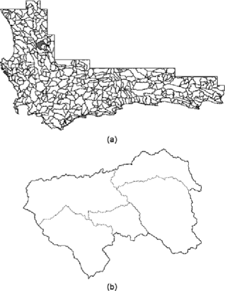
Figure 1: Illustration of the watersheds scale in CFR. (a) The CFR showing the boundaries between the large watersheds within which smaller watersheds are nested. (b) Smaller watersheds nested within one particular parent watershed. This parent watershed is highlighted in grey in part (a).

Figure 2: Histogram of empirical frequencies of Protea species co-occurence.

The data are binomial because for each pair of Protea species, we record the number of smaller watersheds at which a particular pair co-occurs out of the total number of smaller watersheds contained within each larger watershed. The data are then aggregated across the larger watersheds to cover the entire CFR. In this study we record 10,256 observations involving ${71\choose 2}$ pairs of Protea species. In Figure 2 we plot the histogram of observed probability of co-occurrence (number of Protea observed co-occurrences between species pairs divided by the total number of co-occurrences possible). Although this histogram is not excessively skewed, it is reasonable to suspect that an asymmetric link function will be more appropriate for these data, because the histograms for individual species pairs can be very skewed. Our observational unit is species pairs, and for each pair of species we record seven traits that could affect the probability that they co-occur. They are as follows: (1) phylogenetic distance, which is proportional to the time since the two species diverged from a common ancestor, (2) whether or not they differ in fire survival strategy, (3) the difference in plant height, (4) the difference in month of maximum flowering, (5) whether or not they share a pollination syndrome, (6) the difference in leaf area, and (7) the difference in leaf length:width ratio. The difference is measured as either 1:0 for binary data or Euclidean distance for the continuous traits.

Our estimate of phylogenetic distance is derived from a rate-smoothed version of the phylogenetic tree presented in Valente et al. (2010). Specifically, using the topology presented in Valente et al. (2010), we estimated branch lengths under a maximum-likelihood model in PAUP^∗ using the data used to generate the tree: DNA sequences from four chloroplast markers (trnL intron, trnL-trnF spacer, rps16, atpB-rbcL spacer), two nuclear regions (ITS and ncpGS), and 138 AFLP loci. We smoothed the branch lengths using NPRS in r8s [Sanderson (2003)] and calculated pairwise phylogenetic distances using cophenetic.phylo from APE [Paradis, Claude and Strimmer (2004)].

3 The symmetric power link family

Let us first specify the notation used throughout this paper. Suppose $y_{i}\sim\operatorname{Binomial}(p_{i},N_{i})$, where $p_{i}$ is the probability of success for the $i$th observation. Let the design matrix be $\mathbf{X}$ with $x_{i}=(1,x_{i1},x_{i2},\ldots,x_{ik})^{\prime}$ the $i$th row of $\mathbf{X}$ and $\bolds{\beta}=(\beta_{0},\beta_{1},\beta_{2},\ldots,\beta_{k})^{\prime}$ the corresponding regression coefficients. We associate $p_{i}$ and $x_{i}$ through a c.d.f. $F$ as follows:

$$p_{i}=F\bigl{(}x_{i}^{\prime}\bolds{\beta}\bigr{)},$$ (1)

where we call $F^{-1}$ the corresponding link function. The logit, probit, Student $t$ link as well as the cloglog link functions are common links adopted for the binomial regression models.

Here we propose a general class of flexible link functions based on a symmetric baseline link function and its mirror reflection in the following manner. If $F_{0}^{-1}$ is a baseline link function with corresponding c.d.f. $F_{0}$ for which the p.d.f. is symmetric about zero, we propose the symmetric power link family based on $F$ as

$$F(x,r)=F_{0}^{r}\biggl{(}\frac{x}{r}\biggr{)}\mathbf{I}_{(0,1]}(r)+\bigl{[}1-F_{0}^{{1/r}}(-rx)\bigr{]}\mathbf{I}_{(1,+\infty)}(r).$$ (2)

The intuition for the development of (2) is to utilize the fact that $F_{0}^{r}(x)$ is a valid c.d.f. and it achieves flexible left skewness when $r<1$, while the same property holds for its mirror reflection $1-F_{0}^{{1}/{r}}(-x)$ with skewness being in the opposite direction. By combining the two in one single family of link functions, we could achieve flexibility in positive as well as negative skewness symmetrically with respect to the baseline link. Also, we are scaling $x$ by the same parameter $r$ in the formulation to prevent the mode of the p.d.f. to be too far away from zero. Clearly, by introducing an additional parameter $r$ in (2), the skewness of the symmetric power link family can be adjusted from its baseline to achieve more flexibility in modeling asymmetric data.

One immediate observation in (2) is that $F(x,1)=F_{0}(x)$, so the proposed family includes the baseline c.d.f. $F_{0}$ as a special case. Also, considering the fact that $F_{0}$ is symmetric, the proposed symmetric power link family is continuous at the break point $r=1$, since

$$\lim_{r\to 1_{+}}F(x,r)=1-F_{0}(-x)=F_{0}(x)=F(x,1).$$ (3)

As we will be dealing with introduction of flexible skewness into the link function, we specify our measurement of skewness here. We adopt Arnold and Groeneveld’s (1995) skewness measure with respect to the mode here. Under certain conditions, the skewness of a random variable $X$ is defined as $\gamma_{M}=1-2F(M_{x})$, where $F(\cdot)$ is the c.d.f. of $X$ with corresponding mode $M_{x}$. By definition, the skewness is between $-1$ and $1$, with $0$ indicating symmetry. In (2), it follows directly that $F(x,r)=1-F(-x,\frac{1}{r})$. In other words, the p.d.f. of the symmetric power family with power parameter $r$ is the mirror image of the p.d.f. with power parameter $\frac{1}{r}$. This implies that if the skewness of $F(x,r)$ is $\xi$, then the skewness of $F(x,\frac{1}{r})$ will be $-\xi$. Here, by combining the power of a standard symmetric link distribution function and its reflection in one single link, we can accommodate flexible skewness in both directions simultaneously, while retaining the desirable property of having the standard baseline link function as a special case. We propose three symmetric power link function families based on different baseline link functions as follows.

3.1 The symmetric power logit (splogit) link family

If we choose $F_{0}$ to follow the logistic distribution with location 0 and scale 1, then we call $F(x,r)$ defined in (2) the symmetric power logit (splogit) family, and we call the corresponding link function the splogit link. The skewness of the splogit distribution can be found analytically as $\gamma_{M}=1-2(\frac{r}{r+1})^{r}$ for $0<r<1$, and $\gamma_{M}=2(\frac{1}{r+1})^{1/r}-1$ for $r>1$. As a result, it is negatively skewed when $0<r<1$, positively skewed when $r>1$, and reduces to the symmetric logit link when $r=1$. Figure 3(a) and (d) shows the p.d.f. and c.d.f. corresponding

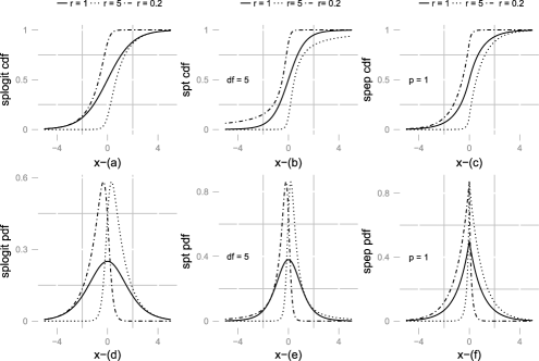
Figure 3: Symmetric power link c.d.f. and p.d.f. for different value of r under logit, Student $t$ and exponential power baseline c.d.f. functions.

to the splogit link with $r=0.2,1,5$, respectively. It is clear that as the power parameter $r$ varies, so does the approaching rate to 0 and 1 for the splogit link. The range of skewness provided by the splogit family is unlimited, reaching $-1$ and 1, respectively, as $r$ tends to 0 and $+\infty$ [see Figure 4(a)].

3.2 The symmetric power $t$ (spt) link family

Many authors have suggested using a Student $t$ link (degrees of freedom denoted as $\nu$) as an alternative to the logit and probit

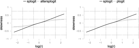
Figure 4: Skewness range of splogit against plogit and altersplogit as $\operatorname{log}(r)$ varies. The possible skewness ranges from $-1$ to 1 under the definition of Arnold and Groeneveld (1995).

links. Mudholkar and George (1978) show that the Student $t$ link with 9 degrees of freedom has the same kurtosis as the logistic distribution. Albert and Chib (1993) suggest using the $t$ distribution with 8 degrees of freedom and provide a full implementation in a Bayesian framework. Liu (2004) proposes the robit model which uses the Student $t$ distribution with known or unknown degrees of freedom as the link function and shows that it is a robust alternative to the logit and probit model. It is widely known that the Student $t$ link with large degrees of freedom approximates the probit link. Now, by bringing in the power parameter $r$ in the sense of (2), we can add more flexible skewness in the class of Student $t$ link functions. We call this new class of link functions the symmetric power $t$ (spt) family. Similarly, in Figure 3(b) and (e) we see the p.d.f. and c.d.f. for the spt link with 5 degrees of freedom for different values of $r$. Clearly, the spt link family allows us to adjust both the skewness of the distribution and the heaviness of the tails by varying $r$ and $\nu$, therefore accounting for an extremely rich class of link functions. In Arnold and Groeneveld’s (1995) sense, the closed form expression of the spt link skewness is not available, but numerically we can show the skewness is quite flexible with small to medium $\nu$ but becomes more restricted as $\nu$ increases. Notice that when $r$ is fixed to be positive, the symmetric power probit distribution is very similar to the power normal distribution proposed by Gupta and Gupta (2008).

3.3 The symmetric power exponential power (spep) link family

The exponential power (ep) distribution was first introduced by Subbotin (1923). The ep distribution is symmetric with density

$$f(x;\mu,\sigma,p)=c^{-1}\operatorname{exp}\biggl{(}-\frac{|z|^{p}}{p}\biggr{)},$$ (4)

where $-\infty<x<+\infty,\sigma>0,p\geq 1,z=(x-\mu)/\sigma$, and $c=2\sigma p^{1/p-1}\Gamma(1/p)$. Clearly, normal distribution is a special case with $p=2$, and heavier tail distribution can be obtained as we set $p$ to be less than 2. Also, the Laplace distribution is another special case when $p=1$. If we set $\mu=0$ and $\sigma=1$, the ep distribution becomes symmetric about zero and with flexible tail properties as $p$ varies. If we set the ep as our baseline link function $F_{0}$, we end up with the symmetric power exponential power (spep) link family [see Figure 3(c) and (f) for the corresponding p.d.f. and c.d.f. for $p=1$ at different values of $r$]. Here we restrict $p$ to be within the range of $[1,2]$ for our proposed spep link family since the skewness of the p.d.f. becomes restricted for $p>2$, that is, with a thinner tail than normal distributions. However, even with this restriction, the spep link family still provides extremely flexible range of skewness and adjustment of tail behavior in one single family of link functions.

3.4 Comparison with other power link

As discussed in Section 1, many authors have proposed to bring in a power parameter to allow more flexible skewness in the link function. Again, let $F_{0}^{-1}$ be the baseline link; the traditional power link family is defined by

$$H(x,r)=F_{0}^{r}(x).$$ (5)

Also, by choosing a different tail in (2), there is an alternative way of constructing the symmetric power link given by choosing the other side of the tail as follows:

$$F^{*}(x,r)=\bigl{[}1-F_{0}^{{1}/{r}}(-rx)\bigr{]}\mathbf{I}_{(0,1]}(r)+F_{0}^{r}\biggl{(}\frac{x}{r}\biggr{)}\mathbf{I}_{(1,+\infty)}(r).$$ (6)

Here, adopting the logit baseline for all three, we compare model (2) (splogit) with model (5) (plogit) and (6) (altersplogit) to illustrate the advantage of our proposed symmetric power link in terms of skewness range. Adopting the other baseline link discussed above will lead to similar results.

The advantage of skewness range of splogit is illustrated in Figure 4. Comparing with plogit, when $\operatorname{log}(r)$ is negative, the skewness of splogit and plogit is exactly the same, which is due to the fact that the formulation of splogit follows closely as plogit when $0<r\leq 1$. However, on the other side, the skewness of splogit reaches 1 as $\operatorname{log}(r)$ goes to infinity, which has a clear advantage over plogit with a skewness limit of 0.264. Similar comparison reveals that by choosing the appropriate side, splogit has skewness advantage on both tails over the altersplogit link. A more flexible skewness means that the probability of success under the splogit link can approach 0 (or 1) in a rate that can never be achieved under the plogit or altersplogit link, which makes it more flexible in dealing with skewed data, as we will show later in the simulation study.

4 The prior and posterior proprieties

We adopt the following class of prior distributions on our proposed symmetric power link family and investigate its posterior proprieties. For regression coefficient $\bolds{\beta}$, we adopt the usual uniform prior, that is, $\pi(\bolds{\beta})\propto 1$. For the power parameter $r$, we adopt a proper gamma prior $\pi(r)$ with mean one and reasonably large variance. If we denote the likelihood of the model to be $\mathbf{L}(\bolds{\beta},r|\mathbf{y})$, consequently, the joint posterior density of our regression model becomes

$$\pi(\bolds{\beta},r|\mathbf{y}) \propto \mathbf{L}(\bolds{\beta},r|\mathbf{y})\pi(\bolds{\beta})\pi(r)$$

$$\propto \prod_{i=1}^{n}\bigl{[}F\bigl{(}x_{i}^{\prime}\bolds{\beta},r\bigr{)}\bigr{]}^{y_{i}}\bigl{[}1-F\bigl{(}x_{i}^{\prime}\bolds{\beta},r\bigr{)}\bigr{]}^{1-y_{i}}\pi(r).$$

Clearly, the posterior distribution is proper if and only if

$$\int_{\Re^{+}}\int_{\Re^{k}}\mathbf{L}(\bolds{\beta},r|\mathbf{y})\pi(r)\,d\bolds{\beta}\,dr<\infty.$$ (8)

Notice that when $r$ is a point mass at 1, $F(x,r)$ becomes the baseline link function $F_{0}$. Our goal is to investigate whether the introduction of a power parameter $r$ would change the posterior propriety compared to merely adopting the symmetric baseline function $F_{0}$. Here we let $\mathbf{L}_{0}(\bolds{\beta}|y)$ denote the likelihood under the corresponding baseline link $F_{0}$.

Theorem 1.

If under the baseline link $F_{0}$ we have

$$\int_{\Re^{k}}\mathbf{L}_{0}(\bolds{\beta}|\mathbf{y})\,d\bolds{\beta}<\infty,$$ (9)

then the posterior under the corresponding power link $\pi(\bolds{\beta},r|\mathbf{y})$ is also proper, that is,

$$\int_{\Re^{+}}\int_{\Re^{k}}\mathbf{L}(\bolds{\beta},r|\mathbf{y})\pi(r)\,d\bolds{\beta}\,dr<\infty.$$ (10)

Theorem 1 states that by introducing an additional power parameter $r$ in the sense of (2), the posterior propriety under the uniform $\bolds{\beta}$ prior is unchanged with a proper prior for $r$. Chen and Shao (2001) studied the conditions for the propriety of the posterior distribution under general link functions. The following theorem resolves the posterior proprieties of the three proposed symmetric power link families under uniform $\bolds{\beta}$ priors. For the spt and spep link families, throughout this paper we adopt proper priors on $\nu$ and $p$.

Theorem 2.

Let $\tau_{i}=1$ if $y_{i}=0$ and $\tau_{i}=-1$ if $y_{i}=1$, and define $\mathbf{X}^{*}$ to be the matrix with the $i$th row $\tau_{i}x_{i}^{\prime}$. Suppose the following conditions hold:

The design matrix $\mathbf{X}$ is of full column rank.

There is a positive vector $\mathbf{a}=(a_{1},a_{2},\ldots,a_{n})^{\prime}\in\Re^{n}$ such that $\mathbf{a}^{\prime}\mathbf{X}^{*}=0$.

Then the proposed splogit and spep links lead to proper posteriors under the above prior setup, while the same result also holds for the spt family with degrees of freedom $\nu>k$, where $k$ is the number of columns of $\mathbf{X}$.

5 Spatial random effects

Geological and climatic features vary greatly across the CFR. For example, the climate in the western part of CFR is Mediterranean with rainfall concentrated in the winter months, while the climate in the eastern CFR is more aseasonal. While such climate features could affect the pattern of Protea co-occurrence, we are primarily interested in identifying biological features that influence co-occurrence. Thus, we add spatial random effects in the model to account for all latent, unmeasured environmental effects that are spatially structured. Here we use the intrinsically conditionally autoregressive (ICAR) model [Besag and Green (1993)] to capture these spatial effects. The ICAR model has gained increasing usage in the past two decades due to its convenient implementation in the context of Gibbs sampling for fitting hierarchical spatial models [Banerjee, Carlin and Gelfand (2004)].

In the Protea co-occurrence context we suppose that there are $K$ parent watersheds and that the proximity matrix $A$ is defined by $A_{ij}=1$ if watersheds $i$ and $j$ are adjacent and $A_{ij}=0$ otherwise. Following notation in Section 3, the number of co-occurrence between species $l$ and $m$ within watershed $k$ is modeled as

$$y_{lmk} \sim \operatorname{Binomial}(p_{lmk},N_{k}),$$ (11)

$$p_{lm} = F\bigl{(}x_{lm}^{\prime}\bolds{\beta}+w_{k}\bigr{)},$$ (12)

where $N_{k}$ is the number of smaller watersheds within parent watershed $k$, and $w_{k}$ is the spatial random effect associated with watershed $k$, where $k=1,2,\ldots,K$. At the next stage, the spatial random effects $(w_{1},w_{2},\ldots,w_{K})$ follow the ICAR model, that is,

$$p(w_{1},w_{2},\ldots,w_{K})\propto\operatorname{exp}\biggl{[}-\frac{1}{2\tau^{2}}\sum_{i\neq j}A_{ij}(w_{i}-w_{j})^{2}\biggr{]}.$$ (13)

Clearly, (13) is not a proper distribution, so it cannot be used to model data directly. However, here we use it as a prior distribution on the second stage of the hierarchical model which avoids this problem. In addition, to make $\mathbf{w}$ fully identifiable, we impose the constraint $\sum_{k}w_{k}=0$.

6 Computational issues

6.1 Markov chain Monte Carlo (MCMC) sampling

The posterior distribution given in (4) is relatively easy to sample given the standard baseline link c.d.f. $F_{0}$. To run the Gibbs sampler, we subsequently sample from the complete conditional distributions $[\bolds{\beta}|r,\mathbf{y}]$, $[r|\bolds{\beta},\mathbf{y}]$ (also $[\nu|\bolds{\beta},r,\mathbf{y}]$ if under spt and $[p|\bolds{\beta},r,\mathbf{y}]$ if under spep). Each draw can be done using the Adaptive Rejection Metropolis algorithm [Gilks, Best and Tan (1995)] which is implemented in JAGS [Plummer (2003)]. Due to the conditional nature of the ICAR distribution, the Gibbs sampler of spatial random effects is conveniently constructed and the details are discussed in Banerjee, Carlin and Gelfand (2004). All the computations in this paper are done in JAGS or geoBUGS.

6.2 Covariate effects

Czado and Santner (1992) pointed out that it is more appropriate to compare the covariate effects under different link functions with the estimated probabilities since the estimates of $\bolds{\beta}$ will depend on the choice of link functions. In view of this, we use the method suggested by Chib and Jeliazkov (2006) to calculate the average effect of the covariates estimated probabilities. Here we denote the set of all parameters in our model to be $\bolds{\theta}$. For example, if we want to estimate the effect of covariate $x_{i}$, we integrate out parameters $\bolds{\theta}$ by its MCMC posterior samples, and marginalize out other covariates $\mathbf{x}_{-i}$ by their empirical distributions to get an estimate of the predictive distribution

$$[p|x_{i},\mathbf{y}]=\int[p|x_{i},\mathbf{x}_{-i},\bolds{\theta},\mathbf{y}]\pi(\bolds{\theta}|\mathbf{y})\pi(\mathbf{x}_{-i})\,d\bolds{\theta}\,d\mathbf{x}_{-i}.$$ (14)

Then if we compute this estimated probability under two specific values of $x_{i}$, for example, under 0 and 1, the difference in the computed probabilities gives an estimated effect of covariates $x_{i}$ as it changes from 0 to 1.

6.3 Bayesian model comparison

To compare the performance of models under different link functions, we calculate two summary measures. The first one is the Deviance Information Criterion (DIC), which balances the fit of a model to the data with its complexity. The DIC measure is calculated with the posterior mean of deviance penalized by the effective number of parameters under the Bayesian framework [Spiegelhalter et al. (2002)]. The other measure we consider here is the logarithm of the pseudo-marginal likelihood (LPML), which measures the accuracy of prediction based on leave-one-out cross-validation ideas. The LPML measure [Ibrahim, Chen and Sinha (2005)] is a summary statistic of the conditional predictive ordinate (CPO) criterion [Gelfand, Dey and Chang (1992)]. The model with the larger LPML indicates better fit of competing models.

7 Simulation study

Here we conduct three sets of simulation studies. The first one compares the performance of our proposed symmetric power link function against some other standard or flexible link functions. The second one focuses on the performance of splogit link versus plogit link when the data is generated by a skewed distribution. The third one investigates specifically how our proposed model performs against other flexible link functions on a larger scale simulation. To simplify our simulation, here we consider Bernoulli responses instead of binomial. Before we go any further, we introduce two other flexible link functions for comparison purposes.

Stukel (1988) proposed the generalized logistic link family with parameter $\bolds{\alpha}=(\alpha_{1},\alpha_{2})^{\prime}$ as follows:

$$p_{i}=G\bigl{(}h_{\alpha}\bigl{(}x_{i}^{\prime}\bolds{\beta}\bigr{)}\bigr{)},$$

where $G$ is the c.d.f. of the logistic distribution. When $x_{i}^{\prime}\bolds{\beta}\geq 0$,

$$h_{\alpha}\bigl{(}x_{i}^{\prime}\bolds{\beta}\bigr{)}=\cases{\alpha_{1}^{-1}\bigl{(}\operatorname{exp}\bigl{(}\alpha_{1}x_{i}^{\prime}\bolds{\beta}\bigr{)}-1\bigr{)},&\quad$\alpha_{1}>0$,\vspace*{1pt}\cr x_{i}^{\prime}\bolds{\beta},&\quad$\alpha_{1}=0$,\cr-\alpha_{1}^{-1}\operatorname{log}\bigl{(}1-\alpha_{1}x_{i}^{\prime}\bolds{\beta}\bigr{)},&\quad$\alpha_{1}<0$,}$$

and for $x_{i}^{\prime}\bolds{\beta}\leq 0$,

$$h_{\alpha}\bigl{(}x_{i}^{\prime}\bolds{\beta}\bigr{)}=\cases{-\alpha_{2}^{-1}\bigl{(}\operatorname{exp}\bigl{(}\alpha_{2}\bigl{|}x_{i}^{\prime}\bolds{\beta}\bigr{|}\bigr{)}-1\bigr{)},&\quad$\alpha_{2}>0$,\vspace*{1pt}\cr x_{i}^{\prime}\bolds{\beta},&\quad$\alpha_{2}=0$,\cr\alpha_{2}^{-1}\operatorname{log}\bigl{(}1-\alpha_{2}\bigl{|}x_{i}^{\prime}\bolds{\beta}\bigr{|}\bigr{)},&\quad$\alpha_{2}<0$.}$$

Also, Czado (1994) proposed another two parameters family link functions given by specifying

$$h_{\alpha}\bigl{(}x_{i}^{\prime}\bolds{\beta}\bigr{)}=\cases{\displaystyle\frac{(x_{i}^{\prime}\bolds{\beta}+1)^{\alpha_{1}}-1}{\alpha_{1}},&\quad$x_{i}^{\prime}\bolds{\beta}\geq 0$,\vspace*{2pt}\cr\displaystyle-\frac{(-x_{i}^{\prime}\bolds{\beta}+1)^{\alpha_{2}}-1}{\alpha_{2}},&\quad$x_{i}^{\prime}\bolds{\beta}<0$.}$$

First we compare splogit link with other link functions with detailed simulation. We generate 2 covariates for our simulation study. We independently generate one binary covariate $x_{1}$ with 0 and 1 randomly chosen, and the second covariate $x_{2}$ is generated independently from $N(0,3)$. Our vector of covariates is denoted as $X=(1,x_{1},x_{2})^{\prime}$. The true regression coefficient $\bolds{\beta}=(\beta_{0},\beta_{1},\beta_{2})^{\prime}$ is set to be $(0,1,1)^{\prime}$ for all simulations. With the same value of $X^{\prime}\beta$, we carry out our studies under three scenarios based on three true models as follows:

Scenario 1.

The binary data are generated from the symmetric logistic link model with $F^{-1}(p_{i})=\operatorname{log}(p_{i}/(1-p_{i}))$.

Scenario 2.

The binary data are generated from the complementary loglog (cloglog) link with $F^{-1}(p_{i})=\operatorname{log}(-\operatorname{log}(1-p_{i}))$. It is easily calculated that the skewness of the corresponding $F$ is $-0.264$, under the definition of Arnold and Groeneveld (1995).

Scenario 3.

The binary data are generated from the loglog link with $F^{-1}(p_{i})=-\operatorname{log}(-\operatorname{log}(p_{i}))$. The corresponding $F$ is the mirror reflection of the c.d.f. corresponding to the cloglog link, and therefore with skewness $0.264$.

As described in Section 6, we conduct a fully Bayesian analysis on the above three simulated data sets. The prior of $\beta$ is chosen to be $N(0,10^{4})$ and the prior for $r$ is set to be exponential with parameter 1. In the spt model the prior for $\nu$ is chosen to be $\operatorname{Gamma}(8,1)$ and for the spep model the prior for $p$ is chosen to be $\operatorname{unif}(1,2)$. In the “Stukel” and “Czado” models, the priors for parameters $a_{1}$ and $a_{2}$ are set to be $N(0,10^{2})$. For each scenario, we repeat the same setting for two different sample sizes $N=500$ and $N=2000$ to see how sample size would affect our inference. After 2000 burn-ins, the models mix pretty well and we obtain 4000 posterior samples for each parameter. We summarize DIC and LPML measures in order to make model comparisons. Our simulation results are summarized in Table 1 and in Figure 5.

= True model Fitted model logit cloglog loglog $\bolds{\beta_{1}}$ $\bolds{\beta_{2}}$ $\bolds{\nu/p}$ LPML DIC $\bolds{\beta_{1}}$ $\bolds{\beta_{2}}$ $\bolds{\nu/p}$ LPML DIC $\bolds{\beta_{1}}$ $\bolds{\beta_{2}}$ $\bolds{\nu/p}$ LPML DIC $\mbox{Sample size}=500$ logit 0.12 0.11 $\bolds{-}$180.6 0361.1 0.15 0.06 $-$137.6 $274.7$ 0.13 0.17 $-$136.9 $273.6$ cloglog 0.10 0.15 $-$184.3 $367.4$ 0.15 0.05 $\bolds{-}$131.1 0262.1 0.12 0.23 $-$145.1 $289.5$ loglog 0.15 0.09 $-$189.2 $375.4$ 0.14 0.06 $-$161.2 $317.4$ 0.14 0.14 $\bolds{-}$134.4 0268.6 Stukel 0.11 0.09 $-$183.4 $365.8$ 0.16 0.04 $-$131.7 $261.5$ 0.13 0.14 $-$137.2 $270.5$ Czado 0.11 0.10 $-$182.4 $363.9$ 0.16 0.04 $-$132.0 $262.3$ 0.13 0.14 $-$136.7 $269.7$ splogit 0.12 0.11 $-$181.0 $359.7$ 0.15 0.05 $-$131.5 $262.1$ 0.13 0.16 $-$135.9 $270.9$ spt 0.12 0.11 7.23 $-$181.1 $360.5$ 0.15 0.04 6.02 $-$131.7 $261.9$ 0.13 0.16 7.43 $-$136.4 $271.7$ spep 0.11 0.11 1.41 $-$181.2 $360.6$ 0.15 0.05 1.23 $-$132.6 $264.0$ 0.13 0.16 1.38 $-$135.9 $270.9$ $\mbox{Sample size}=2000$ logit 0.13 0.10 $\bolds{-}$696.6 1393.1 0.09 0.04 $-$491.3 $982.5$ 0.11 0.16 $-$507.0 $1013.9$ cloglog 0.13 0.14 $-$711.6 $1422.0$ 0.09 0.02 $\bolds{-}$477.7 0955.6 0.11 0.22 $-$544.7 $1088.0$ loglog 0.12 0.08 $-$730.3 $1457.4$ 0.09 0.05 $-$525.8 $1050.0$ 0.11 0.13 $\bolds{-}$500.6 1000.9 Stukel 0.13 0.10 $-$698.5 $1396.7$ 0.10 0.02 $-$478.9 $956.6$ 0.10 0.14 $-$501.8 $1003.5$ Czado 0.13 0.10 $-$698.3 $1396.2$ 0.10 0.02 $-$479.0 $957.1$ 0.10 0.13 $-$501.4 $1002.8$ splogit 0.13 0.10 $-$696.9 $1392.9$ 0.09 0.02 $-$481.2 $962.4$ 0.11 0.13 $-$501.4 $1002.2$ spt 0.13 0.10 7.21 $-$697.5 $1394.2$ 0.09 0.03 9.50 $-$483.1 $966.4$ 0.11 0.13 8.54 $-$502.3 $1004.1$ spep 0.12 0.10 1.40 $-$697.5 $1394.1$ 0.09 0.03 1.43 $-$478.9 $956.9$ 0.10 0.15 1.34 $-$501.7 $1002.4$

Table 1: Posterior covariate effects for $\beta_{1}$ and $\beta_{2}$, posterior median for $\nu$ and $p$ in spt and spep models as well as model comparisons under sample sizes 500 and 2000. Bold numbers indicate the corresponding fit is under the true model. Covariate effects are measured between value 0 and 1. Larger LPML and smaller DIC indicate a better fit

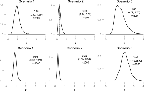
Figure 5: Posterior density plot for power parameter $r$ under the splogit model with sample sizes 500 and 2000. The posterior median and HPD interval of $r$ are also reported in the plot.

We notice from Figure 5 that under sample sizes of both 500 and 2000, the posterior mean of $r$ in the splogit link is close to 1 when the true model is logit (symmetric), significantly less than 1 when the true model is cloglog (left-skewed), and significantly greater than 1 when the true model is loglog (right skewed). Not surprisingly, the posterior standard deviation of $r$ becomes considerably smaller as the sample size increases from 500 to 2000. Also, the performance of $r$ in the spt and spep links is quite similar to the splogit link shown in Figure 5. In conclusion, the power parameter $r$ captures the skewness of the true model very well.

Table 1 summarizes some other simulation results of the study. Comparing with standard links (logit, cloglog, loglog), calculated average covariate effect of $\beta_{1}$ and $\beta_{2}$ for the symmetric power links tends to be much closer to the value under the true model (bold) than other standard models (logit, cloglog, loglog when it is not the true model). We also observed that the symmetric power link provides estimates of covariate effects that are extremely close to the true model and significantly better than other standard link functions in terms of LPML and DIC. On the other hand, the symmetric power link performs extremely close to “Stukel” and “Czado” models in terms of both covariate effects and model comparisons. Overall, our proposed model performs well and proves to be robust enough to handle various scenarios under simulated data with symmetric, positive and negative skewness.

We conduct the second simulation study to examine the performance of the splogit link against the plogit link (5) and altersplogit link (6), when the data is generated from distributions with various skewness. We simulate data from the generalized extreme value (gev) distribution with c.d.f. as follows:

$$G(x)=\operatorname{exp}\biggl{[}-\biggl{(}1+\xi\frac{x-\mu}{\sigma}\biggr{)}_{+}^{-{1}/{\xi}}\biggr{]}.$$ (15)

Wang and Dey (2010) propose the gev model as another flexible link function to model binary response data. The skewness of (15) is controlled by the shape parameter $\xi$, which is calculated as $1-2\operatorname{exp}\{-(1+\xi)\}$ under Arnold and Groeneveld’s (1995) definition. Notice that $\xi=-0.3$ indicates the skewness is zero. To simulate data from the gev distribution, we set $F$ to be $G$ with $\mu=0$, $\sigma=1$, and adopt the same covariates setup as in the first study. We choose $\xi=-3.3,-0.3,2.7$, respectively, to represent left-skewed, symmetric and right-skewed data. For each value of $\xi$, we generate 100 data sets and fit splogit against plogit and altersplogit, respectively, to compare the average performance of the two. Again, we obtain 4000 posterior samples for each simulation after 2000 burn-in periods.

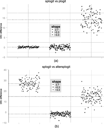
Figure 6: Difference of DIC comparing (a) splogit and plogit, (b) splogit and altersplogit when shape parameter $\xi=-3.3,-0.3,2.7$, respectively. Positive DIC difference indicates splogit has a better fit. In each case the simulation is repeated 100 times. The dotted line indicates the mean of DIC for the repetitions.

Figure 6 summarizes the difference of DIC between the model fits under splogit and plogit (a), splogit and altersplogit (b) of 100 replicates for each simulation. For (a), the advantage of using the average DIC of splogit is not obvious when $\xi=-3.3,-0.3$, but becomes positive at $\xi=2.7$. For (b), the average DIC advantage of splogit is positive at $\xi=-3.3,2.7$, but ignorable at $\xi=-0.3$. This is exactly what we expected by looking at Figure 4 in that the splogit has skewness advantage over plogit when the data is left skewed, and has skewness advantage over altersplogit in both skewness directions.

In the third study we compare the performance of the splogit model against gev, “Stukel” and “Czado” models on a larger scale, while only focusing on model comparisons. Here, by larger scale we mean repeating the fitting of all 4 models 200 times under different true models, and record the best performance each time according to the DIC measure. To simplify the comparison, we pick sample size $N=200$ and generate one continuous covariate from standard normal distribution. For each of the 200 simulations, the true value of $\bolds{\beta}=(\beta_{0},\beta_{1})^{\prime}$ is generated from $N(1,0.1^{2})$. The prior setups of splogit, “Stukel” and “Czado” are the same as before, while the prior of $\xi$ in the gev model is set to be $\operatorname{uniform}(-1,1)$. The simulation scheme is also similar to the first study, as we set the true model to be from logit, cloglog and loglog, then we fit splogit, gev, “Stukel” and “Czado” models, respectively, to find the percentage of best performance in terms of DIC.

=288pt % Lowest DIC True model splogit gev Stukel Czado logit 49.5% 31.0% 19.5% 0%0. cloglog 26.5% 62.5% 08.5% 2.5% loglog 63.0% 09.0% 24.0% 4.0%

Table 2: Percentage of best performance among splogit, gev, “Stukel” and “Czado” out of 200 simulations. The best performance is determined each time by the lowest DIC value

In Table 2 we clearly see the advantage of the proposed splogit link over other link functions. The splogit link model performs the best when the true model is logit and loglog at 49.5% and 63.0%, respectively, where the gev model and “Stukel” model come as distant second places with 31.0% and 24.0%. The gev model outperforms splogit when the true model is cloglog, however, this is expected since cloglog is a special case of a gev model when $\xi=0$. Nevertheless, in the cloglog case, the splogit model performs better than “Stukel” and “Czado” models at 26.5%. Overall, we see the robustness of the proposed splogit link against other flexible link functions.

8 Data analysis

Here we apply the model described in Section 3 on the Protea species co-occurrence data. The data is provided as supplementary material [Jiang et al. (2013)]. As discussed earlier, we include phylogenetic distance (GD), fire survival strategy (FSS), plant height, month of maximum flowering (MMF), pollination syndrome, specific leaf area (SLA) and leaf length width ratio (LWR) as factors in the model and prevalence probability (with a logit transformation) as a covariate. Among them, FSS, MMF and pollination are binary and the rest are continuous. Notice that in order to model the species co-occurrence, Palmgren (1989) proposed a method of running two logistic regressions on two species separately and related the two with a regression on odds ratio. While it is no problem to

= splogit plogit logit gev Variables Median HPD interval Median HPD interval Median HPD interval Median HPD interval Modeling $P(y=1)$ Intercept $-$0.294 ($-$0.354, $-$0.235) $-$0.300 ($-$0.349, $-$0.248) 0.457 (0.407, 0.509) 0.019 ($-$0.023, 0.063) GD 0.019 (0.005, 0.033) 0.019 (0.004, 0.032) 0.032 (0.013, 0.052) 0.020 (0.002, 0.036) FSS 0.025 ($-$0.004, 0.059) 0.025 ($-$0.002, 0.050) 0.053 (0.010, 0.098) 0.027 ($-$0.007, 0.059) Height $\bolds{-}$0.023 ($-$0.038, $-$0.009) $\bolds{-}$0.023 ($-$0.038, $-$0.009) $\bolds{-}$0.032 ($-$0.052, $-$0.012) $\bolds{-}$0.026 ($-$0.043, $-$0.008) MMF 0.013 ($-$0.026, 0.052) 0.014 ($-$0.026, 0.050) 0.037 ($-$0.014, 0.092) 0.014 ($-$0.031, 0.058) Pollination $-$0.029 ($-$0.060, 0.004) $-$0.029 ($-$0.057, 0.001) $-$0.030 ($-$0.073, 0.011) $\bolds{-}$0.038 ($-$0.074, $-$0.003) SLA $-$0.003 ($-$0.017, 0.011) $-$0.003 ($-$0.018, 0.010) $-$0.006 ($-$0.024, 0.012) $-$0.006 ($-$0.022, 0.010) LWR $\bolds{-}$0.027 ($-$0.044, $-$0.012) $\bolds{-}$0.027 ($-$0.043, $-$0.011) $\bolds{-}$0.037 ($-$0.059, $-$0.017) $\bolds{-}$0.031 ($-$0.051, $-$0.013) Prevalence 0.844 (0.815, 0.873) 0.842 (0.818, 0.866) 1.146 (1.125, 1.164) 0.991 (0.963, 1.016) $r/\xi$ 0.380 (0.331, 0.0431) 0.376 (0.336, 0.423) 0.042 (0.020, 0.062) DIC 23,002.0 23,001.0 23,335.2 23,006.3 Modeling $P(y=0)$ Intercept 0.295 (0.249, 0.333) 0.313 (0.293, 0.327) $-$0.456 ($-$0.508, $-$0.406) $-$0.579 ($-$0.609, $-$0.547) GD $\bolds{-}$0.019 ($-$0.033, $-$0.003) $\bolds{-}$0.008 ($-$0.014, $-$0.003) $\bolds{-}$0.032 ($-$0.051, $-$0.012) $\bolds{-}$0.015 ($-$0.026, $-$0.003) FSS $-$0.024 ($-$0.051, 0.005) $\bolds{-}$0.013 ($-$0.026, $-$0.002) $\bolds{-}$0.054 ($-$0.097, $-$0.011) $\bolds{-}$0.026 ($-$0.047, $-$0.003) Height 0.023 (0.009, 0.037) 0.009 (0.003, 0.015) 0.031 (0.010, 0.051) 0.017 (0.005, 0.029) MMF $-$0.013 ($-$0.053, 0.023) $-$0.008 ($-$0.024, 0.008) $-$0.037 ($-$0.091, 0.016) 0.006 ($-$0.024, 0.038) Pollination 0.030 ($-$0.001, 0.059) 0.009 ($-$0.004, 0.021) 0.029 ($-$0.014, 0.072) 0.022 ($-$0.002, 0.045) SLA 0.003 ($-$0.010, 0.018) 0.002 ($-$0.004, 0.008) 0.006 ($-$0.013, 0.024) 0.006 ($-$0.005, 0.017) LWR 0.028 (0.012, 0.045) 0.011 (0.004, 0.017) 0.037 (0.015, 0.058) 0.022 (0.009, 0.035) Prevalence $\bolds{-}$0.845 ($-$0.866, $-$0.818) $\bolds{-}$0.340 ($-$0.380, $-$0.294) $\bolds{-}$1.146 ($-$1.166, $-$1.127) $\bolds{-}$0.677 ($-$0.686, $-$0.669) $r/\xi$ 2.624 (2.344, 2.948) 2.998 (2.693, 3.441) $\bolds{-}$0.639 ($-$0.661, $-$0.619) DIC 23,001.8 23,069.1 23,335.0 23,101.5

Table 3: Posterior median, HPD interval and DIC measure under splogit, plogit, gev, logit models of the Protea co-occurrence data. The first half of the table models $P(y=1)$, while the second half models $P(y=0)$. Bold numbers indicate significant factors. Smaller DIC indicates better fit

integrate our sp link in the Palmgren model to replace the logit link, it is not suitable for our particular data since the co-occurrence data has the traits difference between two species, but not the traits of two species separately. For simplicity, we only adopt splogit as a representative of the symmetric power link family, however, adopting the spt and spep links would lead to similar results. After 10,000 burn-ins the model parameters and spatial random effects mix pretty well and then another 10,000 samples have been obtained. Table 3 summarizes the results under different links with ICAR prior on the spatial random effects. The priors of the regression coefficients are set to be normal with mean $0$ and variance $10^{4}$. The spatial model is realized utilizing GeoBUGS, an add-on to WinBUGS [Lunn et al. (2000)].

First, let us look at the first half of Table 3. When we model the probability of co-occurrence, that is, $P(y=1)$, we see that for the splogit and plogit models the estimate of the power parameter is around 0.38, corresponding to a left-skewed link. Recall that splogit is equivalent to plogit when $r\leq 1$. As a result, parameter estimates and model comparison criteria for the splogit and plogit are roughly the same. The gev model with an estimate of $\xi=0.042$ also corresponds to a left-skewed model with a DIC slightly worse than splogit and plogit. Finally, all three flexible links perform much better than logit in terms of DIC.

In order to show the advantage of the splogit link, the second half of Table 3 considers the probability of not co-occurring, $P(y=0)$, instead. We notice that due to the symmetric construction of splogit, modeling $P(y=0)$ and $P(y=1)$ are essentially the same, the only change being in the sign of the parameters. Here we can see that the parameter estimates and model comparison criterion value of splogit and plogit are different and splogit has a clear edge in terms of model comparison. These results are consistent with analytical expectations and our simulations: splogit and plogit are equivalent when $r\leq 1$, but when $r>1$, splogit performs better than plogit. In the gev model, the estimate of $\xi=-0.639$ now corresponds to a right-skewed model, and with a DIC of 23,101.5, the gev model fits worse than splogit and plogit. Again, all three of them fit better than the standard logit link. Figure 7 plots probability curves under splogit, plogit, logit and gev links as different covariates vary in modeling $P(y=0)$. We see that the curve under splogit has a more flexible tail behavior that results in a better fit.

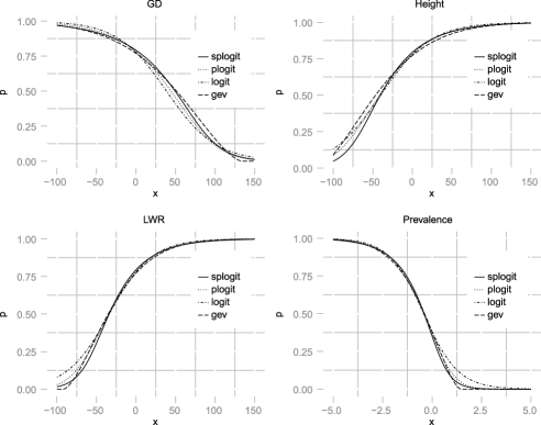
Figure 7: Probability curves under splogit, plogit, logit and gev links as different covariates vary in modeling $P(y=0)$. GD, Height, LWR and Prevalence are chosen since they are significant in all three models. Other covariates are fixed to be at the mean and coefficients are fixed to be at the posterior median.

In one sense, it is not surprising that “Prevalence” is the predominant influence on the probability of co-occurrence. Let $n_{ik}$ be the number of small watersheds in which species $i$ is found in watershed $k$ and $n_{k}$ be the number of small watersheds in watershed $k$. Then $p_{ik}=(n_{ik}+1)/(n_{k}+2)$ is the probability that species $i$ is found in watershed $k$, and the prevalence of the species pair $i$ and $j$ in watershed $k$ is $p_{ik}p_{jk}$. In short, if two species are both common within a watershed, they are likely to co-occur, and if they are both uncommon, they are unlikely to co-occur.

In another sense, however, the importance of “Prevalence” may be surprising. It indicates that to a large extent species co-occur or not as if they were randomly assigned to small watersheds, suggesting that the biotic factors included in our analysis have relatively little effect on whether or not they co-occur. Competitive effects, if they existed, would lead similar species to co-occur less often than expected [corresponding to negative regression coefficients when modeling $P(y=1)$]. It may not be surprising that competitive effects are small in this analysis, since the small watershed scale is much larger than the scale at which individual plants would compete, but habitat partitioning among watersheds would lead to the same pattern. Thus, the small negative coefficients associated with “Height” and “LWR” (leaf length-width ratio) suggest not only that competitive effects on the structure of Protea communities at this scale, if any, are small, but also that habitat partitioning has a similarly small influence on the probability of co-occurrence.

We regard “GD” (phylogenetic distance) as a proxy for unmeasured traits that influence co-occurrence, and the positive coefficient on it may be surprising. Its magnitude is similar to that of the negative coefficients on “Height” and “LWR,” and it is small relative to “Prevalence,” but the positive sign indicates that closely related taxa occurring in the same large watershed are more likely to co-occur within small watersheds than expected by chance. Perhaps this association reflects some degree of habitat filtering [Shipley, Vile and Garnier (2006), Weiher and Keddy (1995)] on traits that we did not measure in this study.

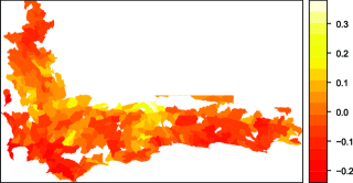
Figure 8: Plot of spatial random effects in CFR under splogit fit.

The spatial clustering effects on co-occurrence probabilities are also obvious. In Figure 8 we see negative effects clustered in the east part and southwest corner of CFR, while positive effects are clustered in the middle part of the region. This clustering could reflect the interaction of rainfall (winter rainfall in the west, aseasonal in the east) and elevation (highest elevations inland, lowest along the coast). In future studies, we will explore both the patterns of co-occurrence at different spatial scales and the extent to which climate or other environmental features are associated with residual spatial variation in this analysis.

9 Discussion

In this paper we introduced a new family of flexible link functions. The proposed power link family can accommodate flexible skewness in both positive as well as negative directions, while retaining the baseline standard link as a special case. Simulation results show the proposed link performs well under various skewness scenarios. Also, the proposed link is computationally straightforward and efficient to implement. In addition, the power parameter idea illustrated here may be used to construct new link functions. For example, we could use an asymmetric link function c.d.f. as our baseline link. Using a power parameter might make a difference in bringing in desirable flexibility.

One potential problem with the proposed power link is that the power parameter $r$ influences both the skewness and the mode of the link function p.d.f. Although this effect has been greatly reduced by scaling $x$ by $r$ in our model as defined in (2) and discussed in Section 3, the effect still exists with relatively large $r$ values. One solution might be to adjust the effect out with calculated mode values, yet it is computationally expensive especially under pt and pep links when there is no analytical solution for the mode of the c.d.f. function.

Appendix A Proof of Theorem 1

Observing that in our definition the power link functions $F_{r}$ naturally split with respect to $r=1$, we have

$$\int_{\Re^{+}}\int_{\Re^{k}}\mathbf{L}(\bolds{\beta},r|\mathbf{y})\pi(r)\,d\bolds{\beta}\,dr$$

$$\qquad=\int_{0}^{1}\int_{\Re^{k}}\mathbf{L}(\bolds{\beta},r|\mathbf{y})\pi(r)\,d\bolds{\beta}\,dr+\int_{1}^{\infty}\int_{\Re^{k}}\mathbf{L}(\bolds{\beta},r|\mathbf{y})\pi(r)\,d\bolds{\beta}\,dr.$$

Clearly, the link function in the latter part is the mirror reflection of the first part, in other words, $F(x,r)=1-F(-x,\frac{1}{r})$, therefore, we only need to prove the first part of the integration is finite. For the baseline link $F_{0}$ we have

$$F_{0}(x) = \int_{\Re}I(u\geq-x)\,d\bigl{(}-F_{0}(-u)\bigr{)},$$

$$1-F_{0}(x) = \int_{\Re}I(u>x)\,dF_{0}(u).$$

Since $F_{0}$ is continuous, by Fubini’s theorem we have

$$\int_{\Re^{k}}\mathbf{L}_{0}(\bolds{\beta}|\mathbf{y})\,d\bolds{\beta}$$

$$\qquad=\int_{\Re^{k}}\prod_{i=1}^{n}F_{0}\bigl{(}x_{i}^{\prime}\bolds{\beta}\bigr{)}^{y_{i}}\bigl{[}1-F_{0}\bigl{(}x_{i}^{\prime}\bolds{\beta}\bigr{)}\bigr{]}^{1-y_{i}}\,d\bolds{\beta}$$

$$\qquad=\int_{\Re^{k}}\int_{\Re^{n}}I\bigl{(}u_{i}\geq\tau_{i}x_{i}^{\prime}\bolds{\beta},1\leq i\leq n\bigr{)}\,d\bigl{(}\tau_{i}F_{0}(\tau_{i}u_{i})\bigr{)}\,d\bolds{\beta}$$

$$\qquad=\int_{\Re^{n}}\int_{\Re^{k}}I\bigl{(}\mathbf{X}^{*\prime}\bolds{\beta}\leq\mathbf{u}\bigr{)}\,d\bolds{\beta}\,d\mathbf{F}_{0}(\mathbf{u}),$$

$$\qquad<\infty,$$

where $\mathbf{F}_{0}(\mathbf{u})=(\tau_{1}F_{0}(\tau_{1}u_{1}),\tau_{2}F_{0}(\tau_{2}u_{2}),\ldots,\tau_{n}F_{0}(\tau_{n}u_{n}))$.

Then under the power link, since $|F_{0}|\leq 1$ and $\pi(r)$ is a proper density, we have

$$\int_{0}^{1}\int_{\Re^{k}}\mathbf{L}(\bolds{\beta},r|\mathbf{y})\,d\bolds{\beta}\pi(r)\,dr$$

$$\qquad=\int_{0}^{1}\int_{\Re^{n}}\int_{\Re^{k}}I\bigl{(}\mathbf{X}^{*\prime}\bolds{\beta}\leq\mathbf{u}\bigr{)}\,d\bolds{\beta}\,d\mathbf{F}(\mathbf{u},r)\pi(r)\,dr$$

$$\qquad=\int_{0}^{1}\int_{\Re^{n}}\int_{\Re^{k}}I\bigl{(}\mathbf{X}^{*\prime}\bolds{\beta}\leq\mathbf{u}\bigr{)}\mathbf{F}_{0}^{r-1}(\mathbf{u})\,d\bolds{\beta}\,d\mathbf{F}_{0}(\mathbf{u})\pi(r)\,dr$$

$$\qquad\leq\int_{0}^{1}\int_{\Re^{n}}\int_{\Re^{k}}I\bigl{(}\mathbf{X}^{*\prime}\bolds{\beta}\leq\mathbf{u}\bigr{)}\,d\mathbf{F}_{0}(\mathbf{u})\pi(r)\,dr$$

$$\qquad<\infty.$$

Appendix B Proof of Theorem 2

By Theorem 1, we only need to prove the theorem for $r=1$. Let $\mathbf{u}=(u_{1},u_{2},\ldots,u_{n})^{\prime}$ be i.i.d. random variables with distribution function $F_{0}$. Now, under the condition listed in Theorem 2, it follows directly from Lemma 4.1 of Chen and Shao (2001) that there exists a constant K such that

$$\|\bolds{\beta}\|\leq K\max_{1\leq i\leq n}|u_{i}|,$$

whenever

$$\mathbf{X}^{*\prime}\bolds{\beta}\leq\|\mathbf{u}\|.$$

Therefore, following the derivation in Theorem 1 under the baseline link $F_{0}$, we have

$$\int_{\Re^{k}}\mathbf{L}_{0}(\bolds{\beta}|\mathbf{y})\,d\bolds{\beta}$$

$$\qquad=\int_{\Re^{n}}\int_{\Re^{k}}I\bigl{(}\mathbf{X}^{*\prime}\bolds{\beta}\leq\mathbf{u}\bigr{)}\,d\bolds{\beta}\,d\mathbf{F}_{0}(\mathbf{u})$$

$$\qquad\leq K\int_{\Re^{n}}\max_{1\leq i\leq n}|u_{i}|\,d\mathbf{F}_{0}(\mathbf{u})$$

$$\qquad\leq K\sum_{1\leq i\leq n}E|u_{i}|^{k}.$$

Clearly, in the logistic and exponential power cases we have $E|u_{i}|^{k}<\infty$, while in the Student $t$ case the same condition will hold as long as the degrees of freedom $\nu>k$.

References

- Albert and Chib (1993) {barticle}[mr] \bauthor\bsnmAlbert, \bfnmJames H.\binitsJ. H. and \bauthor\bsnmChib, \bfnmSiddhartha\binitsS. (\byear1993). \btitleBayesian analysis of binary and polychotomous response data. \bjournalJ. Amer. Statist. Assoc. \bvolume88 \bpages669–679. \bidissn=0162-1459, mr=1224394 \bptokimsref \endbibitem
- Aranda-Ordaz (1981) {barticle}[mr] \bauthor\bsnmAranda-Ordaz, \bfnmFrancisco J.\binitsF. J. (\byear1981). \btitleOn two families of transformations to additivity for binary response data. \bjournalBiometrika \bvolume68 \bpages357–363. \biddoi=10.1093/biomet/68.2.357, issn=0006-3444, mr=0626394 \bptokimsref \endbibitem
- Arnold and Groeneveld (1995) {barticle}[mr] \bauthor\bsnmArnold, \bfnmBarry C.\binitsB. C. and \bauthor\bsnmGroeneveld, \bfnmRichard A.\binitsR. A. (\byear1995). \btitleMeasuring skewness with respect to the mode. \bjournalAmer. Statist. \bvolume49 \bpages34–38. \biddoi=10.2307/2684808, issn=0003-1305, mr=1341197 \bptokimsref \endbibitem
- Banerjee, Carlin and Gelfand (2004) {bbook}[author] \bauthor\bsnmBanerjee, \bfnmSudipto\binitsS., \bauthor\bsnmCarlin, \bfnmBradley P.\binitsB. P. and \bauthor\bsnmGelfand, \bfnmAlan E.\binitsA. E. (\byear2004). \btitleHierarchical Modeling and Analysis for Spatial Data \bvolume101. \bpublisherChapman & Hall/CRC, \blocationBoca Raton, FL. \bptokimsref \endbibitem
- Besag and Green (1993) {barticle}[mr] \bauthor\bsnmBesag, \bfnmJulian\binitsJ. and \bauthor\bsnmGreen, \bfnmPeter J.\binitsP. J. (\byear1993). \btitleSpatial statistics and Bayesian computation. \bjournalJ. R. Stat. Soc. Ser. B Stat. Methodol. \bvolume55 \bpages25–37. \bidissn=0035-9246, mr=1210422 \bptokimsref \endbibitem
- Chen, Dey and Shao (1999) {barticle}[mr] \bauthor\bsnmChen, \bfnmMing-Hui\binitsM.-H., \bauthor\bsnmDey, \bfnmDipak K.\binitsD. K. and \bauthor\bsnmShao, \bfnmQi-Man\binitsQ.-M. (\byear1999). \btitleA new skewed link model for dichotomous quantal response data. \bjournalJ. Amer. Statist. Assoc. \bvolume94 \bpages1172–1186. \biddoi=10.2307/2669933, issn=0162-1459, mr=1731481 \bptokimsref \endbibitem
- Chen and Shao (2001) {barticle}[mr] \bauthor\bsnmChen, \bfnmMing-Hui\binitsM.-H. and \bauthor\bsnmShao, \bfnmQi-Man\binitsQ.-M. (\byear2001). \btitlePropriety of posterior distribution for dichotomous quantal response models. \bjournalProc. Amer. Math. Soc. \bvolume129 \bpages293–302. \biddoi=10.1090/S0002-9939-00-05513-1, issn=0002-9939, mr=1694452 \bptnotecheck year\bptokimsref \endbibitem
- Chib and Jeliazkov (2006) {barticle}[mr] \bauthor\bsnmChib, \bfnmSiddhartha\binitsS. and \bauthor\bsnmJeliazkov, \bfnmIvan\binitsI. (\byear2006). \btitleInference in semiparametric dynamic models for binary longitudinal data. \bjournalJ. Amer. Statist. Assoc. \bvolume101 \bpages685–700. \biddoi=10.1198/016214505000000871, issn=0162-1459, mr=2256181 \bptokimsref \endbibitem
- Czado (1994) {barticle}[author] \bauthor\bsnmCzado, \bfnmC.\binitsC. (\byear1994). \btitleParametric link modification of both tails in binary regression. \bjournalStatist. Papers \bvolume35 \bpages189–201. \bptokimsref \endbibitem
- Czado and Santner (1992) {barticle}[mr] \bauthor\bsnmCzado, \bfnmClaudia\binitsC. and \bauthor\bsnmSantner, \bfnmThomas J.\binitsT. J. (\byear1992). \btitleThe effect of link misspecification on binary regression inference. \bjournalJ. Statist. Plann. Inference \bvolume33 \bpages213–231. \biddoi=10.1016/0378-3758(92)90069-5, issn=0378-3758, mr=1190622 \bptokimsref \endbibitem
- Elton (1946) {barticle}[author] \bauthor\bsnmElton, \bfnmC.\binitsC. (\byear1946). \btitleCompetition and the structure of ecological communities. \bjournalThe Journal of Animal Ecology \bvolume15 \bpages54–68. \bptokimsref \endbibitem
- Gelfand, Dey and Chang (1992) {bmisc}[author] \bauthor\bsnmGelfand, \bfnmA. E.\binitsA. E., \bauthor\bsnmDey, \bfnmD. K.\binitsD. K. and \bauthor\bsnmChang, \bfnmH.\binitsH. (\byear1992). \bhowpublishedModel determination using predictive distributions with implementation via sampling-based methods. Technical report, DTIC. \bptokimsref \endbibitem
- Gilks, Best and Tan (1995) {barticle}[author] \bauthor\bsnmGilks, \bfnmWalter R.\binitsW. R., \bauthor\bsnmBest, \bfnmNicky G.\binitsN. G. and \bauthor\bsnmTan, \bfnmK. K. C.\binitsK. K. C. (\byear1995). \btitleAdaptive rejection Metropolis sampling within Gibbs sampling (Corr: 97V46 P541–542 with R. M. Neal). \bjournalJ. Appl. Stat. \bvolume44 \bpages455–472. \bptokimsref \endbibitem
- Grass Development Team (2008) {bmisc}[author] \borganizationGrass Development Team (\byear2008). \bhowpublishedGeographic resources analysis support system (GRASS). Available at http://grass.osgeo.org. \bptokimsref \endbibitem
- Guerrero and Johnson (1982) {barticle}[mr] \bauthor\bsnmGuerrero, \bfnmVictor M.\binitsV. M. and \bauthor\bsnmJohnson, \bfnmRichard A.\binitsR. A. (\byear1982). \btitleUse of the Box–Cox transformation with binary response models. \bjournalBiometrika \bvolume69 \bpages309–314. \biddoi=10.1093/biomet/69.2.309, issn=0006-3444, mr=0671968 \bptokimsref \endbibitem
- Gupta and Gupta (2008) {barticle}[mr] \bauthor\bsnmGupta, \bfnmRameshwar D.\binitsR. D. and \bauthor\bsnmGupta, \bfnmRamesh C.\binitsR. C. (\byear2008). \btitleAnalyzing skewed data by power normal model. \bjournalTEST \bvolume17 \bpages197–210. \biddoi=10.1007/s11749-006-0030-x, issn=1133-0686, mr=2393359 \bptokimsref \endbibitem
- Ibrahim, Chen and Sinha (2005) {bbook}[author] \bauthor\bsnmIbrahim, \bfnmJ. G.\binitsJ. G., \bauthor\bsnmChen, \bfnmM. H.\binitsM. H. and \bauthor\bsnmSinha, \bfnmD.\binitsD. (\byear2005). \btitleBayesian Survival Analysis. \bpublisherWiley, \blocationNew York. \bptokimsref \endbibitem
- Jiang et al. (2013) {bmisc}[author] \bauthor\bsnmJiang, \bfnmXun\binitsX., \bauthor\bsnmDey, \bfnmDipak K\binitsD. K., \bauthor\bsnmPrunier, \bfnmRachel\binitsR., \bauthor\bsnmWilson, \bfnmAdam M\binitsA. M. and \bauthor\bsnmHolsinger, \bfnmKent E\binitsK. E. (\byear2013). \bhowpublishedSupplement to “A new class of flexible link functions with application to species co-occurrence in cape floristic region.” DOI:\doiurl10.1214/13-AOAS663SUPP. \bptokimsref \endbibitem
- Jones (2004) {barticle}[mr] \bauthor\bsnmJones, \bfnmM. C.\binitsM. C. (\byear2004). \btitleReply to Comments on “Families of distributions arising from distributions of order statistics.” \bjournalTEST \bvolume13 \bpages1–43. \bptokimsref \endbibitem
- Kim, Chen and Dey (2008) {barticle}[mr] \bauthor\bsnmKim, \bfnmSungduk\binitsS., \bauthor\bsnmChen, \bfnmMing-Hui\binitsM.-H. and \bauthor\bsnmDey, \bfnmDipak K.\binitsD. K. (\byear2008). \btitleFlexible generalized -link models for binary response data. \bjournalBiometrika \bvolume95 \bpages93–106. \biddoi=10.1093/biomet/asm079, issn=0006-3444, mr=2409717 \bptokimsref \endbibitem
- Liu (2004) {bincollection}[author] \bauthor\bsnmLiu, \bfnmChuanhai\binitsC. (\byear2004). \btitleRobit regression: A simple robust alternative to logistic and probit regression. In \bbooktitleApplied Bayesian Modeling and Causal Inference from Incomplete-Data Perspectives (\beditor\bfnmAndrew\binitsA. \bsnmGelman and \beditor\bfnmXiao-Li\binitsX.-L. \bsnmMeng, eds.) \bpages227–238. \bpublisherWiley, \blocationNew York. \bptokimsref \endbibitem
- Lunn et al. (2000) {barticle}[author] \bauthor\bsnmLunn, \bfnmDavid J\binitsD. J., \bauthor\bsnmThomas, \bfnmAndrew\binitsA., \bauthor\bsnmBest, \bfnmNicky\binitsN. and \bauthor\bsnmSpiegelhalter, \bfnmDavid\binitsD. (\byear2000). \btitleWinBUGS—A Bayesian modelling framework: Concepts, structure, and extensibility. \bjournalStatist. Comput. \bvolume10 \bpages325–337. \bptokimsref \endbibitem
- McCullagh and Nelder (1989) {bbook}[author] \bauthor\bsnmMcCullagh, \bfnmPeter\binitsP. and \bauthor\bsnmNelder, \bfnmJohn A.\binitsJ. A. (\byear1989). \btitleGeneralized Linear Models, \bedition2nd ed. \bpublisherChapman & Hall/CRC, \blocationBoca Raton, FL. \bptokimsref \endbibitem
- Mudholkar and George (1978) {barticle}[author] \bauthor\bsnmMudholkar, \bfnmGovind S.\binitsG. S. and \bauthor\bsnmGeorge, \bfnmE. Olusegun\binitsE. O. (\byear1978). \btitleA remark on the shape of the logistic distribution. \bjournalBiometrika \bvolume65 \bpages667–668. \bptokimsref \endbibitem
- Nagler (1994) {barticle}[author] \bauthor\bsnmNagler, \bfnmJonathan\binitsJ. (\byear1994). \btitleScobit: An alternative estimator to logit and probit. \bjournalAmerican Journal of Political Science \bvolume38 \bpages230–255. \bptokimsref \endbibitem
- Palmgren (1989) {bmisc}[author] \bauthor\bsnmPalmgren, \bfnmJ.\binitsJ. (\byear1989). \bhowpublishedRegression models for bivariate binary responses. Working Paper 101, UW Biostatistics Working Paper Series. \bptokimsref \endbibitem
- Paradis, Claude and Strimmer (2004) {barticle}[pbm] \bauthor\bsnmParadis, \bfnmEmmanuel\binitsE., \bauthor\bsnmClaude, \bfnmJulien\binitsJ. and \bauthor\bsnmStrimmer, \bfnmKorbinian\binitsK. (\byear2004). \btitleAPE: Analyses of phylogenetics and evolution in R language. \bjournalBioinformatics \bvolume20 \bpages289–290. \bidissn=1367-4803, pmid=14734327 \bptokimsref \endbibitem
- Plummer (2003) {binproceedings}[author] \bauthor\bsnmPlummer, \bfnmMartyn\binitsM. (\byear2003). \btitleJAGS: A program for analysis of Bayesian graphical models using Gibbs sampling. In \bbooktitleProceedings of the 3rd International Workshop on Distributed Statistical Computing (DSC 2003) \bpages20–22. \bptokimsref \endbibitem
- Samejima (2000) {barticle}[author] \bauthor\bsnmSamejima, \bfnmFumiko\binitsF. (\byear2000). \btitleLogistic positive exponent family of models: Virtue of asymmetric item characteristic curves. \bjournalPsychometrika \bvolume65 \bpages319–335. \bptokimsref \endbibitem
- Sanderson (2003) {barticle}[author] \bauthor\bsnmSanderson, \bfnmM. J.\binitsM. J. (\byear2003). \btitler8s: Inferring absolute rates of molecular evolution and divergence times in the absence of a molecular clock. \bjournalBioinformatics \bvolume19 \bpages301–302. \bptokimsref \endbibitem
- Shipley, Vile and Garnier (2006) {barticle}[mr] \bauthor\bsnmShipley, \bfnmBill\binitsB., \bauthor\bsnmVile, \bfnmDenis\binitsD. and \bauthor\bsnmGarnier, \bfnmÉric\binitsÉ. (\byear2006). \btitleFrom plant traits to plant communities: A statistical mechanistic approach to biodiversity. \bjournalScience \bvolume314 \bpages812–814. \biddoi=10.1126/science.1131344, issn=0036-8075, mr=2264265 \bptokimsref \endbibitem
- Spiegelhalter et al. (2002) {barticle}[mr] \bauthor\bsnmSpiegelhalter, \bfnmDavid J.\binitsD. J., \bauthor\bsnmBest, \bfnmNicola G.\binitsN. G., \bauthor\bsnmCarlin, \bfnmBradley P.\binitsB. P. and \bauthor\bparticlevan der \bsnmLinde, \bfnmAngelika\binitsA. (\byear2002). \btitleBayesian measures of model complexity and fit. \bjournalJ. R. Stat. Soc. Ser. B Stat. Methodol. \bvolume64 \bpages583–639. \biddoi=10.1111/1467-9868.00353, issn=1369-7412, mr=1979380 \bptokimsref \endbibitem
- Stukel (1988) {barticle}[mr] \bauthor\bsnmStukel, \bfnmThérèse A.\binitsT. A. (\byear1988). \btitleGeneralized logistic models. \bjournalJ. Amer. Statist. Assoc. \bvolume83 \bpages426–431. \bidissn=0162-1459, mr=0971368 \bptokimsref \endbibitem
- Subbotin (1923) {barticle}[author] \bauthor\bsnmSubbotin, \bfnmM. T.\binitsM. T. (\byear1923). \btitleOn the law of frequency of error. \bjournalMat. Sb. \bvolume31 \bpages296–301. \bptokimsref \endbibitem
- Valente et al. (2010) {barticle}[pbm] \bauthor\bsnmValente, \bfnmLuis M.\binitsL. M., \bauthor\bsnmReeves, \bfnmGail\binitsG., \bauthor\bsnmSchnitzler, \bfnmJan\binitsJ., \bauthor\bsnmMason, \bfnmIlana Pizer\binitsI. P., \bauthor\bsnmFay, \bfnmMichael F.\binitsM. F., \bauthor\bsnmRebelo, \bfnmTony G.\binitsT. G., \bauthor\bsnmChase, \bfnmMark W.\binitsM. W. and \bauthor\bsnmBarraclough, \bfnmTimothy G.\binitsT. G. (\byear2010). \btitleDiversification of the African genus Protea (Proteaceae) in the Cape biodiversity hotspot and beyond: Equal rates in different biomes. \bjournalEvolution \bvolume64 \bpages745–760. \biddoi=10.1111/j.1558-5646.2009.00856.x, issn=1558-5646, pii=EVO856, pmid=19804404 \bptnotecheck year\bptokimsref \endbibitem
- Vamosi et al. (2009) {barticle}[pbm] \bauthor\bsnmVamosi, \bfnmS. M.\binitsS. M., \bauthor\bsnmHeard, \bfnmS. B.\binitsS. B. and \bauthor\bsnmWebb, \bfnmC. O.\binitsC. O. (\byear2009). \btitleEmerging patterns in the comparative analysis of phylogenetic community structure. \bjournalMol. Ecol. \bvolume18 \bpages572–592. \biddoi=10.1111/j.1365-294X.2008.04001.x, issn=1365-294X, pii=MEC4001, pmid=19037898 \bptokimsref \endbibitem
- Wang and Dey (2010) {barticle}[mr] \bauthor\bsnmWang, \bfnmXia\binitsX. and \bauthor\bsnmDey, \bfnmDipak K.\binitsD. K. (\byear2010). \btitleGeneralized extreme value regression for binary response data: An application to B2B electronic payments system adoption. \bjournalAnn. Appl. Stat. \bvolume4 \bpages2000–2023. \biddoi=10.1214/10-AOAS354, issn=1932-6157, mr=2829944 \bptokimsref \endbibitem
- Weiher and Keddy (1995) {barticle}[author] \bauthor\bsnmWeiher, \bfnmE.\binitsE. and \bauthor\bsnmKeddy, \bfnmP. A.\binitsP. A. (\byear1995). \btitleThe assembly of experimental wetland plant communities. \bjournalOikos \bvolume73 \bpages323–335. \bptokimsref \endbibitem