Baryon Asymmetry, Dark Matter, and Density Perturbation from PBH

Abstract

We investigate the consistency of a scenario in which the baryon asymmetry, dark matters, as well as the cosmic density perturbation are generated simultaneously through the evaporation of primordial black holes (PBHs). This scenario can explain the coincidence of the dark matter and the baryon density of the universe, and is free from the isocurvature perturbation problem. We show that this scenario predicts the masses of PBHs, right-handed neutrinos and dark matters, the Hubble scale during inflation, the non-gaussianity and the running of the spectral index. We also discuss the testability of the scenario by detecting high frequency gravitational waves from PBHs.

1 Introduction

It is known that black holes can be produced in the early universe by various processes like large density perturbations generated from an inflaton [1, 2, 3, 4, 5, 6], a curvaton [7, 8] or preheating [9], sudden reduction in the pressure [10], bubble collisions [11, 12, 13] and collapses of cosmic strings [14] (For reviews, see refs. [15, 16]). Such black holes are referred to as “primordial black holes” (PBHs) [17].

Once PBHs are formed, they emit particles by the Hawking radiation [18] and eventually evaporate until today if their masses are less than $10^{15}$g [19, 20, 21]. The radiation is induced by the gravity and hence PBHs evaporate into all particles universally, whatever their non-gravity interactions are. This property leads to a possible solution to the so-called “coincidence problem” of the energy densities of dark matters and baryons, that is, why dark matters and baryons have energy densities of the same order with each others. If dark matters and the baryon asymmetry are produced non-thermally by the evaporation of PBHs, their number density is naturally of the similar order. Actually, the baryogenesis by the evaporation of PBHs has been discussed in the literature [22, 23, 24, 25, 26, 27, 28, 29, 30]. Dark matters are also non-thermally produced by the Hawking radiation of PBHs if the dark matter’s interaction is weak enough that its number is conserved after PBHs evaporate.

On the other hand, if there is a light scalar field which gives masses to some fields, which is a generic future in symmetry breaking mechanisms, a cosmic perturbation is generated during the evaporation of PBHs and it is compatible with observations of the cosmic microwave background [31]. By generating the large scale perturbation in this way, we can easily construct an inflation model which results in the production of PBHs by large perturbations at small scales, such as a model with a blue-tilted spectrum [32].

In this paper, we investigate the consistency of a scenario in which dark matter, the baryon asymmetry as well as the cosmic perturbation are generated from PBHs. Note that this scenario is free from the isocurvature perturbation problem, since density perturbations of baryons, dark matters and radiations originate from a single source. We assume that right-handed neutrinos are emitted from PBHs and decay non-thermally, resulting in the leptogenesis [33, 30]. We show that this scenario predicts the mass of PBHs, right-handed neutrinos and dark matters, the Hubble scale during inflation, the non-gaussianity and the running of the spectral index. We also discuss the detectability of the scenario in future experiments which observe gravitational waves.

This paper is organized as follows. Section 2 is a brief review on PBHs as a preparation for subsequent sections. In sections 3, 4 and 5, we investigate the possibility of the generation of the baryon asymmetry, dark matters, and the density perturbation from PBHs, respectively. We basically discuss the topics independently in each three sections, and show allowed parameter regions. We show that these three regions are consistent with each others. In section 6, we calculate the power spectrum of the gravitational wave from PBHs. Since the frequency of the gravitational wave is too high for ongoing interferometers to test the scenario, we discuss the possibility of detecting high frequency gravitational waves by future experiments. Section 7 is devoted to conclusion.

2 Brief review on PBH

In this section, we briefly review PBHs as a preparation for subsequent sections.

2.1 Formation of PBH

It has been nearly a half-century since Zel’dovich and Novikov first argued the formation of black holes in the early universe [34]. The condition of the PBH formation and its abundance is repeatedly discussed in the literature [17, 35, 36, 37, 38, 39, 40]. Carr analytically studied the PBH formation and argued that a PBH is formed if a density perturbation $\delta_{H}$ when a over-density region enters into the cosmological horizon is greater than the equation of state parameter $w$ and the mass of the would-be formed PBH is smaller than the total mass in the horizon by a factor of $\gamma\sim w^{3/2}$ [17]. The numerical factor $\gamma$ represents the effect of the pressure that prevents the over-density region from collapsing into a black hole. Although Carr’s formula gives $\gamma\sim 3^{-3/2}\approx 0.2\,$ in the radiation dominant era, recent papers report that $\gamma$ depends on $w$, $\delta_{H}$ as well as the initial density profile of the overdensity region  [36, 37, 38, 39, 40]. For simplicity, however, we assume that a PBH mass is proportional to a horizon mass and that PBHs have the same mass at their formation time in this paper. The uncertainty of the PBH formation is absorbed into the proportionality coefficient $\gamma$.

If a PBH forms in the radiation dominant era, the initial mass of the PBH is evaluated as

$$M_{0} =\gamma\rho\dfrac{4\pi}{3}H_{\rm p}^{-3}=8\pi\gamma M_{\rm Pl}^{2}t_{\rm p},$$ (2.1)

where $M_{\rm Pl}$ is the reduced Planck mass, $t_{\rm p}\simeq 1/2H_{\rm p}$ is the time at which the PBH is produced. CMB observations put an upper bound on the Hubble scale during the inflation, $H_{\rm inf}<10^{14}\text{GeV}$ [41]. Since PBHs are formed after inflation, $H_{\rm p}<H_{\rm inf}$, a lower bound on the initial PBH mass $M_{0}$ is obtained:

$$\frac{M_{0}}{M_{\rm Pl}}>\dfrac{4\pi\gamma M_{\rm Pl}}{10^{14}\text{GeV}}\approx 6\times 10^{4}.$$ (2.2)

Here and hereafter we use $\gamma=0.2$ as a fiducial value.

2.2 Evaporation of PBH

Due to the Hawking radiation, a PBH with a mass $M$ emits particles and loses its mass [18]. The energy spectrum of the Hawking radiation are similar to the Planck distribution,

$$\dfrac{d^{2}E}{dtd\nu}=2\pi^{2}g\dfrac{\nu^{3}}{\exp(2\pi\nu/T)-1},$$ (2.3)

where $E$ is the total radiation energy, $T\equiv M_{\rm Pl}^{2}/M_{0}$ is the Hawking temperature, $g$ is the degrees of freedom of particles being radiated, and $\nu$ is the frequency of the particles. Note that a PBH emits only particles which are lighter than the Hawking temperature.

By integrating eq. (2.3) with respect to $\nu$, one can derive the Stefan-Boltzmann rule,

$$\dfrac{dE}{dt} =2\pi^{2}g\int_{0}^{\infty}d\nu\dfrac{\nu^{3}}{\exp(2\pi\nu/T)-1}=\dfrac{\pi^{2}}{120}gT^{4}.$$ (2.4)

Therefore the PBH loses its mass with a rate,

$$-\dfrac{dM}{dt}=\dfrac{\pi^{2}}{120}gT^{4}\times 4\pi r_{s}^{2}=\dfrac{\pi g}{480}\dfrac{M_{\rm Pl}^{4}}{M^{2}},$$ (2.5)

where $r_{s}=M/4\pi M_{\rm Pl}^{2}$ is the Schwarzschild radius of the PBH and hence $4\pi r_{s}^{2}$ is the surface area of the PBH. When $g$ is constant, we can easily solve eq. (2.5) as

$$M(t)=M_{0}\left(1-\dfrac{t-t_{p}}{\tau}\right)^{1/3},\quad\tau=\dfrac{160}{\pi g}\dfrac{M_{0}^{3}}{M_{\rm Pl}^{4}}.$$ (2.6)

Thus, $M_{0}$ and $g$ determine the lifetime of the PBH, $\tau$. So far, we have assumed that emitted particles are bosons. For fermionic particles the spectrum is Fermi-Dirac distribution, and the Stefan-Boltzman rule eq. (2.4) should be multiplied by $7/8$. We include this factor to $g$.

Throughout subsequent sections, we assume that PBHs are formed after inflation and PBHs dominate the universe before they evaporate, $\Omega_{\rm PBH}(\tau)\simeq 1$. Then the temperature of the universe right after the PBH evaporation can be computed as

$$\dfrac{T_{\rm evap}}{M_{\rm Pl}}\simeq 2\times 10^{-7}\times\left(\dfrac{M_{0}}{10^{5}M_{\rm Pl}}\right)^{-3/2}\left(\dfrac{g}{100}\right)^{1/2}\left(\dfrac{g_{*}}{100}\right)^{-1/4},$$ (2.7)

where $g_{*}$ is the effective degrees of freedom. We have assumed that the thermalization of radiated particles is instantaneous, which is the case for standard model particles [42, 43], and used the Friedmann equation, $\frac{\pi^{2}}{30}g_{*}T^{4}_{\rm evap}=3M_{\rm Pl}^{2}H^{2}_{\rm evap}\simeq 3M_{\rm Pl}^{2}\tau^{-2}$.

The assumption that PBHs dominate the universe before they evaporate requires the following condition. Let $\Omega_{\rm p}$ be the density parameter of PBHs at the PBH production time $t_{p}$. Since PBHs behave as matter, the density parameter of PBHs evolves in proportional to the scale factor. Therefore the time $t_{\rm dom}$ at which PBHs dominate the universe is estimated as

$$1\simeq\Omega_{\rm p}\dfrac{a(t_{\rm dom})}{a(t_{\rm p})}\simeq\Omega_{\rm p}\left(\dfrac{t_{\rm dom}}{t_{\rm p}}\right)^{1/2}\Longrightarrow\ \ t_{\rm{dom}}\simeq\Omega_{\rm p}^{-2}t_{\rm p}.$$ (2.8)

Thus the condition on which PBHs dominate before the evaporation epoch ($t_{\textrm{evap}}\simeq\tau$) is

$$t_{\rm{dom}}<t_{\rm{evap}}\ \Longrightarrow\ \ \Omega_{\rm p}\gtrsim\ 2\times\left(\frac{M_{0}}{M_{\rm Pl}}\right)^{-1}.$$ (2.9)

We also discuss the case where this condition is not satisfied in section 4.4.

3 Non-thermal leptogenesis from PBHs

Baryogenesis from PBHs has been discussed in refs. [22, 23, 24, 25, 26, 27, 28, 29, 30]. In this section, we consider a scenario in which the observed baryon asymmetry is generated from the PBH dominated universe through the emission of right-handed neutrinos and their non-thermal decay. We discuss the compatibility with the observed baryon asymmetry.

3.1 Baryon number from PBHs

In this section, we review how the baryon number is generated, calculate the baryon number from the PBHs, and compare it with the observation. We assume that PBHs are formed after inflation and dominate the universe before evaporation. These PBHs emit right-handed neutrinos whose interactions violate the CP symmetry and lepton number [33]. After right-handed neutrinos are emitted, they decay and produce lepton number. Lepton number is partially converted into baryon number via the sphaleron process [33, 44]. This mechanism is illustrated as

$$\text{(PBH)}\xrightarrow[\times N_{\nu}]{\text{evaporation}}\begin{pmatrix}\text{right handed}\\ \text{neutrino}\\ \end{pmatrix}\xrightarrow[\times\epsilon]{\text{decay }}\begin{pmatrix}\text{lepton}\\ \text{number}\\ \end{pmatrix}\xrightarrow[\times\kappa]{\text{sphaleron }}\begin{pmatrix}\text{baryon}\\ \text{number}\\ \end{pmatrix},$$ (3.1)

where $N_{\nu}$ is the number of right handed neutrinos emitted from one PBH, $\epsilon$ is the CP asymmetry parameter of the decay of right handed neutrinos and $\kappa$ is the conversion ratio from lepton to baryon in the sphaleron process [24]. The product of these three factors is baryon number produced by a PBH. Therefore the present baryon number yield is evaluated as

$$\dfrac{n_{B}}{s}(t_{\rm{now}})=N_{\nu}\epsilon\kappa\frac{n_{\rm PBH}}{s}(t_{\rm evap})\,\alpha^{-1}$$

$$\simeq N_{\nu}\epsilon\kappa\dfrac{(\pi^{2}/30)g_{*}T_{\rm evap}^{4}/M_{0}}{\alpha(2\pi^{2}/45)g_{*}T_{\rm{evap}}^{3}}$$

$$\simeq 0.4\times\frac{N_{\nu}\epsilon\kappa}{\alpha}\left(\dfrac{M_{0}}{M_{\rm Pl}}\right)^{-5/2}\left(\dfrac{g}{100}\right)^{1/2}\left(\dfrac{g_{*}}{100}\right)^{-1/4},$$ (3.2)

where we have introduced a parameter $\alpha$ that represents a possible entropy production. In the second line, we have assumed an instant thermalization and evaluated $n_{\rm PBH}$ as the energy density of PBHs divided by their initial mass, $M_{0}$. In the third line we have substituted eq. (2.7).

Next, we calculate $N_{\nu}$ following ref. [30]. We assume that masses of right-handed neutrinos are of the same order for simplicity, and they are denoted by $M_{\nu}$ collectively. When masses of right-handed neutrinos are smaller than the initial Hawking temperature, (i.e. $M_{\nu}<T_{0}=M_{\rm Pl}^{2}/M_{0}$), $N_{\nu}$ is evaluated as

$$N_{\nu}\simeq\dfrac{g_{\nu}}{g}\int_{M_{0}}^{0}\dfrac{-dM}{3T}=\dfrac{g_{\nu}}{g}\int_{T_{0}}^{\infty}\dfrac{M_{\rm Pl}^{2}}{3T^{3}}dT=\dfrac{g_{\nu}}{6g}\left(\dfrac{M_{0}}{M_{\rm Pl}}\right)^{2},$$ (3.3)

where $g_{\nu}$ is the degrees of freedom of right handed neutrinos. In the first equality, we have estimated the total number of emitted particles as the radiation energy from PBH $(-dM)$ divided by the mean radiation energy of the Planck distribution, which is approximately $3T$ [30]. The factor $g_{\nu}/g$ is the ratio of the degrees of freedom of right handed neutrinos to that of all particles. Note that the integration interval ranges from $M_{0}$ (or $T_{0}$ in the $T$ integral) since PBHs emit right handed neutrinos from the beginning, namely the formation of PBHs. In the other case (i.e. $M_{\nu}>T_{0}$), PBHs emit right handed neutrinos only after its Hawking temperature reaches $M_{\nu}$, and hence $N_{\nu}$ is calculated as

$$N_{\nu}\simeq\dfrac{g_{\nu}}{g}\int_{M_{\nu}}^{\infty}\dfrac{M_{\rm Pl}^{2}}{3T^{3}}dT=\dfrac{g_{\nu}}{6g}\left(\dfrac{M_{\nu}}{M_{\rm Pl}}\right)^{-2}.$$ (3.4)

Note that the integration interval ranges from $M_{\nu}$.

Let us compare the result with the observation. In the type I seesaw model, $\epsilon$ has an upper bound [45]

$$\epsilon<\dfrac{3M_{\nu}m_{\rm max}}{16\pi v^{2}}\simeq\ 240\times\left(\dfrac{M_{\nu}}{M_{\rm Pl}}\right)\left(\dfrac{m_{\rm max}}{0.05\text{eV}}\right),$$ (3.5)

where $v$ is the vacuum expectation value of the Higgs field, and $m_{\rm max}$ is the mass of the heaviest left handed neutrino. This inequality and the observed baryon number/entropy density ratio $n_{B}/s(t_{\rm now})\approx 8.75\times 10^{-11}$ [41] lead to a restriction to $M_{0}$ and $M_{\nu}$ as

$$\begin{cases}\dfrac{M_{\nu}}{M_{\rm Pl}}>8\times 10^{-10}\alpha\left(\dfrac{M_{0}}{M_{\rm Pl}}\right)^{1/2}\quad(M_{\nu}<T_{0}),\\ \dfrac{M_{\nu}}{M_{\rm Pl}}<\left(8\times 10^{-10}\alpha\right)^{-1}\left(\dfrac{M_{0}}{M_{\rm Pl}}\right)^{-5/2}\quad(M_{\nu}>T_{0}),\end{cases}$$ (3.6)

where we have set $\kappa=0.35,m_{\rm max}=0.05\text{eV}$, $\alpha=1$, $g=g_{*}=100$ and $g_{\nu}=2$.

3.2 Constraints on the thermal history

The above discussion assumes two conditions. First, if the mass of right-handed neutrino $M_{\nu}$ is smaller than the temperature of the universe right after the PBH evaporation $T_{\rm evap}$, right handed neutrinos are in the thermal bath and hence the wash out process (i.e. inverse decay) is effective. In this case, the present baryon number evaluated in eq. (3.2) decreases. Therefore, the above analysis is valid only if

$$M_{\nu}>T_{\rm evap}\Longrightarrow\ \frac{M_{\nu}}{M_{\rm Pl}}>0.6\times\left(\frac{M_{0}}{M_{\rm Pl}}\right)^{-3/2}.$$ (3.7)

Later, we find that this condition is satisfied for a region allowed by other constraints.

Second, in order for the sphaleron process to take place efficiently, $T_{\rm evap}$ must be higher than $T_{\rm EW}\simeq 100\text{GeV}$. This condition yields an upper bound on the initial mass of PBHs.

$$T_{\rm evap}>100\textrm{GeV}$$

$$\Longrightarrow\ \frac{M_{0}}{M_{\rm Pl}}<\left(0.6\times\frac{M_{\rm Pl}}{100\rm{GeV}}\right)\simeq 6\times 10^{10}.$$ (3.8)

3.3 Result and comments

So far, we have investigated conditions given in eqs. (2.2)(3.6)(3.7)(3.8) for the PBH leptogenesis to be successful. We show these conditions in Fig. 1. The region (A) is excluded by the upper bound on the Hubble scale during inflation from the Planck observation (eq. (2.2)). The region (B) is excluded by the condition for the sphaleron process to be effective (eq. (3.8)). The region (C) is excluded by the condition for the enough baryon production from PBHs (eq. (3.6) with $\alpha=1$). In the region (D), the wash out process is effective (eq. (3.7)).

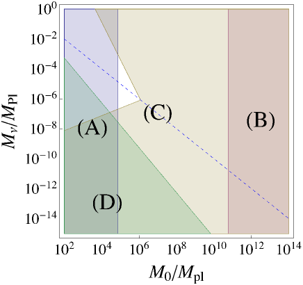
Figure 1: Constraints on the PBH initial mass $M_{0}$ versus the right handed neutrino mass $M_{\nu}$. The region (A) is excluded by the upper bound on the Hubble scale during inflation from the Planck observation (eq. (2.2)). The region (B) is excluded by the condition for the sphaleron process to be effective (eq. (3.8)). The region (C) is excluded by the condition for the enough baryon production from PBHs (eq. (3.6) with $\alpha=1$). In the region (D), the wash out process is effective (eq. (3.7)). The blue dashed line denotes $M_{\nu}=T_{0}$, the boundary of the two cases.

Fig. 1 shows that non-thermal leptogenesis from PBH is possible while the parameter region is restricted by (A) and (C). Consequently, in the PBH leptogenesis scenario, the mass of PBHs and the mass of right-handed neutrino should be in the following region,

$$10^{5}M_{\rm Pl}< M_{0}<10^{6}M_{\rm Pl},$$

$$10^{10}\rm{GeV}< M_{\nu}<10^{15}\rm{GeV}.$$ (3.9)

The restriction to the initial PBH mass eq. (3.9) implies that the inflation scale must be in the range of

$$7\times 10^{12}\rm{GeV}<H_{inf}<7\times 10^{13}\rm{GeV}.$$ (3.10)

Therefore the PBH leptogenesis requires inflation model with large energy scale.

Some comments are in order:

• One may consider that if the first reheating temperature (i.e. the temperature of decay products of inflaton) is larger than $M_{\nu}$, the right handed neutrino is produced not only from PBHs but also from the thermal bath (i.e. thermal leptogenesis), and thus more baryons are generated than we have evaluated. However, the contribution from the thermal bath is negligible since the universe is once dominated by PBHs.

• Although only light PBH masses are allowed (see eq. (3.9)) in the case of type I seesaw model, other lepton violating mechanisms might allow heavier PBHs.

• When we have plotted eq. (3.6), we have set $\alpha=1$. Let us consider the case with $\alpha>1$. It can be seen that as $\alpha$ increases, the condition (3.6) becomes tighter and hence the surviving region in Fig.1 becomes smaller. This is because the entropy production after the PBH evaporation dilutes baryon number from PBHs. Thus for a successful PBH leptogenesis, $\alpha<100$ is required. We will discuss the effect of the entropy production in section 4.4.

4 Dark Matter Production from PBH

4.1 Dark matter production from PBH

In this section, we discuss the possibility of dark matter production from PBHs assuming that there is a stable particle (named DM) in the hidden sector. Then, DMs emitted by the PBH evaporation can be the dark matter which is observed today. In the following, we assume that the interaction of DMs is negligible and its abundance is fixed after the evaporation of PBHs.

The present number density of DMs is estimated in analogy with that of right-handed neutrinos in the previous section,

$$\dfrac{n_{DM}}{s}(t_{\rm now})\simeq 0.4\times\alpha^{-1}N_{\rm DM}\left(\dfrac{M_{0}}{M_{\rm Pl}}\right)^{-5/2}\left(\dfrac{g}{100}\right)^{1/2}\left(\dfrac{g_{*}}{100}\right)^{-1/4},$$ (4.1)

where $N_{\rm DM}$ is the number of DM emitted from one PBH, which is given by

$$N_{DM}\simeq\begin{cases}\dfrac{g_{DM}}{6g}\left(\dfrac{M_{0}}{M_{\rm Pl}}\right)^{2}\quad(M_{\textrm{DM}}<T_{0})\\ \dfrac{g_{DM}}{6g}\left(\dfrac{M_{\textrm{DM}}}{M_{\rm Pl}}\right)^{-2}\quad(M_{\textrm{DM}}>T_{0}),\end{cases}$$ (4.2)

where $g_{\rm DM}$ is the degrees of freedom of DM. Then, the present density parameter of DM is given by

$$\Omega_{\rm DM}=\dfrac{M_{\rm DM}n_{\rm DM}}{\rho_{\rm cri}}\simeq\begin{cases}4\times 10^{5}\alpha^{-1}\left(\dfrac{M_{\rm DM}}{1\text{GeV}}\right)\left(\dfrac{M_{0}}{M_{\rm Pl}}\right)^{-1/2}\quad(M_{\rm DM}<T_{0})\\ 4\times 10^{5}\alpha^{-1}\left(\dfrac{M_{\rm DM}}{1\text{GeV}}\right)^{-1}\left(\dfrac{M_{0}}{M_{\rm Pl}}\right)^{-5/2}\ (M_{\rm DM}>T_{0}),\end{cases}$$ (4.3)

where we set $g=g_{*}=100$ and $g_{\textrm{DM}}=1$.

Therefore consistency with the observed density parameter of dark matter, $\Omega_{DM}\lesssim 0.25$, yields a condition,

$$\begin{cases}\left(\dfrac{M_{\textrm{DM}}}{1\rm{GeV}}\right)\lesssim 7\times 10^{-7}\alpha\left(\dfrac{M_{0}}{M_{\rm Pl}}\right)^{1/2}\quad(M_{\textrm{DM}}<T_{0})\\ \left(\dfrac{M_{\textrm{DM}}}{1\rm{GeV}}\right)\gtrsim(7\times 10^{-7}\alpha)^{-1}\left(\dfrac{M_{0}}{M_{\rm Pl}}\right)^{-5/2}\ (M_{\textrm{DM}}>T_{0}).\end{cases}$$ (4.4)

These conditions strongly restrict the mass of the DM.

4.2 Constraint on warm dark matter

Since the DM is produced non-thermally, we should consider an additional constraint. Dark matters with a high velocity (so-called warm dark matter) are constrained by observations because their free streaming prevent the structure formation in the universe. Let us evaluate the present velocity of DM and compare it with a observational constraint.

First the mean energy of radiated particles from PBHs is approximately given by $6T_{0}=6M_{\rm Pl}^{2}/M_{0}$. Since the momentum is red-shifted by the expansion of the universe, we obtain

$$M_{\rm DM}\,\beta=p(t_{\rm now})=\ \dfrac{a_{\rm evap}}{a_{0}}p(t_{\rm evap})\simeq a_{\rm evap}\times 6\dfrac{M_{\rm Pl}^{2}}{M_{0}},$$ (4.5)

where $a_{0}$ and $a_{\rm evap}$ are the scale factor at the present and at the PBH evaporation time respectively, we set $a_{0}=1$, and $\beta$ is the velocity of DM. Therefore, the DM velocity is evaluated as

$$\beta \simeq\ a_{\rm{evap}}\times 6\left(\dfrac{M_{\textrm{DM}}}{M_{\rm Pl}}\right)^{-1}\left(\dfrac{M_{0}}{M_{\rm Pl}}\right)^{-1}$$

$$\simeq 4\times 10^{-31}\alpha^{-1/3}\left(\dfrac{M_{\textrm{DM}}}{M_{\rm Pl}}\right)^{-1}\left(\dfrac{M_{0}}{M_{\rm Pl}}\right)^{1/2}.$$ (4.6)

Here, we have evaluated $a_{\rm evap}$ as follows. As we have set the present scale factor $a_{0}$ as $1$, the scale factor at the equality time $a_{\rm eq}$ is given by $a_{\rm eq}=\Omega_{\rm r}/\Omega_{\rm m}$, where $\Omega_{\rm r}$ and $\Omega_{\rm m}$ are the present density parameter of the matter and of the radiation respectively. Since the expansion of the universe dilutes the total energy density by the forth power of the scale factor during the radiation dominated stage, $a_{\text{evap}}$ is given by

$$a_{\rm{evap}} =a_{\rm{eq}}\left(\frac{\rho_{\rm{eq}}}{\rho_{\rm{evap}}}\right)^{1/4}\alpha^{-1/3}$$

$$=a_{\rm{eq}}\alpha^{-1/3}\left(\frac{\rho_{\rm{cri}}(a_{0}/a_{\rm{eq}})^{3}}{3M_{\rm Pl}^{2}/(4\tau^{2})}\right)^{1/4}$$

$$\simeq 7\times 10^{-32}\alpha^{-1/3}\left(\dfrac{M_{0}}{M_{\rm Pl}}\right)^{2/3},$$ (4.7)

where $\rho_{\rm eq}$ is the energy density at the equality time and $\rho_{\rm cri}$ is the critical energy density. The dependence on nontrivial $\alpha^{1/3}$ will be explained in section 4.4. For a moment, we set $\alpha=1$. In the third equality we have substituted eq. (2.6) and used observational values of $\rho_{\rm cri},\Omega_{\rm r}$ and $\Omega_{\rm m}$.

The restriction to the present velocity of dark matters is read off from ref. [48] as $\beta<4.9\times 10^{-7}$ . With use of eq. (4.6), we obtain a lower bound on the mass of the DM:

$$\left(\dfrac{M_{\textrm{DM}}}{1\rm{GeV}}\right)\gtrsim 2\times 10^{-6}\alpha^{1/3}\left(\dfrac{M_{0}}{M_{\rm Pl}}\right)^{1/2}.$$ (4.8)

4.3 Result and comments

So far, we have derived two conditions. One is required to obtain the observed dark matter density (eq. (4.4)) and the other comes from the constraint on the warm dark matter (eq. (4.8)). We display these conditions with the restriction on the mass of PBHs, eq. (2.2) in Fig. 2. We also shade the region $M_{\textrm{DM}}>M_{\rm Pl}$, in which we cannot perform a reliable calculation. In the region above/below the dashed lihe, $M_{\rm DM}$ is larger/smaller than the initial Hawking temperature. Note that we have set $\alpha=1$, that is, no entropy production after the PBH evaporation is assumed.

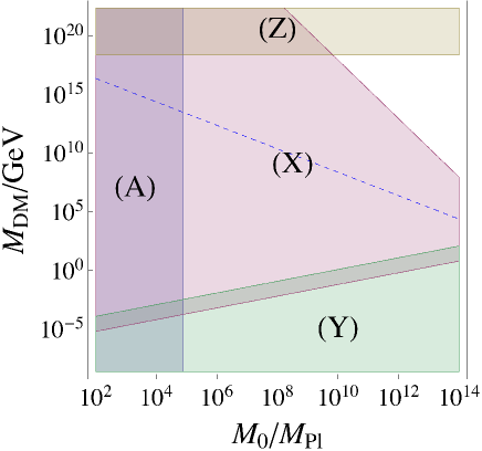
Figure 2: Constraints on the initial PBH mass $M_{0}$ and the DM mass $M_{\rm DM}$. The region (A) is excluded by the constraint on the Hubble scale during inflation from the Planck observation (eq. (2.2)). The region (X) is excluded because $\Omega_{\rm DM}$ exceeds the observed density parameter of the dark matter (eq. (4.4)). On the boundary of (X), the observed dark matter density is obtained. The region (Y) is excluded due to the upper bound on the velocity of dark matters (eq. (4.8)). The region (Z) is shaded because $M_{\textrm{DM}}>M_{\rm Pl}$ and a reliable computation is difficult. The blue dashed line denotes $M_{\textrm{DM}}=T_{0}$, the boundary of the two cases.

We find that the lighter dark matter region (i.e. the region below the (X)) is excluded because of the contradiction with the region (Y). However such a region is allowed if a sufficient entropy production occurs. We discuss the entropy production in the next subsection.

It can also be seen that the upper right region in Fig. 2 is consistent with the observed dark matter density. On the right upper edge of the region (X), the abundance of the observed dark matter density is explained only by DMs emitted from PBHs. There, the mass of the DM is relatively large. Note that this region is incompatible with the generation of baryon asymmetry discussed in the previous section, because the allowed PBH mass regions have no overlap. Therefore PBHs cannot simultaneously produce the right amount of baryon and dark matter without an entropy production.

Let us comment on the compatibility with the grand unified theory (GUT). For $M_{0}\sim 10^{5}M_{\rm Pl}$, which is necessary for a successful PBH leptogenesis, $M_{\textrm{DM}}\sim 10^{15}{\rm GeV}$ is excluded due to the over-closure by the dark matter. In the GUT theory, there is a stable magnetic monopole whose mass is as large as [49]

$$M_{X}/\alpha_{\rm GUT}\sim 10^{16}{\rm GeV}\frac{M_{X}}{10^{15}{\rm GeV}}\left(\frac{\alpha_{\rm GUT}}{1/20}\right)^{-1},$$ (4.9)

where $M_{X}$ is the mass of GUT gauge bosons and $\alpha_{\rm GUT}$ is the fine structure constant of the gauge coupling at the GUT scale. One may wonder that the PBH leptogenesis is incompatible with the GUT. However, the monopole is a topological object and not a fundamental particle. When the radius of the monopole, $M_{X}^{-1}$, is larger than the Schwarzschild radius of PBHs, the emission of monopoles would be suppressed. Monopoles are emitted only for Hawking temperatures smaller than $M_{X}/(4\pi)$, and hence their abundance is suppressed by

$${\rm exp}\left(-\frac{M_{X}/\alpha_{\rm GUT}}{M_{X}/(4\pi)}\right)={\rm exp}\left(-\frac{4\pi}{\alpha_{\rm GUT}}\right)\simeq 10^{-110}~{}~{}(\text{for }\alpha_{\rm GUT}^{-1}=20)$$ (4.10)

in comparison with a fundamental particle. Therefore, the PBH leptogenesis is compatible with the GUT.

4.4 Cogenesis by entropy production

Let us discuss how an entropy production after PBHs evaporate saves the PBH cogenesis scenario. We assume that there exists a matter field (we call it a moduli field) and it dominates the universe after the PBH evaporation. The longer moduli lives, the more entropy is produced when it decays, and more significantly the previous consideration is changed. We show a schematics below:

$$\begin{pmatrix}\text{\rm PBH}\\ \text{evaporation}\\ \end{pmatrix}\xrightarrow[\text{dominant}]{\text{radiation}}\begin{pmatrix}\text{moduli}\\ \text{dominant}\\ \end{pmatrix}\xrightarrow[\text{dominant}]{\text{matter}}\begin{pmatrix}\text{moduli}\\ \text{decay}\\ \end{pmatrix}\xrightarrow[\text{dominant}]{\text{radiation}}\begin{pmatrix}\text{equality}\\ \text{time}\\ \end{pmatrix}$$ (4.11)

Before showing results, we derive the factor $\alpha^{-1/3}$ in eq. (4.7). We start from the equality time and date back to $a_{\rm evap}$ step by step. The scale factor when the moduli decays, $a^{\rm mod}_{\rm dec}$, and that when it dominates the universe, $a^{\rm mod}_{\rm dom}$, are given by

$$a_{\rm dec}^{\rm mod}=a_{\rm{eq}}\left(\dfrac{\rho_{\rm{eq}}}{\rho^{\rm mod}_{\rm dec}}\right)^{1/4},\ a_{\rm dom}^{\rm mod}=a^{\rm mod}_{\rm dec}\left(\dfrac{\rho^{\rm mod}_{\rm dec}}{\rho^{\rm mod}_{\rm dom}}\right)^{1/3},$$ (4.12)

where $\rho^{\rm mod}_{\rm dec}$ and $\rho^{\rm mod}_{\rm dom}$ are the energy density of the universe when the moduli decays and dominates the universe, respectively. Therefore the scale factor when the PBH evaporates $a_{\rm evap}$ is given by

$$a_{\rm{evap}} =a^{\rm mod}_{\rm dom}\left(\dfrac{\rho^{\rm mod}_{\rm dom}}{\rho_{\rm evap}}\right)^{1/4}$$

$$=a_{\rm{eq}}\left(\dfrac{\rho_{\rm{eq}}}{\rho^{\rm mod}_{\rm dec}}\right)^{1/4}\left(\dfrac{\rho^{\rm mod}_{\rm dec}}{\rho^{\rm mod}_{\rm dom}}\right)^{1/3}\left(\dfrac{\rho^{\rm mod}_{\rm dom}}{\rho_{\rm evap}}\right)^{1/4}$$

$$=a_{\rm{eq}}\left(\dfrac{\rho_{\rm{eq}}}{\rho_{\rm evap}}\right)^{1/4}\left(\dfrac{\rho^{\rm mod}_{\rm dec}}{\rho^{\rm mod}_{\rm dom}}\right)^{1/12}$$

$$\simeq a_{\rm eq}\left(\dfrac{\rho_{\rm eq}}{\rho_{\rm evap}}\right)^{1/4}\left(\dfrac{T^{\rm mod}_{\rm dec}}{T^{\rm mod}_{\rm dom}}\right)^{1/3},$$ (4.13)

where $T^{\rm mod}_{\rm dec}$ and $T^{\rm mod}_{\rm dom}$ are the temperature of the universe when the moduli decays and dominates the universe, respectively. In the second equality, we have used eq. (4.12). Let us recall the definition of $\alpha$ and obtain

$$\alpha =\dfrac{s_{\rm{after}}}{s_{\rm{before}}}=\dfrac{4\rho^{\rm mod}_{\rm dec}/(3T^{\rm mod}_{\rm dec})}{\left(a^{\rm mod}_{\rm dec}/a^{\rm mod}_{\rm dom}\right)^{3}s^{\rm mod}_{\rm dom}}$$

$$=\dfrac{{4\rho^{\rm mod}_{\rm dec}/(3T^{\rm mod}_{\rm dec})}}{\left(\rho^{\rm mod}_{\rm dec}/\rho^{\rm mod}_{\rm dom}\right)s^{\rm mod}_{\rm dom}}=\dfrac{4\rho^{\rm mod}_{\rm dom}/(3s^{\rm mod}_{\rm dom})}{T^{\rm mod}_{\rm dec}}$$

$$=T^{\rm mod}_{\rm dom}/T^{\rm mod}_{\rm dec}.$$ (4.14)

Combining eq. (4.12) and eq. (4.13), we obtain eq. (4.7).

Let us consider the effect of the moduli decay. As we have commented in the end of section 3, since the entropy production dilutes the baryon number from PBHs, $\alpha$ has an upper bound $\sim 100$. However, large $\alpha$ dilutes the dark matter emitted from PBHs and relax the restriction from $\Omega_{\rm DM}$ (see eq. (4.4)). Moreover $\alpha$ also changes the evolution of the scale factor and hence the warm dark matter constraint, eq. (4.8). Thus lighter mass regions which are excluded in Fig. 2 is now allowed, if $\alpha$ is larger than $\sim 10$. In conclusion, in the case with

$$10\lesssim\alpha\lesssim 100,$$ (4.15)

the PBH leptogenesis and the dark matter production are compatible with each others. To show this explicitly, we show constraints discussed in the previous section for $\alpha=50$ in Fig. 3.

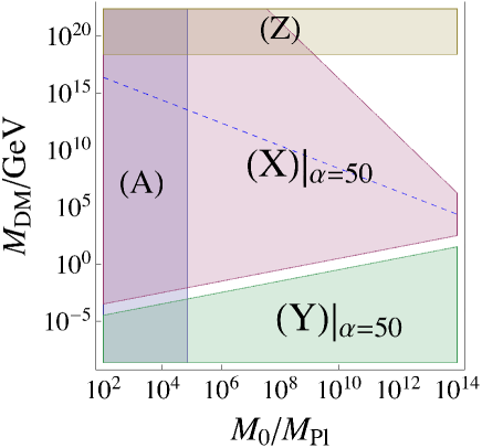
Figure 3: Constrains on the initial PBH mass $M_{0}$ and the DM mass $M_{\rm DM}$ with same constraints with that used on fig. 2 for $\alpha=50$. An allowed region appears between the region (X) and (Y).

We have found that PBHs can be a solution to the coincidence problem. In that case, the model parameters should satisfy

$$M_{0}\sim 10^{5}M_{\rm Pl},\quad M_{\nu}\sim 10^{13}\textrm{GeV},$$

$$\quad M_{\textrm{DM}}\sim 100\textrm{keV},\quad 10\lesssim\alpha\lesssim 100.$$ (4.16)

The restriction to the initial PBH mass $M_{0}\sim 10^{5}M_{\rm Pl}$ implies that the Hubble constant at the inflation is

$$H_{\inf}\gtrsim 10^{13}\rm{GeV}.$$ (4.17)

More precisely, when $\alpha=10$ and eq. (3.6) is almost saturated, $H_{\rm inf}$ is minimized and hence we obtain the lower bound

$$H_{\inf}>2\times 10^{13}{\rm GeV}.$$ (4.18)

This bound can be translated into a lower bound on tensor-to-scalar ratio:

$$r=8\times 10^{-3}\left(\frac{H_{\inf}}{2\times 10^{13}{\rm GeV}}\right)^{2}>8\times 10^{-3}.$$ (4.19)

Thus large field inflation models are favored and gravitational waves generated during inflation will be detected in the near future.

In this section, we have explored the possibility of the cogenesis from PBH with an entropy production by assuming that there is a moduli field. We have always assumed that PBH dominates the universe before it evaporates and $\Omega_{\rm p}$ (the density parameter of the PBH when they are formed) satisfies the condition (2.9). However, if PBHs do not dominate the universe, the cogenesis is also possible. In that case, the condition (3.6) becomes tighter since the baryon number is less produced. At the same time, the condition for dark matter eq. (4.4) becomes relaxed because PBHs produce less dark matters. As a consequence, there comes out a region where leptogenesis and dark matter production work simultaneously as is the case with the entropy production. In both cases, the cogenesis from PBH is realized when the parameters are in the region of eq. (4.16) (for $\Omega_{\rm p}<1$, $\alpha=1$) and thus we will focus on the PBH scenario with such parameters.

5 Generation of Curvature Perturbation from PBH

In this section, we show that PBHs can produce the observed curvature perturbation by the mechanism first proposed in ref. [31]. We show that a local non-gaussianity parameter is bounded from below, $f_{NL}^{\text{local}}>5$. We also discuss an implication to the running of the spectral index.

Before showing detailed calculations, let us briefly explain the basic idea of the mechanism where the fluctuation of PBH evaporation time generates cosmic perturbations. First of all, in the early universe where PBHs dominate, we assume that fermion fields $\psi_{i}$ acquire their masses $m_{\psi,i}$ from a vacuum expectation value (vev) of a light scalar field $\phi$. Then masses $m_{\psi,i}$ are fluctuated if the field value of the light scalar field $\phi$ is also fluctuated by inflation. Secondly, a lifetime of a PBH $\tau$ depends on $m_{\psi,i}$ if $m_{\psi,i}$ are larger than the initial Hawking temperature $T_{0}$ of PBHs. This is because when the Hawking temperature reaches $m_{\psi,i}$, the degrees of freedom of particles emitted from the PBH increases by $g_{f}$, the degrees of freedom of fermion fields $\psi_{i}$, and thus the mass loss rate of the PBH also increases as can be seen from eq. (2.5). Finally, the fluctuation of the PBH evaporation time is nothing but the fluctuation of the (second) reheating time and thus curvature perturbations are generated via the PBH evaporation. A schematic process is illustrated below.

$$\delta\phi\xrightarrow[\text{by vev}]{\text{gives mass}}\delta m_{\psi}\xrightarrow[\text{evaporation}]{\text{PBH }}\delta\tau\xrightarrow[\text{eq.~{}(\ref{deltan})}]{}\delta N=\zeta,$$ (5.1)

where $N$ is an e-folding number and $\zeta$ is a curvature perturbation on the uniform density slice. The fluctuation of $\phi$ generated during inflation is converted successively and finally leads to the curvature perturbation.

In the following, we first derive a relation between the curvature perturbation and the perturbation of the PBH lifetime. Next, we calculate the power spectrum and the non-gaussianity of the curvature perturbation and discuss an implication to the running spectral index. Finally, we discuss constrains on the mass and the decay rate of the scalar field $\phi$.

5.1 $\delta N$ from PBH evaporation

Let us derive a formula for the curvature perturbation when the lifetime of the PBHs, $\tau$, fluctuates, with an aid of the so-called $\delta N$ formula [50, 51, 52].

A flat time slice $t_{i}$ is taken well before PBHs evaporate but well after PBHs dominate the universe as an initial time slice, and a uniform density time slice $t_{f}$ well after the PBH evaporation. A schematic is illustrated below:

$$\begin{pmatrix}\text{initial}\\ \text{time slice}\\ t_{i}\\ \end{pmatrix}\xrightarrow[\text{dominant}]{\text{matter(PBH)}}\begin{pmatrix}\text{\rm PBH}\\ \text{evaporation}\\ \tau\\ \end{pmatrix}\xrightarrow[\text{dominant}]{\text{radiation}}\begin{pmatrix}\text{final}\\ \text{time slice}\\ t_{f}\\ \end{pmatrix}$$ (5.2)

Then, the number of e-foldings between the two slices is given by

$$N=\ln\left[\frac{a(t_{f})}{a(t_{i})}\right]=\ln\left[\left(\dfrac{\tau}{t_{i}}\right)^{2/3}\left(\dfrac{t_{f}}{\tau}\right)^{1/2}\right]=\dfrac{1}{6}\ln\tau+\rm{const.},$$ (5.3)

where $a(t)$ is a scale factor of the universe and we have used a fact that $a(t)$ is proportional to $t^{2/3}$ and $t^{1/2}$ in matter and radiation dominated universe, respectively. A variation of eq. (5.3) yields a relationship between the curvature perturbation and the PBH evaporation time,

$$\zeta=\delta N=\dfrac{1}{6}\dfrac{\delta\tau}{\tau}.$$ (5.4)

From this equation, it is clear that the fluctuation of the PBH evaporation time produces the curvature perturbation.

5.2 Curvature perturbation from fluctuation of the PBH evaporation time

First, let us consider the universe dominated by PBHs. We assume that there are a light scalar field $\phi$, and fermions $\psi_{i}$ which couples with each others via Yukawa interactions

$$\mathcal{L}_{\rm int}=-y_{i}\phi\bar{\psi_{i}}\psi_{i},$$ (5.5)

where $y_{i}$ are yukawa coupling constants. Then the fermion fields obtain a mass from the vev of $\phi$ as

$$m_{\psi,i}=y_{i}\phi.$$ (5.6)

For simplicity, we assume that $m_{\psi,i}=m_{\psi}$, namely all masses are identical.

PBHs lose their masses by emitting particles which are lighter than the Hawking temperature $T$ as we have reviewed in section 2.2. Here, the effective degrees of freedom $g$ is not constant but varies approximately as

$$g=\left\{\begin{array}[]{ll}g_{0}&(T<m_{\psi})\\ g_{0}+g_{f}&(T>m_{\psi})\end{array}\right.,$$ (5.7)

where $g_{0}$ is the total degrees of freedom of particles except fermions $\psi_{i}$, and $g_{f}$ is that of the fermions. If $m_{\psi}$ is larger than the initial Hawking temperature $T_{0}$, one can solve eq. (2.5) as

$$\tau=\tau_{0}\left[1-\xi\left(\frac{T_{0}}{m_{\psi}}\right)^{3}\right],\quad\tau_{0}\equiv\dfrac{160}{\pi g_{0}}\dfrac{M_{0}^{3}}{M_{\rm Pl}^{4}},\quad\xi\equiv\frac{g_{f}}{g_{0}+g_{f}}.$$ (5.8)

Otherwise, i.e. in the case of $m_{\psi}<T_{0}$, $\psi_{i}$ are emitted from the beginning and then $\tau$ does not depend on $m_{\psi}$. The fluctuation of $\phi$ ($\delta\phi$), through Yukawa couplings, induces the fluctuation of the PBH lifetime $\tau$,

$$\delta\tau=3\tau_{0}\xi\left(\frac{T_{0}}{m_{\psi}}\right)^{3}\frac{\delta\phi}{\phi_{\text{evap}}},$$ (5.9)

where $\phi_{\text{evap}}$ is the vev of $\phi$ when PBHs evaporate. Therefore, by using eq. (5.4), we obtain the curvature perturbation,

$$\zeta=\frac{\delta\tau}{6\tau}\simeq\frac{1}{2}\xi\left(\frac{T_{0}}{m_{\psi}}\right)^{3}\frac{\delta\phi}{\phi_{\text{evap}}}.$$ (5.10)

Let us first assume that the mass of $\phi$, $m_{\phi}$, is small enough that $\phi$ does not begin to roll down its potential, that is, $m_{\phi}<\tau_{0}^{-1}$. In this case, the power spectrum of $\delta\phi$ is given by $\mathcal{P}_{\delta\phi}=(H_{\rm inf}/2\pi)^{2}$, and hence the power spectrum of the curvature perturbation is given by

$$\mathcal{P}_{\zeta}^{1/2}=\frac{1}{2}\xi\frac{T_{0}^{3}H_{\inf}/2\pi}{\phi_{\text{evap}}^{4}}y^{-3}\simeq 5\times 10^{-3}\xi\left(\frac{H_{\inf}}{\phi_{\text{evap}}}\right)^{4}y^{-3}.$$ (5.11)

where we have used a relation $T_{0}=H_{\inf}/(4\pi\gamma)$.

If $m_{\phi}>\tau_{0}^{-1}$, $\phi$ begins to oscillate around the minimum of the potential, which we assume to be $\phi=0$. Since the velocity of $\phi$ is large around the minimum while small at the maximum, the mass of fermion fields $\psi_{i}$ is effectively determined by the amplitude of the oscillation. Since the amplitude decreases in proportion to the Hubble scale in the matter dominated universe, the power spectrum of $\delta\phi$ also decreases by $(m_{\phi}\tau_{0})^{-2}\equiv d^{2}$. Hence, their power spectrum of the curvature perturbation is given by

$$\mathcal{P}_{\zeta}^{1/2}\simeq 5\times 10^{-3}\xi\left(\frac{H_{\inf}}{\phi_{\text{evap}}}\right)^{4}y^{-3}d,$$ (5.12)

where $\phi_{\text{evap}}$ is now the amplitude of the oscillation of $\phi$ when PBHs evaporate. In the following, we use the expression (5.12), with $d=1$ for $m_{\phi}<\tau_{0}^{-1}$.

The observed curvature perturbation $\mathcal{P}_{\zeta}^{1/2}\simeq 4.7\times 10^{-5}$ [41] is realized by the evaporation of the PBHs if

$$\phi_{\text{evap}}\simeq 3\times\xi^{1/4}y^{-3/4}d^{1/4}H_{\inf}.$$ (5.13)

5.3 Constraint from $f_{\rm NL}$

Next, let us calculate the non-linear parameter $f_{\rm NL}^{\rm local}$ and argue how the observed value of $f_{\rm NL}^{\rm local}=2.7\pm 5.8$ [41] puts a constraint on our scenario. The local type $f_{\rm NL}^{\text{local}}$ is given by [53]

$$\dfrac{3}{5}f_{\rm NL}^{\text{local}}=3\left(\dfrac{\Gamma^{\prime\prime}}{\Gamma^{\prime 2}}-1\right)=3\left(1-\dfrac{\tau^{\prime\prime}\tau}{\tau^{\prime 2}}\right)$$ (5.14)

where $\Gamma=1/\tau$ is the decay rate of the PBH and ^′ denotes the derivative with respect to the fluctuating field (in our case $\phi$). Using eq. (5.8) and eq. (5.13), we obtain

$$f_{\rm NL}^{\text{local}}=\dfrac{5}{3}\left(2\times 10^{3}\,\xi^{-1/4}\left(yd\right)^{3/4}-1\right).$$ (5.15)

Note that $T_{0}$ must be smaller than $m_{\psi}=y\phi_{\text{evap}}$. Then we obtain a restriction on $\xi$, $y$ and $d$:

$$T_{0}<m_{\psi}\quad\Longrightarrow\quad\xi\left(yd\right)>2\times 10^{-4}.$$ (5.16)

We show constrains on $\xi$, $y$ and $d$ in Fig.4. It can be seen that a suitable region is around $yd\sim 10^{-3},\xi\sim 1$, and that $f_{\rm NL}^{\text{local}}$ is bounded from below, $f_{\rm NL}^{\text{local}}>5$, which is testable by future measurements.

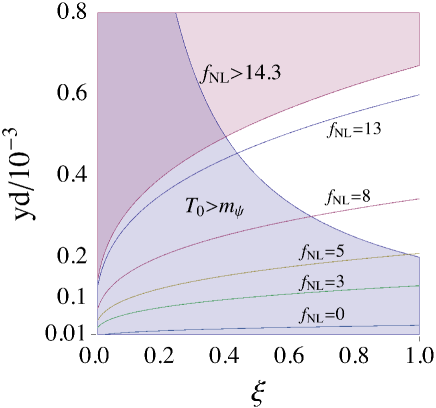
Figure 4: Constraint on $\xi\equiv g_{f}/(g_{0}+g_{f})$, the yukawa coupling $y$ and $d$ from $f_{\rm NL}^{\rm local}$ and the necessary ingredient of our scenario, $m_{\psi}=y\phi_{\text{evap}}>T_{0}$. The blue colored region is excluded since $m_{\psi}>T_{0}$ (eq. (5.16)). Four lines show contours of $f_{\rm NL}^{\text{local}}=13,8,5,3$, from top to bottom (eq. (5.15)). The red colored region is excluded by the observation $f_{NL}^{\text{local}}<14.3$ (95% CL).

5.4 Prediction on the running index

Let us discuss a prediction on the running spectral index assuming the hybrid inflation [54, 55], which can easily yield a blue-tilted spectral [32] and realize the PBH production. We consider the following standard hybrid inflaton potential,

$$V(s)=V_{0}+\frac{1}{2}m_{s}^{2}s^{2}+\cdots,$$ (5.17)

where $s$ is the inflaton and $\cdots$ includes interaction terms with a waterfall sector. With this setup, slow roll parameters are given by

$$\epsilon \equiv\dfrac{M_{\rm Pl}^{2}V^{\prime 2}}{2V^{2}}\simeq\dfrac{m_{s}^{4}M_{\rm Pl}^{2}}{2V_{0}^{2}}s^{2}\ll\eta,$$

$$\eta \equiv\dfrac{M_{pl^{2}}V^{\prime\prime}}{V}\simeq\dfrac{m_{s}^{2}M_{\rm Pl}^{2}}{V_{0}}.$$ (5.18)

The curvature perturbation generated by the inflaton $s$ is

$$\mathcal{P}^{\textrm{inf}}_{\zeta}=\dfrac{V}{24\pi^{2}M_{\rm Pl}^{4}\epsilon}=\dfrac{V_{0}}{12\pi^{2}M_{\rm Pl}^{2}\eta^{2}}s^{-2}.$$ (5.19)

Then, by using eq. (5.18) and eq. (5.19), one can evaluate the number of e-foldings as

$$N_{*}=\dfrac{1}{M_{\rm Pl}}\int_{s_{e}}^{s_{*}}\dfrac{ds}{\sqrt{2\epsilon}}=\dfrac{1}{\eta}\ln\left(\dfrac{s_{*}}{s_{e}}\right)=\dfrac{1}{2\eta}\ln\left(\mathcal{P}^{\textrm{inf}}_{\zeta_{e}}/\mathcal{P}^{\textrm{inf}}_{\zeta_{*}}\right),$$ (5.20)

where we use lower indices $*$ and $e$ to denote that the value is evaluated at the horizon exit of the CMB scale, and the end of the inflation respectively. Recall that the curvature perturbation should be large enough on the small scale in order to produce the PBHs while it it known to be small on the large scale,

$${\cal P}_{\zeta e}^{\rm inf}={\cal O}(1),~{}~{}~{}{\cal P}_{\zeta*}^{\rm inf}\lesssim 10^{-10}.$$ (5.21)

Eq. (5.20) and eq. (5.21) lead to a lower bound on $\eta$ as

$$\eta=\frac{1}{2N_{*}}{\rm ln}\left({\cal P}_{\zeta e}^{\rm inf}/{\cal P}_{\zeta*}^{\rm inf}\right)>0.2\frac{60}{N_{*}},$$ (5.22)

where we have used a relation for the spectral index of the curvature perturbation generated by the inflaton, $n_{s}^{\text{inf}}=1-6\epsilon_{*}+2\eta\simeq 1+2\eta$. This large value of $\eta$ is typical of the supergravity theory [56].

Now let us consider the spectral index of the density perturbation form PBHs, $n_{s}$. Since $\mathcal{P}_{\zeta}\propto\mathcal{P}_{\delta\phi}\propto H_{\rm inf}^{2}$ in eq. (5.12), the spectral index is given by

$$n_{s}=1+\dfrac{d\ln\mathcal{P}_{\zeta}}{dN}=1+\dfrac{d\ln H_{\textrm{inf}}^{2}}{dN}=1-2\epsilon_{*},$$ (5.23)

where we have assumed that the mass of $\phi$, $m_{\phi}$, is far smaller than $H_{\text{inf}}$ and hence does not affect the spectral index. Note that the perturbation is originated from not the inflaton, but the light field $\phi$. In order to obtain the value consistent with the Planck results [41], $n_{s}=0.9607\pm 0.0063$ (95% C.L.),

$$\epsilon_{*}=0.020\pm 0.003$$ (5.24)

is required.

Finally, we show the prediction of the running of the spectral index $n_{s}^{\prime}$,

$$n_{s}^{\prime}=\frac{dn_{s}}{d\ln k}\simeq-4\epsilon_{*}\eta+8\epsilon_{*}^{2}<-0.011\frac{60}{N_{*}},$$ (5.25)

where we used eq. (5.24), and the lower bound of $\eta$ in eq. (5.22). This large value would be tested by future observations.

5.5 Constraint on the scalar field

Finally, we discuss constraints on the mass $m_{\phi}$ and the decay rate $\Gamma_{\phi}$ of $\phi$. We show constraints from the unitarity, the decay after PBHs evaporate, the curvature perturbation generated by $\phi$ as a curvaton [57, 58, 59, 60, 61]. To be concrete, we assume that $\phi$ has a quadratic potential, $V(\phi)=m_{\phi}^{2}\phi^{2}/2$.

Suppose that $\phi$ begins to oscillate before PBHs evaporate. After $\phi$ begins to oscillate, the square amplitude $\phi^{2}$ declines in proportion to $a^{-3}\propto H^{3/2}$ until $\phi$ decays. Thus the amplitude of $\phi$ when it decays $\phi_{\rm dec}$ is given by

$$\phi_{\text{\rm dec}} \simeq\phi_{\rm evap}\left(\Gamma_{\phi}\tau_{0}\right)^{3/4}\simeq\phi_{\rm evap}\left(\frac{\Gamma_{\phi}}{m_{\phi}}\frac{1}{d}\right)^{3/4}$$

$$\simeq 3\times\xi^{1/4}y^{-3/4}d^{-1/2}H_{\inf}\left(\frac{\Gamma_{\phi}}{m_{\phi}}\right)^{3/4}.$$ (5.26)

When $\phi$ begins to oscillate after PBHs evaporate, eq. (5.5) with $d=1$ holds.

As mentioned above, we consider following conditions:

• The unitarity bound on $\Gamma_{\phi}$;

  $$\Gamma_{\phi}<4\pi m_{\phi}.$$ (5.27)

• The unitarity bound on $y$;

  $$y<4\pi,~{}yd\sim 10^{-3}~{}i.e.~{}d=(m_{\phi}\tau_{0})^{-1}>10^{-4}.$$ (5.28)

• $\phi$ must not decay until the end of the PBH evaporation;

  $$\Gamma_{\phi}<1/\tau_{0}\simeq\dfrac{\pi g_{0}}{160}\dfrac{M_{\rm Pl}^{4}}{M_{0}^{3}}\simeq 5\times 10^{3}\rm{GeV}\left(\frac{M_{0}}{10^{5}M_{\rm Pl}}\right)^{-3}.$$ (5.29)

• The curvature perturbation directly generated by $\phi$ as a curvaton must not exceed the observed value;

  $$10^{-5}>\zeta\simeq\dfrac{\delta\rho_{\sigma}}{\rho_{\sigma}}\simeq\dfrac{1}{3}\dfrac{\rho_{\phi_{\rm dec}}}{\rho_{\rm tot}}\dfrac{2(H_{\inf}/2\pi)}{\phi_{\rm evap}}d$$

  $$\simeq 6\times 10^{-8}\left(\frac{M_{0}}{10^{5}M_{\text{Pl}}}\right)^{-2}\left(\frac{m_{\phi}}{\Gamma_{\phi}}\right)^{1/2}\xi^{1/4}\left(\frac{yd}{10^{-3}}\right)^{-3/4}d^{1/2}.$$ (5.30)

In Fig. 5, we show constraints from the above four conditions. Here, we assume that $M_{0}=10^{5}M_{\rm Pl}$ and $yd=10^{-3}$, which is required in our scenario as we have discussed. The colored region is excluded and white region is allowed. Note that since the parameter $d$ is inversely proportional to $m_{\phi}$ for $m_{\phi}>t_{0}^{-1}$, the constraint from the curvature perturbation does not depend on $m_{\phi}$ in that region. It can be seen that much possibilities remain for $m_{\phi}$ and $\Gamma_{\phi}$.

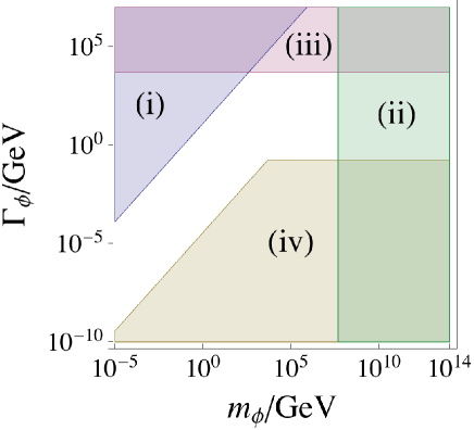
Figure 5: Constraints on $m_{\phi}$ and $\Gamma_{\phi}$. The colored region is excluded due to the conditions (i), (ii), (iii) and (iv).

6 Detectability of Gravitational Waves from PBH

In this section, we discuss the detectability of gravitational waves that are emitted by PBHs. After PBHs evaporate, radiated particles are thermalized and hence no observable signature remains. However, gravitons are exceptional particles because their interactions are so weak that their momentum distribution, namely the spectrum of gravitational waves, maintains information on PBHs. We will calculate the spectrum of gravitons from PBHs and discuss the detectability of the gravitational waves.

6.1 Spectrum of gravitational waves

The spectrum of gravitational waves that are generated by the evaporation of PBHs has been studied in refs. [63, 64]. In ref. [64], the authors analytically obtained the gravitational wave spectrum by assuming an instantaneous evaporation of PBHs and ignoring an increase of the Hawking temperature during the evaporation, while it is taken into account in our calculation. We find that the treatment of ref. [64] does not significantly affect the peak frequency and the peak amplitude of the gravitational waves but the form of the spectrum is altered. A numerical calculation is performed in ref. [63].

Let us compute the spectrum of gravitational waves from the PBH evaporation. Suppose that gravitons emitted with a frequency $\nu\sim\nu+d\nu$ at a time $t$ reach us with a frequency $\nu_{0}$ at the present time $t_{0}$. The relation between $\nu$ and $\nu_{0}$ is

$$\nu=\nu_{0}\dfrac{a(t_{0})}{a(t)}=\dfrac{\nu_{0}}{a(t)},$$ (6.1)

where we have set $a(t_{0})=1$. Remember that the energy spectrum by the Hawking radiation approximately obeys the Planck’s distribution law (see eq. (2.3)) and the energy density of gravitons decreases in proportion to $a^{-4}$. Thus, at $t_{0}$, the energy density of gravitons which is emitted with the frequency $\nu\sim\nu+d\nu$ at the time $t$ is given by

$$d^{2}\rho(t,\nu;t_{0})$$

$$=\dfrac{g_{g}}{g}n_{\rm{\rm PBH}}(t)\times 4\pi r_{s}^{2}\times d^{2}E(t,\nu)\left(\dfrac{a(t)}{a(t_{0})}\right)^{4}$$

$$=\dfrac{\pi g_{g}M(t)^{2}n_{\rm{\rm PBH}}(t)}{2M_{\rm Pl}^{4}}\dfrac{\nu^{3}_{0}d\nu_{0}dt}{\exp(2\pi\nu M(t)/M_{\rm Pl}^{2})-1},$$ (6.2)

where $g_{g}$ is the effective degrees of freedom of graviton, and is assumed to be 1 hereafter [64]. Integrating eq. (6.2) from the PBH formation time $t_{\rm p}$ to the evaporation time $t_{\rm evap}=t_{\rm p}+\tau$, we obtain the present energy density of gravitons with frequency $\nu_{0}\sim\nu_{0}+d\nu_{0}$ as

$$d\rho(\nu_{0})=\int_{t_{\rm p}}^{t_{\rm{evap}}}d^{2}\rho(t,\nu;t_{0})$$

$$=\dfrac{\pi}{2M_{\rm Pl}^{4}}\int_{t_{\rm p}}^{t_{\rm{evap}}}\dfrac{M(t)^{2}n_{\rm{\rm PBH}}(t)}{\exp(2\pi\nu_{0}M(t)/a(t)M_{\rm Pl}^{2})-1}dt\ \nu_{0}^{3}d\nu_{0}.$$ (6.3)

Therefore, the spectral energy density of the gravitational waves is given by

$$\Omega_{\rm{GW}}(\nu_{0})=\dfrac{1}{\rho_{\rm cri}}\dfrac{d\rho(\nu_{0})}{d\ln\nu_{0}}$$

$$=\dfrac{1}{\rho_{\rm cri}}\dfrac{\pi}{2M_{\rm Pl}^{4}}\nu_{0}^{4}\int_{t_{\rm p}}^{t_{\rm evap}}\dfrac{M(t)^{2}n_{\rm PBH}(t)}{\exp\left[2\pi\nu_{0}M(t)/a(t)M_{\rm Pl}^{2}\right]-1}dt,$$ (6.4)

where $\rho_{\rm cri}$ is the present critical density of the universe. The PBH mass $M(t)$ in the integrand is given by

$$M(t)=\left\{\begin{array}[]{ll}M_{0}\left(1-\dfrac{t-t_{p}}{\tau_{L}}\right)^{1/3},&(t_{\rm p}<t<t_{1})\\ M_{1}\left(1-\dfrac{t-t_{p}}{\tau_{H}}\right)^{1/3},&(t_{1}<t<t_{\rm{evap}}),\\ \end{array}\right.$$ (6.7)

$$M_{1}=\frac{M_{{\textrm{Pl}}}^{2}}{m_{\psi}},\ t_{1}=t_{p}+\tau_{L}\left(1-\left(\frac{M_{1}}{M_{0}}\right)^{3}\right)$$

$$\tau_{L}=\dfrac{160}{\pi g_{0}}\dfrac{M_{0}^{3}}{M_{\rm Pl}^{4}},\ \tau_{H}=\dfrac{160}{\pi(g_{0}+g_{f})}\dfrac{M_{1}^{3}}{M_{\rm Pl}^{4}},$$ (6.8)

and the PBH number density $n_{\rm PBH}(t)$ is estimated as

$$n_{\textrm{\rm PBH}}(t)=\left\{\begin{array}[]{ll}n_{\rm PBH}(t_{\rm p})\left(\dfrac{t_{\rm p}}{t}\right)^{3/2}&(t_{\rm p}<t<t_{\rm{dom}}),\\ n_{\textrm{\rm PBH}}(t_{\rm p})\left(\dfrac{t_{\rm p}}{t_{\rm{dom}}}\right)^{3/2}\left(\dfrac{t_{{\rm dom}}}{t}\right)^{2}&(t_{\rm{dom}}<t<t_{\rm{evap}}),\\ \end{array}\right.$$ (6.11)

$$n_{\textrm{\rm PBH}}(t_{\rm p})=\Omega_{\rm p}\dfrac{3M_{\rm Pl}^{2}}{4M_{0}t_{\rm p}^{2}}.$$ (6.12)

In fig. 6, we plot $\Omega_{\rm GW}$ from the PBH evaporation with the allowed parameters discussed in the previous section. We have set $M_{0}=10^{5}M_{\rm Pl},\Omega_{\rm p}=10^{-4}$ and $\alpha=50$. For $\nu_{0}\gtrsim 10^{10}$Hz , $\Omega_{\rm GW}$ does not depend on $\Omega_{\rm p}$ as long as $\Omega_{\rm p}$ is large enough that PBHs dominate the universe before their evaporation (see eq (2.9)). The entropy production changes $a_{\rm evap}$ following eq. (4.7) but it does not affect the spectral form of $\Omega_{\rm GW}$. To be conservative, we have suppressed the contribution of the Hawking radiation whose physical wave number is higher than the Planck scale,

$$k_{\rm phy}(t)\equiv\frac{2\pi\nu_{0}}{a(t)}>M_{\rm Pl}.$$ (6.13)

This is because our semi-classical treatment on the Hawking radiation would not be reliable if energies of radiated particles exceed $M_{\rm Pl}$.

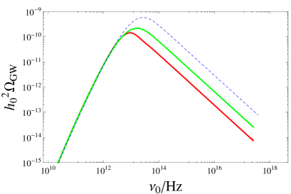
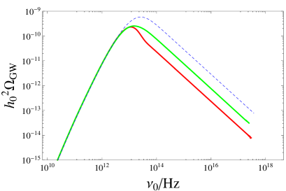
Figure 6: The present spectral energy density of the gravitational waves $\Omega_{\rm GW}(\nu_{0})$ that are generated by the Hawking radiation of PBHs, where $\nu_{0}$ is a current frequency. We have set $M_{0}=10^{5}M_{\rm Pl},\Omega_{\rm p}=10^{-4}$ and $\alpha=50$. The blue dashed, green and red lines represent the cases with $g_{f}=0,\,200,\,900$ (or $\xi=0,\ 2/3,\ 0.9$), respectively. The non-linearity parameters are $f_{\rm NL}=8$ (left panel) and $f_{\rm NL}=13$ (right panel) except for the blue dashed lines which denote the cases without the curvature perturbation production. One can see that $\Omega_{\rm GW}$ decreases as the radiated degrees of freedom $g$ increases because the increase of $g$ reduces the fraction of the emission into gravitational waves.

Lines in fig. 6 have a peak with frequency $\nu_{0}^{\rm peak}\sim 10^{13}$Hz and a cut off with frequency $\nu_{0}^{\rm peak}\sim 10^{18}$Hz . In the next few paragraphs, we discuss the physical understanding of this behavior. We mention the behavior of the blue dashed lines in fig. 6 in which $g_{f}=0$. Effects of non-zero $g_{f}$ will be discussed later.

First, note that the integration in eq. (6.4) has the largest contribution from $\nu\sim T$ because the Hawking radiation is approximated by the black body radiation. For a graviton with $\nu_{0}\lesssim\nu_{0}^{\rm peak}$, its initial frequency is higher than the Hawking temperature, $\nu(t_{\rm p})\gg T(t_{\rm p})$, while this relation is inverted before $t_{\rm evap}$, because $\nu\,(\propto a^{-1})$ decreases due to the cosmic expansion. Thus the physical frequencies of these modes is once as large as $T(t_{\rm p})$ and hence receive contributions mainly from the peak of the Hawking radiation, $\nu\sim T\sim T(t_{\rm p})$. By remembering the time dependence of $n_{\rm PBH}(t)$ and $a(t)$, as well as the integrand in eq. (6.4), $\Omega_{\rm GW}\propto\nu_{0}^{5/2}$ is obtained in this region.

For $\nu_{0}^{\rm peak}\lesssim\nu_{0}\leq\nu_{0}^{\Lambda}$, the Hawking temperature $T$ exceeds $\nu$ just before the evaporation because $T$ increases as the PBH mass decreases. Therefore for these frequencies, the time variation of $\nu$ and $n_{\rm BH}$ are irrelevant but that of $M$ is important. Since $T$ grows faster as $t$ approaches $t_{\rm evap}$, the time duration in which $\nu\sim T$ becomes shorter for higher $\nu$, and thus a smaller contribution of the integration in eq. (6.4) is expected for higher $\nu$. By remembering the time dependence of $M(t)$ and the integrand in eq. (6.4), we obtain $\Omega_{\rm GW}\propto\nu_{0}^{-1}$.

For $\nu_{0}^{\Lambda}<\nu_{0}$, the physical wave number $k_{\rm phy}(\propto a^{-1})$ does not become smaller than $M_{\rm Pl}$ before $t=t_{\rm evap}$. Since we neglect the contributions from the modes with $k_{\rm phy}>M_{\rm Pl}$, these frequencies are not plotted in fig. 6.

Next, let us discuss the effect of the growth of the radiated degrees of freedom $g$. In our scenario, the degrees of freedom radiated by PBHs increases from $g_{0}$ into $g_{0}+g_{f}$ when the Hawking temperature T exceeds $m_{\psi}$ (see eq. (5.7)). Although the emission of gravitons from PBHs is independent of the other degrees of freedom (see eq. (6.2)), it is indirectly affected by $g_{f}$ because the increase of $g$ changes the evolution of the PBH mass $M(t)$. The increase of $g$ accelerates the mass loss of PBHs and hence the time integration in eq. (6.4) declines. In other words, the increase of $g$ reduces the fraction of the emission into gravitational waves. Therefore, for $\nu_{0}^{\rm peak}\lesssim\nu_{0}\leq\nu_{0}^{\Lambda}$ where gravitons are mainly emitted after $T$ begins to grow significantly, $\Omega_{\rm GW}(\nu_{0})$ drops as $g_{f}$ increases. As one see in fig. 6, the graviton emission decreases by a factor of $g_{0}/(g_{0}+g_{f})=1-\xi$ after $g$ increases. If $m_{\psi}$ is larger, the time when $g$ changes becomes later and the frequency in which $\Omega_{\rm GW}$ drops becomes higher. However, provided that $\xi$ is fixed, from eqs. (5.13) and (5.15), one find that $m_{\psi}$ is connected to $f_{\rm NL}^{\rm local}$ as

$$f_{\rm NL}^{\rm local}+\frac{5}{3}\propto m_{\psi}^{3}(t_{\rm evap}).$$ (6.14)

$m_{\psi}$ has an upper bound depending on $\xi$ (as we see in fig. 4) and $m_{\psi}$ can not be much larger than $T_{0}$. Thus the peak amplitude of $\Omega_{\rm GW}$ is inevitably suppressed in comparison to the case with $g_{f}=0$.

$\Omega_{\rm GW}(\nu_{0})$ can be translated into the amplitude of gravitational waves $h(\nu_{0})$. The energy density of the gravitational waves is $\rho_{\textrm{GW}}=\frac{1}{2}M_{\textrm{Pl}}^{2}\nu^{2}h^{2}$, which leads to the relation $\Omega_{\textrm{GW}}=\rho_{\textrm{GW}}/\rho_{\textrm{cri}}=M_{\textrm{Pl}}^{2}\nu^{2}h^{2}/2\rho_{\textrm{cri}}$. Thus the amplitude corresponding to the peak ($\Omega_{\textrm{GW}}\sim 10^{-10},\nu\sim 10^{13}\textrm{Hz}$) is estimated as

$$h\sim 10^{-36}.$$ (6.15)

Although other phenomena like the graviton emission from binary PBHs and the quantum bremsstrahlung of gravitons at PBH collisions are also the sources of gravitational waves, their contributions are negligible compared to the Hawking radiation [64].

6.2 Detectability in future experiment

In the previous subsection, we have shown that the peak of the gravitational wave spectrum reaches $\Omega_{\rm GW}\sim 10^{-10}$ at frequency $\nu\sim 10^{13}$Hz. This frequency is too high to be detected by interferometers. However, it is recently pointed out by refs. [67, 65, 66] that a new kind of detector has a capability of detecting high frequency gravitational waves by using the inverse Gertsenshtein effect [68]. In this section, we review the new detection scheme and discuss the possibility of testing our scenario.

The Gertsenshtein effect (G-effect) is the effect suggested by Gertsenshtein that electromagnetic waves yield gravitational waves in a static magnetic field. This is because cross terms in the energy momentum tensor between the static magnetic field and the electromagnetic fields lead to the quadrupole emission of gravitational waves. Inversely, in a static magnetic field, gravitational waves also induce electromagnetic waves. This is called the inverse Gertsenshtein effect, or the inverse G-effect.

Let us explain the basic idea of the high frequency gravitational wave detection experiment discussed in refs. [67, 65, 66] by considering the schematic set-up illustrated in Fig. 7. The static magnetic field toward y-direction $\vec{B}=B\,\vec{e}_{y}$ is uniformly applied in a region, $z>0$. If a gravitational wave with an amplitude $h$ propagates into the z-direction, the following electromagnetic wave is generated by the inverse Gertsenshtein effect (see Appendix for derivation):

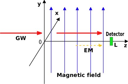
Figure 7: Magnetic field $B$ is applied in the y-direction and a gravitational wave with frequency $\nu_{g}$ , wave number $k_{g}$ and amplitude $h$ propagates into the z-direction. We assume that this system is large enough compared with the wave length, so that the system is considered to be translational symmetric in the x- and the y-direction.

$$\vec{E}^{(1)}(z,t)=E^{(1)}\scalebox{0.9}{$\displaystyle\left(\begin{array}[]{c}\cos\beta\\ \sin\beta\\ 0\end{array}\right)$}\exp[i(k_{g}z-2\pi\nu_{g}t+\delta)],$$ (6.19)

$$\vec{B}^{(1)}(z,t)=\dfrac{1}{c}E^{(1)}\scalebox{0.9}{$\displaystyle\left(\begin{array}[]{c}-\sin\beta\\ \cos\beta\\ 0\end{array}\right)$}\exp[i(k_{g}z-2\pi\nu_{g}t+\delta)],$$ (6.23)

$$E^{(1)}\simeq hBk_{g}cz,$$ (6.24)

where the upper index ⁽¹⁾ means a first-order magnitude in $h$ , $\beta$ denotes the angle between the polarization vector of the electromagnetic wave and the x-axis, and $\delta$ is the initial phase. Note that the induced electromagnetic wave becomes stronger as it propagates, $E^{(1)}\propto z$. The power flux at the detection point $z=L$ is

$$U_{em}^{(2)} \equiv\dfrac{1}{\mu_{0}}\left\langle\left|\vec{E}^{(1)}\times\vec{B}^{(1)}\right|\right\rangle\times A$$

$$=\dfrac{1}{\mu_{0}}B^{2}\times(k_{g}L)^{2}\times c\times h^{2}\times A$$

$$=\dfrac{4\pi^{2}}{c}\dfrac{1}{\mu_{0}}B^{2}L^{2}A\nu_{g}^{2}h^{2},$$ (6.25)

where $A$ is the area of the detector. The flux (i.e. the number of photon per unit time) is

$$n^{(2)} \equiv\dfrac{1}{2\pi\hbar\nu_{g}}U_{em}^{(2)}=\dfrac{2\pi}{c\hbar}\dfrac{1}{\mu_{0}}B^{2}L^{2}A\nu_{g}h^{2}$$

$$=1.8\times 10^{-24}\textrm{s}^{-1}\left(\frac{B}{10^{\textrm{T}}}\right)^{2}\left(\frac{L}{10^{2}\textrm{m}}\right)^{2}\left(\frac{A}{10^{-4}\textrm{m}^{2}}\right)^{2}\left(\frac{\nu_{g}}{10^{13}\textrm{Hz}}\right)\left(\frac{h}{10^{-36}}\right)^{2}.$$ (6.26)

This value is too small to be distinguished from thermal noise.

The reason why $n^{(2)}$ becomes so small is that $n^{(2)}$ is given by the second order in $h$ which is much smaller than unity. Therefore, in refs. [67, 65, 66], a new technique is suggested. If one applies 0-th order electromagnetic waves $(\vec{E}^{(0)},\vec{B}^{(0)})$ as a background, a first order signal flux $n^{(1)}$ appears as follows,

$$\vec{U}_{em}\equiv \dfrac{1}{\mu_{0}}\left\langle(\vec{E}^{(0)}+\vec{E}^{(1)})\times(\vec{B}^{(0)}+\vec{B}^{(1)})\right\rangle\times A,$$

$$\vec{n}\equiv \dfrac{1}{2\pi\hbar\nu_{g}}\vec{U}_{em}=\vec{n}^{(0)}+\vec{n}^{(1)}+\vec{n}^{(2)}.$$ (6.27)

One may afraid that not only the signal $n^{(1)}$ but also the noise (i.e. the Poisson fluctuation of $n^{(0)}$) is magnified. However, by use of optical ingenuities (e.g. a Gaussian beam and a Fractal membrane), one can distinguish $n^{(1)}$ from $n^{(0)}$ [67, 65, 66]. Thus the noise from $n^{(0)}$ is supposed to be negligible and the condition to detect the signal is estimated as

$$n^{(1)}\Delta t>\sqrt{n_{\textrm{th}}\Delta t},$$ (6.28)

where $\Delta t$ is the detection time and $n_{\textrm{th}}$ is the flux of thermal noise. Let us estimate the possible value of $n^{(1)}$. For instance substituting to eq. (59) of ref. [66] the numerical values, $W_{0}=0.05\textrm{m},l_{1}=0,x=0.005\textrm{m},y=0.01\textrm{m},z=100\textrm{m},\omega_{e}=2\pi\nu_{g}=2\pi\times 10^{13}\textrm{Hz}$, and multiplying $A=10^{-4}\textrm{m}^{2}$, we obtain the signal flux as

$$n^{(1)} =400\ \textrm{s}^{-1}\times\scalebox{0.9}{$\displaystyle\left(\frac{h}{10^{-36}}\right)\left(\frac{B}{10\textrm{T}}\right)\left(\frac{\psi_{0}}{1.26\times 10^{3}\textrm{Vm}^{-1}}\right)$},$$ (6.29)

where $\psi_{0}$ is the amplitude of the background Gaussian beam. Therefore, if the thermal noise is sufficiently small, the magnetic field $B$ is enough strong, and/or the detection time is enough long, eq. (6.28) may be satisfied and we can test the existence of evaporating PBHs.

7 Conclusion

In this paper, we have investigated the consistency of a scenario in which dark matters, the baryon asymmetry as well as the cosmic perturbation are generated from PBHs. This scenario can explain the coincidence of the dark matter and the baryon density of the universe, and is free from the isocurvature perturbation problem.

First, we have investigated the possibility of the PBH leptogenesis through emission right-handed neutrinos and their non-thermal decay, and shown that

$$10^{5}M_{\textrm{Pl}}< M_{0}<10^{6}M_{\textrm{Pl}},\quad(\text{i.e. }7\times 10^{12}\textrm{GeV}<H_{\textrm{inf}}<7\times 10^{13}\textrm{GeV})$$

$$10^{10}\textrm{GeV}< M_{\nu}<10^{15}\textrm{GeV}$$ (7.1)

are required.

Next, we have considered the dark matter production from the evaporation of PBHs, assuming a stable particle in hidden sectors. Only heavy dark matter ($M_{\textrm{DM}}\gtrsim 10^{10}\textrm{GeV}$) is allowed by the constraint on warm dark matters, but it is inconsistent with PBH Leptogenesis. If entropy is produced after the PBH evaporation by a factor of $10\sim 100$ due to the domination by some moduli field, the cogenesis (producing baryon number and dark matter of the same order) from PBHs is possible. In that case, the PBH mass is given by

$$M_{0}\sim 10^{5}M_{\textrm{Pl}},\quad$$ (7.2)

and the mass of right-handed neutrinos and dark matter are determined as

$$M_{\nu}\sim 10^{13}\textrm{GeV},\ M_{\textrm{DM}}\sim 100\textrm{keV}.$$ (7.3)

The Hubble scale during inflation is bounded as

$$H_{\inf}>2\times 10^{13}{\rm GeV},$$ (7.4)

and it corresponds to the lower bound on tensor-to-scalar ratio:

$$r>8\times 10^{-3}.$$ (7.5)

Thirdly, a density perturbation from the PBH evaporation has been discussed. We have shown that the observed density perturbation is obtained without contradiction to the above mentioned constraints. We have obtained predictions on the non-Gaussianity (the value of $f_{\textrm{NL}}$) and the running of the spectral index:

$$f_{\textrm{NL}}\gtrsim 5,\quad n_{s}^{\prime}<-0.011\frac{60}{N_{*}}.$$ (7.6)

Finally, we have calculated the spectrum of gravitational waves from the PBHs. The density paramater of gravitational wave $\Omega_{\rm GW}$ and the peak of the spectrum $\nu_{0}^{\rm peak}$ are as large as

$$\Omega_{\rm GW}\sim 10^{-10},~{}~{}\nu_{0}^{\rm peak}\sim 10^{13}~{}{\rm Hz}.$$ (7.7)

Since the frequency of gravitational wave is too high for ongoing interferometers to detect them, we have discussed the possibility of detecting high frequency gravitational waves by future experiments.

Appendix A The inverse G-effect

In this appendix, we briefly review the inverse G-effect [68, 69, 70]. The inverse G-effect is a phenomena that electromagnetic waves are induced by gravitational waves in a static magnetic (or electric) field. It can be understood by following classical calculations. When one considers the usual U(1) gauge symmetric Lagrangian of photon with the minimal coupling to the gravity, $\mathcal{L}=-\sqrt{-g}F_{\mu\nu}F^{\mu\nu}/4$, the Maxwell equations are given by

$$\dfrac{1}{\sqrt{-g}}\partial_{\nu}\left(\sqrt{-g}g^{\mu\alpha}g^{\nu\beta}F_{\alpha\beta}\right) =0,$$ (A.1)

$$\nabla_{\alpha}F_{\mu\nu} =0.$$ (A.2)

Let us consider a perturbation around the Minkowski background,

$$g_{\mu\nu}(x)=\eta_{\mu\nu}+h_{\mu\nu}(x)\ ,\ |h_{\mu\nu}|\ll 1.$$ (A.3)

In the transverse and traceless gauge, gravitational waves are described by two dynamical components of $h_{\mu\nu}$, namely $h_{+}$ and $h_{\times}$ that are defined by

$$h_{\mu\nu}(z,t) =\left(\begin{array}[]{cccc}0&0&0&0\\ 0&+h_{+}&h_{\times}&0\\ 0&h_{\times}&-h_{+}&0\\ 0&0&0&0\end{array}\right),$$ (A.8)

$$h_{+,\times}(z,t) =a_{+,\times}\exp(i(kz-\omega t)),$$ (A.9)

where we have assumed that the gravitational wave moves towards z-direction as plane waves and $a_{+,\times}$ denote the amplitudes of the gravitational waves. In addition, we consider a setup where a static magnetic field, $\vec{B}=B\,\vec{e}_{y}$, uniformly exists in $z>0$, and electromagnetic waves can propagate on it. Provided that the amplitudes of the electromagnetic waves are much smaller than the that of the static magnetic field, the electromagnetic waves can be treated as perturbations

$$F_{\mu\nu}={\small\left(\begin{array}[]{cccc}0&-E^{(0)}_{x}&-E^{(1)}_{y}&-E^{(1)}_{z}\\ E^{(1)}_{x}&0&B^{(1)}_{z}&-(B+B^{(1)}_{y})\\ E^{(1)}_{y}&-B^{(1)}_{z}&0&B^{(1)}_{x}\\ E^{(1)}_{z}&B+B^{(1)}_{y}&-B^{(1)}_{x}&0\end{array}\right)}+\mathcal{O}(h^{2}),$$ (A.14)

where $\vec{E}^{(1)},\vec{B}^{(1)}(\ll B)$ are the first order perturbation of electromagnetic wave. In this background, a careful calculation of eqs. (A.1, A.2) yields the maxwell equations with the gravitational waves,

$$\vec{\nabla}\cdot\vec{E}^{(1)}=0$$ (A.15)

$$\vec{\nabla}\times\vec{B}^{(1)}=\dfrac{1}{c}\partial_{t}\vec{E}^{(1)}+ikB\scalebox{0.9}{$\displaystyle\left(\begin{array}[]{c}a_{+}\\ a_{\times}\\ 0\end{array}\right)$}e^{i(kz-\omega t)}$$ (A.19)

$$\vec{\nabla}\cdot\vec{B}^{(1)}=0$$ (A.20)

$$\vec{\nabla}\times\vec{E}^{(1)}=-\dfrac{1}{c}\partial_{t}\vec{B}^{(1)}.$$ (A.21)

From these equations, we obtain the electromagnetic wave equations with the gravitational waves as

$$\Box\vec{E}^{(1)}(z,t) =k^{2}B\left(\begin{array}[]{c}a_{+}\\ a_{\times}\\ 0\end{array}\right)e^{i(kz-\omega t)},$$ (A.25)

$$\Box\vec{B}^{(1)}(z,t) =k^{2}B\left(\begin{array}[]{c}-a_{\times}\\ a_{+}\\ 0\end{array}\right)e^{i(kz-\omega t)}.$$ (A.29)

One can see that the gravitational waves provide source terms in these wave equations. Solving these equations under a boundary condition

$$\vec{E}^{(1)}(z=0,t)=\vec{B}^{(1)}(z=0,t)=0\ \ (\text{for all}\ t),$$ (A.30)

we obtain the result

$$E_{x}^{(1)} =\frac{Ba_{+}}{2i}kze^{ik(z-ct)}-\frac{Ba_{+}}{2i}\sin(kz)e^{-i\omega t},$$ (A.31)

$$E_{y}^{(1)} =\frac{Ba_{\times}}{2i}kze^{ik(z-ct)}-\frac{Ba_{\times}}{2i}\sin(kz)e^{-i\omega t},$$ (A.32)

$$B_{x}^{(1)} =-\frac{Ba_{\times}}{2i}kze^{ik(z-ct)}+\frac{Ba_{\times}}{2i}\sin(kz)e^{-i\omega t},$$ (A.33)

$$B_{y}^{(1)} =\frac{Ba_{+}}{2i}kze^{ik(z-ct)}+\frac{Ba_{+}}{2i}\sin(kz)e^{-i\omega t}.$$ (A.34)

These solutions express the induction of the electromagnetic waves by the gravitational waves. Their amplitudes are proportional to the amplitude of the static magnetic field and the gravitational waves. The first terms are amplified in proportion to $kz$ because of the continuous energy feeding from the gravitational waves and the uniformity of the static magnetic field. The second terms are negligible in comparison with first terms for $z\gg k^{-1}$.

References

- [1] J. Garcia-Bellido, A. D. Linde and D. Wands, Phys. Rev. D 54, 6040 (1996) [astro-ph/9605094].
- [2] M. Kawasaki, N. Sugiyama and T. Yanagida, Phys. Rev. D 57, 6050 (1998) [hep-ph/9710259].
- [3] J. ’i. Yokoyama, Phys. Rev. D 58, 083510 (1998) [astro-ph/9802357].
- [4] M. Kawasaki, T. Takayama, M. Yamaguchi and J. ’i. Yokoyama, Phys. Rev. D 74, 043525 (2006) [hep-ph/0605271].
- [5] T. Kawaguchi, M. Kawasaki, T. Takayama, M. Yamaguchi and J. ’i. Yokoyama, Mon. Not. Roy. Astron. Soc. 388, 1426 (2008) [arXiv:0711.3886 [astro-ph]].
- [6] K. Kohri, D. H. Lyth and A. Melchiorri, JCAP 0804, 038 (2008) [arXiv:0711.5006 [hep-ph]].
- [7] J. Yokoyama, Astron. Astrophys. 318, 673 (1997) [astro-ph/9509027].
- [8] M. Kawasaki, N. Kitajima and T. T. Yanagida, Phys. Rev. D 87, no. 6, 063519 (2013) [arXiv:1207.2550 [hep-ph]].
- [9] A. Taruya, Phys. Rev. D 59, 103505 (1999) [hep-ph/9812342].
- [10] K. Jedamzik, Phys. Rev. D 55, 5871 (1997) [astro-ph/9605152].
- [11] M. Crawford and D. N. Schramm, Nature 298, 538 (1982).
- [12] S. W. Hawking, I. G. Moss and J. M. Stewart, Phys. Rev. D 26, 2681 (1982).
- [13] H. Kodama, M. Sasaki and K. Sato, Prog. Theor. Phys. 68, 1979 (1982).
- [14] C. J. Hogan, Phys. Lett. B 143, 87 (1984).
- [15] M. Y. Khlopov, Res. Astron. Astrophys. 10, 495 (2010) [arXiv:0801.0116 [astro-ph]].
- [16] B. J. Carr, K. Kohri, Y. Sendouda and J. ’i. Yokoyama, Phys. Rev. D 81, 104019 (2010) [arXiv:0912.5297 [astro-ph.CO]], and references therein.
- [17] B. J. Carr, Astrophys. J. 201, 1 (1975).
- [18] S. W. Hawking, Commun. Math. Phys. 43, 199 (1975) [Erratum-ibid. 46, 206 (1976)].
- [19] D. N. Page, Phys. Rev. D 13, 198 (1976);
- [20] D. N. Page, Phys. Rev. D 14, 3260 (1976).
- [21] D. N. Page, Phys. Rev. D 16, 2402 (1977).
- [22] D. Toussaint, S. B. Treiman, F. Wilczek and A. Zee, Phys. Rev. D 19, 1036 (1979).
- [23] M. S. Turner and D. N. Schramm, Nature 279, 303 (1979).
- [24] M. S. Turner, Phys. Lett. B 89, 155 (1979);
- [25] J. D. Barrow, E. J. Copeland, E. W. Kolb and A. R. Liddle, Phys. Rev. D 43, 984 (1991).
- [26] A. S. Majumdar, P. Das Gupta and R. P. Saxena, Int. J. Mod. Phys. D 4, 517 (1995).
- [27] N. Upadhyay, P. Das Gupta and R. P. Saxena, Phys. Rev. D 60, 063513 (1999) [astro-ph/9903253].
- [28] A. D. Dolgov, P. D. Naselsky and I. D. Novikov, [astro-ph/0009407].
- [29] E. V. Bugaev, M. G. Elbakidze and K. V. Konishchev, Phys. Atom. Nucl. 66, 476 (2003) [Yad. Fiz. 66, 504 (2003)] [astro-ph/0110660].
- [30] D. Baumann, P. J. Steinhardt and N. Turok, hep-th/0703250 [HEP-TH].
- [31] T. Fujita, K. Harigaya and M. Kawasaki, arXiv:1306.6437 [astro-ph.CO].
- [32] J. Garcia-Bellido and A. D. Linde, Phys. Lett. B 398, 18 (1997) [astro-ph/9612141].
- [33] M. Fukugita and T. Yanagida, Phys. Lett. B 174, 45 (1986).
- [34] Y. B. Zel’dovich and I. D. Novikov, Astron. Zh. 43, 758 (1966); Sov. Astronomy 10, 602 (1967).
- [35] S. Hawking, Mon. Not. Roy. Astron. Soc. 152, 75 (1971).
- [36] Nadezhin D.K., Novikov I.D. and Polnarev A. G. 1978 Astron.Zh. 55 216 [Sov.Astron. 22(2) 129 (1978)].
- [37] Shibata M. and Sasaki M. 1999 Phys.Rev.D 60 084002;
- [38] I. Musco and J. C. Miller, arXiv:1201.2379 [gr-qc].
- [39] T. Harada, C. -M. Yoo and K. Kohri, Phys. Rev. D 88, 084051 (2013) [arXiv:1309.4201 [astro-ph.CO]].
- [40] T. Nakama, T. Harada, A. G. Polnarev and J. ’i. Yokoyama, arXiv:1310.3007 [gr-qc].
- [41] P. A. R. Ade et al. [Planck Collaboration], arXiv:1303.5076 [astro-ph.CO]; P. A. R. Ade et al. [Planck Collaboration], arXiv:1303.5082 [astro-ph.CO].
- [42] S. Davidson and S. Sarkar, JHEP 0011, 012 (2000) [hep-ph/0009078].
- [43] K. Harigaya and K. Mukaida, arXiv:1312.3097 [hep-ph].
- [44] V. A. Kuzmin, V. A. Rubakov and M. E. Shaposhnikov, Phys. Lett. B 155, 36 (1985).
- [45] W. Buchmuller, P. Di Bari and M. Plumacher, Nucl. Phys. B 643, 367 (2002) [Erratum-ibid. B 793, 362 (2008)] [hep-ph/0205349].
- [46] M. Flanz, E. A. Paschos, U. Sarkar and J. Weiss, Phys. Lett. B 389, 693 (1996) [hep-ph/9607310].
- [47] A. Pilaftsis, Phys. Rev. D 56, 5431 (1997) [hep-ph/9707235].
- [48] M. Viel, J. Lesgourgues, M. G. Haehnelt, S. Matarrese and A. Riotto, Phys. Rev. D 71, 063534 (2005) [astro-ph/0501562].
- [49] G. ’t Hooft, Nucl. Phys. B 79, 276 (1974).
- [50] M. Sasaki and E. D. Stewart, Prog. Theor. Phys. 95, 71 (1996) [astro-ph/9507001];
- [51] D. Wands, K. A. Malik, D. H. Lyth and A. R. Liddle, Phys. Rev. D 62, 043527 (2000) [astro-ph/0003278];
- [52] D. H. Lyth, K. A. Malik and M. Sasaki, JCAP 0505, 004 (2005) [astro-ph/0411220].
- [53] M. Zaldarriaga, Phys. Rev. D 69, 043508 (2004) [astro-ph/0306006].
- [54] A. D. Linde, Phys. Lett. B 259, 38 (1991).
- [55] A. D. Linde, Phys. Rev. D 49, 748 (1994) [astro-ph/9307002].
- [56] B. A. Ovrut and P. J. Steinhardt, Phys. Lett. B 133, 161 (1983).
- [57] S. Mollerach, Phys. Rev. D 42, 313 (1990).
- [58] A. D. Linde and V. F. Mukhanov, Phys. Rev. D 56, 535 (1997) [astro-ph/9610219].
- [59] K. Enqvist and M. S. Sloth, Nucl. Phys. B 626, 395 (2002) [hep-ph/0109214].
- [60] D. H. Lyth and D. Wands, Phys. Lett. B 524, 5 (2002) [hep-ph/0110002].
- [61] T. Moroi and T. Takahashi, Phys. Rev. D 66, 063501 (2002) [hep-ph/0206026].
- [62] K. Harigaya, M. Ibe, M. Kawasaki and T. T. Yanagida, Phys. Rev. D 87, no. 6, 063514 (2013) [arXiv:1211.3535 [hep-ph]].
- [63] R. Anantua, R. Easther and J. T. Giblin, Phys. Rev. Lett. 103, 111303 (2009) [arXiv:0812.0825 [astro-ph]].
- [64] A. D. Dolgov and D. Ejlli, Phys. Rev. D 84, 024028 (2011) [arXiv:1105.2303 [astro-ph.CO]].
- [65] F. Li, N. Yang, Z. Fang, R. M. L. Baker, Jr., G. V. Stephenson and H. Wen, Phys. Rev. D 80, 064013 (2009) [arXiv:0909.4118 [gr-qc]].
- [66] F. Li, R. M. L. Baker, Jr., Z. Fang, G. V. Stephenson and Z. Chen, Eur. Phys. J. C 56, 407 (2008) [arXiv:0806.1989 [gr-qc]].
- [67] A. M. Cruise, Class. Quant. Grav. 29, 095003 (2012).
- [68] M.E. Gertsenshtein, Sov. Phys. JETP 14, 84 (1962).
- [69] D. Boccaletti et al., Nuovo Cimento B 70, 129 (1970).
- [70] W. K. De Logi and A. R. Mickelson, Phys. Rev. D 16, 2915 (1977).
- [71] Y. .B. Zeldovich and I. D. Novikov, Chicago, Usa: Chicago Univ. ( 1983) 718p
- [72] M. S. Pshirkov and D. Baskaran, Phys. Rev. D 80, 042002 (2009) [arXiv:0903.4160 [gr-qc]].
- [73] A. D. Dolgov and D. Ejlli, JCAP 1212, 003 (2012) [arXiv:1211.0500 [gr-qc]].
- [74] P. Chen and T. Suyama, arXiv:1309.0537 [astro-ph.CO].