A Parameterized Complexity Analysis of Bi-level Optimisation with Evolutionary Algorithms

Abstract

Bi-level optimisation problems have gained increasing interest in the field of combinatorial optimisation in recent years. With this paper, we start the runtime analysis of evolutionary algorithms for bi-level optimisation problems. We examine two NP-hard problems, the generalised minimum spanning tree problem (GMST), and the generalised travelling salesman problem (GTSP) in the context of parameterised complexity.

For the generalised minimum spanning tree problem, we analyse the two approaches presented by Hu and Raidl, (2012) with respect to the number of clusters that distinguish each other by the chosen representation of possible solutions. Our results show that a (1+1) EA working with the spanning nodes representation is not a fixed-parameter evolutionary algorithm for the problem, whereas the global structure representation enables to solve the problem in fixed-parameter time. We present hard instances for each approach and show that the two approaches are highly complementary by proving that they solve each other’s hard instances very efficiently.

For the generalised travelling salesman problem, we analyse the problem with respect to the number of clusters in the problem instance. Our results show that a (1+1) EA working with the global structure representation is a fixed-parameter evolutionary algorithm for the problem.

1 Introduction

Many interesting combinatorial optimisation problems are hard to solve and meta-heuristic approaches such as local search, simulated annealing, evolutionary algorithms, and ant colony optimisation have been used for a wide range of these problems.

In recent years, researchers became very interested in bi-level optimisation for single-objective (Koh,, 2007; Legillon et al.,, 2012) and multi-objective problems (Deb and Sinha,, 2009, 2010). Such problems can be split up into an upper and a lower level problem which depend on each other. By fixing a possible solution for the upper level problem, the lower level is optimised with respect to the given objective and the constraints imposed by the choice of the upper level.

Recently, Hu and Raidl (Hu and Raidl,, 2011, 2012) have proposed two different approaches for the generalised minimum spanning tree problem (GMSTP). Both approaches work with an upper layer and a lower layer solution. The upper layer solution $x$ is evolved by an evolutionary algorithm whereas the optimal solution $y$ of the lower layer problem corresponding to a particular search point $x$ of the upper layer can be found in polynomial time using deterministic algorithms.

Our goal is to understand the two different approaches by parameterised computational complexity analysis (Downey and Fellows,, 1999). The computational complexity analysis of meta-heuristics plays a major role in the theoretical analysis of this type of algorithms and studies the runtime behaviour with respect to the size of the given input. We refer the reader to (Auger and Doerr,, 2011; Neumann and Witt,, 2010) for a comprehensive presentation. Parameterised complexity analysis takes into account the runtime of algorithms in dependence of an additional parameter which measures the hardness of a given instance. This allows us to understand which parameters of a given NP-hard optimization problem make it hard or easy to be optimised by heuristic search methods. In the context of evolutionary algorithms, the term fixed-parameter evolutionary algorithms has been defined in (Kratsch and Neumann,, 2013). An evolutionary algorithm is called a fixed-parameter evolutionary algorithm for a given parameter $k$ iff its expected runtime is bounded by $f(k)\cdot\operatorname{poly}(n)$ where $f(k)$ with respect to the input size $n$. Parameterised computational complexity analysis of evolutionary algorithms have been carried out for the vertex cover problem (Kratsch and Neumann,, 2013), the computation of maximum leaf spanning trees (Kratsch et al.,, 2010), makespan scheduling (Sutton and Neumann, 2012b, ), and the travelling salesperson problem (Sutton and Neumann, 2012a, ).

We push forward the parameterised analysis of evolutionary algorithms and present the first analysis in the context of bi-level optimization. In our investigations, we take into account the two NP-hard problems the generalised minimum spanning tree problem (GMSTP) and the generalised travelling salesman problem (GTSP) which share the parameter, number of clusters $m$. We consider two different bi-level representations for GMTSP which both have a polynomially solvable lower level part. For the Spanning Nodes Representation, we present worst case examples which show that there are instances leading to an optimization time of $\Omega(n^{m})$. For the Global Structure Representation, we show that it leads to a fixed-parameter evolutionary algorithm with respect to the number of clusters $m$. Furthermore, we present an instance class where the algorithm using the Global Structure Representation encounters an optimization time of $m^{\Omega(m)}$. Analysing both approaches on each others worst-case instances, we show that they solve them very efficiently. This shows the complementary abilities of these two representations for the GMSTP. Then we extend our results for Global Structure Representation to GTSP to show that a similar algorithm has an expected optimisation time of $m^{\Omega(m)}$ for this problem as well.

The paper is divided into two main parts according to the two different problems. The first part (based on the conference version (Corus et al.,, 2013)) where the GMSTP problem is investigated is presented in Section 2. We show hard instances for the Spanning Nodes Representation in Section 2.2 and show that a simple evolutionary algorithms needs exponential time even if the number of clusters is small. In Section 2.3, we examine the Global Structure Representation and show that this leads to fixed-parameter evolutionary algorithms for GMSTP. We point out complementary abilities in Section 2.4. This article extends the conference version (Corus et al.,, 2013) by investigations of the GTSP and some generalizations. We examine the GTSP problem with the corresponding Global Structure Representation in Section 3 and provide upper and lower bounds on the optimisation time of the considered algorithm. Furthermore, we point out in Section 4 general characteristics which allows this fixed-parameter result to be extended to other problems.

2 Generalised Minimum Spanning Tree Problem

In this section, we consider the GMSTP problem and provide the runtime analysis with respect to bi-level representations given in (Hu and Raidl,, 2011, 2012).

2.1 Preliminaries

We consider the generalised minimum spanning tree problem (GMSTP) introduced in (Myung et al.,, 1995). The input is given by an undirected complete graph $G=(V,E,c)$ on $n$ nodes with a cost function $c\colon E\rightarrow\mathds{R}_{+}$ that assigns positive costs to the edges. Furthermore, a partitioning of the node set $V$ into $m$ pairwise disjoint clusters $V_{1},V_{2},\ldots,V_{m}$ is given such that $n=\sum_{i=1}^{m}\left|{V_{i}}\right|$.

A solution to the GMSTP problem consists of two components, the $m$ chosen nodes $P$, called the spanning nodes, in the $m$ clusters, and a minimum spanning tree $T$ on the graph induced by the spanned nodes. More precisely, a solution $S=(P,T)$ consists of a node set $P=(p_{1},\ldots,p_{m})\in V^{m}$, where $V^{m}=V_{1}\times V_{2}\times\cdots\times V_{m}$ and a spanning tree $T\subseteq E$ on the subgraph $G[P]=G(P,\{e\in E\mid e\subseteq P\})$ induced by $P$. The cost of $T$ is the cost of the edges in $T$, i. e.,

$$C(T)=\sum_{(u,v)\in T}c(u,v).$$

The goal is to compute a solution $S^{*}=(P^{*},T^{*})$ which has minimal cost among all possible solutions $S=(P,T)$. For an easier presentation, we assume in some cases that edge costs can be $\infty$. In this case, we restrict our investigations to solutions that do not include edges with cost $\infty$. Alternatively, one might view this as the GMSTP defined on a graph that is not necessarily complete.

The GMSTP problem is NP-hard (Myung et al.,, 1995) and two different bi-level evolutionary approaches have been examined in (Hu and Raidl,, 2012). The first approach presented in (Hu and Raidl,, 2012) uses the Spanned Nodes Representation. It selects in the upper level problem a node for each cluster and computes on the lower level a minimum spanning tree (using for example Kruskal’s algorithm in time $O(m\log m)$) on the induced subgraph.

The second approach uses the Global Structure Representation. It constructs a complete graph $H=(V^{\prime},E^{\prime})$ from the given input graph $G=(V,E,c)$ and the set of pair-wise disjoint clusters $V_{1},V_{2},\ldots,V_{m}$. The node $v_{i}\in V^{\prime}$, $1\leq i\leq m$, corresponds to the cluster $V_{i}$ in $G$. The search space for the upper level consists of all spanning trees of $H$ and the spanned nodes of the different clusters are selected in time $O(n^{2})$ using the dynamic programming approach of Pop (Pop,, 2004).

For our theoretical investigations, we measure the runtime of the algorithms by the number of fitness evaluations required to obtain an optimal solution. We call this the optimization time of the examined algorithm. The expected optimization time refers to the expected number of fitness evaluations until an optimal solution has been obtained for the first time.

2.2 Spanned Nodes Representation

We analyse the cluster based (1+1) EA in this section. Our first theorem shows that this algorithm is an XP-algorithm (Downey and Fellows,, 1999), i. e. an algorithm that runs in time $O(n^{g(m)})$ where $g(m)$ is a computable function only depending on $m$, when choosing the number of clusters $m$ as a parameter.

Theorem 1.

For any instance of the GMSTP problem, the expected time until the cluster based (1+1) EA reaches the optimal solution is $O(n^{m})$.

Proof.

For any search point $x$, let $w(x)\in[m]$ denote the number of clusters where the spanned node representation includes a suboptimal node. If the algorithm chooses all $w(x)$ suboptimal clusters for mutation and selects the optimal node in each of them, then the optimal solution is obtained. Since $w(x)\leq m$, the probability that all suboptimal clusters are mutated in a single step is at least $(1/m)^{m}$. The probability of choosing the optimal node in cluster $i$ is $1/|V_{i}|$. Thus, the probability of jumping to the optimal solution from any search point is at least

$$(m)^{-m}\prod_{i=1}^{m}|V_{i}|^{-1}.$$

Since $\sum_{i=1}^{m}V_{i}=n$, it holds that

$$\prod_{i=1}^{m}\frac{1}{|V_{i}|}\geq(m/n)^{m}.$$

Therefore, the probability of reaching the optimal solution in one step is $\Omega(n^{-m})$, and the expected time to reach the optimal solution is bounded from above by $O(n^{m})$. ∎

We now consider an instance of GMSTP which is difficult for the cluster based (1+1) EA. The hard instance $G_{S}$ for the Spanning Nodes Representation is illustrated in Figure 1. It consists of $m$ clusters, where one cluster is called the central cluster, and the $m-1$ other clusters are called peripheral clusters. Each cluster contains $n/m$ nodes and we assume that $n=m^{2}$ holds. The nodes in the peripheral clusters are called peripheral nodes, and the nodes in the central cluster are called central nodes. Within each cluster, one of the nodes is called optimal, and is marked black in the figure. The remaining $(n/m)-1$ nodes are called sub-optimal nodes, and are marked white in the figure. The instance is a bi-partite graph, where edges connect peripheral nodes to central nodes. The cost of any edge between two optimal nodes is 1, the cost of any edge between two suboptimal nodes is 2. The cost of any edge between a suboptimal peripheral node and the optimal central node is $n^{2}$, and the cost of any edge between an optimal peripheral node and a suboptimal central node is $n$. A cluster is called optimal in a solution, if the solution has chosen the optimal node in that cluster.

Figure 1: Hard instance $G_{S}$ for Spanning Node Representation.

Theorem 2.

Starting with an initial solution chosen uniformly at random, the expected optimization time of the cluster based (1+1) EA on $G_{S}$ is $\Omega(n^{m})$.

Furthermore, for any constant $\epsilon>0$, the probability of having obtained an optimal solution after at most $n^{(1-\epsilon)m}$ iterations is $e^{-\Omega(m)}$.

Proof.

We define two phases for the run of the (1+1) EA. The first phase consists of the first $n-1$ iterations while the second phase starts at the end of the first phase and continues for $n^{m/12}$ iterations. Four distinct events are considered failures during the run of the (1+1) EA for the instance described above.

1. The first failure occurs if during the first phase of the run, the algorithm obtains a search point with less than $m/6$ sub-optimal peripheral clusters.

2. The second type of failure occurs when the central cluster fails to switch to a suboptimal node at least once during the first phase.

3. The third type of failure occurs when the algorithm does not switch all the optimal peripheral clusters to suboptimal clusters during the second phase.

4. The fourth failure corresponds to a direct jump to the optimal solution during the second phase.

We first show that the probability of the first failure event is at most $\exp(-\frac{m}{12})$. This implies that with overwhelmingly high probability, a constant fraction of peripheral clusters is always suboptimal during the first $n-1$ iterations. For $i\in[m-1]$ and $t\geq 0$, let $Z_{i}(t),$ be a random variable such that $Z_{i}(t)=1$ if cluster $V_{i}$ is always sub-optimal in iteration 0 through iteration $t$, and $Z_{i}(t)=0$ otherwise. The probability that a suboptimal node is selected in the initial solution is $1-m/n$. In the following iterations, the probability that a cluster is selected for mutation and that its new spanned node is optimal is $(1/m)(m/n)=1/n$. So it is clear that

$$\Pr\left(Z_{i}(t)=1\right)\geq(1-m/n)(1-1/n)^{t}.$$

By linearity of expectation,

$$\mathbf{E}\left[\sum_{i=1}^{m-1}Z_{i}(t)\right]\geq(m-1)\left(1-\frac{m}{n}\right)\left(1-\frac{1}{n}\right)^{t}.$$

Considering a phase length of $t=n-1$, and assuming that $m$ is sufficiently large and $n=m^{2}$ holds, we get

$$\mathbf{E}\left[\sum_{i=1}^{m-1}Z_{i}(t)\right]\geq\frac{m}{3}.$$

Finally, a Chernoff bound (Motwani and Raghavan,, 1995) implies that

$$\Pr\left(\sum_{i=1}^{m-1}Z_{i}(t)\leq\left(1-\frac{1}{2}\right)\frac{m}{3}\right)\leq\exp\left(-m/12\right).$$

We then show that the probability of the second failure event is $\exp(-\Omega(\sqrt{n}))$. In each iteration the probability to switch the central cluster to a suboptimal node is at least

$$p=\frac{1}{m}\left(1-\frac{m}{n}\right)=\Omega\left(\frac{1}{\sqrt{n}}\right).$$

The probability that this event does not occur in $n-1$ steps is

$$(1-p)^{n-1} =\left((1-p)^{1/p}\right)^{(n-1)p}$$

$$\leq\exp(-p(n-1))=\exp(-\Omega(\sqrt{n})).$$

Now, we show that the probability of the third failure event is less than $n^{-m/12}$, assuming that the first two failure events do not occur. As long as the central cluster remains suboptimal, switching a suboptimal node in a peripheral cluster to an optimal node will result in an extra cost of $n-2$. Conversely, switching an optimal peripheral cluster into a sub-optimal cluster will decrease the cost by $n-2$. As long as there is at least one suboptimal peripheral cluster, making the central cluster optimal will incur an extra cost of at least $n^{2}-2$. So, during phase two, the algorithm can not make any suboptimal cluster optimal unless all suboptimal clusters are made optimal in the same iteration. The probability of making at least $m/6$ suboptimal peripheral clusters optimal simultaneously is at most

$$\left(\frac{1}{m}\cdot\frac{m}{n}\right)^{m/6}=\left(\frac{1}{n}\right)^{m/6}.$$

Since the probability to jump to the optimal solution is at most $n^{-m/6}$ in each iteration, it holds by the union bound that the probability of failure event three is at most

$$n^{-m/6}n^{m/12}=n^{-m/12}.$$

Finally, we show that the probability of failure event four is $O(n^{-m/13})$. The probability that an optimal peripheral cluster is made suboptimal by the (1+1) EA is at least

$$\frac{1}{m}\cdot\frac{n-m}{n}\cdot\left(1-\frac{1}{m}\right)^{m-1}\geq\frac{1}{3m}.$$

The expected time $E[T^{sub}]$ until all peripheral clusters have become suboptimal is therefore at most $m\cdot 3m=O(m^{2})$. Considering a phase of length $n^{m/12}$ and taking into account $m^{2}=n$, it holds by Markov’s inequality that the probability of a type four failure is

$$\Pr\left(T^{sub}>n^{m/12}\right)\leq O(m^{2})n^{-m/12}=O({n^{-m/12+4}}).$$

By union bound, the probability that any type of failure occurs is less than the sum of their independent probabilities, which is $e^{-\Omega(m)}$. Hence, with overwhelmingly high probability, after the second phase, the algorithm has obtained a locally optimal solution where all peripheral clusters are sub-optimal. After that iteration, the probability to jump directly to the optimal solution is $n^{-m}$, and the expected time for this event to occur is $n^{m}$.

Let $E$ be the event that no failure occurs. Then, the first statement of the theorem follows by the law of the total probability,

$$\mathbf{E}\left[T\right] \geq\mathbf{E}\left[T|E\right]\Pr\left(E\right)$$

$$=\Omega(n^{m})(1-e^{-\Omega(m)})$$

$$=\Omega(n^{m}).$$

Furthermore, by union bound, it holds that

$$\Pr\left(T<n^{(1-\epsilon)m}\mid E\right)\leq n^{(1-\epsilon)m}n^{-m}=n^{-\epsilon m}.$$

Hence, the second statement of the theorem follows by the law of total probability

$$\Pr\left(T<n^{(1-\epsilon)m}\right) =\Pr\left(T<n^{(1-\epsilon)m}\mid E\right)\Pr\left(E\right)$$

$$\quad+\Pr\left(T<n^{(1-\epsilon)m}\mid\overline{E}\right)\Pr\left(\overline{E}\right)$$

$$\leq\Pr\left(T<n^{(1-\epsilon)m}\mid E\right)+\Pr\left(\overline{E}\right)$$

$$\leq n^{-\epsilon m}+e^{-\Omega(m)}=e^{-\Omega(m)}.$$

∎

Our results for the Spanned Nodes Representation show that the cluster based (1+1) EA obtains an optimal solution in time $O(n^{m})$ and our analysis for the hard instance $G_{S}$ shows that this bound is tight.

2.3 Global Structure Representation

The second approach examined in (Hu and Raidl,, 2012) uses the Global Structure Representation. It works on the complete graph $H=(V^{\prime},E^{\prime})$ obtained from the input graph $G=(V,E,c)$. The node $v_{i}\in V^{\prime}$, $1\leq i\leq m$, represents the cluster $V_{i}$ of $G$.

The upper level solution in the Global Structure Representation is a spanning tree $T$ of $H$ and the lower level solution is a set of nodes $P=(p_{1},\ldots,p_{m})$ with $p_{i}\in V_{i}$ that minimises the cost of a spanning tree which connects the clusters in the same way as $T$. Given a spanning tree $T$ of $H$, the set of nodes $P$ can be computed in time $O(n^{2})$ using dynamic programming (Pop,, 2004).

We consider the tree based (1+1) EA outlined in Algorithm 1. It starts with a spanning tree $T$ of $H$ that is chosen uniformly at random. In each iteration, a new solution $T^{\prime}$ of the upper layer is obtained by performing $K$ edge-swaps to $T$. Here the parameter $K$ is chosen according to the Poisson distribution with expectation $1$. In one edge swap, an edge $e$ currently not present in the solution is introduced and an edge from the resulting cycle is removed such that a new spanning tree of $H$ is obtained. After having produced the offspring $T^{\prime}$, the corresponding set of nodes $P^{\prime}$ is computed using dynamic programming. $P$ and $T$ are replaced by $P^{\prime}$ and $T^{\prime}$ if the cost of the new solution is not worse than the cost of the old one.

Algorithm 1 Tree based (1+1) EA

  Choose a spanning tree $T$ of $H$.

  Apply dynamic programming to find the minimum spanned nodes $P=(p_{1},\ldots,p_{m})$ induced by $T$.

  while termination condition not satisfied do

     $T^{\prime}\leftarrow T$

     for $i\in\left[K\right]$ where $K\sim\operatorname{Pois}(1)$ do

         Sample edge $e\sim\operatorname{Unif}\left(E^{\prime}\setminus T\right)$

         Sample edge $e^{\prime}\sim\operatorname{Unif}$(edges in cycle in $T^{\prime}\cup\left\{e\right\}$)

         $T^{\prime}\leftarrow T^{\prime}\cup\{e\}\setminus\left\{e^{\prime}\right\}$

     end for

     Apply dynamic programming to find a set of spanned nodes $P^{\prime}=(p^{\prime}_{1},\ldots,p^{\prime}_{m})$ with respect to $T^{\prime}$ of minimal cost.

     if $\sum_{(i,j)\in T^{\prime}}c(p^{\prime}_{i},p^{\prime}_{j})\leq\sum_{(i,j)\in T}c(p_{i},p_{j})$ then

        $P\leftarrow P^{\prime}$

        $T\leftarrow T^{\prime}$

     end if

  end while

In the following, we show that the tree based (1+1) EA is a fixed-parameter evolutionary algorithm for the GMSTP problem when considering the number of clusters $m$ as the parameter. We do this by transferring the result of (Pop,, 2004) to the tree based (1+1) EA.

Theorem 3.

The expected time of the tree based (1+1) EA to find the optimal solution for any instance of the GMSTP problem is $O(m^{3(m-1)})$. Furthermore, for any $k\geq 1$, the probability that an optimal solution is not found within $ekm^{3(m-1)}$ steps is less than $\exp(-k)$.

Proof.

An upper layer solution is a tree $T$ of $H$. Let $T^{*}$ be any tree of $H$ for which there exists a set $P^{*}$ of spanning nodes such that $T^{*}$ and $P^{*}$ form an optimal solution. For any non-optimal solution $T$, define $w((T)$ as the number of edges in $T^{*}$ which are missing in $T$.

The mutation operator can convert a non-optimal solution $T$ into the optimal solution $T^{*}$ with a sequence of $w((T)\leq m-1$ edge exchange operations. The probability that the mutation operator exchanges $w((t)\leq m-1$ edges in one mutation step is at least

$$\Pr\left(\operatorname{Pois}(1)=m-1\right)=1/e(m-1)!.$$

In each exchange operation, if there are $i$ optimal edges missing, then the probability that one of the missing optimal edges is inserted is at least $i/m^{2}$. After the addition of an optimal edge, the probability of excluding a non-optimal edge is at least $1/m$ since the largest cycle cannot be longer than $m$. At most $m-1$ non-optimal edges must be exchanged in this manner. So the probability that the non-optimal solution $T$ will be converted to the optimal solution $T^{*}$ in one mutation step is at least

$$\frac{1}{e(m-1)!}\cdot\prod_{i=1}^{m-1}\frac{i}{m^{2}}\cdot\frac{1}{m}\geq(1/e)m^{-3(m-1)}.$$

So, the expected time to achieve an optimal solution is in $O(m^{3(m-1)})$. Furthermore, the probability that the optimal solution has not been created after $ekm^{3(m-1)}$ iterations is

$$(1-(1/e)m^{-3(m-1)})^{ekm^{3(m-1)}}\leq\exp(-k).$$

∎

Figure 2: Hard instance $G_{G}$ for Global Structure Representation. Edges not shown have weight $\infty$.

We now present an instance which is hard to be solved by the tree based (1+1) EA. The instance $G_{G}$, illustrated in Figure 2, consists of $n$ nodes and $m$ clusters. There are two central clusters denoted by $V_{1}$ and $V_{2}$. The cluster $V_{1}$ contains the two nodes $v_{11}$ and $v_{12}$. The remaining clusters $V_{i},2\leq i\leq m$, contain a single node $v_{i1}$ each. The edges that connect the nodes $v_{11}$ to the peripheral cluster nodes have cost $1$. The edges that connect $v_{21}$ to the peripheral clusters have weight $1+1/2m$. The edge that connects $v_{12}$ and $v_{21}$ have weight $1/2$. All other edges have cost $\infty$. Hence, if the tree based (1+1) EA connects cluster $V_{1}$ and $V_{2}$, then the dynamic programming algorithm will choose node $v_{12}$.

In our analysis, we will use the following lemma on basic properties of the Poisson distribution with expectation $1$.

Lemma 4.

If $K\sim\operatorname{Pois}(1)$, then $\Pr\left(K\geq n\right)<2(e/n)^{n}.$

Proof.

Using Stirling’s approximation of the factorial,

$$n!>\sqrt{2\pi n}(n/e)^{n}>(n/e)^{n}.$$

we obtain the simple bound

$$\Pr\left(K\geq n\right) =\sum_{i=n}^{\infty}\frac{1}{ei!}$$

$$<\sum_{i=n}^{\infty}\frac{1}{i!}$$

$$<\sum_{i=n}^{\infty}\frac{1}{n!}\left(\frac{1}{n+1}\right)^{i-n}$$

$$<(e/n)^{n}\sum_{i=0}^{\infty}\left(\frac{1}{n+1}\right)^{i}$$

$$=(e/n)^{n}\left(1+\frac{1}{n}\right).$$

∎

Using the previous lemma, we are able to show that the tree based (1+1) EA finds it hard to optimize $G_{G}$ when choosing spanning tree uniformly at random among all spanning trees having weight less then $\infty$.

Theorem 5.

Starting with a spanning tree chosen uniformly at random among all spanning trees that have cost less than $\infty$, the expected optimization time of the tree based (1+1) EA on $G_{G}$ is $\Omega((m/e)^{m-1})$.

Proof.

Consider the instance in Figure 2. In the following, edge $e:=\{v_{12},v_{21}\}$ is the edge which connects the two central clusters. The optimal solution corresponds to the spanning tree which includes edge $e$, and where all all other clusters are connected to cluster $V_{2}$. The solution where all peripheral clusters are connected to $V_{1}$, and where cluster $V_{2}$ is connected to one of the peripheral clusters, is a local optimum.

We define four failure events that can occur during a run of the (1+1) EA on this instance.

1. The first type of failure occurs when the initial solution includes edge $e$.

2. The second type of failure occurs when less than $m/3$ of the peripheral clusters are connected to cluster $V_{1}$ in the initial solution.

3. The third type of failure occurs when the algorithm jumps directly to the optimal solution during the first $((m-2)/3e)^{(m-2)/6}$ iterations.

4. Finally, the fourth type of failure occurs if after iteration $((m-2)/3e)^{(m-2)/6}$, there exists a peripheral cluster which is not connected to cluster $V_{1}$.

There are $m-2$ peripheral clusters which must be connected to either $V_{1}$ or $V_{2}$. Additionally, cluster $V_{1}$ and $V_{2}$ must be connected. This connection can be established either by adding edge $e=(v_{12},v_{21})$, or by connecting a peripheral cluster to both $V_{1}$ and $V_{2}$. There are $2^{m-2}$ spanning trees which contain edge $e$, and $(m-2)\cdot 2^{m-3}$ spanning trees which do not contain edge $e$ since one of the $m-2$ peripheral clusters will be connected to both central clusters and the others will be connected to only one. So, the probability that a uniformly chosen spanning tree includes edge $e$ is $O(1/m)$, which is the probability of the first type of failure.

Now, we show that the probability of the second type of failure is at most $\exp(-\Omega(m))$. Considering that the probability of a specific cluster is adjacent to $V_{1}$ in the initial solution is larger than $1/2$, the probability that less than $(m-2)/3$ clusters are connected to cluster $V_{1}$ in the initial solution is bounded by $\exp(-\Omega(m))$ using a Chernoff bound.

Assuming that type one and type two failures did not occur, the algorithm cannot accept new search points where a cluster which is originally connected to $V_{1}$ is instead connected to $V_{2}$ since it will create an extra cost of $1/2m$. The only exception is if a type three failure occurs, i. e. the algorithm jumps directly to the optimal solution where all the peripheral clusters are connected to $V_{2}$. For a type three failure to occur, at least $(m-2)/3$ clusters have to be modified simultaneously. Therefore, using Lemma 4, the probability of jumping directly to the optimal solution in a single step is bounded from above by

$$2(3e/(m-2))^{(m-2)/3}.$$

Taking a phase length of $((m-2)/3e)^{(m-2)/6}$ into account, the probability of a type three failure can be bounded from above using the union bound, as

$$((m-2)/3e)^{(m-2)/6}2(3e/(m-2))^{(m-2)/3}=(m/e)^{-\Omega(m)}.$$

Now, it will be shown that the probability of a type four failure is $e^{-\Omega(m)}$. The probability that a single peripheral cluster which is connected to $V_{2}$ is switched to $V_{1}$ is bounded from below by

$$\frac{1}{3}\cdot\frac{1}{e}\cdot\frac{1}{(m^{2}-(m-1))}=\Omega(1/m^{2}).$$

Thus, the expected time between any such event is $O(m^{2})$, and the expected time until all of the at most $m-2$ peripheral clusters are connected to $V_{1}$ is $\mathbf{E}\left[T^{\prime}\right]=O(m^{3})$. By Markov’s inequality, it holds for any nonnegative random variable $X$ that

$$\Pr\left(X\geq k\right)\leq\frac{\mathbf{E}\left[X\right]}{k}.$$

The probability that it takes longer than

$$k=((m-2)/3e)^{(m-2)/6}$$

iterations is therefore no more than

$$\frac{\mathbf{E}\left[T^{\prime}\right]}{k}=O(m^{3})\cdot((m-2)/3e)^{-(m-2)/6}=(m/e)^{-\Omega(m)}.$$

This proves our claim about the probability of failure event four.

If none of the above mentioned failures occur, we reach the local optimum where all the peripheral clusters are connected to cluster $V_{1}$. From this point on, the probability to jump to the optimal solution is by Lemma 4 no more than

$$2(e/(m-1))^{m-1}$$

because it is necessary to make at least $m-1$ edge exchanges to reach the optimum. The expected time to reach the optimal solution conditional on no failure is therefore more than $(1/2)(m/e)^{m-1}$.

Let $R$ be the event that no failure occurs. By the law of total probability, it follows that the expected time $\mathbf{E}\left[T\right]$ to reach the global optimum is

$$\mathbf{E}\left[T\right] \geq\mathbf{E}\left[T|R\right]\Pr\left(R\right)$$

$$=\Omega((m/e)^{m-1})(1-O(1/m))$$

$$=\Omega((m/e)^{m-1}).$$

∎

The previous theorem shows that there are instances for the cluster based (1+1) EA where the optimization time grows exponentially with the number of clusters. In the next section, we will compare the two different representations for GMSTP and show that they have complementary capabilities.

2.4 Complementary Abilities

The two representations examined in the previous sections significantly differ from each other. They both rely on the fact that there is a deterministic algorithm which solves the lower level problem in polynomial time. In this section, we want to examine the differences between the two approaches. We show that both representations have complementary abilities and do this by examining the algorithms on each others hard instance. Surprisingly, we find out that the hard instance for one algorithm becomes easy to solve when giving it as an input to the other algorithm.

In Section 2.2, we have shown a lower bound of $\Omega(n^{m})$ for the cluster based (1+1) EA using the Spanning Node Representation. The hard instance $G_{S}$ for the cluster based (1+1) EA given in Figure 1 consists of a central cluster to which all the other clusters are connected. There are no other connections between the clusters. Hence, there is only one spanning tree when working with the Global Structure Representation. The dynamic programming algorithm that runs on the lower layer of the tree based (1+1) EA therefore solves the problem in its first iteration.

The following theorem shows that these instances are easy to be optimised by the tree based (1+1) EA.

Theorem 6.

The tree based (1+1) EA solves the instance $G_{S}$ in expected constant time.

Proof.

There is only a single tree over the cluster graph. Hence, the algorithm selects the optimal tree in the initial iteration. ∎

For the tree based (1+1) EA, working with the Global Structure Representation, we showed that it finds the instance $G_{G}$ given in Figure 2 hard to solve. Working with the Spanning Nodes Representation, there is only one cluster that consists of two nodes where all the other clusters contain exactly one node. Hence, an optimal solution is obtained by computing a minimum spanning tree on the lower level if the right node in the cluster of two nodes is chosen. The following theorem summarises this and shows that this instance become easy when working with the cluster based (1+1) EA.

Theorem 7.

The cluster based (1+1) EA solves the instance $G_{G}$ in expected time $O(m)$.

Proof.

Cluster $V_{1}$ contains two nodes, and all other clusters contain a single node. If the initial solution is not already the optimal solution, the correct node of $V_{1}$ has to be selected using mutation. The node for the cluster $V_{1}$ is changed with probability $1/m$ and in such a step the correct node is selected with probability $1/2$. Hence, the probability of a mutation leading to an optimal solution is at least $\frac{1}{2m}$ and the expected waiting time for this event is $O(m)$. ∎

The investigations in this section show that the two examined representations have complementary abilities. Switching from one representation to the other one can significantly reduce the runtime.

3 Generalised Travelling Salesman Problem

We now turn our attention to the NP-hard generalized traveling salesperson problem (GTSP). Given a complete graph $G=(V,E,c)$ with a cost function $c\colon E\rightarrow\mathds{R}^{+}$ and a partitioning of the node set $V$ into $m$ clusters $V_{i}$, $1\leq i\leq m$, the goal is to find a cycle of minimal cost that contains exactly one node from each cluster.

The bi-level approach that we are studying is similar to the one discussed in the previous section. We investigate the Global Structure Representation which works on the complete graph $H=(V^{\prime},E^{\prime})$ obtained from the input graph $G=(V,E,c)$. The node $v_{i}\in V^{\prime}$, $1\leq i\leq m$, represents the cluster $V_{i}$ of $G$.

The upper level solution in the Global Structure Representation is a Hamiltonian tour $\pi$ on $H$ and the lower level solution is a set of nodes $P=(p_{1},\ldots,p_{m})$ with $p_{i}\in V_{i}$ that minimises the cost of a Hamiltonian tour which connects the clusters in the same way as $\pi$. Given the restriction imposed by the Hamiltonian tour $\pi$ of $H$, finding the optimal set of nodes $P$ can be done in time $O(n^{3})$ by using any shortest path algorithm. One such algorithm is Cluster Optimisation proposed initially by Fischetti et al (Fischetti et al.,, 1997) and is widely used in the literature. Let $\pi=(\pi_{1},\ldots,\pi_{m})$ be a permutation on the $m$ clusters and $p_{i}$ be the chosen node for cluster $V_{\pi_{i}}$, $1\leq i\leq m$. Then the cost of the tour $\pi$ is given by

$$c(\pi)=c(p_{m},p_{1})+\sum_{i=1}^{m-1}c(p_{i},p_{i+1}).$$

Algorithm 2 Tour-based (1+1) EA

1:  Choose a random permutation $\pi$ (which is also a Hamiltonian tour) of the $m$ given clusters.

2:  Find the set of nodes P (one node in each cluster) to build the shortest path possible among those clusters with the given order, by means of any shortest path algorithm in time $O(n^{3})$.

3:  while termination condition not satisfied do

4:     $\pi^{\prime}\leftarrow\pi$

5:     for $i\in[K]$ where $K\sim 1+Pois(1)$ do

6:        Choose two nodes from $\pi^{\prime}$ uniformly at random.

7:         $\pi^{\prime}\leftarrow$ Perform the Jump with the chosen nodes on $\pi^{\prime}$

8:     end for

9:     Find the set of nodes $P^{\prime}=(p^{\prime}_{1},\ldots,p^{\prime}_{m})$ which minimizes the cost with respect to $\pi^{\prime}$ in the lower level

10:     if $c(\pi^{\prime})\leq c(\pi)$ then

11:        $P\leftarrow P^{\prime}$

12:        $\pi\leftarrow\pi^{\prime}$

13:     end if

14:  end while

Our proposed algorithm starts with a random permutation of clusters which is always a Hamiltonian tour $\pi$, in a complete graph $H$. In each iteration, a new solution $\pi^{\prime}$ of the upper layer is obtained by the commonly used Jump operator which picks a node and moves it to a random position in the permutation. The number of jump operations carried out in a mutation step is chosen according to $1+Pois(1)$, where $Pois(1)$ denotes the Poisson distribution with expectation $1$. Although we are using the jump operator in these investigations, we would like to mention that similar results can be obtained for other popular mutation operators such as exchange and inversion.

Theorem 8.

The expected optimization time of the tour based (1+1) EA is $O(m!m^{2m})$.

Proof.

We consider the probability of obtaining the optimal tour $\pi^{*}$ on the global graph $H$ from an arbitrary tour $\pi$. The number of Jump operations required is at most $m$ (the number of clusters). The probability of picking the right node and moving it to the right position in each of those $m$ operations is at least $1/m^{2}$. We can obtain an optimal solution by carrying out a sequence of $m$ jump operations where the $i$th operation jumps element $\pi^{*}_{i}$ in $\pi$ to position $i$. Since the probability of $Pois(1)+1=m$ is $1/(e(m-1)!)$, the probability of a specific sequence of $m$ Jump operations to occur is bounded below by

$$\frac{1}{e(m-1)!}\cdot\frac{1}{m^{2m}}.$$

Therefore, the expected waiting time for such a mutation is

$$\left(\frac{1}{e(m-1)!}\cdot\frac{1}{m^{2m}}\right)^{-1}=O(m!m^{2m})$$

which proves the upper bound on the expected optimization time. ∎

Note that this upper bound depends on the number of clusters. Since the computational effort required to assess the lower level problem is polynomial in input size, $O(n^{3})$, this implies that the proposed algorithm is a fixed-parameter evolutionary algorithm for the GTSP problem and the parameter $m$, the number of clusters.

So far we have found an upper bound for the expected time of finding an optimal solution using the presented algorithm. In this section we will find a lower bound for the optimization time. Figure 3 illustrates an instance of GTSP, $G_{G}$, for which finding the optimal solution is difficult by means of the presented bi-level evolutionary algorithm with Global Structure Representation. In this graph, each cluster has two nodes. On the upper layer a tour for clusters is found by the EA and on the lower layer the best node for that tour is found within each cluster. All white nodes (which represent sub-optimal nodes) are connected to each other, making any permutation of clusters a Hamiltonian tour even if the black nodes are not used. All such connections have a weight of $1$, except for those which are shown in the figure which have a weight of $2$. All edges between a black node and a white node and also all edges between black nodes have weight $m^{2}$, except the ones presented in the figure which have weight $1/m$. An optimal solution of cost $1$ uses only edges of cost $1/m$ whereas local optimal solutions use only edges of cost $1$. The tour comprising all black nodes in the same order as illustrated in Figure 3 is the optimal solution. Note that there are many local optimal solutions of cost $m$. For our analysis it is just important that they do not share any edge with an optimal solution.

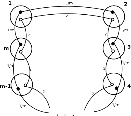
Figure 3: Hard instance $G_{G}$ for GTSP with global structure representation

The clusters are numbered in the figure, and a measure $S$ for evaluating cluster orders is based on this numbering: Let $\pi=(\pi_{1},\ldots,\pi_{m})$ represent the permutation of clusters in the upper layer, then $S(\pi)=|\{i\mid\pi_{(i+1\>\mod\>m)}=(\pi_{i}+1)\;\mod\;m\}|$ indicates the similarity of the permutation with the optimal permutation. A large value of $S(\pi)$ means that many clusters in $\pi$ are in the same order as in the optimal solution. Note that $S(\pi^{*})=m$ for an optimal solution $\pi^{*}$. A solution $\pi$ with $S(\pi)=0$ is locally optimal in the sense that there is no strictly better solution in the neighbourhood induced by the jump operator. The solutions with $S(\pi)=0$ form a plateau where all solutions differ from the optimal solution by $m$ edges.

We first introduce a lemma that will later help us with the proof of the lower bound on the optimization time.

Lemma 9.

Let $\pi$ and $\pi^{\prime}$ be two non-optimal cluster permutations for the instance $G_{G}$. If $S(\pi^{\prime})>S(\pi)$ then $c(\pi^{\prime})>c(\pi)$.

Proof.

In the given instance, all white nodes are connected to each other with a maximum weight of 2. These connections ensure that any permutation of the clusters, can result in a Hamiltonian tour with a cost of at most $2m$. Moreover, all connections between white nodes and black nodes have a weight of $m^{2}$. So the lower level will never choose a combination of white and black nodes because the cost will be more than $m^{2}$ while there is an option of selecting all white nodes with the cost of at most $2m$. On the other hand, for any permutation of clusters other than the Global Optimum, the lower level will not choose any black nodes, because it will not be possible to use all the $1/m$ edges and some $m^{2}$-weighted edges will be used again. Let $a=S(\pi)$ be the number of clusters adjacent to each other correctly from the right side (having the same right-side neighbour as in the Global Optimum) in a solution $\pi$. Then $b=m-a$ is the number of clusters which have a different neighbour on their right. If $\pi$ is not the optimal solution, then the lower level will choose all white nodes. As a result, $a$ edges with weight 2 and $b$ edges with weight 1 will be used in that solution; therefore, the total cost of solution $\pi$ will be $c(\pi)=2a+b=2a+m-a=m+a$. Consider a solution $\pi^{\prime}$ with $a^{\prime}=S(\pi^{\prime})$ and $S(\pi^{\prime})>S(\pi)$. We have $c(\pi^{\prime})=m+a^{\prime}>m+a=c(\pi)$ which completes the proof. ∎

Lemma 9 shows that any non-optimal offspring $\pi^{\prime}$ of a solution $\pi$ is not accepted if it is closer to an optimal solution $\pi^{*}$. This means that the algorithm finds it hard to obtain an optimal solution for $G_{G}$ and leads to an exponential lower bound on the optimization time as shown in the following theorem.

Theorem 10.

Starting with a permutation of clusters chosen uniformly at random, the optimisation time of the tour based (1+1) EA on $G_{G}$ is $\Omega((\frac{m}{2})^{\frac{m}{2}})$ with probability $1-e^{-\Omega(m)}$.

Proof.

Considering $G_{G}$ illustrated in Figure 3, the optimal solution is the tour comprising all edges with weight $\frac{1}{m}$. We consider a typical run of the algorithm consisting of a phase of $T=Cm^{3}$ steps where $C$ is an appropriate constant. For the typical run we show the following:

1. A local optimum $\pi$ with $S(\pi)=0$ is reached with probability $1-e^{-\Omega(m)}$

2. The global optimal solution is not obtained with probability $1-m^{-\Omega(m)}$

Then we state that only a direct jump from the local optimum to the global optimum is possible, and the probability of this event is $O(m^{-m/2})$.

First we show that with high probability $S(\pi_{init})\leq\varepsilon m$ holds for the initial solution $\pi_{init}$, where $\varepsilon$ is a small positive constant.

We count the number of permutations in which at least $\varepsilon m$, $\varepsilon>0$ a small constant, of cluster-neighbourhoods are correct.

We should select $\varepsilon m$ of the clusters to be followed by their specific neighbour, and consider the number of different permutations of $m-\varepsilon m$ clusters:

$$\binom{m}{\varepsilon m}(m-\varepsilon m)!$$ (1)

Some solutions are double-counted in this expression, so the actual number of different solutions with $S(\pi)\geq\varepsilon m$ is less than (1). Therefore, the probability of having more than $\varepsilon m$ clusters followed by their specific cluster, is at most

$$\binom{m}{\varepsilon m}\frac{(m-\varepsilon m)!}{m!}=((\varepsilon m)!)^{-1}=O\left(\left(\frac{\varepsilon m}{2}\right)^{-\frac{\varepsilon m}{2}}\right)$$

Hence, with probability $1-O((\frac{\varepsilon m}{2})^{-\frac{\varepsilon m}{2}})$, $S(\pi_{init})\leq\varepsilon m$ holds and the initial solution has at at most $\varepsilon m$ correctly ordered clusters.

Now we analyze the expected time to reach a solution $\pi$ with $S(\pi)=0$. The probability of a good ordering to change to a bad one is at least

$$\left(\frac{1}{e}\right)\cdot\left(\frac{k}{m}\right)\cdot\left(\frac{m^{2}-m}{m^{2}}\right)^{k}$$

where $k$ is the number of edges which can be changed in each operation. For jump operation $k$ equals $3$. For all $m>2$, it holds that $m<\frac{m^{2}}{2}$, so the probability above is at least

$$\left(\frac{1}{e}\right)\cdot\left(\frac{3}{m}\right)\cdot\left(\frac{1}{2}\right)^{3}=\Omega(m^{-1})$$

Therefore, the expected time for each edge to be replaced with a bad edge is in $O(m)$ and for $m$ edges it is in $O(m^{2})$.

Now we consider a phase of $T=Cm^{3}$ iterations and show that the local optimum is reached with high probability.

Let $C=2C^{\prime}$ and consider a phase of $2C^{\prime}m^{2}$ iterations while assuming that the local optimum is expected to be reached in time $C^{\prime}m^{2}$. Then by means of Markov’s Inequality we have

$$\Pr(T^{\prime}>2C^{\prime}m^{2})\leq\frac{1}{2}.$$

Repeating this $m$ times, the probability of not reaching the local optimum is $2^{-m}$. Therefore, the algorithm reaches the local optimum with probability $1-2^{-m}=1-e^{-\Omega(m)}$ during the phase of $T=Cm^{3}$ steps.

To prove that with high probability, the global optimum is not reached during the considered phase, note first that by Lemma 9, any jump to a solution closer to the optimum other than directly to the Global Optimum will be rejected.

Furthermore, for the initial solution $S(\pi_{init})\leq\varepsilon m$. Therefore, only non-optimal solutions $\pi$ with $S(\pi)\leq\varepsilon m$ are accepted by the algorithm. In order to obtain an optimal solution the algorithm has to produce the optimal solution from a solution $\pi$ with $S(\pi)\leq\varepsilon m$ in a single mutation step. We now upper bound the probability of such a direct jump which changes at least $(1-\varepsilon)m$ clusters to their correct order. Such a move needs at least $\frac{(1-\varepsilon)m}{3}$ operations in the same iteration. Taking into account that these Jump operations may be acceptable in any order, the probability of a direct jump is at most

$$\frac{1}{e\left(\frac{(1-\varepsilon)m}{3}\right)!}.\frac{1}{m^{\frac{(1-\varepsilon)m}{2}}}\cdot\left(\frac{(1-\varepsilon)m}{3}\right)!=m^{-\Omega(m)}.$$ (2)

So in a phase of $O(m^{3})$ iterations the probability of having such a direct jump is by union bound at most $m^{-\Omega(m)+3}=m^{-\Omega(m)}$.

So far we have shown that a local optimum $\pi$ with $S(\pi)=0$ is reached with probability $1-e^{-\Omega(m)}$ within the first $T=Cm^{3}$ iterations.

The probability of obtaining an optimal solution from a solution $\pi$ with $S(\pi)=0$ is at most

$$\frac{1}{e\left(\frac{m}{3}\right)!}\cdot\frac{1}{m^{\frac{m}{2}}}\cdot\left(\frac{m}{3}\right)!=e^{-1}\cdot m^{-\frac{m}{2}}$$

We now consider an additional phase of $(\frac{m}{2})^{\frac{m}{2}}$ steps after having obtained a local optimum. Using the union bound, the probability of reaching the global optimum in this phase is at most

$$\left(\frac{m}{2}\right)^{\frac{m}{2}}\cdot e^{-1}\cdot m^{-\frac{m}{2}}\leq\left(\frac{1}{2}\right)^{\frac{m}{2}}.$$

As a result, the probability of not reaching the optimal solution in these $(\frac{m}{2})^{\frac{m}{2}}$ iterations is $1-2^{-\frac{m}{2}}=1-e^{-\Omega(m)}$. Altogether, the optimization time is at least $(\frac{m}{2})^{\frac{m}{2}}$ with probability $1-e^{-\Omega(m)}$. ∎

4 Discussion of Generalisations

The problems we have examined in this work are bilevel optimisation problems where the upper level problem, namely the leader, and the lower level problem, the follower, shares an objective function. The general bilevel optimisation problem also includes the setting where the leader and the follower have different objectives. Given the decision of the leader, the follower makes a decision according to his objective function which might be conflicting with the objective function of the leader. An example of such a problem is where the leader places toll booths across a road network and the followers try to find the cheapest way from a point A to a point B by finding a path that avoids as many toll booths as possible. Here, the leader can only learn the objective function value of its decision after the follower picks the optimum path. Unlike the GMSTP and GTSP, the objective functions of upper and lower level problems are conflicting in this toll booth problem.

For a given solution visited in the upper level problem, the evaluation cost is, in the worst case, the computational complexity of the lower level problem. If the lower level problem can be solved in polynomial time, then a fixed-parameter bound on the the size of the upper level solution is sufficient for a fixed-parameter tractable problem. For when the upper level solution is bounded by a parameter k of the original problem, any global random search heuristic on the upper level problem will be able to find the optimal upper level solution in no more than $f(k)$ iterations for some function $f(k)$ and will make $f(k)\cdot\operatorname{poly}(n)$ basic operations in total.

In our case, the Global structure representation of GMSTP and GTSP, the size of an upper level solution is bounded above by $m^{2}$ since it is enough to indicate whether any two clusters are connected or not to precisely define a solution. On the other hand the spanned-nodes representation of GMSTP needs a size of $m\log(n)$ to represent which node is selected in each cluster. If the solution size is restricted by a parameter $m$, uniform random search on the bitstring of length $O(f(m))$ will find the optimal solution in $2^{O(f(m))}$ iterations in expectation. With Global structure representation, if we pick our solutions uniformly at random the probability of picking a unique optimal solution is $(1/2)^{m^{2}}$ which will occur in $O(m^{2m})$ time in expectation while uniform random search with the spanned node representation takes $\Omega(n^{m})$ trials in expectation.

Conclusions

Evolutionary bilevel optimization has gained an increasing interest in recent years. With this article we have contributed to the theoretical understanding by considering two classical NP-hard combinatorial optimization problems, namely the generalized minimum spanning tree problem and the generalized traveling salesperson problem. We studied evolutionary algorithms for the mentioned problems in the parameterized setting. Using parameterised computational complexity analysis of evolutionary algorithms for the generalized minimum spanning tree problem, we have examined two representations for the upper layer solutions and their corresponding deterministic algorithms for the lower layer. Our results show that the Global Structure Representation leads to fixed parameter evolutionary algorithms. By presenting hard instances for each of the two approaches, we have pointed out where they run into difficulties. Furthermore, we have shown that the two representations for the generalized minimum spanning tree problem are highly complementary by proving that they are highly efficient on the hard instance of the other algorithm. After having achieved these results for the generalized minimum spanning tree problem, we turned our attending to the generalized traveling salesperson problem. We showed that using the global structure representation leads to fixed parameter evolutionary algorithms with respect to the number of clusters. Furthermore, we pointed out a worst case instance where the optimization time grows exponential with respect to the number of clusters and discussed generalizations of the results.

References

- Auger and Doerr, (2011) Auger, A. and Doerr, B., editors (2011). Theory of Randomized Search Heuristics: Foundations and Recent Developments. World Scientific.
- Corus et al., (2013) Corus, D., Lehre, P. K., and Neumann, F. (2013). The generalized minimum spanning tree problem: a parameterized complexity analysis of bi-level optimisation. In Blum, C. and Alba, E., editors, GECCO, pages 519–526. ACM.
- Deb and Sinha, (2009) Deb, K. and Sinha, A. (2009). Solving bilevel multi-objective optimization problems using evolutionary algorithms. In Ehrgott, M., Fonseca, C. M., Gandibleux, X., Hao, J.-K., and Sevaux, M., editors, EMO, volume 5467 of Lecture Notes in Computer Science, pages 110–124. Springer.
- Deb and Sinha, (2010) Deb, K. and Sinha, A. (2010). An efficient and accurate solution methodology for bilevel multi-objective programming problems using a hybrid evolutionary-local-search algorithm. Evolutionary Computation, 18(3):403–449.
- Downey and Fellows, (1999) Downey, R. G. and Fellows, M. R. (1999). Parameterized Complexity. Springer-Verlag. 530 pp.
- Fischetti et al., (1997) Fischetti, M., Salazar González, J. J., and Toth, P. (1997). A branch-and-cut algorithm for the symmetric generalized traveling salesman problem. Operations Research, 45(3):378–394.
- Hu and Raidl, (2011) Hu, B. and Raidl, G. R. (2011). An evolutionary algorithm with solution archive for the generalized minimum spanning tree problem. In Moreno-Díaz, R., Pichler, F., and Quesada-Arencibia, A., editors, EUROCAST (1), volume 6927 of Lecture Notes in Computer Science, pages 287–294. Springer.
- Hu and Raidl, (2012) Hu, B. and Raidl, G. R. (2012). An evolutionary algorithm with solution archives and bounding extension for the generalized minimum spanning tree problem. In Soule, T. and Moore, J. H., editors, GECCO, pages 393–400. ACM.
- Koh, (2007) Koh, A. (2007). Solving transportation bi-level programs with differential evolution. In IEEE Congress on Evolutionary Computation, pages 2243–2250. IEEE.
- Kratsch et al., (2010) Kratsch, S., Lehre, P. K., Neumann, F., and Oliveto, P. S. (2010). Fixed parameter evolutionary algorithms and maximum leaf spanning trees: A matter of mutation. In Proceedings of the Eleventh Conference on Parallel Problem Solving from Nature, pages 204–213.
- Kratsch and Neumann, (2013) Kratsch, S. and Neumann, F. (2013). Fixed-parameter evolutionary algorithms and the vertex cover problem. Algorithmica, 65(4):754–771.
- Legillon et al., (2012) Legillon, F., Liefooghe, A., and Talbi, E.-G. (2012). Cobra: A cooperative coevolutionary algorithm for bi-level optimization. In IEEE Congress on Evolutionary Computation, pages 1–8. IEEE.
- Motwani and Raghavan, (1995) Motwani, R. and Raghavan, P. (1995). Randomized Algorithms. Cambridge University Press.
- Myung et al., (1995) Myung, Y.-S., ho Lee, C., and wan Tcha, D. (1995). On the generalized minimum spanning tree problem. Networks, 26(4):231–241.
- Neumann and Witt, (2010) Neumann, F. and Witt, C. (2010). Bioinspired Computation in Combinatorial Optimization:Algorithms and Their Computational Complexity. Springer-Verlag New York, Inc., New York, NY, USA, 1st edition.
- Pop, (2004) Pop, P. C. (2004). New models of the generalized minimum spanning tree problem. J. Math. Model. Algorithms, 3(2):153–166.
- (17) Sutton, A. M. and Neumann, F. (2012a). A parameterized runtime analysis of evolutionary algorithms for the euclidean traveling salesperson problem. In Hoffmann, J. and Selman, B., editors, AAAI. AAAI Press. Extended technical report available at http://arxiv.org/abs/1207.0578.
- (18) Sutton, A. M. and Neumann, F. (2012b). A parameterized runtime analysis of simple evolutionary algorithms for makespan scheduling. In Proceedings of the Twelfth Conference on Parallel Problem Solving from Nature (PPSN 2012), pages 52–61. Springer.