DJ-MC: A Reinforcement-Learning Agent for Music Playlist Recommendation

Abstract

In recent years, there has been growing focus on the study of automated recommender systems. Music recommendation systems serve as a prominent domain for such works, both from an academic and a commercial perspective. A fundamental aspect of music perception is that music is experienced in temporal context and in sequence. In this work we present DJ-MC, a novel reinforcement-learning framework for music recommendation that does not recommend songs individually but rather song sequences, or playlists, based on a model of preferences for both songs and song transitions. The model is learned online and is uniquely adapted for each listener. To reduce exploration time, DJ-MC exploits user feedback to initialize a model, which it subsequently updates by reinforcement. We evaluate our framework with human participants using both real song and playlist data. Our results indicate that DJ-MC’s ability to recommend sequences of songs provides a significant improvement over more straightforward approaches, which do not take transitions into account.

1 Introduction

Music is one of the most widespread and prevalent expressions of human culture. It has accompanied the human experience throughout history, and the enjoyment of music is one of the most common human activities. As an activity, music listening sessions commonly span over a sequence of songs, rather than a single song in isolation. Importantly, it is well established that music is experienced in temporal context and in sequence davies1978psychology ; kahnx1997patterns . This phenomenon not only underlies the notion of structure in music (as in the canonical sonata form cook1994guide ), but also implies that the pleasure one derives from a complete song is directly affected by its relative position in a sequence. This notion also underlies the manner in which DJs construct playlists cliff2000hang , and indeed, research on automated playlist construction has aimed to produce generally appealing playlists oliver2006papa ; crampes2007automatic . However, such works have not considered the construction of personalized playlists tailored to individual users’ preferences.

In the field of recommender systems, adomavicius2005toward music has been of particular interest, both academically adomavicius2005toward ; o2005trust and commercially barrington2009smarter . Pandora, Jango, and Last.fm are some examples of popular contemporary commercial applications. To the best of our knowledge, however, research on personalized music recommendations has focused mostly on predicting users’ preferences over individual songs, rather than song sequences.

Overall, there has been little effort to relate learning individual listener preferences with holistic playlist generation. In this paper, we aim to bridge this gap and present DJ-MC, a novel framework for adaptive, personalized music playlist recommendation. In this framework, we formulate the playlist recommendation problem as a sequential decision making task, and borrow tools from the reinforcement learning literature to learn preferences over both songs and song transitions on the fly. Our contributions are as follows. First, we formulate the problem of selecting which sequence of songs to play as a Markov Decision Process, and demonstrate the potential effectiveness of a reinforcement-learning based approach in a new practical domain. Second, we test the hypothesis that sequence does have a significant effect on listener experience through a user study. Third, we show empirically that DJ-MC’s account for song order allows it to outperform recommendations based strictly on individual song preferences, implying such preferences can be learned efficiently with limited user information. In particular, we demonstrate that starting with no knowledge of a new user’s preferences, DJ-MC is able to generate personalized song sequences within a single listening session of just 25–50 songs.

The remainder of this paper is organized as follows. In Section $2$ we discuss our reformulation of playlist generation as a reinforcement learning task. In Section $3$ we describe how the DJ-MC agent models different aspects of the MDP for the purpose of learning. In Section $4$ we present the real-world data sources we used in this paper. In Section $5$ we present the full DJ-MC agent architecture. In Section $6$ we discuss the performance of DJ-MC in simulation, and in Section $7$ we present the results of applying DJ-MC in a user study with human participants. In Section $8$ we discuss related work and put our contributions in a broader context, and finally in Section $9$ we summarize and discuss our results.

2 Reinforcement Learning Framework

We consider the adaptive playlist generation problem formally as an episodic Markov Decision Process (MDP). An episodic MDP is a tuple $(S,A,P,R,T)$ where $S$ is the set of states; $A$ the set of actions, $P:S\times A\times S\rightarrow[0,1]$ is the state transition probability function where $P(s,a,s^{\prime})=r$ denotes the probability of transitioning from state $s$ to state $s^{\prime}$ when taking action $a$. $R:S\times A\rightarrow\mathbb{R}$ is the state-action reward function, where $R(s,a)=r$ means that taking action $a$ from state $s$ will yield reward $r$. $T$ is the set of terminal states, which end the episode.

For the purposes of our specific application, consider a finite set of $n$ musical tracks (songs) $\cal{M}$ $=\{a_{1},a_{2},\ldots,a_{n}\}$ and assume that playlists are of length $k$. Our MDP formulation of the music playlist recommendation task is then as follows.

• To capture the complex dependency of listener experience on the entire sequence of songs heard, a Markov state must include an ordered list of all prior songs in the playlist. Thus, the state space $S$ is the entire ordered sequence of songs played, $S=\{(a_{1},a_{2},\ldots,a_{i})|1\leq i\leq k;\forall j\leq i,a_{j}\in\cal{M}\}$.

  That is, a state $s\in S$ is an ordered tuple of songs ranging in length from 0 when choosing the first song of the playlist to $k$ when the playlist is complete.

• The set of actions $A$ is the selection of the next song to play, $a_{k}\in A$. This means that the action space is exactly the set of songs: $A=\cal{M}$.

• These definitions of $S$ and $A$ induce a deterministic transition function $P$. As such, we can use the shorthand notation $P(s,a)=s^{\prime}$ to indicate that when taking action $a$ in state $s$, the probability of transitioning to $s^{\prime}$ is 1, and to $s^{\prime\prime}\neq s^{\prime}$ is 0. Specifically, $P((a_{1},a_{2},\ldots,a_{i}),a^{*})=(a_{1},a_{2},\ldots,a_{i},a^{*})$.

• $R(s,a)$ is the utility (or pleasure) the current listener derives from hearing song $a$ when in state $s$. Note that this formulation implies that each listener induces a unique reward function. A key challenge addressed in this paper is enabling efficient learning of $R$ for a new listener.

• $T=\{(a_{1},a_{2},\ldots m_{k})\}$: the set of playlists of length $k$.

Solving an MDP typically refers to finding a policy $\pi:S\rightarrow A$ such that from any given state $s$, executing action $\pi(s)$ and then acting optimally (following the optimal policy $\pi^{*}$) thereafter, yields the highest (expected) sum of rewards over the length of the episode. In our case, since $P$ is deterministic, $\pi*$ corresponds to the single sequence of songs that would be most pleasing to the listener. However, we assume that the listener’s reward function $R$ is initially unknown. We consider the fundamental challenge of playlist generation as being efficiently modeling $R$.

In particular, in the reinforcement learning literature, there are two high-level approaches to approximating (learning) $\pi^{*}$: model-free and model-based. Model-free approaches learn the value of taking an action $a$ from state $s$ directly. Typical approaches, such as $Q$-learning and SARSA Sutton1998 are computationally efficient and elegant, but require a lot of experiential data to learn. Model-based approaches alternatively learn the transition and reward functions ($P$ and $R$) so as to be able to simulate arbitrary amounts of experiential data in order to find an approximate solution to the MDP in an approach that can be thought of as planning through forward lookahead search. Compared to model-free methods, most model-based algorithms are significantly more computationally expensive, especially if they re-solve the MDP whenever the model changes. However, in many applications, including playlist recommendation, where data is considerably more scarce than computation, this tradeoff of computational expense for data efficiency is a good one. We therefore adopt a model-based learning approach in this paper (see Sections 3 and 5 for details).

In the MDP defined above, the transition function $P$ is trivially known. Therefore the only unknown element of the model necessary for model-based learning is $R$, the current listener’s utility (enjoyment) function. Indeed modeling $R$ in such a way that generalizes aggressively and accurately across both songs and song transitions is the biggest technical challenge in this work. Consider that even for a moderately sized music corpus of $10^{3}$ songs, and for playlist horizons of $10$ songs, the size of the state space alone would be $10^{30}$. It is impractical for a learning agent to even explore any appreciable size of this state space, let alone learn the listener’s utility for each possible state (indeed our objective is to learn a new user’s preferences and generate a personalized song sequence within a single listening session of 25–50 songs). Therefore to learn efficiently, the agent must internally represent states and actions in such a way that enables generalization of the listener’s preferences.

Section $3$ presents how DJ-MC compactly represents $R$ by 1) generalizing across songs via a factored representation; and 2) separating $R$ into two distinct components, one dependent only on the current song ($a$), and one dependent on the transition from the past history of songs to the current song ($s$ to $a$). Recognizing that DJ-MC’s specific representation of $R$ is just one of many possible options, we also evaluate the extent to which the representational choices made are effective for generalization and learning.

3 Modeling

As motivated in the previous section, learning a listener’s preference function over a large set of songs and sequences requires a compact representation of songs that is still rich enough to capture meaningful differences in how they are perceived by listeners. To this end, we represent each song as a vector of song descriptors.

Specifically DJ-MC uses spectral auditory descriptors that include details about the spectral fingerprint of the song, its rhythmic characteristics, its overall loudness, and their change over time. We find that these descriptors enable a great deal of flexibility (for instance, in capturing similarities between songs from vastly different backgrounds, or the ability to model songs in unknown languages). Nonetheless, our framework is in principle robust to using any sufficiently expressive vector of song descriptors. Section $3.1$ specifies in detail the descriptors used by DJ-MC.

In order to further speed up learning, we make a second key representational choice, namely that the reward function $R$ corresponding to a listener can be factored as the sum of two distinct components: 1) the listener’s preference over songs in isolation, $R_{s}:A\rightarrow\mathbb{R}$ and 2) his preference over transitions from past songs to a new song, $R_{t}:S\times A\rightarrow\mathbb{R}$. That is, $R(s,a)=R_{s}(a)+R_{t}(s,a)$.

Section $3.2$ describes DJ-MC’s reward model in detail. Section $3.3$ then evaluates the extent to which the chosen descriptors are able to differentiate meaningfully between song sequences that are clearly good and clearly bad.

3.1 Modeling Songs

As motivated above, we assume each song can be factored as a vector of scalar descriptors that reflect details about the spectral fingerprint of the song, its rhythmic characteristics, its overall loudness, and their change over time. For the purpose of our experiments, we used the acoustic features in the Million Song Dataset representation bertin2011million to extract $12$ meta-descriptors, out of which $2$ are $12$-dimensional, resulting in a $34$-dimensional song descriptor vector. The complete set of descriptors is summarized in Table $1$.

Descriptors	Descriptor Indices
10th and 90th percentiles of tempo	1,2
average and variance of tempo	3,4
10th and 90th percentiles of loudness	5,6
average and variance of loudness	7,8
pitch dominance	9–20
variance of pitch dominance	21
average timbre weights	22–33
variance in timbre	34

Table 1: Descriptors used for song representation. Tempo data was based on beat durations. Thus the first descriptor is the 10th percentile of beat durations in the song. Loudness was straightforwardly obtained from amplitude. Pitch dominance weights each of the $12$ possible pitch classes based on their presence in the song averaged over time. Timbre weights are the average weights of the $12$ basis functions used by the Echo Nest analysis tool to capture the spectro-temporal landscape of the song.

3.2 Modeling The Listener Reward Function

Despite an abundance of literature on the psychology of human musical perception tan2010psychology , there is no canonical model of the human listening experience. In this work we model listening as being dependent not only on preferences over the descriptors laid out above, but also over feature transitions. This model is fairly consistent with many observed properties of human perception, such as the stochastic dependence on remembering earlier events, and evidence of working memory having greater emphasis on the present davies1978psychology ; berz1995working ; tan2010psychology .

We now proceed to specify the two components of $R$: $R_{s}$ and $R_{t}$.

3.2.1 Listener Reward Function over Songs $R_{s}$

To model $R_{s}$, we use a sparse encoding of the song descriptors to generate a binary feature vector. $R_{s}$ is then a linear function of this feature vector: that is, we assume that each feature contributes independently to the listener’s utility for the song.

Specifically, for each song descriptor, we collect statistics over the entire music database, and quantize the descriptor into 10-percentile bins. Following standard reinforcement learning notation, we denote the feature vector for song $a$ as $\theta_{s}(a)$. It is a vector of size $\#bins\times\#descriptors=10\times 34=340$ consisting of $\#descriptors$ containing 1’s at coordinates that correspond to the bins song $a$ populates, and $0$ otherwise, meaning $\theta_{s}(a)$ behaves as an indicator function (the weight of $\theta_{s}(a)$ will be 34 overall).

For each feature, we assume the listener has a value representing the pleasure they obtains from songs with that feature active. These values are represented as a weight vector $\phi_{s}(u)$. Thus $R_{s}(a)=\phi_{s}(u)\cdot\theta_{s}(a)$. The parameters of $\phi_{s}(u)$ must be learned afresh for each new user.

3.2.2 Listener Reward Function over Transitions $R_{t}$

A main premise of this work is that in addition to the actual songs played, a listener’s enjoyment depends on the sequence in which they are played. To capture this dependence, we assume that

$$E[R_{t}((a_{1},\ldots,a_{t-1}),a_{t})]=\sum\limits_{i=1}^{t-1}\frac{1}{i^{2}}r_{t}(a_{t-i},a_{t})$$

where $r_{t}(a_{i},a_{j})$ represents the listener’s utility for hearing song $a_{j}$ sometime after having heard $a_{i}$. The term $\frac{1}{i^{2}}$ represents the notion that a song that was played $i$ songs in the past has a probability of $\frac{1}{i}$ of affecting the transition reward (i.e. being “remembered”), and when it does, its impact decays by a second factor of $\frac{1}{i}$ (its impact decays over time).

It remains only to specify the song to song transition reward function $R_{t}(a_{i},a_{j})$. Like $R_{s}$, we can describe $R_{t}$ as a linear function of a sparse binary feature vector: $R_{t}(a_{i},a_{j})=\phi_{t}(u)\cdot\theta_{t}(a_{i},a_{j})$ where $\phi_{t}(u)$ is a user-dependent weight vector and $\theta_{t}$ is a binary feature vector.

Were we to consider the transitions between all 340 features of both $a_{i}$ and $a_{j}$, $\theta_{t}$ would need to be of length $340^{2}>100,000$. For the sake of learnability, we limit $\theta_{t}$ and $\phi_{t}$ to only represent transitions between 10-percentile bins of the same song descriptors. That is, there is for each of the 34 song descriptors, there are 100 features, one of which is 1 and 99 of which are 0, indicating which pair of 10-percentile bins were present in songs $a_{i}$ and $a_{j}$. Therefore, overall, $\theta_{t}$ consists of 3,400 binary features, 34 of which are 1’s.

Clearly, this representation is limiting in that it cannot capture the joint dependence of listener utility on transitions between multiple song descriptors. Especially for the pitch class features, these are likely to be relevant. We make this tradeoff in the interest of enabling learning from relatively few examples. Empirical results indicate that this representation captures enough of real peoples’ transition reward to make a difference in song recommendation quality.

Like $\phi_{s}(u)$, the parameters of $\phi_{t}(u)$ must be learned afresh for each new user. Thus all in all, there are 3740 weight parameters to learn for each listener.

With even that many parameters, it is infeasible to experience songs and transitions with all of them active in just 25 songs. However DJ-MC is able to leverage knowledge of even a few transition examples to plan a future sequence of songs that is biased in favor of the positive ones and against the negative ones.

3.3 Expressiveness of the Listener Model

This representation of the listener’s utility function as a 3740-dimensional sparse binary feature vector is just one of many possible representations. A necessary property of a useful representation is that its features are able to differentiate between commonly perceived “good” vs. “bad” sequences, and the DJ-MC agent internally relies on this property when modeling the listener reward function. To evaluate whether our features are expressive enough to allow this differentiation, we examine the transition profile for two types of transitions, “poor” vs. “fair”, both derived from the same population of songs. We generate “fair” transitions by sampling pairs of songs that appeared in an actual sequence. We generate “poor” transitions by interleaving songs so that each one is distinctly different in character (for instance, a fast, loud track followed by a soft piece). The difference between the two profiles can be seen in Figure 1. More definitive evidence in favor of the adequacy of our representation is provided by the successful empirical application of our framework, discussed in Section $7$.

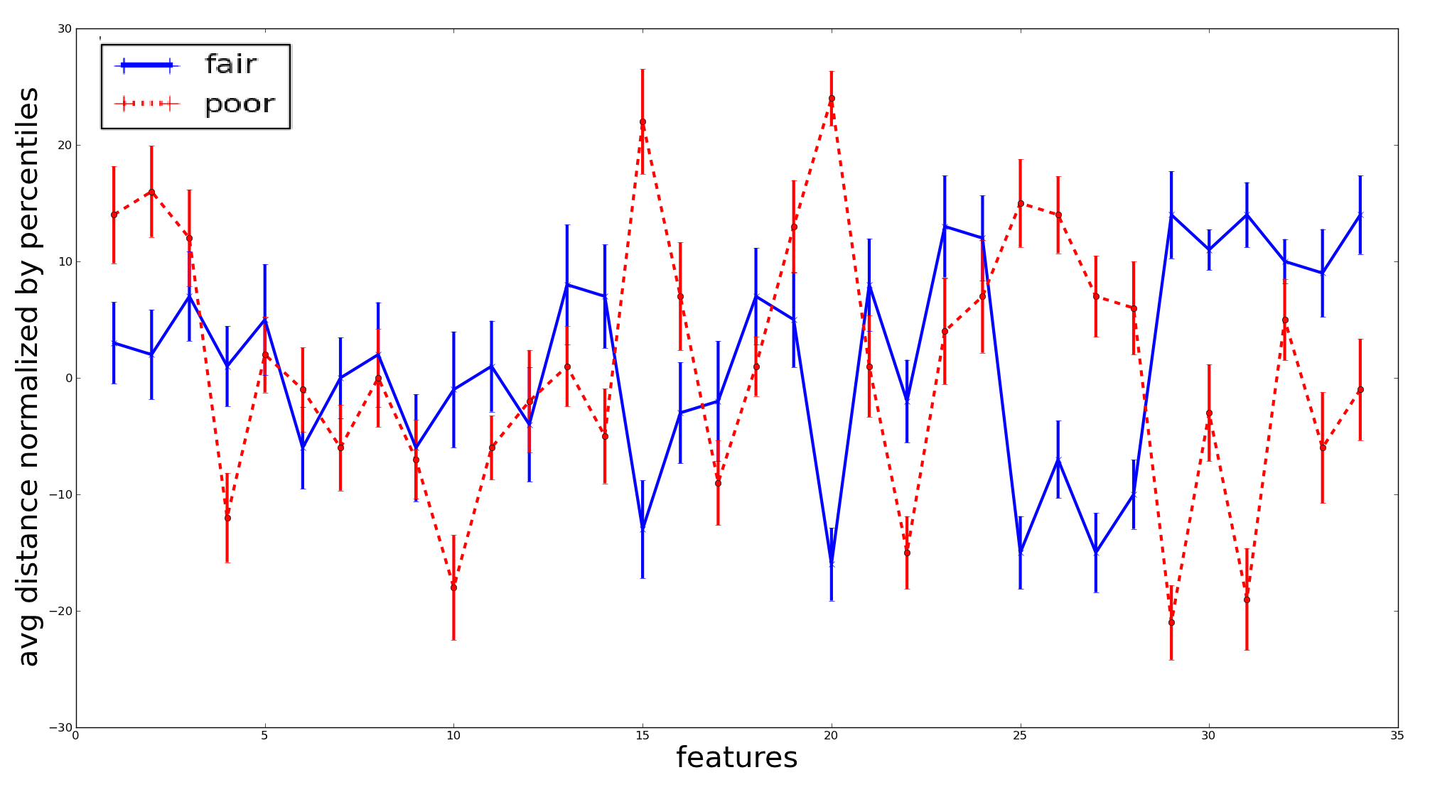
Figure 1: Example of fair vs. poor transition profiles, based on the same set of $20$ songs. The plot shows the average transition delta for each feature. Both the fair transitions and the poor ones are constructed from the same core set of $20$ songs taken from $5$ different albums. In the case of fair transitions, we maintain the original order. In the case of poor transitions, the albums are randomly interleaved. The results indicate that qualitatively different sequences are indeed distinguishable in our feature model. In this specific example, $19$ of the $34$ features are discriminative (confidence intervals do not overlap). We expect different features to be discriminative for different transition profiles.

4 Data

A significant component of this work involves extracting real-world data for both songs and playlists to rigorously test our approach. In this section we discuss the different data sources we used to model both songs and playlists. For songs, we relied on the Million Song Dataset bertin2011million , a freely-available collection of audio features and metadata for a million contemporary popular music tracks. The dataset covers $44,745$ different artists and $10^{6}$ different tracks. All the features described in Table 1 are derived from this representation. An example of the audio input for a single track is provided in Figure 2. It should be noted that our agent architecture (described in detail in Section $5$) is agnostic to the choice of a specific song corpus, and we could have easily used a different song archive.

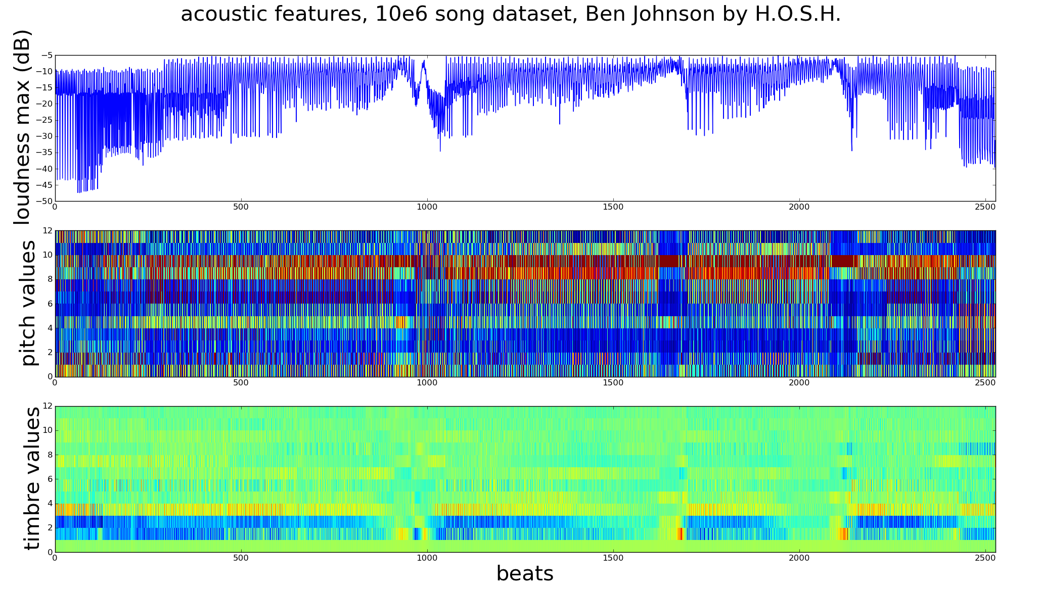
Figure 2: Example of loudness, pitch and timbre data for an example track over time (time units are in beats). Loudness is in dB, pitch measurements are represented as a vector of $12$ values between $0$ and $1$ representing dominance per pitch class. Timbre is approximated as the decomposition of the spectro-temporal surface of the song according to 12 pre-computed basis functions.

To initially test our approach in simulation (a process described in detail in Section $6$), we also needed real playlists to extract song transition data from. A good source of playlists needs to be sufficiently rich and diverse, but also reflect real playlists “in the wild”. In this paper, we used two separate sources. The first, the Yes.com archive, is corpus collected by Chen et al. chen2012playlist . These playlists and related tag data were respectively crawled from Yes.com and Last.fm. Chen et al. harvested data between December 2010 and May 2011, yielding 75,262 songs and 2,840,553 transitions. The second source is the Art of the Mix Archive, collected by Berenzweig et al berenzweig2004large . Berenzweig et al. gathered  29,000 playlists from The Art of the Mix (www.artofthemix.org), a repository and community center for playlist hobbyists. These playlists were (ostensibly) generated by real individual users, rather than a commercial radio DJ or a recommendation system, making this corpus particularly appealing for listener modeling.

5 DJ-MC

In this section we introduce DJ-MC, a novel reinforcement learning approach to a playlist-oriented, personalized music recommendation system. The DJ-MC agent architecture contains two major components: learning of the listener parameters ($\phi_{s}$ and $\phi_{t}$) and planning a sequence of songs. The learning part is in itself divided into two parts - initialization and learning on the fly. Initialization is critical if we wish to engage listeners quickly without losing their interest before the agent has converged on a good enough model. Learning on the fly enables the system to continually improve until it converges on a reliable model for that listening session. In simulation, we assume the user is able to specify an initial list of songs that they like (this is similar to most initialization practices used by commercial music recommendation systems). However, in Section $7$ we show this step can be replaced with random exploration, while still reaching compelling results at the exploitation stage.

The planning step enables the selection of the next appropriate song to play. As pointed out in Section $2$, given the sheer scope of the learning problem, even after various abstraction steps, solving the MDP exactly is intractable. For this reason we must approximate the solution. From a practical perspective, from any given state, the objective is to find a song that is “good enough” to play next. For this purpose we utilize Monte Carlo Tree Search.

In Sections $5.1$ and $5.2$ we describe the initialization steps taken by DJ-MC. In Section $5.3$ we describe the core of the learning algorithm, which learns on the fly. in Section $5.4$ we describe the planning step. The full agent pseudocode is provided in Algorithm 5.

5.1 Learning Initial Song Preferences

To initialize the listener’s song model, DJ-MC polls the listener for his $k_{s}$ favorite songs in the database and passes them as input to Algorithm 1. As a form of smoothing (or of maintaining a uniform prior), each element of $\phi_{s}(u)$ is initialized to $1/(k_{s}+\#bins)$, where $\#bins$ is the granularity of discretization of each song descriptor – in our case 10 (line 2). Then for each favorite song $a$, $\phi_{s}(u)$ is incremented by $1/(k+\#bins)\cdot\theta_{s}(a)$ (line 5). At the end of this process, the weights in $\phi_{s}(u)$ corresponding to each song descriptor sum to 1.

Algorithm 1 Initialize Song Preferences $R_{s}$

1:  Input: Song corpus, $\cal{M}$ Number of preferred songs to be provided by listener, $k_{s}$

2:  initialize all coordinates of $\phi_{s}$ to $1/(k_{s}+\#bins)$

3:  preferredSet = $\{a_{1},\ldots,a_{k_{s}}\}$ (chosen by the listener)

4:  for $i=1$ to $k_{s}$ do

5:     $\phi_{s}=\phi_{s}+\frac{1}{(k_{s}+1)}\cdot\theta_{s}(a_{i})$

6:  end for

5.2 Learning Initial Transition Preferences

In the second stage, the listener is queried for preferences regarding transitions, following the procedure in Algorithm 2. As in the case of initializing song preferences, the predicted value of a transition from bin $i$ to bin $j$ for each feature is initialized to $1/(k_{t}+\#bins)$ where $k_{t}$ is the number of transitions queried and $\#bins$ is the number of feature transition bins – in our case 100 (line 2).

We wouldn’t want to query transitions for too small a subset of preferred songs, because that won’t necessarily reveal enough about the preferred transitions. For this reason we explore the preferences of the listener in a targeted fashion, by presenting them with different possible transitions that encapsulate the variety in the dataset, and directly asking which of a possible set of options the listener would prefer. On the other hand, we would also like to exclude regions in the search space where expected song rewards are low.

To accomplish both ends, DJ-MC first chooses a $50$-% subset of the songs $\cal{M}^{*}$ of the song corpus $\cal{M}$ which, based on its song rewards model, obtains the highest song reward $R_{s}$ (line 3). Then, DJ-MC queries transition preferences over this upper median of songs by eliciting user feedback. It does so by applying the $\delta$-medoids algorithm, a novel method for representative selection (line 5) repsel . This algorithm returns a compact but close-fitting subset of representatives such that no sample in the dataset is more than a parameter $\delta$ away from a representative, thus providing a diverse sample of the upper median of songs. $\delta$ is initialized to be the $10$-th percentile of the distance histogram between all pairs of songs in the database (line 4). We denote the representative subset $\cal{C}$. To model transitions, DJ-MC chooses songs from $\cal{C}$, and queries the listener which song $a_{i}\in\cal{C}$ they would like to listen to next (line 8). For modeling purposes, we assume the listener chooses the next song he would prefer by simulating the listening experience, including the non-deterministic history-dependent transition reward, and choosing the one with the maximal total reward. DJ-MC then proceeds to update the characteristics of this transition, by increasing the weight of transition features by $1/(k+\#bins)$ (line 9) , similarly to how it updated the model for song preferences (so again, the weights of each individual descriptor sum up to $1$). The full details of the algorithm are described in Algorithm 2.

Algorithm 2 Initialize Transition Preferences $R_{t}$

1:  Input: Song corpus $\cal{M}$ Number of transitions to poll the listener, $k_{t}$

2:  initialize all coordinates of $\phi_{t}$ to $1/(k_{t}+\#bins)$

3:  Select upper median of $\cal{M}$, $\cal{M}^{*}$, based on $R_{s}$

4:  $\delta=$ 10th percentile of all pairwise distances between songs in $\cal{M}$

5:  representative set $\cal{C}=\delta$ -medoids $(\cal{M}^{*})$

6:  $song_{0}=$ choose a song randomly from $\cal{C}$

7:  for $i=1$ to $k_{t}$ do

8:     $song_{i}\leftarrow$ chosen by the listener from $\cal{C}$

9:     $\phi_{t}=\phi_{t}+\frac{1}{(k_{t}+1)}\cdot\theta_{t}(song_{i-1},song_{i})$

10:  end for

5.3 Learning on the fly

After initialization, DJ-MC begins playing songs for the listener, requesting feedback, and updating $\phi_{s}$ and $\phi_{t}$ accordingly. For ease of use DJ-MC does not require separate ratings for songs and transitions. Rather, it can assign credit to each component individually from a single unified reward signal. It does so by computing the relative contributions of the song and transition rewards to the total reward as predicted by its model. This update procedure is presented in Algorithm 3.

Specifically, let $r$ be the reward the user assigns after hearing song $a$ in state $s$, and $\bar{r}$ be the average rewards assigned by this listener so far (line 4). We define $r_{incr}=log(\frac{r}{\bar{r}})$ (line 5). This factor determines both direction and magnitude for the update (negative if $r<\bar{r}$, positive otherwise, and greater the farther $r$ is from average). Let $R_{s}(a_{i})$ and $R_{t}(a_{i-1},a_{i})$ be the expected song and transition rewards yielded by our model, respectively. DJ-MC uses the proportions of these values to set weights for credit assignment (this is essentially a maximum likelihood estimate). Concretely, we define the update weights for the song and transition to be

$w_{s}=\frac{R_{s}(a_{i})}{R_{s}(a_{i})+R_{t}(a_{i-1},a_{i})}$ and

$w_{t}=\frac{R_{t}(a_{i-1},a_{i})}{R_{s}(a_{i})+R_{t}(a_{i-1},a_{i})}$ respectively (lines 6-7).

Finally, the agent uses the credit assignment values determined at the previous step to partition the given reward between song and transition weights, and update their values (lines 8-9). Following this step, DJ-MC normalizes both the song and transition reward models so that the weights for each feature sum up to $1$ (line 10). This update procedure as a whole can be perceived as a temporal-difference update with an attenuating learning rate, which balances how much the model “trusts” the previous history of observations compared to the newly obtained signal. It also guarantees convergence over time.

Algorithm 3 Model Update

1:  Input: Song corpus, $\cal{M}$ Planned playlist duration, $K$

2:  for  $i\in\{1,\ldots,K\}$ do

3:     Use Algorithm 4 to select song $a_{i}$, obtaining reward $r_{i}$

4:     let $\bar{r}=average(\{r_{1},\ldots,r_{i-1}\})$

5:     $r_{incr}$ = $log(r_{i}/\bar{r})$ weight update:

6:     $w_{s}=\frac{R_{s}(a_{i})}{R_{s}(a_{i})+R_{t}(a_{i-1},a_{i})}$

7:     $w_{t}=\frac{R_{t}(a_{i-1},a_{i})}{R_{s}(a_{i})+R_{t}(a_{i-1},a_{i})}$

8:     $\phi_{s}=\frac{i}{i+1}\cdot\phi_{s}+\frac{1}{i+1}\cdot\theta_{s}\cdot w_{s}\cdot r_{incr}$

9:     $\phi_{t}=\frac{i}{i+1}\cdot\phi_{t}+\frac{1}{i+1}\cdot\theta_{t}\cdot w_{t}\cdot r_{incr}$

10:     Per $d\in\mbox{descriptors}$, normalize $\phi_{s}^{d},\phi_{t}^{d}$ (where $\phi_{x}^{d}$ denotes coordinates in $\phi_{x}$ corresponding to 10-percentile bins of descriptor $d$)

11:  end for

5.4 Planning

Equipped with the listener’s learned song and transition utility functions $R_{s}$ and $R_{t}$, which determine the MDP reward function $R(s,a)=R_{s}(a)+R_{t}(s,a)$, DJ-MC employs a tree-search heuristic for planning, similar to that used in AAMAS13-urieli . As in the case of initializing the transition weights (Algorithm 2), DJ-MC chooses a subset of $50$-percent of the songs in the database, which, based on $R_{s}$, obtain the highest song reward (line 2). At each point, it simulates a trajectory of future songs selected at random from this “high-yield” subset (lines 7-11). The DJ-MC architecture then uses $R_{s}$ and $R_{t}$ to calculate the expected payoff of the song trajectory (line 12). It repeats this process as many times as possible, finding the randomly generated trajectory which yields the highest expected payoff (lines 13-16). DJ-MC then selects the first song of this trajectory to be the next song played (line 19). It uses just the first song and not the whole sequence because as modeling noise accumulates, its estimates become farther off. Furthermore, as we discussed in Subsection $5.3$, DJ-MC actively adjusts $\phi_{s}$ and $\phi_{t}$ online based on user feedback using Algorithm 3. As a result, replanning at every step is advisable.

If the song space is too large or the search time is limited, it may be infeasible to sample trajectories starting with all possible songs. To mitigate this problem, DJ-MC exploits the structure of the song space by clustering songs according to song types (line 9). It then plans over abstract song types rather than concrete songs, thus drastically reducing search complexity. Once finding a promising trajectory, DJ-MC selects a concrete representative from the first song type in the trajectory to play (line 18).

Algorithm 4 Plan via Tree Search

1:  Input: Song corpus $\cal{M}$, planning horizon $q$

2:  Select upper median of $\cal{M}$, $\cal{M}^{*}$, based on $R_{s}$

3:  BestTrajectory $=null$

4:  HighestExpectedPayoff $=-\infty$

5:  while computational power not exhausted do

6:     $trajectory=[]$

7:     for $1..\ldots q$ do

8:        $song\leftarrow$ selected randomly from $\cal{M}^{*}$ (avoiding repetitions)

9:        optional: $song\_type\leftarrow$ selected randomly from $song\_types(\cal{M}^{*})$ (avoiding repetitions, $song\_types(\cdot)$ reduces the set to clusters)

10:        add $song$ to $trajectory$

11:     end for

12:     $\mbox{expectedPayoffForTrajectory}=R_{s}(song_{1})+\sum\limits_{i=2}^{q}(R_{t}((song_{1},\ldots,song_{i-1}),song_{i})+R_{s}(song_{i}))$

13:     if $\mbox{expectedPayoffForTrajectory}>\mbox{HighestExpectedPayoff}$ then

14:        $\mbox{HighestExpectedPayoff}=\mbox{expectedPayoffForTrajectory}$

15:        BestTrajectory $=$ trajectory

16:     end if

17:  end while

18:  optional: if planning over song types, replace BestTrajectory$[0]$ with concrete song.

19:  return BestTrajectory$[0]$

Combining initialization, learning on the fly, and planning, the full DJ-MC agent architecture is presented in Algorithm 5.

Algorithm 5 Full DJ-MC Architecture

1:  Input: $\cal{M}$ - song corpus, $K$ - planned playlist duration, $k_{s}$ - number of steps for song preference initialization, $k_{t}$ - the number of steps for transition preference initialization Initialization:

2:  Call Algorithm 1 with corpus $\cal{M}$ and parameter $k_{s}$ to initialize song weights $\phi_{s}$.

3:  Call Algorithm 2 with corpus $\cal{M}$ and parameter $k_{t}$ to initialize transition weights $\phi_{t}$. Planning and Model Update:

4:  Run Algorithm 3 with corpus $\cal{M}$ and parameter $K$ (Algorithm 3 iteratively selects the next song to play by calling algorithm 4, and then updates $R_{s}$ and $R_{t}$. This is repeated for $K$ steps.)

6 Evaluation in Simulation

Due to the time and difficulty of human testing, especially in listening sessions lasting hours, it is important to first validate DJ-MC in simulation. To this end, we tested DJ-MC on a large set of listener models built using real playlists made by individuals and included in The Art of the Mix archive. For each experiment, we sample a $1000$-song corpus from the Million Song Dataset.

One of the issues in analyzing the performance of DJ-MC was the nonexistence of suitable competing approaches to compare against. Possible alternatives are either commercial and proprietary, meaning their mechanics are unknown, or they do not fit the paradigm of online interaction with an unknown individual user. Still, we would like our evaluation to give convincing evidence that DJ-MC is capable of learning not only song preferences but also transition preferences to a reasonable degree, and that by taking transition into account DJ-MC is able to provide listeners with a significantly more enjoyable experience (see Section $8$ for related work).

In order to measure the improvement offered by our agent, we compare DJ-MC against two alternative baselines: an agent that chooses songs randomly, and a greedy agent that always plays the song with the highest song reward, as determined by Algorithm 1. As discussed in the introduction, we expect that the greedy agent will do quite well since song reward is the primary factor for listeners. However we find that by learning preferences over transitions, DJ-MC yields a significant improvement over the greedy approach.

To represent different listener types, we generate $10$ different playlist clusters by using $k$-means clustering on the playlists (represented as artist frequency vectors). We generate $1000$ different listeners by first sampling a random cluster, second sampling $70\%$ of the song transition pairs in that cluster, and third inputting this data to Algorithms 1 and 2 to train the listener’s song and transition weights. For the experiments reported here we used a playlist length of 30 songs, a planning horizon of 10 songs ahead, a computational budget of 100 random trajectories for planning, a query size of 10 songs for song reward modeling and 10 songs for transition rewards. As shown in Figure 3, DJ-MC performs significantly better than the baselines, most noticeably in the beginning of the session.

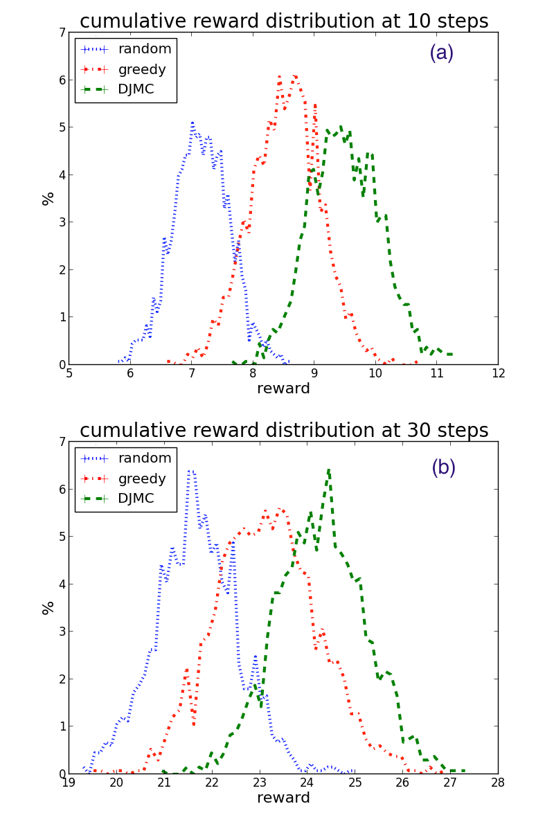
Figure 3: Cumulative reward histograms for playlists of length $10$ (a) and $30$ (b), with listeners based on real playlist data. The DJ-MC agent outperforms both random and greedy agents, particularly for the first $10$ songs. Results are highly significant (p-value $<<0.01$).

7 Evaluation on Human Listeners

While using simulated listeners allows for extensive analysis, ultimately the true measure of DJ-MC is whether it succeeds when applied on real listeners. To test whether this is the case, we ran two rounds of lab experiments with 47 human participants. The participants pool was comprised of graduate students at the McCombs School of Business at the University of Texas at Austin.

7.1 Experimental Setup

Each participant interacted with a playlist generator. As a song corpus we used songs with corresponding Million Song Dataset entries that also appeared in Rolling Stone Magazine’s list of 500 greatest albums of all time. To keep the duration of the experiment reasonable, each song played for 60 seconds before transitioning (with a cross-fade) to the next song. After each song the participants were asked, via a graphic user interface, to specify whether they liked or disliked the played song, as well as the transition to it. This provided us with separate (albeit not independent) signals for song quality and song transition quality to test how well DJ-MC actually did. Since asking users for their selection of $10$ songs was impractical in this setting, in order to seed the learning the agent explored randomly for 25 songs, and then began exploiting the learned model (while continuing to learn) for 25 songs. The participants were divided into 2 groups - 24 interacted with the greedy baseline, whereas 23 interacted with DJ-MC. Though we expect the greedy agent to perform well based on song preferences only, we test whether DJ-MC’s attention to transition preferences improves performance.

7.2 Results

Since our sample of human participants is not large, and given the extremely noisy nature of the input signals, and the complexity of the learning problem, it should come as no surprise that a straightforward analysis of the results can be difficult and inconclusive. To overcome this issue, we take advantage of bootstrap resampling, which is a highly common tool in the statistics literature to estimate underlying distributions using small samples and perform significance tests.

At each stage we treat a “like” signal for either the transition or the song as $+1$ reward value vs. $0$ for a “dislike”. We continue to reconstruct an approximate distribution of the aggregate reward for each condition by sampling subsets of 8 participants with repetition for $N=250000$ times and estimating the average reward value for the subset. Figures 4a and 4c compare the reward distributions for the greedy and DJ-MC agents from song reward and transition reward respectively, during the first 25 episodes. Since both act identically (randomly) during those episodes, the distributions are very close (and indeed testing the hypothesis that the two distributions have means more than $0.25$ apart by offsetting the distributions and running an appropriate t-test does not show significance).

During the exploitation stage (episodes 26-50), the agents behave differently. With regards to song reward, we see that both algorithms are again comparable (and better in expectation than in the exploration stage, implying some knowledge of preference has been learned), as seen in Figure 4b. In Figure 4d, however, we see that DJ-MC significantly outperforms the greedy algorithm in terms of transition reward, as expected, since the greedy algorithm does not learn transition preferences. The results are statistically significant using an unpaired t-test ($p<<0.01$), and are also significant when testing to see if the difference is greater than $0.25$.

Interestingly, the average transition reward is higher for the greedy algorithm at the exploitation stage (apparent by higher average reward comparing Figures 4a and 4b). From this result we can deduce that either people are more likely to enjoy a transition if they enjoy the song, or that focusing on given tastes immediately reduces the “risk” of poor transitions by limiting the song space. All in all, these findings, made with the interaction of human listeners, corroborate our findings based on simulation, that reasoning about transition preferences gives DJ-MC a small but significant boost in performance compared to only reasoning about song preferences.

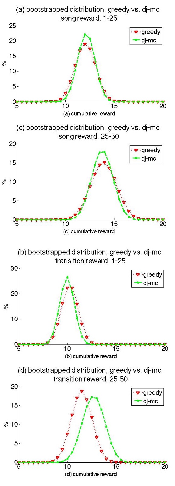
Figure 4: (a) Histogram of cumulative song rewards for the first 25 songs (b) Histogram of cumulative song rewards for the songs 25-50. (c) Histogram of cumulative transition rewards for the first 25 songs. (d) Histogram of cumulative transition rewards for the songs 25-50. Histograms computed via bootstrap resampling the original data 250,000 times.

8 Related Work

Though not much work has attempted to model playlists directly, there has been substantial research on modeling similarity between artists and between songs. Platt et al. platt2003fast use semantic tags to learn a Gaussian process kernel function between pairs of songs. Weston et al. weston2011multi learn an embedding in a shared space of social tags, acoustic features and artist entities by optimizing an evaluation metric for various music retrieval tasks. Aizenberg et al. aizenberg2012build model radio stations as probability distributions of items to be played, embedded in an inner-product space, using real playlist histories for training.

In the academic literature, several recent papers have tried to tackle the issue of playlist prediction. Maillet et al.maillet2009steerable approach the playlist prediction problem from a supervised binary classification perspective, with pairs of songs in sequence as positive examples and random pairs as negative ones. Mcfee and Lanckriet mcfee2011natural consider playlists as a natural language induced over songs, training a bigram model for transitions and observing playlists as Markov chains. Chen et al.chen2012playlist take on a similar Markov approach, treating playlists as Markov chains in some latent space, and learn a metric representation (or multiple representations) for each song in that space, without relying on audio data. In somewhat related work, Zheleva et al.zheleva2010statistical adapt a Latent Dirichlet Allocation model to capture music taste from listening activities across users, and identify both the groups of songs associated with the specific taste and the groups of listeners who share the same taste. In a more recent related work, Natarajan et al. natarajan2013app generalize this approach to the problem of collaborative filtering for interactional context. Users are clustered based on a one-step transition probability between items, and then transition information is generalized across clusters. Another recent work by Wang et al. wang2013exploration also borrows from the reinforcement learning literature, and considers the problem of song recommendations as a bandit problem. Applying this approach, the authors attempt to balance the tradeoff between exploration and exploitation in personalized song recommendation.

The key difference between these approaches and our methodology is that to the best of our knowledge, no one has attempted to model entire playlists adaptively, while interacting with a human listener individually and learning his preferences over both individual songs and song transitions online. By explicitly modeling transitions and exploiting user reinforcement, our framework is able to learn preference models for playlists on the fly without any prior knowledge.

9 Summary and Discussion

In this work we present DJ-MC, a full DJ framework, meant to learn the preferences of an individual listener online, and generate suitable playlists adaptively. In the experimental sections we show that our approach offers significant improvement over a more standard approach, which only considers song rewards. DJ-MC, which focuses on the audio properties of songs, has the advantage of being able to generate pleasing playlists that are unexpected with respect to traditional classifications based on genre, period, etc. In future work, it would be of interest to combine intrinsic sonic features with varied sources of metadata (e.g. genre, period, tags, social data, artist co-occurrence rates, etc). It would also be of interest to test our framework on specific types of listeners and music corpora. This work shows promise for both creating better music recommendation systems, and demonstrating the effectiveness of a reinforcement-learning based approach in a new practical domain.

Acknowledgements

This work has taken place in the Learning Agents Research Group (LARG) at the Artificial Intelligence Laboratory, The University of Texas at Austin. LARG research is supported in part by grants from the National Science Foundation (CNS-1330072, CNS-1305287), ONR (21C184-01), AFOSR (FA8750-14-1-0070, FA9550-14-1-0087), and Yujin Robot.

References

- [1] G. Adomavicius and A. Tuzhilin. Toward the next generation of recommender systems: A survey of the state-of-the-art and possible extensions. Knowledge and Data Engineering, IEEE Transactions on, 17(6):734–749, 2005.
- [2] N. Aizenberg, Y. Koren, and O. Somekh. Build your own music recommender by modeling internet radio streams. In Proceedings of the 21st international conference on World Wide Web, pages 1–10. ACM, 2012.
- [3] L. Barrington, R. Oda, and G. Lanckriet. Smarter than genius? human evaluation of music recommender systems. In International Symposium on Music Information Retrieval, 2009.
- [4] A. Berenzweig, B. Logan, D. P. Ellis, and B. Whitman. A large-scale evaluation of acoustic and subjective music-similarity measures. Computer Music Journal, 28(2):63–76, 2004.
- [5] T. Bertin-Mahieux, D. P. Ellis, B. Whitman, and P. Lamere. The million song dataset. In ISMIR 2011: Proceedings of the 12th International Society for Music Information Retrieval Conference, October 24-28, 2011, Miami, Florida, pages 591–596. University of Miami, 2011.
- [6] W. L. Berz. Working memory in music: A theoretical model. Music Perception, pages 353–364, 1995.
- [7] S. Chen, J. L. Moore, D. Turnbull, and T. Joachims. Playlist prediction via metric embedding. In Proceedings of the 18th ACM SIGKDD international conference on Knowledge discovery and data mining, pages 714–722. ACM, 2012.
- [8] D. Cliff. Hang the dj: Automatic sequencing and seamless mixing of dance-music tracks. HP LABORATORIES TECHNICAL REPORT HPL, (104), 2000.
- [9] N. Cook. A guide to musical analysis. Oxford University Press, 1994.
- [10] M. Crampes, J. Villerd, A. Emery, and S. Ranwez. Automatic playlist composition in a dynamic music landscape. In Proceedings of the 2007 international workshop on Semantically aware document processing and indexing, pages 15–20. ACM, 2007.
- [11] J. B. Davies and J. B. Davies. The psychology of music. Hutchinson London, 1978.
- [12] B. Kahnx, R. Ratner, and D. Kahneman. Patterns of hedonic consumption over time. Marketing Letters, 8(1):85–96, 1997.
- [13] E. Liebman, B. Chor, and P. Stone. Representative selection in non metric datasets. eprint arXiv:1502.07428, 2015.
- [14] J. MacQueen et al. Some methods for classification and analysis of multivariate observations. In Proceedings of the fifth Berkeley symposium on mathematical statistics and probability, volume 1, pages 281–297. California, USA, 1967.
- [15] F. Maillet, D. Eck, G. Desjardins, P. Lamere, et al. Steerable playlist generation by learning song similarity from radio station playlists. In ISMIR, pages 345–350, 2009.
- [16] B. McFee and G. R. Lanckriet. The natural language of playlists. In ISMIR, pages 537–542, 2011.
- [17] N. Natarajan, D. Shin, and I. S. Dhillon. Which app will you use next?: collaborative filtering with interactional context. In Proceedings of the 7th ACM conference on Recommender systems, pages 201–208. ACM, 2013.
- [18] J. O’Donovan and B. Smyth. Trust in recommender systems. In Proceedings of the 10th international conference on Intelligent user interfaces, pages 167–174. ACM, 2005.
- [19] N. Oliver and L. Kreger-Stickles. Papa: Physiology and purpose-aware automatic playlist generation. In Proc. 7th Int. Conf. Music Inf. Retrieval, pages 250–253, 2006.
- [20] J. C. Platt. Fast embedding of sparse similarity graphs. In Advances in Neural Information Processing Systems, page None, 2003.
- [21] R. S. Sutton and A. G. Barto. Introduction to Reinforcement Learning. MIT Press, Cambridge, MA, USA, 1st edition, 1998.
- [22] S.-L. Tan, P. Pfordresher, and R. Harré. Psychology of music: From sound to significance. Psychology Press, 2010.
- [23] D. Urieli and P. Stone. A learning agent for heat-pump thermostat control. In Proceedings of the 12th International Conference on Autonomous Agents and Multiagent Systems (AAMAS), May 2013.
- [24] X. Wang, Y. Wang, D. Hsu, and Y. Wang. Exploration in interactive personalized music recommendation: A reinforcement learning approach. arXiv preprint arXiv:1311.6355, 2013.
- [25] J. Weston, S. Bengio, and P. Hamel. Multi-tasking with joint semantic spaces for large-scale music annotation and retrieval. Journal of New Music Research, 40(4):337–348, 2011.
- [26] E. Zheleva, J. Guiver, E. Mendes Rodrigues, and N. Milić-Frayling. Statistical models of music-listening sessions in social media. In Proceedings of the 19th international conference on World wide web, pages 1019–1028. ACM, 2010.